跳到论文正文
W Papers独立论文阅读器 arXiv:2002.10940 论文正文 计算阅读时间 · 0%
引用这篇论文根据当前论文元数据生成,正式投稿前建议核对。


License: arXiv.org perpetual non-exclusive license
arXiv:2002.10940v5 [cs.LG] 27 Sep 2021

Stochastic-Sign SGD for Federated Learning with Theoretical Guarantees

Richeng Jin,    Yufan Huang,    Xiaofan He,    Huaiyu Dai,    Tianfu Wu Thanks: North Carolina State University, Email: rjin2@ncsu.edu. Thanks: North Carolina State University, Email: yhuang20@ncsu.edu. Thanks: Wuhan University, Email: xiaofanhe@whu.edu.cn. Thanks: Corresponding author; North Carolina State University, Email: hdai@ncsu.edu. Thanks: North Carolina State University, Email: tianfu_wu@ncsu.edu.
Abstract

Federated learning (FL) has emerged as a prominent distributed learning paradigm. FL entails some pressing needs for developing novel parameter estimation approaches with theoretical guarantees of convergence, which are also communication efficient, differentially private and Byzantine resilient in the heterogeneous data distribution settings. Quantization-based SGD solvers have been widely adopted in FL and the recently proposed SIGNSGD with majority vote shows a promising direction. However, no existing methods enjoy all the aforementioned properties. In this paper, we propose an intuitively-simple yet theoretically-sound method based on SIGNSGD to bridge the gap. We present Stochastic-Sign SGD which utilizes novel stochastic-sign based gradient compressors enabling the aforementioned properties in a unified framework. We also present an error-feedback variant of the proposed Stochastic-Sign SGD which further improves the learning performance in FL. We test the proposed method with extensive experiments using deep neural networks on the MNIST dataset and the CIFAR-10 dataset. The experimental results corroborate the effectiveness of the proposed method.

1 Introduction

Recently, Federated Learning (FL) has become a prominent distributed learning paradigm since it allows training on a large amount of decentralized data residing on devices like mobile phones [1]. However, FL imposes several critical challenges. First of all, the communication capability of the mobile devices can be a significant bottleneck. Furthermore, the training data on a given worker is typically based on its usage of the mobile devices, which results in heterogeneous data distribution. In addition, the local data usually contains some sensitive information of a particular mobile device user. Therefore, there is an pressing need to develop a privacy-preserving distributed learning algorithm. Finally, similar to many distributed learning methods, FL may suffer from malicious participants. As is shown in [2], even a single Byzantine worker, which may transmit arbitrary information, can severely disrupt the convergence of distributed gradient descent algorithms. However, to the best of our knowledge, no existing methods can cope with all the aforementioned challenges. To alleviate the communication burden of the workers, there have been various gradient quantization methods [3, 4, 5, 6, 7] in the literature, among which the recently proposed SIGNSGD with majority vote [8] is of particular interest due to its robustness and communication efficiency.11 1 Note that all the algorithms considered in this work use the idea of majority vote. Therefore, we ignore the term “with majority vote” in the following discussions for the ease of presentation. In SIGNSGD, during each communication round, only the signs of the gradients and aggregation results are exchanged between the workers and the server, which leads to around 32×\times less communication than full-precision distributed SGD. Nonetheless, it has been shown in [9] that SIGNSGD fails to converge when the data on different workers are heterogeneous (i.e., drawn from different distributions), which is one of the most important features in FL.

In this work, inspired by the idea of adding carefully designed noise before taking the sign operation in [9], we present Stochastic-Sign SGD, which is a class of stochastic-sign based SGD algorithms. In particular, we first propose a stochastic compressor s​t​o​-​s​i​g​nsto\text{-}sign, which extends SIGNSGD to its stochastic version Sto-SIGNSGD. In this scheme, instead of directly transmitting the signs of gradients, the workers adopt a two-level stochastic quantization and transmit the signs of the quantized results. We note that different from the existing 1-bit stochastic quantization schemes (e.g., QSGD [3], cpSGD [7]), the proposed algorithm also uses the majority vote rule in gradient aggregation, which allows the server-to-worker communication to be 1-bit compressed and ensures robustness as well. Then, to further resolve the privacy concerns, a differentially private stochastic compressor d​p​-​s​i​g​ndp\text{-}sign is proposed, which can accommodate the requirement of (ϵ,δ)(\epsilon,\delta)-local differential privacy [10]. The corresponding algorithm is termed as DP-SIGNSGD. We then prove that both of the proposed algorithms converge to the neighborhood of the (local) optimum under heterogeneous data distribution. In addition, assuming that there are MM normal (benign) workers, it is shown that the Byzantine resilience of the proposed algorithms is upper bounded by |∑m=1M(𝒈m(t))i|/bi,∀i|\sum_{m=1}^{M}(\boldsymbol{g}_{m}^{(t)})_{i}|/b_{i},\forall i, where (𝒈m(t))i(\boldsymbol{g}_{m}^{(t)})_{i} is the ii-th entry of worker mm’s gradient at iteration tt and bi≥maxm⁡(𝒈m(t))ib_{i}\geq\max_{m}(\boldsymbol{g}_{m}^{(t)})_{i} is some design parameter. Particularly, bib_{i} depends on the data heterogeneity (through maxm⁡(𝒈m(t))i\max_{m}(\boldsymbol{g}_{m}^{(t)})_{i}). As a special case, the proposed algorithms can tolerate M−1M-1 Byzantine workers when the normal workers can access the same dataset (i.e., (𝒈m(t))i=(𝒈j(t))i,∀1≤j,m≤M(\boldsymbol{g}_{m}^{(t)})_{i}=(\boldsymbol{g}_{j}^{(t)})_{i},\forall 1\leq j,m\leq M), which recovers the result of SIGNSGD. We also introduce weighted vote and Top-kk sparsification based schemes to improve resilience against attackers and differential privacy, respectively.

Finally, we extend the proposed algorithm to its error-feedback variant, termed as Error-Feedback Stochastic-Sign SGD. In this scheme, the server keeps track of the error induced by the majority vote operation and compensates for the error in the next communication round. Both the convergence and the Byzantine resilience are established. Extensive simulations are performed to demonstrate the effectiveness of all the proposed algorithms.

2 Related Works

Gradient Quantization: To accommodate the need of communication efficiency in distributed learning, various gradient compression methods have been proposed. Most of the existing works focus on unbiased methods [11, 12]. QSGD [3], TernGrad [4] and ATOMO [13] propose to use stochastic quantization schemes, based on which a differentially private variant is proposed in [7]. Due to the unbiased nature of such quantization methods, the convergence of the corresponding algorithms can be established.

The idea of sharing the signs of gradients in SGD can be traced back to 1-bit SGD [14]. Despite that sign-based quantization is biased in nature, [15] and [5, 8] show theoretical and empirical evidence that sign-based gradient schemes can converge well in the homogeneous data distribution scenario. [16] shows that the convergence of SIGNSGD can be guaranteed if the probability of wrong aggregation is less than 1/21/2. In the heterogeneous data distribution case, [9] shows that the convergence of SIGNSGD is not guaranteed and proposes to add carefully designed noise to ensure a convergence rate of O⁡(d34/T14)O(d^{\frac{3}{4}}/T^{\frac{1}{4}}). However, their analysis assumes second order differentiability of the noise probability density function and cannot be applied to some commonly used noise distributions (e.g., uniform and Laplace distributions). In addition, their analysis requires that the variance of the noise goes to infinity as the number of iterations grows, which may be unrealistic in practice. [16] proposes Stochastic Sign Descent with Momentum (SSDM) to accommodate the data heterogeneity, and annother independent work proposes FedCOMGATE [17]. Compared to SSDM and FedCOMGATE, the proposed Stochastic-Sign SGD is stateless and therefore more suitable for cross-device FL [18]. Moreover, the Byzantine resilience of Stochastic-Sign SGD is further quantified.

Error-Compensated SGD: Instead of directly using the biased approximation of the gradients, [14] corrects the quantization error by adding error feedback in subsequent updates and observes almost no accuracy loss empirically. [6] proposes the error-compensated quantized SGD in quadratic optimization and proves its convergence for unbiased stochastic quantization. [19] proves the convergence of the proposed error compensated algorithm for strongly-convex loss functions and [20] proves the convergence of sparsified gradient methods with error compensation for both convex and non-convex loss functions. In addition, [21] proposes EF-SIGNSGD, which combines the error compensation methods and SIGNSGD; however, only the single worker scenario is considered. [22] further extends it to the multi-worker scenario and the convergence is established. However, it is required in these two works that the compressing error cannot be larger than the magnitude of the original vector, which is not the case for some biased compressors like SIGNSGD. [23] considers more general compressors and proves the convergence under the assumption that the compressors have bounded magnitude of error. However, to the best our knowledge, none of the existing works consider the Byzantine resilience of the error-compensated methods.

Byzantine Tolerant SGD in Heterogenous Environment: There have been significant research interests in developing SGD based Byzantine tolerant algorithms, most of which consider homogeneous data distribution, e.g., Krum [24], ByzantineSGD [25], and the median based algorithms [26]. [8] shows that SIGNSGD can tolerate up to half “blind” Byzantine workers who determine how to manipulate their gradients before observing the gradients.

To accommodate the need for robust FL, some Byzantine tolerant algorithms that can deal with heterogeneous data distributions have been developed. [27] proposes to incorporate a regularized term with the objective function. However, it requires strong convexity and can only converge to the neighborhood of the optimal solution. [28] uses trimmed mean to aggregate the shared parameters. [29] adopts the RAGE algorithm in [30] for robust aggregation. Despite that these methods provide certain Byzantine resilience, none of them take the communication efficiency into consideration.

Our Contributions. This paper makes three main contributions to the field of FL as follows.

  1. 1.

    We derive a sufficient condition for the convergence of sign-based gradient descent methods in the presence of data heterogeneity, based on which we propose the framework of Stochastic-Sign SGD, which utilizes the stochastic-sign based gradient compressors to overcome the convergence issue of SIGNSGD given heterogeneous data distribution. In particular, two novel stochastic compressors, s​t​o​-​s​i​g​nsto\text{-}sign and d​p​-​s​i​g​ndp\text{-}sign, are proposed, which extend SIGNSGD to Sto-SIGNSGD and DP-SIGNSGD, respectively. DP-SIGNSGD is shown to improve the privacy and the accuracy simultaneously, without sacrificing any communication efficiency. We further improve the learning performance of the proposed algorithm by incorporating the error-feedback method.

  2. 2.

    We prove that Sto-SIGNSGD converges to the neighborhood of the (local) optimum in the heterogeneous data distribution scenario. As the number of workers increases, the gap between the converged solution and the (local) optimum decreases.

  3. 3.

    We theoretically quantify the Byzantine resilience of the proposed algorithm, which depends on the heterogeneity of the local datasets of the workers. To further improve the Byzantine resilience of Sto-SIGNSGD, a reputation based weighted vote mechanism is proposed and its effectiveness is validated by simulations.

3 Problem Formulation

In this paper, we consider a typical federated optimization problem with MM normal workers as in [1]. Formally, the goal is to minimize the finite-sum objective of the form

minw∈ℝd⁡F⁡(w)whereF⁡(w)​=def​1M​∑m=1Mfm​(w).\min_{w\in\mathbb{R}^{d}}F(w)~~~~\text{where}~~~~F(w)\overset{\mathrm{def}}{=}\frac{1}{M}\sum_{m=1}^{M}f_{m}(w). (1)

For a machine learning problem, we have a sample space I=X×YI=X\times Y, where XX is a space of feature vectors and YY is a label space. Given the hypothesis space 𝒲⊆ℝd\mathcal{W}\subseteq\mathbb{R}^{d}, we define a loss function l:𝒲×I→ℝl:\mathcal{W}\times I\rightarrow\mathbb{R} which measures the loss of prediction on the data point (x,y)∈I(x,y)\in I made with the hypothesis vector w∈𝒲w\in\mathcal{W}. In such a case, fm​(w)f_{m}(w) is a local function defined by the local dataset of worker mm and the hypothesis ww. More specifically,

fm​(w)=1|Dm|​∑(xn,yn)∈Dml⁡(w,(xn,yn)),f_{m}(w)=\frac{1}{|D_{m}|}\sum_{(x_{n},y_{n})\in D_{m}}l(w;(x_{n},y_{n})), (2)

where |Dm||D_{m}| is the size of worker mm’s local dataset DmD_{m}. If the training data are distributed over the workers uniformly at random, then we would have 𝔼⁡[fm​(w)]=F⁡(w)\mathbb{E}[f_{m}(w)]=F(w), where the expectation is over the training data distribution. This is the homogeneous data distribution assumption typically made in distributed optimization [1]. In many FL applications, however, the local datasets of the workers are heterogeneously distributed.

We consider a parameter server paradigm. At each communication round tt, each worker mm forms a batch of training samples, based on which it computes and transmits the stochastic gradient 𝒈m(t)\boldsymbol{g}_{m}^{(t)} as an estimate to the true gradient ∇fm​(wm(t))\nabla f_{m}(w^{(t)}_{m}). When the worker mm evaluates the gradient over its whole local dataset, we have 𝒈m(t)=∇fm​(wm(t))\boldsymbol{g}_{m}^{(t)}=\nabla f_{m}(w^{(t)}_{m}). After receiving the gradients from the workers, the server performs aggregation and sends the aggregated gradient back to the workers. Finally, the workers update their local model weights using the aggregated gradient. In this sense, the classic stochastic gradient descent (SGD) algorithm [31] performs iterations of the form

wm(t+1)=wm(t)−ηM​∑m=1M𝒈m(t).w^{(t+1)}_{m}=w^{(t)}_{m}-\frac{\eta}{M}\sum_{m=1}^{M}\boldsymbol{g}_{m}^{(t)}. (3)

In this case, since all the workers adopt the same update rule using the aggregated gradient, wm(t)w^{(t)}_{m}’s are the same for all the workers. Therefore, in the following discussions, we omit the worker index mm for the ease of presentation. To accommodate the requirement of communication efficiency in FL, we adopt the popular idea of gradient quantization and assume that each worker mm quantizes the gradient with a stochastic 1-bit compressor q⁡(⋅)q(\cdot) and sends q⁡(𝒈m(t))q(\boldsymbol{g}_{m}^{(t)}) instead of its actual local gradient 𝒈m(t)\boldsymbol{g}_{m}^{(t)}. Combining with the idea of majority vote in [5], the corresponding algorithm is presented in Algorithm 1.

Algorithm 1 Stochastic-Sign SGD with majority vote
 Input: learning rate η\eta, current hypothesis vector w(t)w^{(t)}, MM workers each with an independent gradient 𝒈m(t)\boldsymbol{g}_{m}^{(t)}, the 1-bit compressor q⁡(⋅)q(\cdot).
 on server:
   pull q⁡(𝒈m(t))q(\boldsymbol{g}_{m}^{(t)}) from worker mm.
   push 𝒈~(t)=s​i​g​n​(CLOSE​1M​∑m=1Mq⁡(𝒈m(t))​)\tilde{\boldsymbol{g}}^{(t)}=sign\hbox{$\left(\vbox to0.0pt{}\right.$}\frac{1}{M}\sum_{m=1}^{M}q(\boldsymbol{g}_{m}^{(t)})\hbox{$\left)\vbox to0.0pt{}\right.$} to all the workers.
 on each worker:
   update w(t+1)=w(t)−η​𝒈~(t)w^{(t+1)}=w^{(t)}-\eta\tilde{\boldsymbol{g}}^{(t)}.

Intuitively, the performance of Algorithm 1 is limited by the probability of wrong aggregation, which is given by

s​i​g​n​(CLOSE​1M​∑m=1Mq⁡(𝒈m(t))​)≠s​i​g​n​(CLOSE​1M​∑m=1M∇fm​(w(t))​).sign\hbox{$\left(\vbox to0.0pt{}\right.$}\frac{1}{M}\sum_{m=1}^{M}q(\boldsymbol{g}_{m}^{(t)})\hbox{$\left)\vbox to0.0pt{}\right.$}\neq sign\hbox{$\left(\vbox to0.0pt{}\right.$}\frac{1}{M}\sum_{m=1}^{M}\nabla f_{m}(w^{(t)})\hbox{$\left)\vbox to0.0pt{}\right.$}. (4)

In SIGNSGD, q⁡(𝒈m(t))=s​i​g​n​(𝒈m(t))q(\boldsymbol{g}_{m}^{(t)})=sign(\boldsymbol{g}_{m}^{(t)}) and (4) holds when ∇fm​(w(t))≠∇fj​(w(t)),∀m≠j\nabla f_{m}(w^{(t)})\neq\nabla f_{j}(w^{(t)}),\forall m\neq j with a high probability, which prevents its convergence. In this work, we propose two compressors s​t​o​-​s​i​g​nsto\text{-}sign and d​p​-​s​i​g​ndp\text{-}sign, which guarantee that (4) holds with a probability that is strictly smaller than 0.5 and therefore the convergence of Algorithm 1 follows. Moreover, d​p​-​s​i​g​ndp\text{-}sign is differentially private, i.e., given the quantized gradient q⁡(𝒈m(t))q(\boldsymbol{g}_{m}^{(t)}), the adversary cannot distinguish the local dataset of worker mm from its neighboring datasets that differ in only one data point with a high probability. The detailed definition of differential privacy can be found in Section 1 of the supplementary document.

In addition to the MM normal workers, it is assumed that there exist BB Byzantine attackers, and its set is denoted as ℬ\mathcal{B}. Instead of using s​t​o​-​s​i​g​nsto\text{-}sign and d​p​-​s​i​g​ndp\text{-}sign, the Byzantine attackers can use an arbitrary compressor denoted by b​y​z​a​n​t​i​n​e​-​s​i​g​nbyzantine\text{-}sign. In this work, we consider the scenario that the Byzantine attackers have access to the average gradients of all the MM normal workers (i.e., 𝒈j(t)=1M​∑m=1M𝒈m(t)\boldsymbol{g}_{j}^{(t)}=\frac{1}{M}\sum_{m=1}^{M}\boldsymbol{g}_{m}^{(t)}, ∀j∈ℬ\forall j\in\mathcal{B}) and follow the same procedure as the normal workers. Therefore, we assume that the Byzantine attacker jj shares the opposite signs of the true gradients, i.e., b​y​z​a​n​t​i​n​e​-​s​i​g​n​(𝒈j(t))=−s​i​g​n​(𝒈j(t))byzantine\text{-}sign(\boldsymbol{g}_{j}^{(t)})=-sign(\boldsymbol{g}_{j}^{(t)}).

In order to facilitate the convergence analysis, the following commonly adopted assumptions are made.

Assumption 1.

(Lower bound). For all ww and some constant F∗F^{*}, we have objective value F⁡(w)≥F∗F(w)\geq F^{*}.

Assumption 2.

(Smoothness). ∀w1,w2\forall w_{1},w_{2}, we require for some non-negative constant LL

F⁡(w1)≤F⁡(w2)+<∇F​(w2),w1−w2>+L2​‖w1−w2‖22,F(w_{1})\leq F(w_{2})+<\nabla F(w_{2}),w_{1}-w_{2}>+\frac{L}{2}||w_{1}-w_{2}||^{2}_{2}, (5)

where <⋅,⋅><\cdot,\cdot> is the standard inner product.

Assumption 3.

(Variance bound). For any worker mm, the stochastic gradient oracle gives an independent unbiased estimate gmg_{m} that has coordinate bounded variance:

𝔼[gm]=∇fm(w),𝔼[((gm)i−∇fm(w)i)2]≤σi2,\mathbb{E}[g_{m}]=\nabla f_{m}(w),\mathbb{E}[((g_{m})_{i}-\nabla f_{m}(w)_{i})^{2}]\leq\sigma^{2}_{i}, (6)

for a vector of non-negative constants σ¯=[σ1,⋯,σd]\bar{\sigma}=[\sigma_{1},\cdots,\sigma_{d}]; (gm)i(g_{m})_{i} and ∇fm(w)i\nabla f_{m}(w)_{i} are the ii-th coordinate of the stochastic and the true gradient, respectively.

Assumption 4.

The total number of workers is odd.

We note that Assumptions 1, 2 and 3 are standard for non-convex optimization and Assumption 4 is just to ensure that there is always a winner in the majority vote [9], which can be easily relaxed.

Experimental Settings. To facilitate empirical discussions on our proposed algorithms in the remaining sections, we first introduce our experimental settings here. We implement our proposed method with a two-layer fully connected neural network on the standard MNIST dataset and VGG-9 [32] on the CIFAR-10 dataset. For MNIST, we use a fixed learning rate, which is tuned from the set {1,0.1,0.01,0.005,0.003,0.001,0.0001}\{1,0.1,0.01,0.005,0.003,0.001,0.0001\}. For CIFAR-10, we tune the initial learning rate from the set {1,0.1,0.01,0.001,0.0001}\{1,0.1,0.01,0.001,0.0001\}, which is reduced by a factor of 2, 5, 10 and 20 at iteration 1,500, 3,000, 5,000 and 7,000, respectively. We consider a scenario of M=31M=31 normal workers. To simulate the heterogeneous data distribution scenario, each worker only stores exclusive data for one out of the ten categories, unless otherwise noted. Besides, for MNIST, the workers evaluate their gradients over the whole local datasets during each communication round, while for CIFAR-10, the workers train their local models with a mini-batch size of 32. More details about the implementation can be found in the supplementary document.

4 Algorithms and Convergence Analysis

In this section, we first derive a sufficient condition for the convergence of sign-based gradient descent method in the presence of data heterogeneity. For the ease of presentation, we first consider a scalar case, which can be readily generalized to the vector case by applying the results independently on each coordinate.

Theorem 1.

Let u1,u2,⋯,uMu_{1},u_{2},\cdots,u_{M} be MM known and fixed real numbers and consider binary random variables u^m\hat{u}_{m}, 1≤m≤M1\leq m\leq M. Suppose that p¯=1M​∑m=1MPr⁡(s​i​g​n​(1M​∑m=1Mum)≠u^m)<12\bar{p}=\frac{1}{M}\sum_{m=1}^{M}\Pr\left(sign\left(\frac{1}{M}\sum_{m=1}^{M}u_{m}\right)\neq\hat{u}_{m}\right)<\frac{1}{2}, we have

P​(CLOSE​s​i​g​n​(CLOSE​1M​∑m=1Mu^m​)≠s​i​g​n​(CLOSE​1M​∑m=1Mum​))≤[​4​p¯​(1−p¯)​]M2,\begin{split}P\hbox{$\left(\vbox to0.0pt{}\right.$}sign\hbox{$\left(\vbox to0.0pt{}\right.$}\frac{1}{M}\sum_{m=1}^{M}\hat{u}_{m}\hbox{$\left)\vbox to0.0pt{}\right.$}&\neq sign\hbox{$\left(\vbox to0.0pt{}\right.$}\frac{1}{M}\sum_{m=1}^{M}u_{m}\hbox{$\left)\vbox to0.0pt{}\right.$}\hbox{$\left)\vbox to0.0pt{}\right.$}\leq\hbox{$\left[\vbox to0.0pt{}\right.$}4\bar{p}(1-\bar{p})\hbox{$\left]\vbox to0.0pt{}\right.$}^{\frac{M}{2}},\end{split} (7)
Remark 1.

Let um=∇fm(w(t))iu_{m}=\nabla f_{m}(w^{(t)})_{i} be the ii-th coordinate of worker mm’s true local gradient and u^m=s​i​g​n​(𝐠m(t))i\hat{u}_{m}=sign(\boldsymbol{g}_{m}^{(t)})_{i} the ii-th coordinate of the 1-bit estimator, [​4​p¯​(1−p¯)​]M2<1/2\hbox{$\left[\vbox to0.0pt{}\right.$}4\bar{p}(1-\bar{p})\hbox{$\left]\vbox to0.0pt{}\right.$}^{\frac{M}{2}}<1/2 is a suficient condition that the probability of wrong aggregation on the ii-th coordinate is less than 1/21/2, where p¯=1M∑m=1MPr(sign(1M∑m=1M∇fm(w(t))i)≠sign(𝐠m(t))i)\bar{p}=\frac{1}{M}\sum_{m=1}^{M}\Pr(sign(\frac{1}{M}\sum_{m=1}^{M}\nabla f_{m}(w^{(t)})_{i})\neq sign(\boldsymbol{g}_{m}^{(t)})_{i}) characterizes the impact of data heterogeneity. Essentially, as long as p¯<1/2\bar{p}<1/2, there exists some MM such that the probability of wrong aggregation is less than 1/21/2, and the convergence of the sign-based gradient descent method can be established.

We note that our work is different from [16] in three aspects: (1) we do not assume the same probability of wrong signs Pr(sign(∇fm(w(t))i)≠sign(𝐠m(t))i)\Pr(sign(\nabla f_{m}(w^{(t)})_{i})\neq sign(\boldsymbol{g}_{m}^{(t)})_{i}) across the workers; (2) instead of Pr(sign(∇fm(w(t))i)≠sign(𝐠m(t))i)<1/2,∀m\Pr(sign(\nabla f_{m}(w^{(t)})_{i})\neq sign(\boldsymbol{g}_{m}^{(t)})_{i})<1/2,\forall m, we only require the average probability of wrong signs p¯<1/2\bar{p}<1/2. (3) we propose a stochastic-sign based compressor to overcome the non-convergence issue of SIGNSGD when p¯≥1/2\bar{p}\geq 1/2. We emphasize that such a result is crucial in the heterogeneous data distribution scenario since the probability of wrong signs can be very different in this case.

In the above discussion, we show that SIGNSGD works for a sufficiently large MM given that the average probability of wrong signs p¯<1/2\bar{p}<1/2. In the scenarios with more severe data heterogeneity where p¯≥1/2\bar{p}\geq 1/2, however, its convergence is not guaranteed. In the following, we propose two compressors s​t​o​-​s​i​g​nsto\text{-}sign and d​p​-​s​i​g​ndp\text{-}sign for the Stochastic-Sign SGD framework, which can deal with the heterogeneous data distribution scenario. The basic ideas of the two compressors are given as follows.

  • •

    s​t​o​-​s​i​g​nsto\text{-}sign: instead of directly sharing the signs of the gradients, s​t​o​-​s​i​g​nsto\text{-}sign first performs a two-level stochastic quantization and then transmits the signs of the quantized results.

  • •

    d​p​-​s​i​g​ndp\text{-}sign: it is a differentially private version of s​t​o​-​s​i​g​nsto\text{-}sign. The probability of each coordinate of the gradients mapping to {−1,1}\{-1,1\} is designed to accommodate the local differential privacy requirements.

4.1 The Stochastic Compressor s​t​o​-​s​i​g​nsto\text{-}sign

Formally, the compressor s​t​o​-​s​i​g​nsto\text{-}sign is defined as follows.

Definition 1.

For any given gradient 𝐠m(t)\boldsymbol{g}_{m}^{(t)}, the compressor s​t​o​-​s​i​g​nsto\text{-}sign outputs s​t​o​-​s​i​g​n​(𝐠m(t),𝐛)sto\text{-}sign(\boldsymbol{g}_{m}^{(t)},\boldsymbol{b}), where 𝐛\boldsymbol{b} is a vector of design parameters. The ii-th entry of s​t​o​-​s​i​g​n​(𝐠m(t),𝐛)sto\text{-}sign(\boldsymbol{g}_{m}^{(t)},\boldsymbol{b}) is given by

s​t​o​-​s​i​g​n​(𝒈m(t),𝒃)i={1,with probability bi+(𝒈m(t))i2​bi,−1,with probability bi−(𝒈m(t))i2​bi,sto\text{-}sign(\boldsymbol{g}_{m}^{(t)},\boldsymbol{b})_{i}=\begin{cases}\hfill 1,\hfill\text{with probability $\frac{b_{i}+(\boldsymbol{g}_{m}^{(t)})_{i}}{2b_{i}}$},\\ \hfill-1,\hfill\text{with probability $\frac{b_{i}-(\boldsymbol{g}_{m}^{(t)})_{i}}{2b_{i}}$},\\ \end{cases} (8)

where (𝐠m(t))i(\boldsymbol{g}_{m}^{(t)})_{i} and bi≥m​a​xm​|(𝐠m(t))i|b_{i}\geq max_{m}|(\boldsymbol{g}_{m}^{(t)})_{i}| are the ii-th entry of 𝐠m(t)\boldsymbol{g}_{m}^{(t)} and 𝐛\boldsymbol{b}, respectively.

When q⁡(𝒈m(t))=s​i​g​n​(𝒈m(t))q(\boldsymbol{g}_{m}^{(t)})=sign(\boldsymbol{g}_{m}^{(t)}), the magnitude information of 𝒈m(t)\boldsymbol{g}_{m}^{(t)} is not utilized. As a result, p¯<1/2\bar{p}<1/2 is not guaranteed. In the proposed compressor s​t​o​-​s​i​g​nsto\text{-}sign, the magnitude information is encoded in the mapping probabilities in (8). By introducing the stochasticity, s​t​o​-​s​i​g​nsto\text{-}sign essentially makes use of the magnitude information (without incurring additional communication overhead) such that the probability of wrong aggregation can be theoretically bounded for an arbitrary realization of 𝒈m(t)\boldsymbol{g}_{m}^{(t)}’s.

Corollary 1.

Let u1,u2,⋯,uMu_{1},u_{2},\cdots,u_{M} be MM known and fixed real numbers and consider binary random variables u^m=s​t​o​-​s​i​g​n​(um,b)\hat{u}_{m}=sto\text{-}sign(u_{m},b), 1≤m≤M1\leq m\leq M. We have p¯s​t​o=1M​∑m=1MPr⁡(s​i​g​n​(1M​∑m=1Mum)≠u^m)=b​M−|∑m=1Mum|2​b​M\bar{p}_{sto}=\frac{1}{M}\sum_{m=1}^{M}\Pr\left(sign\left(\frac{1}{M}\sum_{m=1}^{M}u_{m}\right)\neq\hat{u}_{m}\right)=\frac{bM-|\sum_{m=1}^{M}u_{m}|}{2bM}, and

P​(CLOSE​s​i​g​n​(CLOSE​1M​∑m=1Mu^m​)≠s​i​g​n​(CLOSE​1M​∑m=1Mum​))≤(1−x2)M2,\begin{split}P\hbox{$\left(\vbox to0.0pt{}\right.$}sign\hbox{$\left(\vbox to0.0pt{}\right.$}\frac{1}{M}\sum_{m=1}^{M}\hat{u}_{m}\hbox{$\left)\vbox to0.0pt{}\right.$}&\neq sign\hbox{$\left(\vbox to0.0pt{}\right.$}\frac{1}{M}\sum_{m=1}^{M}u_{m}\hbox{$\left)\vbox to0.0pt{}\right.$}\hbox{$\left)\vbox to0.0pt{}\right.$}\leq\left(1-x^{2}\right)^{\frac{M}{2}},\end{split} (9)

where x=|∑m=1Mum|b​Mx=\frac{|\sum_{m=1}^{M}u_{m}|}{bM}.

Remark 2.

(selection of 𝐛\boldsymbol{b}) According to Corollary 1, the average probability of wrong signs p¯s​t​o<12\bar{p}_{sto}<\frac{1}{2} is guaranteed when |∑mMum|>0|\sum_{m}^{M}u_{m}|>0, which therefore addresses the non-convergence issue of SIGNSGD. Some discussions on the choice of the vector 𝐛\boldsymbol{b} in (8) are in order. We take the ii-th entry of 𝐛\boldsymbol{b} as an example. In the FL application, the ii-th entry of the gradient 𝐠m(t)\boldsymbol{g}_{m}^{(t)} corresponds to umu_{m} in Corollary 1. According to the definition of s​t​o​-​s​i​g​nsto\text{-}sign, bi≥m​a​xm​|(𝐠m(t))i|b_{i}\geq max_{m}|(\boldsymbol{g}_{m}^{(t)})_{i}| and 0≤x=|∑m=1M(𝐠m(t))i|/(bi​M)≤10\leq x=|\sum_{m=1}^{M}(\boldsymbol{g}_{m}^{(t)})_{i}|/(b_{i}M)\leq 1. On the other hand, (1−x2)\left(1-x^{2}\right) in (9) is a decreasing function of xx (and therefore an increasing function of bib_{i}) when 0≤x≤10\leq x\leq 1. In this sense, once the requirement bi≥m​a​xm​|(𝐠m(t))i|b_{i}\geq max_{m}|(\boldsymbol{g}_{m}^{(t)})_{i}| is satisfied, the probability of wrong aggregation can be bounded by (9), which becomes the tightest when the equality holds. Therefore, to minimize the probability of wrong aggregation, the best strategy is to select bi=m​a​xm​|(𝐠m(t))i|b_{i}=max_{m}|(\boldsymbol{g}_{m}^{(t)})_{i}|. In practice, since m​a​xm​|(𝐠m(t))i|max_{m}|(\boldsymbol{g}_{m}^{(t)})_{i}| is unknown, the selection of an appropriate 𝐛\boldsymbol{b} is an interesting problem deserving further investigation.

In our experiments, we examine the performance of s​t​o​-​s​i​g​nsto\text{-}sign with a fixed vector 𝐛\boldsymbol{b}. Since the true gradients change during the training process, it is possible that bi<m​a​xm​|(𝐠m(t))i|b_{i}<max_{m}|(\boldsymbol{g}_{m}^{(t)})_{i}| for some ii. In such cases, the probabilities defined in (8) may fall out of the range [0,1][0,1]. We round them to 1 if they are positive and 0 otherwise.

For the convergence analysis, we first consider the scenario in which all the workers are benign. The Byzantine resilience of s​t​o​-​s​i​g​nsto\text{-}sign and d​p​-​s​i​g​ndp\text{-}sign will be discussed in Section 5. In addition, we assume that each worker evaluates the gradients over its whole local dataset for simplicity (i.e., 𝒈m(t)=∇fm​(w(t)),∀1≤m≤M\boldsymbol{g}_{m}^{(t)}=\nabla f_{m}(w^{(t)}),\forall 1\leq m\leq M). Particularly, in federated learning, the workers usually compute ∇fm​(w(t))\nabla f_{m}(w^{(t)}) due to the small size of the local dataset. The discussion about stochastic gradients is presented in Section 8. The proofs of the theoretical results are provided in Section 2 of the supplementary document.

Theorem 2.

Suppose Assumptions 1, 2 and 4 are satisfied, and the learning rate is set as η=1T​d\eta=\frac{1}{\sqrt{Td}}. Then by running Algorithm 1 with q⁡(𝐠m(t))=s​t​o​-​s​i​g​n​(∇fm​(w(t)),𝐛)q(\boldsymbol{g}_{m}^{(t)})=sto\text{-}sign(\nabla f_{m}(w^{(t)}),\boldsymbol{b}) (termed as Sto-SIGNSGD) for TT iterations, we have

1T​∑t=1T‖∇F​(w(t))‖1≤1c[𝔼⁡[F⁡(w(0))−F⁡(w(T+1))]​dT+L​d2​T+2T∑t=1T∑i=1d|∇F(w(t))i|𝟙pi(t)>1−c2]≤1c​[​(F⁡(w(0))−F∗)​dT+L​d2​T+2​∑i=1dbi​Δ​(M)​],\begin{split}\frac{1}{T}\sum_{t=1}^{T}||\nabla F(w^{(t)})||_{1}&\leq\frac{1}{c}\hbox{$\left[\vbox to0.0pt{}\right.$}\frac{\mathbb{E}[F(w^{(0)})-F(w^{(T+1)})]\sqrt{d}}{\sqrt{T}}+\frac{L\sqrt{d}}{2\sqrt{T}}+\frac{2}{T}\sum_{t=1}^{T}\sum_{i=1}^{d}|\nabla F(w^{(t)})_{i}|\mathds{1}_{p_{i}^{(t)}>\frac{1-c}{2}}\hbox{$\left]\vbox to0.0pt{}\right.$}\\ &\leq\frac{1}{c}\hbox{$\left[\vbox to0.0pt{}\right.$}\frac{(F(w^{(0)})-F^{*})\sqrt{d}}{\sqrt{T}}+\frac{L\sqrt{d}}{2\sqrt{T}}+2\sum_{i=1}^{d}b_{i}\Delta(M)\hbox{$\left]\vbox to0.0pt{}\right.$},\end{split} (10)

where 0<c<10<c<1 is some positive constant, pi(t)p_{i}^{(t)} is the probability that the aggregation on the ii-coordinate of the gradient is wrong during the tt-th communication round, and Δ⁡(M)\Delta(M) is the solution to (𝐶𝐿𝑂𝑆𝐸​1−x2​)M2=1−c2\hbox{$\left(\vbox to0.0pt{}\right.$}1-x^{2}\hbox{$\left)\vbox to0.0pt{}\right.$}^{\frac{M}{2}}=\frac{1-c}{2}. The second inequality is due to the fact that pi(t)>1−c2p_{i}^{(t)}>\frac{1-c}{2} only if |∇F(w(t))i|bi≤Δ⁡(M)\frac{|\nabla F(w^{(t)})_{i}|}{b_{i}}\leq\Delta(M).

Given the results in Theorem 1, the proof of Theorem 2 follows the well known strategy of relating the norm of the gradient to the expected improvement of the global objective in a single iteration. Then accumulating the improvement over the iterations yields the convergence rate of the algorithm.

Remark 3.

Similar to SIGNSGD, the convergence rate of Sto-SIGNSGD depends on the L1L_{1}-norm of the gradient. A detailed discussion on this feature can be found in [5]. Note that compared to the convergence rate of SIGNSGD, there are two differences: the positive coefficient c<1c<1 and the gap term 2​∑i=1dbi​Δ​(M)2\sum_{i=1}^{d}b_{i}\Delta(M). It can be verified that Δ⁡(M)\Delta(M) is a decreasing function of MM and limM→∞Δ⁡(M)=0\lim_{M\rightarrow\infty}\Delta(M)=0 for any c<1c<1, which suggests that the convergence rate of Sto-SIGNSGD in the heterogeneous data distribution scenario approaches that of SIGNSGD with homogeneous data distribution as the number of workers increases.

We note that the last term in (10) captures the gap induced by the scenarios where the probability of wrong aggregation is larger than 1−ci2\frac{1-c_{i}}{2}, which vanishes as MM grows to infinity. One possible concern is that, given a finite MM, this term may be unbounded for large bib_{i}’s. In the following, we introduce two scenarios where this term can be eliminated given finite MM.

4.1.1 Scenario 1: Large enough bib_{i}’s

Essentially, the following theorem can be proved in this case.

Theorem 3.

Given Assumption 4 and the same {um}m=1M\{u_{m}\}_{m=1}^{M} and {u^m}m=1M\{\hat{u}_{m}\}_{m=1}^{M} as those in Theorem 1, we have

P​(CLOSE​s​i​g​n​(CLOSE​1M​∑m=1Mu^m​)≠s​i​g​n​(CLOSE​1M​∑m=1Mum​))=12−(M−1M−12)2M​b​|​∑m=1Mum​|+O​(CLOSE​1b2​).\begin{split}P\hbox{$\left(\vbox to0.0pt{}\right.$}sign\hbox{$\left(\vbox to0.0pt{}\right.$}\frac{1}{M}\sum_{m=1}^{M}\hat{u}_{m}\hbox{$\left)\vbox to0.0pt{}\right.$}\neq sign\hbox{$\left(\vbox to0.0pt{}\right.$}\frac{1}{M}\sum_{m=1}^{M}u_{m}\hbox{$\left)\vbox to0.0pt{}\right.$}\hbox{$\left)\vbox to0.0pt{}\right.$}=\frac{1}{2}-\frac{{M-1\choose\frac{M-1}{2}}}{2^{M}b}\hbox{$\left|\vbox to0.0pt{}\right.$}\sum_{m=1}^{M}u_{m}\hbox{$\left|\vbox to0.0pt{}\right.$}+O\hbox{$\left(\vbox to0.0pt{}\right.$}\frac{1}{b^{2}}\hbox{$\left)\vbox to0.0pt{}\right.$}.\end{split} (11)

According to Theorem 3, the probability of wrong aggregation is strictly smaller than 12\frac{1}{2} when |∑m=1Mum|>0|\sum_{m=1}^{M}u_{m}|>0 and bb is sufficiently large such that the second term in (11) dominates. That being said, there always exists a positive constant cc such that the probability of wrong aggregation is no larger than 1−c2\frac{1-c}{2}, and therefore the last term in (10) can be eliminated. In particular, if we select bi=T1/4​d1/4b_{i}=T^{1/4}d^{1/4}, the following theorem can be proved.

Theorem 4.

Suppose Assumptions 1, 2 and 4 are satisfied, |∇F(w(t))i|≤Q,∀1≤i≤d,1≤t≤T|\nabla F(w^{(t)})_{i}|\leq Q,\forall 1\leq i\leq d,1\leq t\leq T, and the learning rate is set as η=1T​d\eta=\frac{1}{\sqrt{Td}}. Then by running Algorithm 1 with q⁡(𝐠m(t))=s​t​o​-​s​i​g​n​(∇fm​(w(t)),𝐛)q(\boldsymbol{g}_{m}^{(t)})=sto\text{-}sign(\nabla f_{m}(w^{(t)}),\boldsymbol{b}) and bi=T1/4​d1/4,∀ib_{i}=T^{1/4}d^{1/4},\forall i for TT iterations, we have

1T∑t=1T∑i=1d|∇F(w(t))i|2≤2M2​M​(M−1M−12)[(F⁡(w(0))−F∗)​d3/4T1/4+L​d3/42​T1/4+2T∑t=1T∑i=1d|∇F(w(t))i|O(CLOSE1T1/4​d1/4)]≤2​π​(M−1)322​(M2−3​M)[(F⁡(w(0))−F∗)​d3/4T1/4+L​d3/42​T1/4+2T∑t=1T∑i=1d|∇F(w(t))i|O(CLOSE1T1/4​d1/4)],\begin{split}&\frac{1}{T}\sum_{t=1}^{T}\sum_{i=1}^{d}|\nabla F(w^{(t)})_{i}|^{2}\\ &\leq\frac{2^{M}}{2M{M-1\choose\frac{M-1}{2}}}\hbox{$\left[\vbox to0.0pt{}\right.$}\frac{(F(w^{(0)})-F^{*})d^{3/4}}{T^{1/4}}+\frac{Ld^{3/4}}{2T^{1/4}}+\frac{2}{T}\sum_{t=1}^{T}\sum_{i=1}^{d}|\nabla F(w^{(t)})_{i}|O\hbox{$\left(\vbox to0.0pt{}\right.$}\frac{1}{T^{1/4}d^{1/4}}\hbox{$\left)\vbox to0.0pt{}\right.$}\hbox{$\left]\vbox to0.0pt{}\right.$}\\ &\leq\frac{\sqrt{2\pi}(M-1)^{\frac{3}{2}}}{2(M^{2}-3M)}\hbox{$\left[\vbox to0.0pt{}\right.$}\frac{(F(w^{(0)})-F^{*})d^{3/4}}{T^{1/4}}+\frac{Ld^{3/4}}{2T^{1/4}}+\frac{2}{T}\sum_{t=1}^{T}\sum_{i=1}^{d}|\nabla F(w^{(t)})_{i}|O\hbox{$\left(\vbox to0.0pt{}\right.$}\frac{1}{T^{1/4}d^{1/4}}\hbox{$\left)\vbox to0.0pt{}\right.$}\hbox{$\left]\vbox to0.0pt{}\right.$},\end{split} (12)

which further captures the impact of MM (i.e., 2​π​(M−1)322​(M2−3​M)≤O⁡(1M)\frac{\sqrt{2\pi}(M-1)^{\frac{3}{2}}}{2(M^{2}-3M)}\leq O(\frac{1}{\sqrt{M}})) compared to [9].

4.1.2 Scenario 2: Bounded gradient dissimilarity

We note that Theorem 2 does not require any assumptions on the data heterogeneity across the clients. As a result, it is possible that |∇F(w(t))i|bi≤|∇F(w(t))i|m​a​xm​|∇fm​(w(t))|≤Δ⁡(M)\frac{|\nabla F(w^{(t)})_{i}|}{b_{i}}\leq\frac{|\nabla F(w^{(t)})_{i}|}{max_{m}|\nabla f_{m}(w^{(t)})|}\leq\Delta(M) as |∇F(w(t))i||\nabla F(w^{(t)})_{i}| decreases in the training process, which may lead to pi(t)>1−c2p_{i}^{(t)}>\frac{1-c}{2} given the bound in (7). With such consideration, we can lower bound |∇F(w(t))i|m​a​xm​|∇fm​(w(t))|\frac{|\nabla F(w^{(t)})_{i}|}{max_{m}|\nabla f_{m}(w^{(t)})|} with the following coordinate-wise bounded gradient dissimilarity assumption.

Assumption 5.

(Bounded Gradient Dissimilarity)

|∇fm(𝒘)i|≤B|∇F(𝒘)i|,∀𝒘∈ℝd,1≤i≤d,m∈[1,M].|\nabla f_{m}(\boldsymbol{w})_{i}|\leq B|\nabla F(\boldsymbol{w})_{i}|,\forall\boldsymbol{w}\in\mathbb{R}^{d},1\leq i\leq d,m\in[1,M]. (13)

Let bi=maxm|∇fm(𝒘)i|b_{i}=\max_{m}|\nabla f_{m}(\boldsymbol{w})_{i}|, we have

P​(CLOSE​s​i​g​n​(CLOSE​1M​∑m=1Ms​t​o​-​s​i​g​n​(𝒈m(t),𝒃)​)i≠s​i​g​n​(CLOSE​1M​∑m=1M𝒈m(t)​)i​)≤(CLOSE​1−1B2​)M2.\begin{split}P\hbox{$\left(\vbox to0.0pt{}\right.$}sign\hbox{$\left(\vbox to0.0pt{}\right.$}\frac{1}{M}\sum_{m=1}^{M}sto\text{-}sign(\boldsymbol{g}_{m}^{(t)},\boldsymbol{b})\hbox{$\left)\vbox to0.0pt{}\right.$}_{i}\neq sign\hbox{$\left(\vbox to0.0pt{}\right.$}\frac{1}{M}\sum_{m=1}^{M}\boldsymbol{g}_{m}^{(t)}\hbox{$\left)\vbox to0.0pt{}\right.$}_{i}\hbox{$\left)\vbox to0.0pt{}\right.$}\leq\hbox{$\left(\vbox to0.0pt{}\right.$}1-\frac{1}{B^{2}}\hbox{$\left)\vbox to0.0pt{}\right.$}^{\frac{M}{2}}.\end{split} (14)

In this case, for any large enough MM such that (CLOSE​1−1B2​)M2<12\hbox{$\left(\vbox to0.0pt{}\right.$}1-\frac{1}{B^{2}}\hbox{$\left)\vbox to0.0pt{}\right.$}^{\frac{M}{2}}<\frac{1}{2}, we can find the corresponding cc such that (CLOSE​1−1B2​)M2=1−c2\hbox{$\left(\vbox to0.0pt{}\right.$}1-\frac{1}{B^{2}}\hbox{$\left)\vbox to0.0pt{}\right.$}^{\frac{M}{2}}=\frac{1-c}{2} and the last term in (10) is eliminated.

Remark 4.

We note that Assumption 5 can be understood as a stronger coordinate-wise version of the local dissimilarity assumption in [33] which assumes that 1M​∑m=1M‖∇fm​(𝐰)‖2≤B2​‖∇F​(𝐰)‖2,∀𝐰\frac{1}{M}\sum_{m=1}^{M}||\nabla f_{m}(\boldsymbol{w})||^{2}\leq B^{2}||\nabla F(\boldsymbol{w})||^{2},\forall\boldsymbol{w}.

Refer to caption
Refer to caption
Refer to caption
Refer to caption
Figure 1: The two figures in the first and the second rows show the performance of Sto-SIGNSGD on MNIST and CIFAR-10, respectively. All the presented results are averaged over 5 repeats. The first column shows the training and the testing accuracy of Sto-SIGNSGD for different 𝒃=b⋅𝟏\boldsymbol{b}=b\cdot\boldsymbol{1}. We run 200 and 8,000 communication rounds for MNIST and CIFAR-10, respectively. The second column compares the testing accuracy of Sto-SIGNSGD with SIGNSGD and FedAvg [1] with respect to the total communication overhead. FedAvg uses a learning rate decay of 0.99 and 0.996 per communication round for MNIST and CIFAR-10, respectively. We tune the number of local iterations from the set {1, 5, 10, 20} and present the results with the best final testing accuracy.

Experimental results. We perform experiments to examine the learning performance of Sto-SIGNSGD for different selection of 𝒃\boldsymbol{b}. Throughout our experiments, in the fixed 𝒃\boldsymbol{b} scenarios, we set 𝒃=b⋅𝟏\boldsymbol{b}=b\cdot\boldsymbol{1} for some positive constant bb. For “Optimal 𝒃\boldsymbol{b}”, we set bi=m​a​xm​|(𝒈m(t))i|,∀ib_{i}=max_{m}|(\boldsymbol{g}_{m}^{(t)})_{i}|,\forall i. The results are shown in Figure 1. It can be observed that for fixed 𝒃\boldsymbol{b}, bb first should be large enough to optimize the performance. Then, as bb keeps increasing, both the training accuracy and the testing accuracy decrease, which corroborates our analysis above. Furthermore, for a given total communication overhead, Sto-SIGNSGD with a fixed 𝒃\boldsymbol{b} achieves a higher testing accuracy than FedAvg (especially when the allowed communication overhead is small) and SIGNSGD and approaches that with the optimal 𝒃\boldsymbol{b}, which demonstrates its effectiveness.

4.2 The Differentially Private Compressor d​p​-​s​i​g​ndp\text{-}sign

In this subsection, we present the differentially private version of s​t​o​-​s​i​g​nsto\text{-}sign. Formally, the compressor d​p​-​s​i​g​ndp\text{-}sign is defined as follows.

Definition 2.

For any given gradient 𝐠m(t)\boldsymbol{g}_{m}^{(t)}, the compressor d​p​-​s​i​g​ndp\text{-}sign outputs d​p​-​s​i​g​n​(𝐠m(t),ϵ,δ)dp\text{-}sign(\boldsymbol{g}_{m}^{(t)},\epsilon,\delta). The ii-th entry of d​p​-​s​i​g​n​(𝐠m(t),ϵ,δ)dp\text{-}sign(\boldsymbol{g}_{m}^{(t)},\epsilon,\delta) is given by

d​p​-​s​i​g​n​(𝒈m(t),ϵ,δ)i={1,with probability Φ​(CLOSE​(𝒈m(t))iσ​)−1,with probability 1−Φ​(CLOSE​(𝒈m(t))iσ​)\begin{split}&dp\text{-}sign(\boldsymbol{g}_{m}^{(t)},\epsilon,\delta)_{i}=\begin{cases}1,~~~~~~~~~\text{with probability $\Phi\hbox{$\left(\vbox to0.0pt{}\right.$}\frac{(\boldsymbol{g}_{m}^{(t)})_{i}}{\sigma}\hbox{$\left)\vbox to0.0pt{}\right.$}$}\\ -1,~~~~~~\text{with probability $1-\Phi\hbox{$\left(\vbox to0.0pt{}\right.$}\frac{(\boldsymbol{g}_{m}^{(t)})_{i}}{\sigma}\hbox{$\left)\vbox to0.0pt{}\right.$}$}\\ \end{cases}\end{split} (15)

where Φ⁡(⋅)\Phi(\cdot) is the cumulative distribution function of the normalized Gaussian distribution; σ=Δ2ϵ​2​ln⁡(1.25δ)\sigma=\frac{\Delta_{2}}{\epsilon}\sqrt{2\ln(\frac{1.25}{\delta})}, where ϵ\epsilon and δ\delta are the differential privacy parameters and Δ2\Delta_{2} is the sensitivity measure.22 2 Please refer to Section 1 of the supplementary document for detailed information about the differential privacy parameters (ϵ\epsilon,δ\delta) and the sensitivity measure Δ2\Delta_{2}.

Theorem 5.

The proposed compressor d​p​-​s​i​g​n​(⋅,ϵ,δ)dp\text{-}sign(\cdot,\epsilon,\delta) is (ϵ,δ)(\epsilon,\delta)-differentially private for any ϵ,δ∈(0,1)\epsilon,\delta\in(0,1).

Remark 5.

Note that throughout this paper, we assume δ>0\delta>0. For the δ=0\delta=0 scenario, the Laplace mechanism [10] can be used by replacing the cumulative distribution function of the normalized Gaussian distribution in (15) with that of the Laplace distribution. The corresponding discussion is provided in the supplementary document.

We term Algorithm 1 with q⁡(𝒈m(t))=d​p​-​s​i​g​n​(𝒈m(t),ϵ,δ)q(\boldsymbol{g}_{m}^{(t)})=dp\text{-}sign(\boldsymbol{g}_{m}^{(t)},\epsilon,\delta) as DP-SIGNSGD. Similar to s​t​o​-​s​i​g​nsto\text{-}sign, we consider the scalar case and obtain the following result for d​p​-​s​i​g​n​(⋅,ϵ,δ)dp\text{-}sign(\cdot,\epsilon,\delta).

Theorem 6.

Let u1,u2,⋯,uMu_{1},u_{2},\cdots,u_{M} be MM known and fixed real numbers. Further define random variables u^i=d​p​-​s​i​g​n​(ui,ϵ,δ),∀1≤i≤M\hat{u}_{i}=dp\text{-}sign(u_{i},\epsilon,\delta),\forall 1\leq i\leq M. Then there always exist a constant σ0\sigma_{0} such that when σ≥σ0\sigma\geq\sigma_{0}, P⁡(s​i​g​n​(1M​∑m=1Mu^i)≠s​i​g​n​(1M​∑m=1Mui))<[(𝐶𝐿𝑂𝑆𝐸​1−x2​)]M2P(sign(\frac{1}{M}\sum_{m=1}^{M}\hat{u}_{i})\neq sign(\frac{1}{M}\sum_{m=1}^{M}u_{i}))<\hbox{$\left[\vbox to0.0pt{}\right.$}\hbox{$\left(\vbox to0.0pt{}\right.$}1-x^{2}\hbox{$\left)\vbox to0.0pt{}\right.$}\hbox{$\left]\vbox to0.0pt{}\right.$}^{\frac{M}{2}}, where x=|∑m=1Mum|2​σ​Mx=\frac{|\sum_{m=1}^{M}u_{m}|}{2\sigma M}.

Given Theorem 6, the convergence of DP-SIGNSGD can be obtained by following a similar analysis to that of Theorem 2.

5 Byzantine Resilience

In this section, the Byzantine resilience of the sign-based gradient descent method is investigated. We note that the convergence of Algorithm 1 is limited by the probability of wrong aggregation (i.e., more than half of the workers share the wrong signs). In the following analysis, we assume that the Byzantine attackers evaluate their gradients over the whole training dataset, i.e., b​y​z​a​n​t​i​n​e​-​s​i​g​n​(𝒈j(t))=−s​i​g​n​(∇F​(w(t)))byzantine\text{-}sign(\boldsymbol{g}_{j}^{(t)})=-sign(\nabla F(w^{(t)})), ∀j∈ℬ\forall j\in\mathcal{B}, which is considered the worst case scenario. The study can be easily extended to other scenarios when the Byzantine attackers are more constrained in their capabilities. Let ZiZ_{i} denote the number of normal workers that share (quantized) gradients with different signs from the true gradient ∇F​(w(t))\nabla F(w^{(t)}) on the ii-th coordinate (i.e., q(𝒈m(t))i≠sign(∇F(w(t))i)q(\boldsymbol{g}_{m}^{(t)})_{i}\neq sign(\nabla F(w^{(t)})_{i})). Then, ZiZ_{i} is a Poisson binomial variable. In order to tolerate kik_{i} Byzantine workers that always share the wrong signs on the ii-th coordinate of the gradient, we need to have P⁡(Zi≥M−ki2)≤1−c2P(Z_{i}\geq\frac{M-k_{i}}{2})\leq\frac{1-c}{2} for some positive constant cc, where MM is the number of benign workers. Therefore, we can prove the following theorem.

Theorem 7.

During tt-th communication round, let 1M​∑m=1MPr⁡(s​i​g​n​(∇F​(w(t)))i≠q​(𝐠m(t))i)=p¯i(t)\frac{1}{M}\sum_{m=1}^{M}\Pr\left(sign\left(\nabla F(w^{(t)})\right)_{i}\neq q(\boldsymbol{g}_{m}^{(t)})_{i}\right)=\bar{p}_{i}^{(t)}, then Algorithm 1 can at least tolerate kik_{i} Byzantine attackers on the ii-th coordinate of the gradient and kik_{i} satisfies

  1. 1.

    p¯i(t)≤M−ki2​M\bar{p}_{i}^{(t)}\leq\frac{M-k_{i}}{2M}.

  2. 2.

    There exists some positive constant cc such that

    [(M−ki)​(1−p¯i(t))(M+ki)​p¯i(t)]k2​(M−kiM+ki+M+kiM−ki)M×[p¯i(t)​(1−p¯i(t))]M2≤1−c2.\begin{split}&\left[\frac{(M-k_{i})(1-\bar{p}_{i}^{(t)})}{(M+k_{i})\bar{p}_{i}^{(t)}}\right]^{\frac{k}{2}}\left(\sqrt{\frac{M-k_{i}}{M+k_{i}}}+\sqrt{\frac{M+k_{i}}{M-k_{i}}}\right)^{M}\times\left[\bar{p}_{i}^{(t)}(1-\bar{p}_{i}^{(t)})\right]^{\frac{M}{2}}\leq\frac{1-c}{2}.\end{split} (16)

Overall, the number of Byzantine workers that the algorithms can tolerate is given by m​i​n1≤i≤d​kimin_{1\leq i\leq d}k_{i}.

Remark 6.

When q⁡(𝐠m(t))=s​t​o​-​s​i​g​n​(∇fm​(w(t)),𝐛)q(\boldsymbol{g}_{m}^{(t)})=sto\text{-}sign(\nabla f_{m}(w^{(t)}),\boldsymbol{b}), we have p¯i(t)=biM−|∑m=1M∇fm(w(t))i|2​bi​M\bar{p}_{i}^{(t)}=\frac{b_{i}M-|\sum_{m=1}^{M}\nabla f_{m}(w^{(t)})_{i}|}{2b_{i}M} and the first condition in Theorem 7 is reduced to ki≤|∑m=1M∇fm(w(t))i|bik_{i}\leq\frac{|\sum_{m=1}^{M}\nabla f_{m}(w^{(t)})_{i}|}{b_{i}}. In this sense, if we set bi=maxm|∇fm(w(t))i|b_{i}=max_{m}|\nabla f_{m}(w^{(t)})_{i}| as in Section 4, the first condition in Theorem 7 gives ki<|∑m=1M∇fm(w(t))i|maxm|∇fm(w(t))i|k_{i}<\frac{|\sum_{m=1}^{M}\nabla f_{m}(w^{(t)})_{i}|}{max_{m}|\nabla f_{m}(w^{(t)})_{i}|}, which means that the Byzantine resilience depends on the heterogeneity of the local datasets. In an ideal scenario where the workers have the same local datasets,33 3 We note that this can be relaxed for weaker attackers that do not have access to the whole training dataset. i.e., ∇fm(w(t))i=∇fn(w(t))i,∀m,n\nabla f_{m}(w^{(t)})_{i}=\nabla f_{n}(w^{(t)})_{i},\forall m,n, Theorem 7 gives p¯i(t)=0\bar{p}_{i}^{(t)}=0 and ki<Mk_{i}<M. Therefore, it can tolerate M−1M-1 Byzantine workers.

Remark 7.

Our analysis of the convergence and the Byzantine resilience is based on each individual coordinate of the gradients, which corresponds to the dimensional Byzantine resilience [34]. Furthermore, for a fixed 𝐛\boldsymbol{b}, the gradients (and therefore the Byzantine resilience) tend to decrease during the training process. With such consideration, we propose a reputation based weighted vote mechanism to improve the Byzantine resilience, which can be found in Section 6. More specifically, the server can identify the normal workers in the beginning of the training process with higher probabilities and assign higher weights to them in majority vote.

Refer to caption
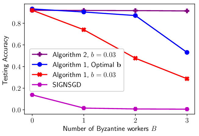
Figure 2: The left and right figures show the testing accuracy of Sto-SIGNSGD for different number of Byzantine workers and different 𝒃\boldsymbol{b} on MNIST and CIFAR-10, respectively. For MNIST, the Byzantine workers evaluate their gradients over the whole training dataset. For CIFAR-10, each Byzantine worker has 2,000 training examples that are sampled from the training dataset uniformly at random. The mini-batch sizes of all the workers and the Byzantine attackers are set to 32.

Experimental results. Fig. 2 shows the performance of Sto-SIGNSGD for different selection of 𝒃=b⋅𝟏\boldsymbol{b}=b\cdot\boldsymbol{1} and different number of Byzantine workers BB. It can be seen that as the number of Byzantine workers increases, both the training and the testing accuracy of Sto-SIGNSGD with a larger bb drop much faster than that with a smaller bb, which conforms to our analysis above that a lager bb results in worse Byzantine resilience. It is also observed that SIGNSGD essentially fails in this extremely heterogeneous data distribution setting (where each worker holds exclusive data), even without attackers.

Furthermore, to examine the impact of data heterogeneity, we vary the number of labels of each worker’s local training dataset in Table 1. It can be observed that the testing accuracy of SIGNSGD improves when the training data become more homogeneously distributed across workers. Furthermore, both SIGNSGD and Sto-SIGNSGD obtain better Byzantine resilience as the number of labels increases. Finally, Sto-SIGNSGD with optimal 𝒃\boldsymbol{b} still outperforms SIGNSGD, which indicates that introducing the stochasticity is still beneficial in the more homogeneous data distribution scenarios.

Table 1: Testing Accuracy of Sto-SIGNSGD on MNIST
BB SIGNSGD 2 Labels optimal 𝒃\boldsymbol{b} 2 Labels SIGNSGD 4 Labels optimal 𝒃\boldsymbol{b} 4 Labels
0 70.03% 92.34% 90.53% 93.12%
1 66.31% 93.14% 88.21% 93.38%
2 60.19% 92.71% 87.34% 93.39%
3 56.23% 91.13% 82.49% 92.19%
4 47.44% 84.49% 81.51% 92.31%

6 Improved Resilience with Weighted Vote

According to Theorem 7, it is shown that the number of Byzantine attackers that Sto-SIGNSGD can tolerate decreases as the gradient |∑m=1M∇fm​(w(t))||\sum_{m=1}^{M}\nabla f_{m}(w^{(t)})| decreases. As a result, Sto-SIGNSGD is more robust against Byzantine attackers in the beginning of the training process. With such consideration, a reputation based weighted vote mechanism is proposed and the corresponding algorithm is presented in Algorithm 2. In the proposed mechanism, the server stores a credit rm(t)r_{m}^{(t)} for each worker. During each iteration, given the shared signs of the gradients from the workers, the server first performs a weighted vote given by (17). Then, the aggregated result 𝒈~(t)\tilde{\boldsymbol{g}}^{(t)} is used as the “ground truth”, based on which a credit is assigned to each worker. More specifically, in (18), ∑i=1d𝟙𝒈~i(t)=q​(𝒈m(t))i/d\sum_{i=1}^{d}\mathds{1}_{\tilde{\boldsymbol{g}}^{(t)}_{i}=q(\boldsymbol{g}_{m}^{(t)})_{i}}/d and ∑i=1d𝟙𝒈~i(t)≠q​(𝒈m(t))i/d\sum_{i=1}^{d}\mathds{1}_{\tilde{\boldsymbol{g}}^{(t)}_{i}\neq q(\boldsymbol{g}_{m}^{(t)})_{i}}/d measures the number of coordinates that worker mm shares the same and different signs compared to the aggregated result, respectively. Considering that in the beginning of the training process, the probability of correct aggregation is high, and the attackers that deliberately share wrong signs are expected to receive lower credits and therefore play a smaller role in the future iterations. As a result, the impact of the attackers is reduced.

Algorithm 2 Stochastic-Sign SGD with weighted vote
 Input: learning rate η\eta, current hypothesis vector w(t)w^{(t)}, MM workers each with an independent gradient 𝒈m(t)\boldsymbol{g}_{m}^{(t)}, the 1-bit compressor q⁡(⋅)q(\cdot), initialized credit rm(0)=1,∀mr_{m}^{(0)}=1,\forall m.
 on server:
     pull q⁡(𝒈m(t))q(\boldsymbol{g}_{m}^{(t)}) from worker mm and compute the weighted vote given by
𝒈~(t)=s​i​g​n​(CLOSE​1M​∑m=1Mmax⁡{rm(t),0}​q​(𝒈m(t))​)\tilde{\boldsymbol{g}}^{(t)}=sign\hbox{$\left(\vbox to0.0pt{}\right.$}\frac{1}{M}\sum_{m=1}^{M}\max\{r_{m}^{(t)},0\}q(\boldsymbol{g}_{m}^{(t)})\hbox{$\left)\vbox to0.0pt{}\right.$} (17)
     push 𝒈~(t)\tilde{\boldsymbol{g}}^{(t)} to all the workers and update the credits
rm(t+1)=rm(t)+∑i=1d[𝟙𝒈~i(t)=q​(𝒈m(t))i−𝟙𝒈~i(t)≠q​(𝒈m(t))i]d,r_{m}^{(t+1)}=r_{m}^{(t)}+\frac{\sum_{i=1}^{d}[\mathds{1}_{\tilde{\boldsymbol{g}}^{(t)}_{i}=q(\boldsymbol{g}_{m}^{(t)})_{i}}-\mathds{1}_{\tilde{\boldsymbol{g}}^{(t)}_{i}\neq q(\boldsymbol{g}_{m}^{(t)})_{i}}]}{d}, (18)
where 𝒈~i(t)\tilde{\boldsymbol{g}}^{(t)}_{i} and q​(𝒈m(t))iq(\boldsymbol{g}_{m}^{(t)})_{i} are the ii-th entry of the aggregated result 𝒈~(t)\tilde{\boldsymbol{g}}^{(t)} and the vector q⁡(𝒈m(t))q(\boldsymbol{g}_{m}^{(t)}) shared by worker mm, respectively.
 on each worker:
     update w(t+1)=w(t)−η​𝒈~(t)w^{(t+1)}=w^{(t)}-\eta\tilde{\boldsymbol{g}}^{(t)}.
Refer to caption
Refer to caption
Figure 3: The left figure shows the testing accuracy of Sto-SIGNSGD with weighted vote on MNIST with 𝒃=0.03⋅𝟏\boldsymbol{b}=0.03\cdot\boldsymbol{1} and different number of Byzantine workers that evaluate their gradients over the whole training dataset. The right figure shows the testing accuracy of Sto-SIGNSGD with weighted vote on CIFAR-10, with 𝒃=0.012⋅𝟏\boldsymbol{b}=0.012\cdot\boldsymbol{1}. Each Byzantine worker has 2,000 training examples that are sampled from the training dataset uniformly at random. The mini-batch sizes of all the workers and the Byzantine attackers are set to 32.

Experimental results. Fig. 3 shows the performance of Sto-SIGNSGD with weighted vote. It can be observed that for MNIST, Sto-SIGNSGD with weighted vote obtains a comparable testing accuracy in the presence of up to 3 Byzantine workers compared to Sto-SIGNSGD without Byzantine workers. For CIFAR-10, it can be observed that Sto-SIGNSGD diverges in the presence of 5 Byzantine attackers. In the meantime, Sto-SIGNSGD with weighted vote achieves almost the same testing accuracy against 5 Byzantine workers as Sto-SIGNSGD without Byzantine workers. Furthermore, Sto-SIGNSGD with weighted vote achieves a higher testing accuracy against 10 Byzantine workers compared to Sto-SIGNSGD against 1 Byzantine worker, which validates its effectiveness.

7 Improved Differential Privacy with Sparsification

Intuitively, according to Theorem 6, as the absolute value of the true gradient |∇F(w(t))i||\nabla F(w^{(t)})_{i}| decreases, the corresponding probability of wrong aggregation increases. In this sense, discarding the coordinates with higher probabilities of wrong aggregation may help improve the learning performance. Therefore, we propose to improve the performance of DP-SIGNSGD by incorporating the Top-K sparsification scheme [35, 36]. The corresponding algorithm is termed as DP-TopSIGNSGD and presented in Algorithm 3.

Algorithm 3 DP-SIGNSGD with sparsification
 Input: learning rate η\eta, current hypothesis vector w(t)w^{(t)}, MM workers each with an independent gradient 𝒈m(t)\boldsymbol{g}_{m}^{(t)}, the 1-bit compressor q⁡(⋅)q(\cdot), the Top-kk sparsifier t​o​pk​(⋅)top_{k}(\cdot).
 on server:
   pull d​p​-​s​i​g​n​(t​o​pk​(𝒈m(t)))dp\text{-}sign(top_{k}(\boldsymbol{g}_{m}^{(t)})) from worker mm.
   push 𝒈~(t)=s​i​g​n​(CLOSE​1M​∑m=1Md​p​-​s​i​g​n​(t​o​pk​(𝒈m(t)))​)\tilde{\boldsymbol{g}}^{(t)}=sign\hbox{$\left(\vbox to0.0pt{}\right.$}\frac{1}{M}\sum_{m=1}^{M}dp\text{-}sign(top_{k}(\boldsymbol{g}_{m}^{(t)}))\hbox{$\left)\vbox to0.0pt{}\right.$} to all the workers.
 on each worker:
   update w(t+1)=w(t)−η​𝒈~(t)w^{(t+1)}=w^{(t)}-\eta\tilde{\boldsymbol{g}}^{(t)}.

Experimental results. We compare our proposed differentially private scheme with DP-FedSGD [37], a direct extension of DP-SGD [38] to the distributed setting, where differential privacy is provided through additive Gaussian noise. Moreover, we further incorporate the Top-K sparsification scheme [35, 36] into DP-SIGNSGD. In this case, each client only sends 10% of the coordinates of the gradients with the largest magnitudes through the d​p​-​s​i​g​ndp\text{-}sign compressor, and the corresponding algorithm is termed as DP-TopSIGNSGD. The corresponding results are presented in Fig. 4, where we run the algorithms for 200 communication rounds and utilize the notion of Gaussian differential privacy for privacy composition [39]. We set σ∈{10,20,30,50,80}\sigma\in\{10,20,30,50,80\}, which provide μ\mu-Gaussian differential privacy guarantees of μ∈{5.66,2.83,1.89,1.13,0.71}\mu\in\{5.66,2.83,1.89,1.13,0.71\}; in terms of common notion of differential privacy, this corresponds to ϵ∈{4.05,1.48,0.83,0.38,0.18}\epsilon\in\{4.05,1.48,0.83,0.38,0.18\} for the commonly considered δ=10−5\delta=10^{-5}.44 4 Essentially, a mechanism is μ\mu-Gaussian differential privacy if and only if it is (ϵ,δ⁡(ϵ))(\epsilon,\delta(\epsilon))-differential privacy with δ⁡(ϵ)=Φ⁡(−ϵμ+μ2)−eϵ​Φ​(−ϵμ−μ2)\delta(\epsilon)=\Phi(-\frac{\epsilon}{\mu}+\frac{\mu}{2})-e^{\epsilon}\Phi(-\frac{\epsilon}{\mu}-\frac{\mu}{2}). It can be seen that DP-SIGNSGD performs similarly with DP-FedSGD for the same level of privacy protection, while enjoying an improvement of 32×32\times in communication efficiency. DP-TopSIGNSGD outperforms DP-FedSGD and the improvement increases as σ\sigma increases (which indicates more stringent requirement for privacy), while further reduces the communication overhead (compared to DP-SIGNSGD).

Refer to caption
Figure 4: Performance of DP-TopSIGNSGD, DP-SIGNSGD and DP-FedSGD on MNIST. We follow the idea of gradient clipping in [38] to bound the sensitivity Δ2\Delta_{2}. After computing the gradient for each individual training sample in the local dataset, each worker clips it in its L2L_{2} norm for a clipping threshold CC to ensure that Δ2≤C\Delta_{2}\leq C. We set C=4C=4 in the experiments.

8 Extending to SGD

Up until this point in the paper, the discussions are based on the assumption that each worker can evaluate its local true gradient ∇fm​(w(t))\nabla f_{m}(w^{(t)}) for the ease of presentation. In the SGD scenario, we have to further account for the sampling noise. Particularly, the following theorem for Sto-SIGNSGD can be proved. The corresponding result for DP-SIGNSGD can be obtained following a similar strategy.

Theorem 8.

Suppose Assumptions 1-4 are satisfied, and set the learning rate η=1T​d\eta=\frac{1}{\sqrt{Td}}. Then, when 𝐛=b⋅𝟏\boldsymbol{b}=b\cdot\boldsymbol{1} and bb is sufficiently large, Sto-SIGNSGD converges to the (local) optimum if either of the following two conditions is satisfied.

  • •

    P(CLOSEsign(1M∑m=1M(𝒈mt)i)≠sign(∇F(wt)i)<0.5,∀1≤i≤dP\hbox{$\left(\vbox to0.0pt{}\right.$}sign(\frac{1}{M}\sum_{m=1}^{M}(\boldsymbol{g}_{m}^{t})_{i})\neq sign(\nabla F(w^{t})_{i}\hbox{$\left)\vbox to0.0pt{}\right.$}<0.5,\forall 1\leq i\leq d.

  • •

    The mini-batch size of stochastic gradient at each iteration is at least TT.

Remark 8.

Note that the first condition is not hard to satisfy. One sufficient condition is that the sampling noise of each worker is symmetric with zero mean. This assumption is also used in [8], which shows that the sampling noise is approximately not only symmetric, but also unimodal.

Remark 9.

We note that the above discussion assumes that bb is sufficiently large, which guarantees that the probability of wrong aggregation is less than 0.5. For an arbitrary bb that satisfies the condition in the definition of s​t​o​-​s​i​g​nsto\text{-}sign, we believe that it is possible to prove that the algorithm converges to the neighborhood of the (local) optimum. In particular, similar to the proof of Theorem 2, there will be an additional term ∑i=1d|∇F(wt)i|𝟙|1M​∑m=1M(𝐠mt)i|≤b​Δ​(M)\sum_{i=1}^{d}|\nabla F(w^{t})_{i}|\mathds{1}_{|\frac{1}{M}\sum_{m=1}^{M}(\boldsymbol{g}_{m}^{t})_{i}|\leq b\Delta(M)}. It is possible to upper bound this additional term given the fact that 𝔼[1M∑m=1M(𝐠mt)i]=∇F(wt)i\mathbb{E}[\frac{1}{M}\sum_{m=1}^{M}(\boldsymbol{g}_{m}^{t})_{i}]=\nabla F(w^{t})_{i}, despite that more efforts are required to make the analysis rigorous.

9 Extending to Error-feedback Variant

To further improved the performance of Algorithm 1, we incorporate the error-feedback technique and propose its error-feedback variant (i.e., Algorithm 4), where the server utilizes an α\alpha-approximate compressor 𝒞⁡(⋅)\mathcal{C}(\cdot) (i.e., ‖𝒞⁡(𝒙)−𝒙‖22≤(1−α)​‖𝒙‖22,∀𝒙||\mathcal{C}(\boldsymbol{x})-\boldsymbol{x}||_{2}^{2}\leq(1-\alpha)||\boldsymbol{x}||_{2}^{2},\forall\boldsymbol{x} [21]) and keeps track of the corresponding compression error.

Algorithm 4 Error-Feedback Stochastic-Sign SGD with majority vote
 Input: learning rate η\eta, current hypothesis vector w(t)w^{(t)}, current residual error vector 𝒆~(t)\tilde{\boldsymbol{e}}^{(t)}, MM workers each with an independent gradient 𝒈m(t)=∇fm​(w(t))\boldsymbol{g}_{m}^{(t)}=\nabla f_{m}(w^{(t)}), the 1-bit compressor q⁡(⋅)q(\cdot).
 on server:
     pull q⁡(𝒈m(t))q(\boldsymbol{g}_{m}^{(t)}) from worker mm.
     push 𝒈~(t)=𝒞​(CLOSE​1M​∑m=1Mq⁡(𝒈m(t))+𝒆~(t)​)\tilde{\boldsymbol{g}}^{(t)}=\mathcal{C}\hbox{$\left(\vbox to0.0pt{}\right.$}\frac{1}{M}\sum_{m=1}^{M}q(\boldsymbol{g}_{m}^{(t)})+\tilde{\boldsymbol{e}}^{(t)}\hbox{$\left)\vbox to0.0pt{}\right.$} to all the workers,
     update residual error:
𝒆~(t+1)=1M​∑m=1Mq⁡(𝒈m(t))+𝒆~(t)−𝒈~(t).\tilde{\boldsymbol{e}}^{(t+1)}=\frac{1}{M}\sum_{m=1}^{M}q(\boldsymbol{g}_{m}^{(t)})+\tilde{\boldsymbol{e}}^{(t)}-\tilde{\boldsymbol{g}}^{(t)}. (19)
 on each worker:
     update w(t+1)=w(t)−η​𝒈~(t)w^{(t+1)}=w^{(t)}-\eta\tilde{\boldsymbol{g}}^{(t)}.
Remark 10.

Note that in Algorithm 4, only the server adopts the error-feedback method. When d​p​-​s​i​g​ndp\text{-}sign is used, implementing error-feedback on the worker’s side may increase the privacy leakage. Accounting for the additional privacy leakage caused by error-feedback is left as future work.

Both s​t​o​-​s​i​g​nsto\text{-}sign and d​p​-​s​i​g​ndp\text{-}sign can be used in Algorithm 4 and the corresponding algorithms are termed as EF-Sto-SIGNSGD and EF-DP-SIGNSGD, respectively. In the following, we show the convergence and Byzantine resilience of Algorithm 4 when s​t​o​-​s​i​g​nsto\text{-}sign is used. The results can be easily adapted for d​p​-​s​i​g​ndp\text{-}sign. Particularly, the following theorems can be proved.

Theorem 9.

When Assumptions 1, 2 and 4 are satisfied, by running Algorithm 4 with η=1T​d\eta=\frac{1}{\sqrt{Td}}, q⁡(𝐠m(t))=s​t​o​-​s​i​g​n​(∇fm​(w(t)),𝐛)q(\boldsymbol{g}_{m}^{(t)})=sto\text{-}sign(\nabla f_{m}(w^{(t)}),\boldsymbol{b}) and 𝐛=b⋅𝟏\boldsymbol{b}=b\cdot\boldsymbol{1}, we have

1T​∑t=0T−1‖∇F​(w(t))‖22b≤(F⁡(w0)−F∗)​dT+(1+L+L2​β)​dT,\begin{split}\frac{1}{T}\sum_{t=0}^{T-1}\frac{||\nabla F(w^{(t)})||^{2}_{2}}{b}&\leq\frac{(F(w_{0})-F^{*})\sqrt{d}}{\sqrt{T}}+\frac{(1+L+L^{2}\beta)\sqrt{d}}{\sqrt{T}},\end{split} (20)

where β\beta is some positive constant.

Remark 11.

Theorem 9 shows that if bib_{i}’s are upper bounded (i.e., when |∇fm(w(t))i|≤Q,∀m,t,i|\nabla f_{m}(w^{(t)})_{i}|\leq Q,\forall m,t,i as in [9]), EF-Sto-SIGNSGD can converge to the (local) optimum while Sto-SIGNSGD only converges to the neighborhood of optimum (c.f. Theorem 2).

In our experiments, the server adopts the compressor 𝒞⁡(𝐱)=1M​s​i​g​n​(𝐱)\mathcal{C}(\boldsymbol{x})=\frac{1}{M}sign(\boldsymbol{x}). In this case, the communication overhead of EF-Sto-SIGNSGD is essentially the same as Sto-SIGNSGD. Utilizing the fact that the output of the compressor q⁡(⋅)∈{−1,1}q(\cdot)\in\{-1,1\}, it can be readily shown that ‖1M​s​i​g​n​(𝐱)−𝐱‖22<‖𝐱‖22||\frac{1}{M}sign(\boldsymbol{x})-\boldsymbol{x}||_{2}^{2}<||\boldsymbol{x}||_{2}^{2} with 𝐱=1M​∑m=1Mq⁡(𝐠m(t))+𝐞~(t)\boldsymbol{x}=\frac{1}{M}\sum_{m=1}^{M}q(\boldsymbol{g}_{m}^{(t)})+\tilde{\boldsymbol{e}}^{(t)}, which suggests that there exists some α\alpha such that 𝒞⁡(⋅)\mathcal{C}(\cdot) is α\alpha-approximate compressor. More details can be found in Section 4 of the supplementary document.

Besides the fact that error-feedback is only used on the server’s side, another difference between Algorithm 4 and those in [21, 22] is that it does not require the workers to share the magnitude information about the gradients. On the one hand, it saves communication overhead. On the other hand, it keeps the resilience against the re-scaling attacks. By following a similar strategy to the proofs of Theorem 9 and considering the impact of Byzantine attackers, we obtain the Byzantine resilience of Algorithm 4 as follows.

Theorem 10.

At each iteration tt, Algorithm 4 can at least tolerate ki=|∑m=1M∇fm(w(t))i|/bk_{i}=|\sum_{m=1}^{M}\nabla f_{m}(w^{(t)})_{i}|/b Byzantine attackers on the ii-th coordinate of the gradient. Overall, the number of Byzantine workers that Algorithm 4 can tolerate is given by m​i​n1≤i≤d​kimin_{1\leq i\leq d}k_{i}.

Refer to caption
Refer to caption
Refer to caption
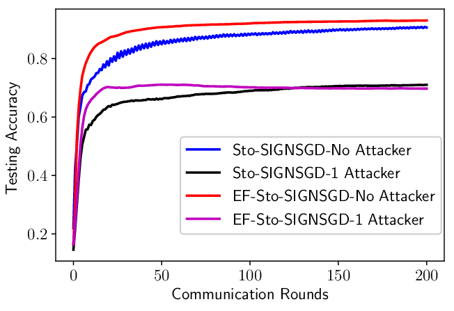
Figure 5: The first figure shows the performance of DP-SIGNSGD and EF-DP-SIGNSGD on MNIST for different ϵ\epsilon when δ=10−5\delta=10^{-5}, without Byzantine attackers. The ϵ\epsilon’s measure the per epoch privacy guarantee of the algorithms. The second figure compares Sto-SIGNSGD with EF-Sto-SIGNSGD on MNIST with 𝒃=0.02⋅𝟏\boldsymbol{b}=0.02\cdot\boldsymbol{1}. The last figure compares Sto-SIGNSGD with EF-Sto-SIGNSGD on CIFAR-10 with optimal 𝒃\boldsymbol{b}.

Experimental results. For DP-SIGNSGD and EF-DP-SIGNSGD, we follow the idea of gradient clipping in [38] to bound the sensitivity Δ2\Delta_{2}. After computing the gradient for each individual training sample in the local dataset, each worker clips it in its L2L_{2} norm for a clipping threshold CC to ensure that Δ2≤C\Delta_{2}\leq C. We set C=4C=4 in the experiments and the results are shown in the first figure of Fig. 5. It can be observed that when there is no Byzantine attackers, EF-DP-SIGNSGD outperforms DP-SIGNSGD for all the examined ϵ\epsilon’s, which demonstrates its effectiveness.

Another observation is that the error-feedback variants do not necessarily perform better. For instance, in the last figure of Fig. 5, when there are 3 Byzantine attackers, the testing accuracy of EF-Sto-SIGNSGD is worse than that of Sto-SIGNSGD. In the beginning of the training process, kik_{i}’s in Theorem 10 are large enough such that the algorithm can tolerate the Byzantine attacker. As the gradients decrease, the probability of wrong aggregation increases. In this case, the error-feedback mechanism may carry the wrong aggregations to the future iterations and have a negative impact on the learning process.

10 Conclusion

We propose a Stochastic-Sign SGD framework which utilizes two novel gradient compressors and can deal with heterogeneous data distribution. The proposed algorithms are proved to converge in the heterogeneous data distribution scenario with the same rate as SIGNSGD in the homogeneous data distribution case. In particular, the proposed differentially private compressor d​p​-​s​i​g​ndp\text{-}sign improves the privacy and the accuracy simultaneously without sacrificing any communication efficiency. Then, we further improve the learning performance of the proposed method by incorporating the error-feedback scheme. In addition, the Byzantine resilience of the proposed algorithms is shown analytically. It is expected that the proposed algorithms can find wide applications in the design of communication efficient, differentially private and Byzantine resilient FL algorithms.

Supplementary Material

The supplementary material is organized as follows. In Section 1, we formally provide the definition of local differential privacy [10]. In Section 2, we provide the proofs of the theoretical results presented in the main document. Discussions about the extended differentially private compressor d​p​-​s​i​g​ndp\text{-}sign when δ=0\delta=0 are provided in Section 3. Discussions about the server’s compressor 𝒞⁡(⋅)\mathcal{C}(\cdot) in Algorithm 4 are provided in Section 4. The details about the implementation of our experiments and some additional experimental results are presented in Section 5.

1 Definition of Local Differential Privacy

In this work, we study the privacy guarantee of the proposed algorithms from the lens of local differential privacy [10], which provides a strong notion of individual privacy in data analysis. The definition of local differential privacy is formally given as follows.

Definition 3.

Given a set of local datasets 𝒟\mathcal{D} provided with a notion of neighboring local datasets 𝒩𝒟⊂𝒟×𝒟\mathcal{N}_{\mathcal{D}}\subset\mathcal{D}\times\mathcal{D} that differ in only one data point. For a query function f:𝒟→𝒳f:\mathcal{D}\rightarrow\mathcal{X}, a mechanism ℳ:𝒳→𝒪\mathcal{M}:\mathcal{X}\rightarrow\mathcal{O} to release the answer of the query is defined to be (ϵ,δ)(\epsilon,\delta)-locally differentially private if for any measurable subset 𝒮⊆𝒪\mathcal{S}\subseteq\mathcal{O} and two neighboring local datasets (D1,D2)∈𝒩𝒟(D_{1},D_{2})\in\mathcal{N}_{\mathcal{D}},

P⁡(ℳ⁡(f⁡(D1))∈𝒮)≤eϵ​P​(ℳ⁡(f⁡(D2))∈𝒮)+δ.P(\mathcal{M}(f(D_{1}))\in\mathcal{S})\leq e^{\epsilon}P(\mathcal{M}(f(D_{2}))\in\mathcal{S})+\delta. (21)

A key quantity in characterizing local differential privacy for many mechanisms is the sensitivity of the query ff in a given norm lrl_{r}, which is defined as

Δr=max(D1,D2)∈𝒩𝒟⁡‖f⁡(D1)−f⁡(D2)‖r.\Delta_{r}=\max_{(D_{1},D_{2})\in\mathcal{N}_{\mathcal{D}}}||f(D_{1})-f(D_{2})||_{r}. (22)

For more details about the concept of differential privacy, the reader is referred to [10] for a survey.

2 Proofs

2.1 Proof of Theorem 1

Theorem 1.

Let u1,u2,⋯,uMu_{1},u_{2},\cdots,u_{M} be MM known and fixed real numbers and consider binary random variables u^m\hat{u}_{m}, 1≤m≤M1\leq m\leq M. Suppose that p¯=1M​∑m=1MPr⁡(s​i​g​n​(1M​∑m=1Mum)≠u^m)<12\bar{p}=\frac{1}{M}\sum_{m=1}^{M}\Pr\left(sign\left(\frac{1}{M}\sum_{m=1}^{M}u_{m}\right)\neq\hat{u}_{m}\right)<\frac{1}{2}, we have

P​(CLOSE​s​i​g​n​(CLOSE​1M​∑m=1Mu^m​)≠s​i​g​n​(CLOSE​1M​∑m=1Mum​))≤[​4​p¯​(1−p¯)​]M2,\begin{split}P\hbox{$\left(\vbox to0.0pt{}\right.$}sign\hbox{$\left(\vbox to0.0pt{}\right.$}\frac{1}{M}\sum_{m=1}^{M}\hat{u}_{m}\hbox{$\left)\vbox to0.0pt{}\right.$}&\neq sign\hbox{$\left(\vbox to0.0pt{}\right.$}\frac{1}{M}\sum_{m=1}^{M}u_{m}\hbox{$\left)\vbox to0.0pt{}\right.$}\hbox{$\left)\vbox to0.0pt{}\right.$}\leq\hbox{$\left[\vbox to0.0pt{}\right.$}4\bar{p}(1-\bar{p})\hbox{$\left]\vbox to0.0pt{}\right.$}^{\frac{M}{2}},\end{split} (23)
Proof.

Define a series of random variables {Xm}m=1M\{X_{m}\}_{m=1}^{M} given by

Xm={1,if u^m≠s​i​g​n​(CLOSE​1M​∑m=1Mum​),−1,if u^m=s​i​g​n​(CLOSE​1M​∑m=1Mum​).X_{m}=\begin{cases}\hfill 1,\hfill&\text{if $\hat{u}_{m}\neq sign\hbox{$\left(\vbox to0.0pt{}\right.$}\frac{1}{M}\sum_{m=1}^{M}u_{m}\hbox{$\left)\vbox to0.0pt{}\right.$}$},\\ \hfill-1,\hfill&\text{if $\hat{u}_{m}=sign\hbox{$\left(\vbox to0.0pt{}\right.$}\frac{1}{M}\sum_{m=1}^{M}u_{m}\hbox{$\left)\vbox to0.0pt{}\right.$}$.}\end{cases} (24)

In particular, XmX_{m} can be considered as the outcome of one Bernoulli trial with successful probability P⁡(Xm=1)P(X_{m}=1), and we have

P​(CLOSE​s​i​g​n​(CLOSE​1M​∑m=1Mu^m​)≠s​i​g​n​(CLOSE​1M​∑m=1Mum​))=P⁡(∑m=1MXm≥0).P\hbox{$\left(\vbox to0.0pt{}\right.$}sign\hbox{$\left(\vbox to0.0pt{}\right.$}\frac{1}{M}\sum_{m=1}^{M}\hat{u}_{m}\hbox{$\left)\vbox to0.0pt{}\right.$}\neq sign\hbox{$\left(\vbox to0.0pt{}\right.$}\frac{1}{M}\sum_{m=1}^{M}u_{m}\hbox{$\left)\vbox to0.0pt{}\right.$}\hbox{$\left)\vbox to0.0pt{}\right.$}=P\left(\sum_{m=1}^{M}X_{m}\geq 0\right). (25)

For any variable a>0a>0, we have

P⁡(∑m=1MXm≥0)=P⁡(ea​∑m=1MXm≥e0)≤𝔼⁡[ea​∑m=1MXm]e0=𝔼⁡[ea​∑m=1MXm],\begin{split}P\left(\sum_{m=1}^{M}X_{m}\geq 0\right)=P\left(e^{a\sum_{m=1}^{M}X_{m}}\geq e^{0}\right)&\leq\frac{\mathbb{E}[e^{a\sum_{m=1}^{M}X_{m}}]}{e^{0}}=\mathbb{E}[e^{a\sum_{m=1}^{M}X_{m}}],\end{split} (26)

which is due to Markov’s inequality, given the fact that ea​∑m=1MXme^{a\sum_{m=1}^{M}X_{m}} is non-negative. For the ease of presentation, let P⁡(Xm=1)=pmP(X_{m}=1)=p_{m}, we have,

𝔼⁡[ea​∑m=1MXm]=eln⁡(𝔼⁡[ea​∑m=1MXm])=eln⁡(∏m=1M𝔼⁡[ea​Xm])=e∑m=1Mln⁡(𝔼⁡[ea​Xm])=e∑m=1Mln⁡(ea​pm+e−a​(1−pm))=eM⁡(1M​∑m=1Mln⁡(ea​pm+e−a​(1−pm)))≤eM​ln⁡(ea​p¯+e−a​(1−p¯)),\begin{split}\mathbb{E}[e^{a\sum_{m=1}^{M}X_{m}}]&=e^{\ln(\mathbb{E}[e^{a\sum_{m=1}^{M}X_{m}}])}=e^{\ln(\prod_{m=1}^{M}\mathbb{E}[e^{aX_{m}}])}=e^{\sum_{m=1}^{M}\ln(\mathbb{E}[e^{aX_{m}}])}\\ &=e^{\sum_{m=1}^{M}\ln(e^{a}p_{m}+e^{-a}(1-p_{m}))}\\ &=e^{M\left(\frac{1}{M}\sum_{m=1}^{M}\ln(e^{a}p_{m}+e^{-a}(1-p_{m}))\right)}\\ &\leq e^{M\ln(e^{a}\bar{p}+e^{-a}(1-\bar{p}))},\end{split} (27)

where p¯=1M​∑m=1Mpm\bar{p}=\frac{1}{M}\sum_{m=1}^{M}p_{m} and the inequality is due to Jensen’s inequality. Optimizing aa yields a=ln⁡(1−p¯p¯)>0a=\ln\left(\sqrt{\frac{1-\bar{p}}{\bar{p}}}\right)>0 and

eM​ln⁡(ea​p¯+e−a​(1−p¯))=[4​p¯​(1−p¯)]M2,e^{M\ln(e^{a}\bar{p}+e^{-a}(1-\bar{p}))}=[4\bar{p}(1-\bar{p})]^{\frac{M}{2}}, (28)

which completes the proof. ∎

2.2 Proof of Corollary 1

Corollary 1.

Let u1,u2,⋯,uMu_{1},u_{2},\cdots,u_{M} be MM known and fixed real numbers and consider binary random variables u^m=s​t​o​-​s​i​g​n​(um,b)\hat{u}_{m}=sto\text{-}sign(u_{m},b), 1≤m≤M1\leq m\leq M. We have p¯=1M​∑m=1MPr⁡(s​i​g​n​(1M​∑m=1Mum)≠u^m)=b​M−|∑m=1Mum|2​b​M\bar{p}=\frac{1}{M}\sum_{m=1}^{M}\Pr\left(sign\left(\frac{1}{M}\sum_{m=1}^{M}u_{m}\right)\neq\hat{u}_{m}\right)=\frac{bM-|\sum_{m=1}^{M}u_{m}|}{2bM}, and

P​(CLOSE​s​i​g​n​(CLOSE​1M​∑m=1Mu^m​)≠s​i​g​n​(CLOSE​1M​∑m=1Mum​))≤(1−x2)M2,\begin{split}P\hbox{$\left(\vbox to0.0pt{}\right.$}sign\hbox{$\left(\vbox to0.0pt{}\right.$}\frac{1}{M}\sum_{m=1}^{M}\hat{u}_{m}\hbox{$\left)\vbox to0.0pt{}\right.$}&\neq sign\hbox{$\left(\vbox to0.0pt{}\right.$}\frac{1}{M}\sum_{m=1}^{M}u_{m}\hbox{$\left)\vbox to0.0pt{}\right.$}\hbox{$\left)\vbox to0.0pt{}\right.$}\leq\left(1-x^{2}\right)^{\frac{M}{2}},\end{split} (29)

where x=|∑m=1Mum|b​Mx=\frac{|\sum_{m=1}^{M}u_{m}|}{bM}.

Proof.

It can be easily shown that p¯=1M​∑m=1MPr⁡(s​i​g​n​(1M​∑m=1Mum)≠u^m)=b​M−|∑m=1Mum|2​b​M\bar{p}=\frac{1}{M}\sum_{m=1}^{M}\Pr\left(sign\left(\frac{1}{M}\sum_{m=1}^{M}u_{m}\right)\neq\hat{u}_{m}\right)=\frac{bM-|\sum_{m=1}^{M}u_{m}|}{2bM} when u^m=s​t​o​-​s​i​g​n​(um,b)\hat{u}_{m}=sto\text{-}sign(u_{m},b). Plugging it into (23) completes the proof. ∎

2.3 Proof of Theorem 2

Theorem 2.

Suppose Assumptions 1, 2 and 4 are satisfied, and the learning rate is set as η=1T​d\eta=\frac{1}{\sqrt{Td}}. Then by running Sto-SIGNSGD for TT iterations, we have

1T​∑t=1T‖∇F​(w(t))‖1≤1c[𝔼⁡[F⁡(w(0))−F⁡(w(T+1))]​dT+L​d2​T+2​ηT∑t=1T∑i=1d|∇F(w(t))i|𝟙pi(t)>1−c2]≤1c​[​(F⁡(w(0))−F∗)​dT+L​d2​T+2​∑i=1dbi​Δ​(M)​],\color[rgb]{0,0,0}\begin{split}&\frac{1}{T}\sum_{t=1}^{T}||\nabla F(w^{(t)})||_{1}\\ &\leq\frac{1}{c}\hbox{$\left[\vbox to0.0pt{}\right.$}\frac{\mathbb{E}[F(w^{(0)})-F(w^{(T+1)})]\sqrt{d}}{\sqrt{T}}+\frac{L\sqrt{d}}{2\sqrt{T}}+\frac{2\eta}{T}\sum_{t=1}^{T}\sum_{i=1}^{d}|\nabla F(w^{(t)})_{i}|\mathds{1}_{p_{i}^{(t)}>\frac{1-c}{2}}\hbox{$\left]\vbox to0.0pt{}\right.$}\\ &\leq\frac{1}{c}\hbox{$\left[\vbox to0.0pt{}\right.$}\frac{(F(w^{(0)})-F^{*})\sqrt{d}}{\sqrt{T}}+\frac{L\sqrt{d}}{2\sqrt{T}}+2\sum_{i=1}^{d}b_{i}\Delta(M)\hbox{$\left]\vbox to0.0pt{}\right.$},\end{split} (30)

where 0<c<10<c<1 is some positive constant, pi(t)p_{i}^{(t)} is the probability that the aggregation on the ii-coordinate of the gradient is wrong during the tt-th communication round, and Δ⁡(M)\Delta(M) is the solution to (𝐶𝐿𝑂𝑆𝐸​1−x2​)M2=1−c2\hbox{$\left(\vbox to0.0pt{}\right.$}1-x^{2}\hbox{$\left)\vbox to0.0pt{}\right.$}^{\frac{M}{2}}=\frac{1-c}{2}. The second inequality is due to the fact that pi(t)>1−c2p_{i}^{(t)}>\frac{1-c}{2} only if |∇F(w(t))i|bi≤Δ⁡(M)\frac{|\nabla F(w^{(t)})_{i}|}{b_{i}}\leq\Delta(M).

The proof of Theorem 2 follows the well known strategy of relating the norm of the gradient to the expected improvement of the global objective in a single iteration. Then accumulating the improvement over the iterations yields the convergence rate of the algorithm.

Proof.

According to Assumption 2, we have

F⁡(w(t+1))−F⁡(w(t))≤<∇F(w(t)),w(t+1)−w(t)>+L2||w(t+1)−w(t)||2=−η⁡<∇F​(w(t)),s​i​g​n​(CLOSE​1M​∑m=1Ms​t​o​-​s​i​g​n​(𝒈m(t))​)>+L2​||​η​s​i​g​n​(CLOSE​1M​∑m=1Ms​t​o​-​s​i​g​n​(𝒈m(t))​)||2=−η⁡<∇F​(w(t)),s​i​g​n​(CLOSE​1M​∑m=1Ms​t​o​-​s​i​g​n​(𝒈m(t))​)>+L​η2​d2=−η||∇F(w(t))||1+L​η2​d2+2η∑i=1d|∇F(w(t))i|𝟙sign(1M∑m=1Msto-sign(𝒈m(t))i)≠sign(∇F(w(t))i),\begin{split}&F(w^{(t+1)})-F(w^{(t)})\\ &\leq<\nabla F(w^{(t)}),w^{(t+1)}-w^{(t)}>+\frac{L}{2}||w^{(t+1)}-w^{(t)}||^{2}\\ &=-\eta<\nabla F(w^{(t)}),sign\hbox{$\left(\vbox to0.0pt{}\right.$}\frac{1}{M}\sum_{m=1}^{M}sto\text{-}sign(\boldsymbol{g}_{m}^{(t)})\hbox{$\left)\vbox to0.0pt{}\right.$}>+\frac{L}{2}\hbox{$\left|\vbox to0.0pt{}\right.$}\hbox{$\left|\vbox to0.0pt{}\right.$}\eta sign\hbox{$\left(\vbox to0.0pt{}\right.$}\frac{1}{M}\sum_{m=1}^{M}sto\text{-}sign(\boldsymbol{g}_{m}^{(t)})\hbox{$\left)\vbox to0.0pt{}\right.$}\hbox{$\left|\vbox to0.0pt{}\right.$}\hbox{$\left|\vbox to0.0pt{}\right.$}^{2}\\ &=-\eta<\nabla F(w^{(t)}),sign\hbox{$\left(\vbox to0.0pt{}\right.$}\frac{1}{M}\sum_{m=1}^{M}sto\text{-}sign(\boldsymbol{g}_{m}^{(t)})\hbox{$\left)\vbox to0.0pt{}\right.$}>+\frac{L\eta^{2}d}{2}\\ &=-\eta||\nabla F(w^{(t)})||_{1}+\frac{L\eta^{2}d}{2}+2\eta\sum_{i=1}^{d}|\nabla F(w^{(t)})_{i}|\mathds{1}_{sign(\frac{1}{M}\sum_{m=1}^{M}sto\text{-}sign(\boldsymbol{g}_{m}^{(t)})_{i})\neq sign(\nabla F(w^{(t)})_{i})},\end{split} (31)

where ∇F(w(t))i\nabla F(w^{(t)})_{i} is the ii-th entry of the vector ∇F​(w(t))\nabla F(w^{(t)}) and η\eta is the learning rate. Taking expectation on both sides yeilds

𝔼⁡[F⁡(w(t+1))−F⁡(w(t))]≤−η​‖∇F​(w(t))‖1+L​η2​d2+2η∑i=1d|∇F(w(t))i|P(CLOSEsign(CLOSE1M∑m=1Msto-sign(𝒈m(t))i)≠sign(∇F(w(t))i))\color[rgb]{0,0,0}\begin{split}&\mathbb{E}[F(w^{(t+1)})-F(w^{(t)})]\leq-\eta||\nabla F(w^{(t)})||_{1}+\frac{L\eta^{2}d}{2}\\ &+2\eta\sum_{i=1}^{d}|\nabla F(w^{(t)})_{i}|P\hbox{$\left(\vbox to0.0pt{}\right.$}sign\hbox{$\left(\vbox to0.0pt{}\right.$}\frac{1}{M}\sum_{m=1}^{M}sto\text{-}sign(\boldsymbol{g}_{m}^{(t)})_{i}\hbox{$\left)\vbox to0.0pt{}\right.$}\neq sign(\nabla F(w^{(t)})_{i})\hbox{$\left)\vbox to0.0pt{}\right.$}\\ \end{split} (32)

Let Δ⁡(M)\Delta(M) denote the solution to [(CLOSE​1−x​)​ex​]M2=1−c2\hbox{$\left[\vbox to0.0pt{}\right.$}\hbox{$\left(\vbox to0.0pt{}\right.$}1-x\hbox{$\left)\vbox to0.0pt{}\right.$}e^{x}\hbox{$\left]\vbox to0.0pt{}\right.$}^{\frac{M}{2}}=\frac{1-c}{2}. Since (CLOSE​1−x​)​ex\hbox{$\left(\vbox to0.0pt{}\right.$}1-x\hbox{$\left)\vbox to0.0pt{}\right.$}e^{x} is a decreasing function of xx for 0<x<10<x<1, it can be verified that [(CLOSE​1−x​)​ex​]M2<1−c2\hbox{$\left[\vbox to0.0pt{}\right.$}\hbox{$\left(\vbox to0.0pt{}\right.$}1-x\hbox{$\left)\vbox to0.0pt{}\right.$}e^{x}\hbox{$\left]\vbox to0.0pt{}\right.$}^{\frac{M}{2}}<\frac{1-c}{2} when x>Δ⁡(M)x>\Delta(M) and [(CLOSE​1−x​)​ex​]M2≥1−c2\hbox{$\left[\vbox to0.0pt{}\right.$}\hbox{$\left(\vbox to0.0pt{}\right.$}1-x\hbox{$\left)\vbox to0.0pt{}\right.$}e^{x}\hbox{$\left]\vbox to0.0pt{}\right.$}^{\frac{M}{2}}\geq\frac{1-c}{2} otherwise. According to Theorem 1, we have two possible scenarios as follows.

P(CLOSEsign(CLOSE1M∑m=1Msto-sign(𝒈m(t))i)≠sign(∇F(w(t))i)){≤1−c2,if|∇F(w(t))i|bi>Δ(M),≤1,if|∇F(w(t))i|bi≤Δ(M).P\hbox{$\left(\vbox to0.0pt{}\right.$}sign\hbox{$\left(\vbox to0.0pt{}\right.$}\frac{1}{M}\sum_{m=1}^{M}sto\text{-}sign(\boldsymbol{g}_{m}^{(t)})_{i}\hbox{$\left)\vbox to0.0pt{}\right.$}\neq sign(\nabla F(w^{(t)})_{i})\hbox{$\left)\vbox to0.0pt{}\right.$}\begin{cases}\leq\frac{1-c}{2},\text{if}~\frac{|\nabla F(w^{(t)})_{i}|}{b_{i}}>\Delta(M),\\ \leq 1,\text{if}~\frac{|\nabla F(w^{(t)})_{i}|}{b_{i}}\leq\Delta(M).\end{cases} (33)

Plugging (33) into (32), we can obtain

𝔼⁡[F⁡(w(t+1))−F⁡(w(t))]≤−η​‖∇F​(w(t))‖1+L​η2​d2+η[(1−c)∑i=1d|∇F(w(t))i|𝟙pi(t)≤1−c2+(1−c)∑i=1d|∇F(w(t))i|𝟙pi(t)>1−c2]+2η∑i=1d|∇F(w(t))i|𝟙pi(t)>1−c2≤−η||∇F(w(t))||1+L​η2​d2+η(1−c)||∇F(w(t))||1+2η∑i=1d|∇F(w(t))i|𝟙pi(t)>1−c2=−ηc||∇F(w(t))||1+L​η2​d2+2η∑i=1d|∇F(w(t))i|𝟙pi(t)>1−c2,\color[rgb]{0,0,0}\begin{split}&\mathbb{E}[F(w^{(t+1)})-F(w^{(t)})]\\ &\leq-\eta||\nabla F(w^{(t)})||_{1}+\frac{L\eta^{2}d}{2}\\ &+\eta\hbox{$\left[\vbox to0.0pt{}\right.$}(1-c)\sum_{i=1}^{d}|\nabla F(w^{(t)})_{i}|\mathds{1}_{p_{i}^{(t)}\leq\frac{1-c}{2}}+(1-c)\sum_{i=1}^{d}|\nabla F(w^{(t)})_{i}|\mathds{1}_{p_{i}^{(t)}>\frac{1-c}{2}}\hbox{$\left]\vbox to0.0pt{}\right.$}\\ &+2\eta\sum_{i=1}^{d}|\nabla F(w^{(t)})_{i}|\mathds{1}_{p_{i}^{(t)}>\frac{1-c}{2}}\\ &\leq-\eta||\nabla F(w^{(t)})||_{1}+\frac{L\eta^{2}d}{2}+\eta(1-c)||\nabla F(w^{(t)})||_{1}+2\eta\sum_{i=1}^{d}|\nabla F(w^{(t)})_{i}|\mathds{1}_{p_{i}^{(t)}>\frac{1-c}{2}}\\ &=-\eta c||\nabla F(w^{(t)})||_{1}+\frac{L\eta^{2}d}{2}+2\eta\sum_{i=1}^{d}|\nabla F(w^{(t)})_{i}|\mathds{1}_{p_{i}^{(t)}>\frac{1-c}{2}},\end{split} (34)

where pi(t)=P(CLOSEsign(CLOSE1M∑m=1Msto-sign(𝒈m(t))i)≠sign(∇F(w(t))i))p_{i}^{(t)}=P\hbox{$\left(\vbox to0.0pt{}\right.$}sign\hbox{$\left(\vbox to0.0pt{}\right.$}\frac{1}{M}\sum_{m=1}^{M}sto\text{-}sign(\boldsymbol{g}_{m}^{(t)})_{i}\hbox{$\left)\vbox to0.0pt{}\right.$}\neq sign(\nabla F(w^{(t)})_{i})\hbox{$\left)\vbox to0.0pt{}\right.$} is the probability of wrong aggregation. Adjusting the above inequality and averaging both sides over t=1,2,⋯,Tt=1,2,\cdots,T, we can obtain

1T​∑t=1Tη​c​‖∇F​(w(t))‖1≤𝔼⁡[F⁡(w(0))−F⁡(w(T+1))]T+L​η2​d2+2​ηT∑t=1T∑i=1d|∇F(w(t))i|𝟙pi(t)>1−c2≤𝔼⁡[F⁡(w(0))−F⁡(w(T+1))]T+L​η2​d2+2​η​∑i=1dbi​Δ​(M),\color[rgb]{0,0,0}\begin{split}\frac{1}{T}\sum_{t=1}^{T}\eta c||\nabla F(w^{(t)})||_{1}&\leq\frac{\mathbb{E}[F(w^{(0)})-F(w^{(T+1)})]}{T}+\frac{L\eta^{2}d}{2}\\ &+\frac{2\eta}{T}\sum_{t=1}^{T}\sum_{i=1}^{d}|\nabla F(w^{(t)})_{i}|\mathds{1}_{p_{i}^{(t)}>\frac{1-c}{2}}\\ &\leq\frac{\mathbb{E}[F(w^{(0)})-F(w^{(T+1)})]}{T}+\frac{L\eta^{2}d}{2}+2\eta\sum_{i=1}^{d}b_{i}\Delta(M),\end{split} (35)

where the last inequality is due to the fact that pi(t)>1−c2p_{i}^{(t)}>\frac{1-c}{2} only when |∇F(w(t))i|bi≤Δ⁡(M)\frac{|\nabla F(w^{(t)})_{i}|}{b_{i}}\leq\Delta(M). Letting η=1d​T\eta=\frac{1}{\sqrt{dT}} and dividing both sides by c​ηc\eta gives

1T​∑t=1T‖∇F​(w(t))‖1≤1c[𝔼⁡[F⁡(w(0))−F⁡(w(T+1))]​dT+L​d2​T+2​ηT∑t=1T∑i=1d|∇F(w(t))i|𝟙pi(t)>1−c2]≤1c​[​(F⁡(w(0))−F∗)​dT+L​d2​T+2​∑i=1dbi​Δ​(M)​],\color[rgb]{0,0,0}\begin{split}&\frac{1}{T}\sum_{t=1}^{T}||\nabla F(w^{(t)})||_{1}\\ &\leq\frac{1}{c}\hbox{$\left[\vbox to0.0pt{}\right.$}\frac{\mathbb{E}[F(w^{(0)})-F(w^{(T+1)})]\sqrt{d}}{\sqrt{T}}+\frac{L\sqrt{d}}{2\sqrt{T}}+\frac{2\eta}{T}\sum_{t=1}^{T}\sum_{i=1}^{d}|\nabla F(w^{(t)})_{i}|\mathds{1}_{p_{i}^{(t)}>\frac{1-c}{2}}\hbox{$\left]\vbox to0.0pt{}\right.$}\\ &\leq\frac{1}{c}\hbox{$\left[\vbox to0.0pt{}\right.$}\frac{(F(w^{(0)})-F^{*})\sqrt{d}}{\sqrt{T}}+\frac{L\sqrt{d}}{2\sqrt{T}}+2\sum_{i=1}^{d}b_{i}\Delta(M)\hbox{$\left]\vbox to0.0pt{}\right.$},\end{split} (36)

which completes the proof. ∎

2.4 Proof of Theorem 3

Theorem 3.

Given Assumption 3 and the same {um}m=1M\{u_{m}\}_{m=1}^{M} and {u^m}m=1M\{\hat{u}_{m}\}_{m=1}^{M} as those in Theorem 1, we have

P​(CLOSE​s​i​g​n​(CLOSE​1M​∑m=1Mu^m​)≠s​i​g​n​(CLOSE​1M​∑m=1Mum​))=12−(M−1M−12)2M​b​|​∑m=1Mum​|+O​(CLOSE​1b2​)\begin{split}P\hbox{$\left(\vbox to0.0pt{}\right.$}sign\hbox{$\left(\vbox to0.0pt{}\right.$}\frac{1}{M}\sum_{m=1}^{M}\hat{u}_{m}\hbox{$\left)\vbox to0.0pt{}\right.$}\neq sign\hbox{$\left(\vbox to0.0pt{}\right.$}\frac{1}{M}\sum_{m=1}^{M}u_{m}\hbox{$\left)\vbox to0.0pt{}\right.$}\hbox{$\left)\vbox to0.0pt{}\right.$}=\frac{1}{2}-\frac{{M-1\choose\frac{M-1}{2}}}{2^{M}b}\hbox{$\left|\vbox to0.0pt{}\right.$}\sum_{m=1}^{M}u_{m}\hbox{$\left|\vbox to0.0pt{}\right.$}+O\hbox{$\left(\vbox to0.0pt{}\right.$}\frac{1}{b^{2}}\hbox{$\left)\vbox to0.0pt{}\right.$}\end{split} (37)
Proof.

Without loss of generality, assume u1≤u2≤⋯≤uK<0≤uK+1≤⋯≤uMu_{1}\leq u_{2}\leq\cdots\leq u_{K}<0\leq u_{K+1}\leq\cdots\leq u_{M}. According to the definition of s​t​o​-​s​i​g​nsto\text{-}sign, we have

u^m=s​t​o​-​s​i​g​n​(um,b)={1,with probability b+um2​b,−1,with probability b−um2​b,\hat{u}_{m}=sto\text{-}sign(u_{m},b)=\begin{cases}\hfill 1,\hfill\text{with probability $\frac{b+u_{m}}{2b}$},\\ \hfill-1,\hfill\text{with probability $\frac{b-u_{m}}{2b}$},\\ \end{cases} (38)

Further define a series of random variables {X^m}m=1M\{\hat{X}_{m}\}_{m=1}^{M} given by

X^m={1,if u^m=1,0,if u^m=−1.\hat{X}_{m}=\begin{cases}\hfill 1,\hfill&\text{if $\hat{u}_{m}=1$},\\ \hfill 0,\hfill&\text{if $\hat{u}_{m}=-1$.}\end{cases} (39)

In particular, X^m\hat{X}_{m} can be considered as the outcome of one Bernoulli trial with successful probability P⁡(X^m=1)P(\hat{X}_{m}=1). Let Z^=∑m=1MX^m\hat{Z}=\sum_{m=1}^{M}\hat{X}_{m}, then

P​(CLOSE​s​i​g​n​(CLOSE​1M​∑m=1Mu^m​)=1​)=P​(CLOSE​Z^≥M2​)=∑H=M+12MP⁡(Z^=H).P\hbox{$\left(\vbox to0.0pt{}\right.$}sign\hbox{$\left(\vbox to0.0pt{}\right.$}\frac{1}{M}\sum_{m=1}^{M}\hat{u}_{m}\hbox{$\left)\vbox to0.0pt{}\right.$}=1\hbox{$\left)\vbox to0.0pt{}\right.$}=P\hbox{$\left(\vbox to0.0pt{}\right.$}\hat{Z}\geq\frac{M}{2}\hbox{$\left)\vbox to0.0pt{}\right.$}=\sum_{H=\frac{M+1}{2}}^{M}P(\hat{Z}=H). (40)

In addition,

P⁡(Z^=H)=∑A∈FH∏i∈A(b+ui)​∏j∈Ac(b−uj)(2​b)M=aM,H​bM+aM−1,H​bM−1+⋯+a0,H​b0(2​b)M,P(\hat{Z}=H)=\frac{\sum_{A\in F_{H}}\prod_{i\in A}(b+u_{i})\prod_{j\in A^{c}}(b-u_{j})}{(2b)^{M}}=\frac{a_{M,H}b^{M}+a_{M-1,H}b^{M-1}+\cdots+a_{0,H}b^{0}}{(2b)^{M}}, (41)

in which FHF_{H} is the set of all subsets of HH integers that can be selected from {1,2,3,…,M}\{1,2,3,...,M\}; am,H,∀0≤m≤Ma_{m,H},\forall 0\leq m\leq M is some constant. It can be easily verified that aM,H=(MH)a_{M,H}={M\choose H}.

When bb is sufficiently large, P⁡(Z^=H)P(\hat{Z}=H) is dominated by the first two terms in (41). As a result, we have

P⁡(Z^=H)=aM,H​bM+aM−1,H​bM−1(2​b)M+O​(CLOSE​1b2​).P(\hat{Z}=H)=\frac{a_{M,H}b^{M}+a_{M-1,H}b^{M-1}}{(2b)^{M}}+O\hbox{$\left(\vbox to0.0pt{}\right.$}\frac{1}{b^{2}}\hbox{$\left)\vbox to0.0pt{}\right.$}. (42)

In particular, ∀m\forall m, we have

∑A∈FH∏i∈A(b+ui)​∏j∈Ac(b−uj)=(b+um)​∑A∈FH,m∈A∏i∈A/{m}(b+ui)​∏j∈Ac(b−uj)+(b−um)∑A∈FH,m∉A∏i∈A(b+ui)∏j∈Ac/{m}(b−uj).\begin{split}\sum_{A\in F_{H}}\prod_{i\in A}(b+u_{i})\prod_{j\in A^{c}}(b-u_{j})&=(b+u_{m})\sum_{A\in F_{H},m\in A}\prod_{i\in A/\{m\}}(b+u_{i})\prod_{j\in A^{c}}(b-u_{j})\\ &+(b-u_{m})\sum_{A\in F_{H},m\notin A}\prod_{i\in A}(b+u_{i})\prod_{j\in A^{c}/\{m\}}(b-u_{j}).\end{split} (43)

As a result, when M+12≤H≤M−1\frac{M+1}{2}\leq H\leq M-1, the umu_{m} related term in aM−1,Ha_{M-1,H} is given by

[​(M−1H−1)−(M−1H)​]​um.\hbox{$\left[\vbox to0.0pt{}\right.$}{M-1\choose H-1}-{M-1\choose H}\hbox{$\left]\vbox to0.0pt{}\right.$}u_{m}. (44)

When H=MH=M, the umu_{m} related term in aM−1,Ha_{M-1,H} is given by

[​(M−1H−1)​]​um.\hbox{$\left[\vbox to0.0pt{}\right.$}{M-1\choose H-1}\hbox{$\left]\vbox to0.0pt{}\right.$}u_{m}. (45)

By summing over mm, we have

aM−1,H=[​(M−1H−1)−(M−1H)​]​∑m=1Mum,if​M+12≤H≤M−1,a_{M-1,H}=\hbox{$\left[\vbox to0.0pt{}\right.$}{M-1\choose H-1}-{M-1\choose H}\hbox{$\left]\vbox to0.0pt{}\right.$}\sum_{m=1}^{M}u_{m},~~~~~\text{if}~~~\frac{M+1}{2}\leq H\leq M-1, (46)

and

aM−1,H=[​(M−1H−1)​]​∑m=1Mum,if​H=M.a_{M-1,H}=\hbox{$\left[\vbox to0.0pt{}\right.$}{M-1\choose H-1}\hbox{$\left]\vbox to0.0pt{}\right.$}\sum_{m=1}^{M}u_{m},~~~~~\text{if}~~~H=M. (47)

By summing over HH, we have

∑H=M+12MaM,H=∑H=M+12M(MH)=2M−1,\sum_{H=\frac{M+1}{2}}^{M}a_{M,H}=\sum_{H=\frac{M+1}{2}}^{M}{M\choose H}=2^{M-1}, (48)
∑H=M+12MaM−1,H=(M−1M−12)​∑m=1Mum.\sum_{H=\frac{M+1}{2}}^{M}a_{M-1,H}={M-1\choose\frac{M-1}{2}}\sum_{m=1}^{M}u_{m}. (49)

As a result,

P​(CLOSE​s​i​g​n​(CLOSE​1M​∑m=1Mu^m​)=1​)=P​(CLOSE​Z^≥M2​)=∑H=M+12MP⁡(Z^=H)=2M−1​bM+(M−1M−12)​∑m=1Mum​bM−1(2​b)M+O​(CLOSE​1b2​)=12+(M−1M−12)2M​b​∑m=1Mum+O​(CLOSE​1b2​).\begin{split}P\hbox{$\left(\vbox to0.0pt{}\right.$}sign\hbox{$\left(\vbox to0.0pt{}\right.$}\frac{1}{M}\sum_{m=1}^{M}\hat{u}_{m}\hbox{$\left)\vbox to0.0pt{}\right.$}=1\hbox{$\left)\vbox to0.0pt{}\right.$}&=P\hbox{$\left(\vbox to0.0pt{}\right.$}\hat{Z}\geq\frac{M}{2}\hbox{$\left)\vbox to0.0pt{}\right.$}\\ &=\sum_{H=\frac{M+1}{2}}^{M}P(\hat{Z}=H)\\ &=\frac{2^{M-1}b^{M}+{M-1\choose\frac{M-1}{2}}\sum_{m=1}^{M}u_{m}b^{M-1}}{(2b)^{M}}+O\hbox{$\left(\vbox to0.0pt{}\right.$}\frac{1}{b^{2}}\hbox{$\left)\vbox to0.0pt{}\right.$}\\ &=\frac{1}{2}+\frac{{M-1\choose\frac{M-1}{2}}}{2^{M}b}\sum_{m=1}^{M}u_{m}+O\hbox{$\left(\vbox to0.0pt{}\right.$}\frac{1}{b^{2}}\hbox{$\left)\vbox to0.0pt{}\right.$}.\end{split} (50)

Therefore,

P​(CLOSE​s​i​g​n​(CLOSE​1M​∑m=1Mu^m​)≠s​i​g​n​(CLOSE​1M​∑m=1Mum​))=12−(M−1M−12)2M​b​|​∑m=1Mum​|+O​(CLOSE​1b2​).\begin{split}P\hbox{$\left(\vbox to0.0pt{}\right.$}sign\hbox{$\left(\vbox to0.0pt{}\right.$}\frac{1}{M}\sum_{m=1}^{M}\hat{u}_{m}\hbox{$\left)\vbox to0.0pt{}\right.$}\neq sign\hbox{$\left(\vbox to0.0pt{}\right.$}\frac{1}{M}\sum_{m=1}^{M}u_{m}\hbox{$\left)\vbox to0.0pt{}\right.$}\hbox{$\left)\vbox to0.0pt{}\right.$}=\frac{1}{2}-\frac{{M-1\choose\frac{M-1}{2}}}{2^{M}b}\hbox{$\left|\vbox to0.0pt{}\right.$}\sum_{m=1}^{M}u_{m}\hbox{$\left|\vbox to0.0pt{}\right.$}+O\hbox{$\left(\vbox to0.0pt{}\right.$}\frac{1}{b^{2}}\hbox{$\left)\vbox to0.0pt{}\right.$}.\end{split} (51)

∎

2.5 Proof of Theorem 4

Theorem 4.

Suppose Assumptions 1, 2 and 4 are satisfied, |∇F(w(t))i|≤Q,∀1≤i≤d,1≤t≤T|\nabla F(w^{(t)})_{i}|\leq Q,\forall 1\leq i\leq d,1\leq t\leq T, and the learning rate is set as η=1T​d\eta=\frac{1}{\sqrt{Td}}. Then by running Algorithm 1 with q⁡(𝐠m(t))=s​t​o​-​s​i​g​n​(∇fm​(w(t)),𝐛)q(\boldsymbol{g}_{m}^{(t)})=sto\text{-}sign(\nabla f_{m}(w^{(t)}),\boldsymbol{b}) and bi=T1/4​d1/4,∀ib_{i}=T^{1/4}d^{1/4},\forall i for TT iterations, we have

1T∑t=1T∑i=1d|∇F(w(t))i|2≤2M2​M​(M−1M−12)[(F⁡(w(0))−F∗)​d3/4T1/4+L​d3/42​T1/4+2T∑t=1T∑i=1d|∇F(w(t))i|O(CLOSE1T1/4​d1/4)]≤2​π​(M−1)322​(M2−3​M)[(F⁡(w(0))−F∗)​d3/4T1/4+L​d3/42​T1/4+2T∑t=1T∑i=1d|∇F(w(t))i|O(CLOSE1T1/4​d1/4)],\begin{split}&\frac{1}{T}\sum_{t=1}^{T}\sum_{i=1}^{d}|\nabla F(w^{(t)})_{i}|^{2}\\ &\leq\frac{2^{M}}{2M{M-1\choose\frac{M-1}{2}}}\hbox{$\left[\vbox to0.0pt{}\right.$}\frac{(F(w^{(0)})-F^{*})d^{3/4}}{T^{1/4}}+\frac{Ld^{3/4}}{2T^{1/4}}+\frac{2}{T}\sum_{t=1}^{T}\sum_{i=1}^{d}|\nabla F(w^{(t)})_{i}|O\hbox{$\left(\vbox to0.0pt{}\right.$}\frac{1}{T^{1/4}d^{1/4}}\hbox{$\left)\vbox to0.0pt{}\right.$}\hbox{$\left]\vbox to0.0pt{}\right.$}\\ &\leq\frac{\sqrt{2\pi}(M-1)^{\frac{3}{2}}}{2(M^{2}-3M)}\hbox{$\left[\vbox to0.0pt{}\right.$}\frac{(F(w^{(0)})-F^{*})d^{3/4}}{T^{1/4}}+\frac{Ld^{3/4}}{2T^{1/4}}+\frac{2}{T}\sum_{t=1}^{T}\sum_{i=1}^{d}|\nabla F(w^{(t)})_{i}|O\hbox{$\left(\vbox to0.0pt{}\right.$}\frac{1}{T^{1/4}d^{1/4}}\hbox{$\left)\vbox to0.0pt{}\right.$}\hbox{$\left]\vbox to0.0pt{}\right.$},\end{split} (52)

which further captures the impact of MM (i.e., 2​π​(M−1)322​(M2−3​M)≤O⁡(1M)\frac{\sqrt{2\pi}(M-1)^{\frac{3}{2}}}{2(M^{2}-3M)}\leq O(\frac{1}{\sqrt{M}})) compared to [9].

Proof.

According to (32), we have

𝔼⁡[F⁡(w(t+1))−F⁡(w(t))]≤−η​‖∇F​(w(t))‖1+L​η2​d2+2η∑i=1d|∇F(w(t))i|P(CLOSEsign(CLOSE1M∑m=1Msto-sign(𝒈m(t))i)≠sign(∇F(w(t))i))\begin{split}&\mathbb{E}[F(w^{(t+1)})-F(w^{(t)})]\leq-\eta||\nabla F(w^{(t)})||_{1}+\frac{L\eta^{2}d}{2}\\ &+2\eta\sum_{i=1}^{d}|\nabla F(w^{(t)})_{i}|P\hbox{$\left(\vbox to0.0pt{}\right.$}sign\hbox{$\left(\vbox to0.0pt{}\right.$}\frac{1}{M}\sum_{m=1}^{M}sto\text{-}sign(\boldsymbol{g}_{m}^{(t)})_{i}\hbox{$\left)\vbox to0.0pt{}\right.$}\neq sign(\nabla F(w^{(t)})_{i})\hbox{$\left)\vbox to0.0pt{}\right.$}\\ \end{split} (53)

According to Lemma 3

P(CLOSEsign(CLOSE1M∑m=1Msto-sign(𝒈m(t))i)≠sign(∇F(w(t))i))=12−M​(M−1M−12)2M​bi|∇F(w(t))i|+O(CLOSE1bi2)\begin{split}P\hbox{$\left(\vbox to0.0pt{}\right.$}sign\hbox{$\left(\vbox to0.0pt{}\right.$}\frac{1}{M}\sum_{m=1}^{M}sto\text{-}sign(\boldsymbol{g}_{m}^{(t)})_{i}\hbox{$\left)\vbox to0.0pt{}\right.$}\neq sign(\nabla F(w^{(t)})_{i})\hbox{$\left)\vbox to0.0pt{}\right.$}=\frac{1}{2}-\frac{M{M-1\choose\frac{M-1}{2}}}{2^{M}b_{i}}\hbox{$\left|\vbox to0.0pt{}\right.$}\nabla F(w^{(t)})_{i}\hbox{$\left|\vbox to0.0pt{}\right.$}+O\hbox{$\left(\vbox to0.0pt{}\right.$}\frac{1}{b_{i}^{2}}\hbox{$\left)\vbox to0.0pt{}\right.$}\end{split} (54)

Plugging (33) into (53), we can obtain

𝔼⁡[F⁡(w(t+1))−F⁡(w(t))]≤−η||∇F(w(t))||1+L​η2​d2+2η∑i=1d|∇F(w(t))i|[12−M​(M−1M−12)2M​bi|∇F(w(t))i|+O(CLOSE1bi2)]=L​η2​d2−η2​M​(M−1M−12)2M∑i=1d|∇F(w(t))i|2bi+2η∑i=1d|∇F(w(t))i|O(CLOSE1bi2)\begin{split}&\mathbb{E}[F(w^{(t+1)})-F(w^{(t)})]\\ &\leq-\eta||\nabla F(w^{(t)})||_{1}+\frac{L\eta^{2}d}{2}+2\eta\sum_{i=1}^{d}|\nabla F(w^{(t)})_{i}|\hbox{$\left[\vbox to0.0pt{}\right.$}\frac{1}{2}-\frac{M{M-1\choose\frac{M-1}{2}}}{2^{M}b_{i}}\hbox{$\left|\vbox to0.0pt{}\right.$}\nabla F(w^{(t)})_{i}\hbox{$\left|\vbox to0.0pt{}\right.$}+O\hbox{$\left(\vbox to0.0pt{}\right.$}\frac{1}{b_{i}^{2}}\hbox{$\left)\vbox to0.0pt{}\right.$}\hbox{$\left]\vbox to0.0pt{}\right.$}\\ &=\frac{L\eta^{2}d}{2}-\eta\frac{2M{M-1\choose\frac{M-1}{2}}}{2^{M}}\sum_{i=1}^{d}\frac{|\nabla F(w^{(t)})_{i}|^{2}}{b_{i}}+2\eta\sum_{i=1}^{d}|\nabla F(w^{(t)})_{i}|O\hbox{$\left(\vbox to0.0pt{}\right.$}\frac{1}{b_{i}^{2}}\hbox{$\left)\vbox to0.0pt{}\right.$}\end{split} (55)

Rearranging (55) gives

η2​M​(M−1M−12)2M∑i=1d|∇F(w(t))i|2bi≤𝔼[F(w(t))−F(w(t+1))]+L​η2​d2+2η∑i=1d|∇F(w(t))i|O(CLOSE1bi2)\begin{split}\eta\frac{2M{M-1\choose\frac{M-1}{2}}}{2^{M}}\sum_{i=1}^{d}\frac{|\nabla F(w^{(t)})_{i}|^{2}}{b_{i}}\leq\mathbb{E}[F(w^{(t)})-F(w^{(t+1)})]+\frac{L\eta^{2}d}{2}+2\eta\sum_{i=1}^{d}|\nabla F(w^{(t)})_{i}|O\hbox{$\left(\vbox to0.0pt{}\right.$}\frac{1}{b_{i}^{2}}\hbox{$\left)\vbox to0.0pt{}\right.$}\end{split} (56)

Adjusting the above inequality and averaging both sides over t=1,2,⋯,Tt=1,2,\cdots,T yields

1T∑t=1T∑i=1d|∇F(w(t))i|2bi≤2M2​M​(M−1M−12)[(F⁡(w(0))−F∗)η+L​d​η2+2T∑t=1T∑i=1d|∇F(w(t))i|O(CLOSE1bi2)].\begin{split}&\frac{1}{T}\sum_{t=1}^{T}\sum_{i=1}^{d}\frac{|\nabla F(w^{(t)})_{i}|^{2}}{b_{i}}\leq\frac{2^{M}}{2M{M-1\choose\frac{M-1}{2}}}\hbox{$\left[\vbox to0.0pt{}\right.$}\frac{(F(w^{(0)})-F^{*})}{\eta}+\frac{Ld\eta}{2}+\frac{2}{T}\sum_{t=1}^{T}\sum_{i=1}^{d}|\nabla F(w^{(t)})_{i}|O\hbox{$\left(\vbox to0.0pt{}\right.$}\frac{1}{b_{i}^{2}}\hbox{$\left)\vbox to0.0pt{}\right.$}\hbox{$\left]\vbox to0.0pt{}\right.$}.\end{split} (57)

Setting η=1T​d\eta=\frac{1}{\sqrt{Td}} and bi=T1/4​d1/4b_{i}=T^{1/4}d^{1/4} gives

1T∑t=1T∑i=1d|∇F(w(t))i|2≤2M2​M​(M−1M−12)​[​(F⁡(w(0))−F∗)​d3/4T1/4+L​d3/42​T1/4+2T∑t=1T∑i=1d|∇F(w(t))i|O(CLOSE1T1/4​d1/4)]\begin{split}\frac{1}{T}\sum_{t=1}^{T}\sum_{i=1}^{d}|\nabla F(w^{(t)})_{i}|^{2}&\leq\frac{2^{M}}{2M{M-1\choose\frac{M-1}{2}}}\hbox{$\left[\vbox to0.0pt{}\right.$}\frac{(F(w^{(0)})-F^{*})d^{3/4}}{T^{1/4}}+\frac{Ld^{3/4}}{2T^{1/4}}\\ &+\frac{2}{T}\sum_{t=1}^{T}\sum_{i=1}^{d}|\nabla F(w^{(t)})_{i}|O\hbox{$\left(\vbox to0.0pt{}\right.$}\frac{1}{T^{1/4}d^{1/4}}\hbox{$\left)\vbox to0.0pt{}\right.$}\hbox{$\left]\vbox to0.0pt{}\right.$}\end{split} (58)

It is known that nn+1​e−n​2​πn≤n!<nn+1​e−n​2​πn−1\frac{n^{n+1}e^{-n}\sqrt{2\pi}}{\sqrt{n}}\leq n!<\frac{n^{n+1}e^{-n}\sqrt{2\pi}}{\sqrt{n-1}} [40]. With some algebra, we can show that 2M2​M​(M−1M−12)<2​π​(M−1)322​(M2−3​M)≤O⁡(1M)\frac{2^{M}}{2M{M-1\choose\frac{M-1}{2}}}<\frac{\sqrt{2\pi}(M-1)^{\frac{3}{2}}}{2(M^{2}-3M)}\leq O(\frac{1}{\sqrt{M}}). Therefore, we have

1T∑t=1T∑i=1d|∇F(w(t))i|2≤2​π​(M−1)322​(M2−3​M)​[​(F⁡(w(0))−F∗)​d3/4T1/4+L​d3/42​T1/4+2T∑t=1T∑i=1d|∇F(w(t))i|O(CLOSE1T1/4​d1/4)]\begin{split}\frac{1}{T}\sum_{t=1}^{T}\sum_{i=1}^{d}|\nabla F(w^{(t)})_{i}|^{2}&\leq\frac{\sqrt{2\pi}(M-1)^{\frac{3}{2}}}{2(M^{2}-3M)}\hbox{$\left[\vbox to0.0pt{}\right.$}\frac{(F(w^{(0)})-F^{*})d^{3/4}}{T^{1/4}}+\frac{Ld^{3/4}}{2T^{1/4}}+\\ &\frac{2}{T}\sum_{t=1}^{T}\sum_{i=1}^{d}|\nabla F(w^{(t)})_{i}|O\hbox{$\left(\vbox to0.0pt{}\right.$}\frac{1}{T^{1/4}d^{1/4}}\hbox{$\left)\vbox to0.0pt{}\right.$}\hbox{$\left]\vbox to0.0pt{}\right.$}\end{split} (59)

which completes the proof. ∎

2.6 Proof of Theorem 5

Theorem 5.

The proposed compressor d​p​-​s​i​g​n​(⋅,ϵ,δ)dp\text{-}sign(\cdot,\epsilon,\delta) is (ϵ,δ)(\epsilon,\delta)-differentially private for any ϵ,δ∈(0,1)\epsilon,\delta\in(0,1).

Proof.

We start from the one-dimension scenario and consider any a,ba,b that satisfy ‖a−b‖2≤Δ2||a-b||_{2}\leq\Delta_{2}. Without loss of generality, assume that d​p​-​s​i​g​n​(a,ϵ,δ)=d​p​-​s​i​g​n​(b,ϵ,δ)=1dp\text{-}sign(a,\epsilon,\delta)=dp\text{-}sign(b,\epsilon,\delta)=1. Then we have

P⁡(d​p​-​s​i​g​n​(a,ϵ,δ)=1)=Φ​(CLOSE​aσ​)=∫−∞a12​π​σ​e−x22​σ2​dx,P⁡(d​p​-​s​i​g​n​(b,ϵ,δ)=1)=Φ​(CLOSE​bσ​)=∫−∞b12​π​σ​e−x22​σ2​dx.\begin{split}P(dp\text{-}sign(a,\epsilon,\delta)=1)=\Phi\hbox{$\left(\vbox to0.0pt{}\right.$}\frac{a}{\sigma}\hbox{$\left)\vbox to0.0pt{}\right.$}=\int_{-\infty}^{a}\frac{1}{\sqrt{2\pi}\sigma}e^{-\frac{x^{2}}{2\sigma^{2}}}dx,\\ P(dp\text{-}sign(b,\epsilon,\delta)=1)=\Phi\hbox{$\left(\vbox to0.0pt{}\right.$}\frac{b}{\sigma}\hbox{$\left)\vbox to0.0pt{}\right.$}=\int_{-\infty}^{b}\frac{1}{\sqrt{2\pi}\sigma}e^{-\frac{x^{2}}{2\sigma^{2}}}dx.\end{split} (60)

Furthermore,

P⁡(d​p​-​s​i​g​n​(a,ϵ,δ)=1)P⁡(d​p​-​s​i​g​n​(b,ϵ,δ)=1)=∫−∞ae−x22​σ2​𝑑x∫−∞be−x22​σ2​𝑑x=∫0∞e−(x−a)22​σ2​𝑑x∫0∞e−(x−b)22​σ2​𝑑x.\begin{split}\frac{P(dp\text{-}sign(a,\epsilon,\delta)=1)}{P(dp\text{-}sign(b,\epsilon,\delta)=1)}=\frac{\int_{-\infty}^{a}e^{-\frac{x^{2}}{2\sigma^{2}}}dx}{\int_{-\infty}^{b}e^{-\frac{x^{2}}{2\sigma^{2}}}dx}=\frac{\int_{0}^{\infty}e^{-\frac{(x-a)^{2}}{2\sigma^{2}}}dx}{\int_{0}^{\infty}e^{-\frac{(x-b)^{2}}{2\sigma^{2}}}dx}.\end{split} (61)

According to Theorem A.1 in [10], given the parameters ϵ,δ\epsilon,\delta and σ\sigma, it can be verified that e−ϵ≤|​P⁡(d​p​-​s​i​g​n​(a,ϵ,δ)=1)P⁡(d​p​-​s​i​g​n​(b,ϵ,δ)=1)​|≤eϵe^{-\epsilon}\leq\hbox{$\left|\vbox to0.0pt{}\right.$}\frac{P(dp\text{-}sign(a,\epsilon,\delta)=1)}{P(dp\text{-}sign(b,\epsilon,\delta)=1)}\hbox{$\left|\vbox to0.0pt{}\right.$}\leq e^{\epsilon} with probability at least 1−δ1-\delta.

For the multi-dimension scenario, consider any vector 𝒂\boldsymbol{a} and 𝒃\boldsymbol{b} such that ‖𝒂−𝒃‖2≤Δ2||\boldsymbol{a}-\boldsymbol{b}||_{2}\leq\Delta_{2} and 𝒗∈{−1,1}d\boldsymbol{v}\in\{-1,1\}^{d}, we have

P⁡(d​p​-​s​i​g​n​(𝒂,ϵ,δ)=𝒗)P⁡(d​p​-​s​i​g​n​(𝒃,ϵ,δ)=𝒗)=∫De−‖𝒙−𝒂‖222​σ2​𝑑𝒙∫De−‖𝒙−𝒃‖222​σ2​𝑑𝒙,\begin{split}\frac{P(dp\text{-}sign(\boldsymbol{a},\epsilon,\delta)=\boldsymbol{v})}{P(dp\text{-}sign(\boldsymbol{b},\epsilon,\delta)=\boldsymbol{v})}=\frac{\int_{D}e^{-\frac{||\boldsymbol{x}-\boldsymbol{a}||_{2}^{2}}{2\sigma^{2}}}d\boldsymbol{x}}{\int_{D}e^{-\frac{||\boldsymbol{x}-\boldsymbol{b}||_{2}^{2}}{2\sigma^{2}}}d\boldsymbol{x}},\end{split} (62)

where DD is some integral area depending on 𝒗\boldsymbol{v}. Similarly, it can be shown that e−ϵ≤|​P⁡(d​p​-​s​i​g​n​(𝒂,ϵ,δ)=𝒗)P⁡(d​p​-​s​i​g​n​(𝒃,ϵ,δ)=𝒗)​|≤eϵe^{-\epsilon}\leq\hbox{$\left|\vbox to0.0pt{}\right.$}\frac{P(dp\text{-}sign(\boldsymbol{a},\epsilon,\delta)=\boldsymbol{v})}{P(dp\text{-}sign(\boldsymbol{b},\epsilon,\delta)=\boldsymbol{v})}\hbox{$\left|\vbox to0.0pt{}\right.$}\leq e^{\epsilon} with probability at least 1−δ1-\delta. ∎

2.7 Proof of Theorem 6

Theorem 6.

Let u1,u2,⋯,uMu_{1},u_{2},\cdots,u_{M} be MM known and fixed real numbers. Further define random variables u^i=d​p​-​s​i​g​n​(ui,ϵ,δ),∀1≤i≤M\hat{u}_{i}=dp\text{-}sign(u_{i},\epsilon,\delta),\forall 1\leq i\leq M. Then there always exist a constant σ0\sigma_{0} such that when σ≥σ0\sigma\geq\sigma_{0}, P⁡(s​i​g​n​(1M​∑m=1Mu^i)≠s​i​g​n​(1M​∑m=1Mui))<(𝐶𝐿𝑂𝑆𝐸​1−x2​)M2P(sign(\frac{1}{M}\sum_{m=1}^{M}\hat{u}_{i})\neq sign(\frac{1}{M}\sum_{m=1}^{M}u_{i}))<\hbox{$\left(\vbox to0.0pt{}\right.$}1-x^{2}\hbox{$\left)\vbox to0.0pt{}\right.$}^{\frac{M}{2}}, where x=|∑m=1Mum|2​σ​Mx=\frac{|\sum_{m=1}^{M}u_{m}|}{2\sigma M}.

The proof of Theorem 6 follows a similar strategy to that of Theorem 1. The difficulty we need to overcome is that unlike s​t​o​-​s​i​g​nsto\text{-}sign, the expectation of the number of workers that share the wrong signs is not a function of 1M​∑m=1Mui\frac{1}{M}\sum_{m=1}^{M}u_{i} due to the nonlinearity introduced by Φ⁡(⋅)\Phi(\cdot). However, when σ\sigma is large enough, we show that it can be upper bounded as a function of 1M​∑m=1Mui\frac{1}{M}\sum_{m=1}^{M}u_{i}.

Proof.

Without loss of generality, assume u1≤u2≤⋯≤uK<0≤uK+1≤⋯≤uMu_{1}\leq u_{2}\leq\cdots\leq u_{K}<0\leq u_{K+1}\leq\cdots\leq u_{M} and 1M​∑i=1Mui<0\frac{1}{M}\sum_{i=1}^{M}u_{i}<0. Note that similar analysis can be done when 1M​∑i=1Mui>0\frac{1}{M}\sum_{i=1}^{M}u_{i}>0.

We are interested in obtaining p¯d​p=1M​∑m=1MPr⁡(s​i​g​n​(1M​∑m=1Mum)≠u^m)\bar{p}_{dp}=\frac{1}{M}\sum_{m=1}^{M}\Pr\left(sign\left(\frac{1}{M}\sum_{m=1}^{M}u_{m}\right)\neq\hat{u}_{m}\right). In particular,

Pr⁡(s​i​g​n​(1M​∑m=1Mum)≠u^m)=Φ​(CLOSE​umσ​),\Pr\left(sign\left(\frac{1}{M}\sum_{m=1}^{M}u_{m}\right)\neq\hat{u}_{m}\right)=\Phi\hbox{$\left(\vbox to0.0pt{}\right.$}\frac{u_{m}}{\sigma}\hbox{$\left)\vbox to0.0pt{}\right.$}, (63)
p¯d​p=1M​∑m=1MPr⁡(s​i​g​n​(1M​∑m=1Mum)≠u^m)=1M​∑m=1MΦ​(CLOSE​umσ​).\begin{split}&\bar{p}_{dp}=\frac{1}{M}\sum_{m=1}^{M}\Pr\left(sign\left(\frac{1}{M}\sum_{m=1}^{M}u_{m}\right)\neq\hat{u}_{m}\right)=\frac{1}{M}\sum_{m=1}^{M}\Phi\hbox{$\left(\vbox to0.0pt{}\right.$}\frac{u_{m}}{\sigma}\hbox{$\left)\vbox to0.0pt{}\right.$}.\end{split} (64)

Let nn denote a zero-mean Gaussian noise with variance σ\sigma, according to the assumption that u1≤u2≤⋯≤uK<0≤uK+1≤⋯≤uMu_{1}\leq u_{2}\leq\cdots\leq u_{K}<0\leq u_{K+1}\leq\cdots\leq u_{M}, we have

Φ(CLOSEumσ)=12−P(um<n<0),∀1≤m≤K,Φ(CLOSEumσ)=12+P(0<n<um),∀K+1≤m≤M.\begin{split}&\Phi\hbox{$\left(\vbox to0.0pt{}\right.$}\frac{u_{m}}{\sigma}\hbox{$\left)\vbox to0.0pt{}\right.$}=\frac{1}{2}-P(u_{m}<n<0),~~\forall 1\leq m\leq K,\\ &\Phi\hbox{$\left(\vbox to0.0pt{}\right.$}\frac{u_{m}}{\sigma}\hbox{$\left)\vbox to0.0pt{}\right.$}=\frac{1}{2}+P(0<n<u_{m}),~~\forall K+1\leq m\leq M.\end{split} (65)

Therefore,

p¯d​p=1M​∑m=1MΦ​(CLOSE​umσ​)=12−1M​[​∑m=1KP⁡(um<n<0)−∑m=K+1MP⁡(0<n<um)​].\begin{split}\bar{p}_{dp}=\frac{1}{M}\sum_{m=1}^{M}\Phi\hbox{$\left(\vbox to0.0pt{}\right.$}\frac{u_{m}}{\sigma}\hbox{$\left)\vbox to0.0pt{}\right.$}=\frac{1}{2}-\frac{1}{M}\hbox{$\left[\vbox to0.0pt{}\right.$}\sum_{m=1}^{K}P(u_{m}<n<0)-\sum_{m=K+1}^{M}P(0<n<u_{m})\hbox{$\left]\vbox to0.0pt{}\right.$}.\end{split} (66)

Note that for any Gaussian noise, P⁡(a1<n<0)+P⁡(a2<n<0)≥P⁡(a1+a2<n<0)P(a_{1}<n<0)+P(a_{2}<n<0)\geq P(a_{1}+a_{2}<n<0) for any a1<0,a2<0a_{1}<0,a_{2}<0. Therefore, we consider the worst case scenario such that ∑m=1KP⁡(um<n<0)−∑m=K+1MP⁡(0<n<um)\sum_{m=1}^{K}P(u_{m}<n<0)-\sum_{m=K+1}^{M}P(0<n<u_{m}) is minimized, i.e., K=1K=1. In this case,

∑m=1KP⁡(um<n<0)−∑m=K+1MP⁡(0<n<um)=P(CLOSEu1<n≤−∑m=2Mum)+P(CLOSE−∑m=2Mum<n<0)−∑m=2MP(0<n<um)>|​∑m=1Mum​|[​12​π​σ​e−u122​σ2​]+P​(CLOSE−∑m=2Mum<n<0​)−∑m=2MP⁡(0<n<um)>|​∑m=1Mum​|[​12​π​σ​e−u122​σ2​]−|​∑m=2Mum​|​12​π​σ​[​1−e−(∑m=2Mum)22​σ2​]=12​π​σ​[|​∑m=1Mum​|​e−u122​σ2+|​∑m=2Mum​|[​e−(∑m=2Mum)22​σ2−1​]],\begin{split}&\sum_{m=1}^{K}P(u_{m}<n<0)-\sum_{m=K+1}^{M}P(0<n<u_{m})\\ &=P\hbox{$\left(\vbox to0.0pt{}\right.$}u_{1}<n\leq-\sum_{m=2}^{M}u_{m}\hbox{$\left)\vbox to0.0pt{}\right.$}+P\hbox{$\left(\vbox to0.0pt{}\right.$}-\sum_{m=2}^{M}u_{m}<n<0\hbox{$\left)\vbox to0.0pt{}\right.$}-\sum_{m=2}^{M}P(0<n<u_{m})\\ &>\hbox{$\left|\vbox to0.0pt{}\right.$}\sum_{m=1}^{M}u_{m}\hbox{$\left|\vbox to0.0pt{}\right.$}\hbox{$\left[\vbox to0.0pt{}\right.$}\frac{1}{\sqrt{2\pi}\sigma}e^{-\frac{u_{1}^{2}}{2\sigma^{2}}}\hbox{$\left]\vbox to0.0pt{}\right.$}+P\hbox{$\left(\vbox to0.0pt{}\right.$}-\sum_{m=2}^{M}u_{m}<n<0\hbox{$\left)\vbox to0.0pt{}\right.$}-\sum_{m=2}^{M}P(0<n<u_{m})\\ &>\hbox{$\left|\vbox to0.0pt{}\right.$}\sum_{m=1}^{M}u_{m}\hbox{$\left|\vbox to0.0pt{}\right.$}\hbox{$\left[\vbox to0.0pt{}\right.$}\frac{1}{\sqrt{2\pi}\sigma}e^{-\frac{u_{1}^{2}}{2\sigma^{2}}}\hbox{$\left]\vbox to0.0pt{}\right.$}-\hbox{$\left|\vbox to0.0pt{}\right.$}\sum_{m=2}^{M}u_{m}\hbox{$\left|\vbox to0.0pt{}\right.$}\frac{1}{\sqrt{2\pi}\sigma}\hbox{$\left[\vbox to0.0pt{}\right.$}1-e^{-\frac{(\sum_{m=2}^{M}u_{m})^{2}}{2\sigma^{2}}}\hbox{$\left]\vbox to0.0pt{}\right.$}\\ &=\frac{1}{\sqrt{2\pi}\sigma}\hbox{$\left[\vbox to0.0pt{}\right.$}\hbox{$\left|\vbox to0.0pt{}\right.$}\sum_{m=1}^{M}u_{m}\hbox{$\left|\vbox to0.0pt{}\right.$}e^{-\frac{u_{1}^{2}}{2\sigma^{2}}}+\hbox{$\left|\vbox to0.0pt{}\right.$}\sum_{m=2}^{M}u_{m}\hbox{$\left|\vbox to0.0pt{}\right.$}\hbox{$\left[\vbox to0.0pt{}\right.$}e^{-\frac{(\sum_{m=2}^{M}u_{m})^{2}}{2\sigma^{2}}}-1\hbox{$\left]\vbox to0.0pt{}\right.$}\hbox{$\left]\vbox to0.0pt{}\right.$},\end{split} (67)

where the first inequality is due to f⁡(a)>f⁡(u1)f(a)>f(u_{1}) for a∈(u1,∑m=1Mum]a\in(u_{1},\sum_{m=1}^{M}u_{m}] and the second inequality is due to f⁡(a)<12​π​σf(a)<\frac{1}{\sqrt{2\pi}\sigma} for any a>0a>0, where f⁡(⋅)f(\cdot) is the probability density function of the normal distribution.

In particular, as σ→∞\sigma\rightarrow\infty, |∑m=1Mum|​e−u122​σ2|\sum_{m=1}^{M}u_{m}|e^{-\frac{u_{1}^{2}}{2\sigma^{2}}} increases and converges to |∑m=1Mum||\sum_{m=1}^{M}u_{m}| while |∑m=2Mum|​[​e−(∑m=2Mum)22​σ2−1​]|\sum_{m=2}^{M}u_{m}|\hbox{$\left[\vbox to0.0pt{}\right.$}e^{-\frac{(\sum_{m=2}^{M}u_{m})^{2}}{2\sigma^{2}}}-1\hbox{$\left]\vbox to0.0pt{}\right.$} increases and converges to 0. Therefore, we have

12​π​σ​[|​∑m=1Mum​|​e−u122​σ2+|​∑m=2Mum​|[​e−(∑m=2Mum)22​σ2−1​]]→σ→∞−∑m=1Mum2​π​σ.\frac{1}{\sqrt{2\pi}\sigma}\hbox{$\left[\vbox to0.0pt{}\right.$}\hbox{$\left|\vbox to0.0pt{}\right.$}\sum_{m=1}^{M}u_{m}\hbox{$\left|\vbox to0.0pt{}\right.$}e^{-\frac{u_{1}^{2}}{2\sigma^{2}}}+\hbox{$\left|\vbox to0.0pt{}\right.$}\sum_{m=2}^{M}u_{m}\hbox{$\left|\vbox to0.0pt{}\right.$}\hbox{$\left[\vbox to0.0pt{}\right.$}e^{-\frac{(\sum_{m=2}^{M}u_{m})^{2}}{2\sigma^{2}}}-1\hbox{$\left]\vbox to0.0pt{}\right.$}\hbox{$\left]\vbox to0.0pt{}\right.$}\xrightarrow{\sigma\rightarrow\infty}-\frac{\sum_{m=1}^{M}u_{m}}{\sqrt{2\pi}\sigma}. (68)

As a result, there exists a σ0\sigma_{0} such that when σ≥σ0\sigma\geq\sigma_{0}, we have

p¯d​p=1M​∑m=1MΦ​(CLOSE​umσ​)≤12+∑m=1Mum4​M​σ.\bar{p}_{dp}=\frac{1}{M}\sum_{m=1}^{M}\Phi\hbox{$\left(\vbox to0.0pt{}\right.$}\frac{u_{m}}{\sigma}\hbox{$\left)\vbox to0.0pt{}\right.$}\leq\frac{1}{2}+\frac{\sum_{m=1}^{M}u_{m}}{4M\sigma}. (69)

Following the same analysis as that in the proof of Corollary 1, we can show that

P​(CLOSE​s​i​g​n​(CLOSE​1M​∑m=1Mu^i​)≠s​i​g​n​(CLOSE​1M​∑m=1Mui​))<(CLOSE​1−x2​)M2,P\hbox{$\left(\vbox to0.0pt{}\right.$}sign\hbox{$\left(\vbox to0.0pt{}\right.$}\frac{1}{M}\sum_{m=1}^{M}\hat{u}_{i}\hbox{$\left)\vbox to0.0pt{}\right.$}\neq sign\hbox{$\left(\vbox to0.0pt{}\right.$}\frac{1}{M}\sum_{m=1}^{M}u_{i}\hbox{$\left)\vbox to0.0pt{}\right.$}\hbox{$\left)\vbox to0.0pt{}\right.$}<\hbox{$\left(\vbox to0.0pt{}\right.$}1-x^{2}\hbox{$\left)\vbox to0.0pt{}\right.$}^{\frac{M}{2}}, (70)

where x=|∑m=1Mum|2​σ​Mx=\frac{|\sum_{m=1}^{M}u_{m}|}{2\sigma M}. ∎

2.8 Proof of Theorem 7

Theorem 7.

During tt-th communication round, let 1M​∑m=1MPr⁡(s​i​g​n​(∇F​(w(t)))i≠q​(𝐠m(t))i)=p¯i(t)\frac{1}{M}\sum_{m=1}^{M}\Pr\left(sign\left(\nabla F(w^{(t)})\right)_{i}\neq q(\boldsymbol{g}_{m}^{(t)})_{i}\right)=\bar{p}_{i}^{(t)}, then Algorithm 1 can at least tolerate kik_{i} Byzantine attackers on the ii-th coordinate of the gradient and kik_{i} satisfies

  1. 1.

    p¯i(t)≤M−ki2​M\bar{p}_{i}^{(t)}\leq\frac{M-k_{i}}{2M}.

  2. 2.

    There exists some positive constant cc such that

    [(M−ki)​(1−p¯i(t))(M+ki)​p¯i(t)]k2​(M−kiM+ki+M+kiM−ki)M​[p¯i(t)​(1−p¯i(t))]M2≤1−c2.\begin{split}&\left[\frac{(M-k_{i})(1-\bar{p}_{i}^{(t)})}{(M+k_{i})\bar{p}_{i}^{(t)}}\right]^{\frac{k}{2}}\left(\sqrt{\frac{M-k_{i}}{M+k_{i}}}+\sqrt{\frac{M+k_{i}}{M-k_{i}}}\right)^{M}\left[\bar{p}_{i}^{(t)}(1-\bar{p}_{i}^{(t)})\right]^{\frac{M}{2}}\leq\frac{1-c}{2}.\end{split} (71)

Overall, the number of Byzantine workers that the algorithms can tolerate is given by m​i​n1≤i≤d​kimin_{1\leq i\leq d}k_{i}.

We first provide some intuition about the proof. It has been shown in the proof of Theorem 2 that the convergence of Algorithm 1 is guaranteed if there exists some positive constant cc such that the probability of more than half of the workers sharing wrong signs is no larger than 1−c2\frac{1-c}{2}. On the ii-th coordinate of the gradient, if there are kik_{i} Byzantine workers that always share the wrong signs, then at most M−ki2\frac{M-k_{i}}{2} normal workers can share wrong signs such that the aggregated result is still correct.

Proof.

We first consider the same setting as in Theorem 1 and define a series of random variables {Xm}m=1M\{X_{m}\}_{m=1}^{M} given by

Xm={1,if u^m≠s​i​g​n​(CLOSE​1M​∑m=1Mum​),−1,if u^m=s​i​g​n​(CLOSE​1M​∑m=1Mum​).X_{m}=\begin{cases}\hfill 1,\hfill&\text{if $\hat{u}_{m}\neq sign\hbox{$\left(\vbox to0.0pt{}\right.$}\frac{1}{M}\sum_{m=1}^{M}u_{m}\hbox{$\left)\vbox to0.0pt{}\right.$}$},\\ \hfill-1,\hfill&\text{if $\hat{u}_{m}=sign\hbox{$\left(\vbox to0.0pt{}\right.$}\frac{1}{M}\sum_{m=1}^{M}u_{m}\hbox{$\left)\vbox to0.0pt{}\right.$}$.}\end{cases} (72)

In addition, let {u^j}j=M+1M+ki\{\hat{u}_{j}\}_{j=M+1}^{M+k_{i}} denote the binary variables shared by the Byzantine attackers. Then, XmX_{m} can be considered as the outcome of one Bernoulli trial with successful probability P⁡(Xm=1)P(X_{m}=1), and we have

P⁡(s​i​g​n​(1M+ki​[∑m=1Mu^m+∑j=M+1kiu^j])≠s​i​g​n​(1M​∑m=1Mum))=P⁡(∑m=1MXm+ki≥0).P\left(sign\left(\frac{1}{M+k_{i}}\left[\sum_{m=1}^{M}\hat{u}_{m}+\sum_{j=M+1}^{k_{i}}\hat{u}_{j}\right]\right)\neq sign\left(\frac{1}{M}\sum_{m=1}^{M}u_{m}\right)\right)=P\left(\sum_{m=1}^{M}X_{m}+k_{i}\geq 0\right). (73)

For any variable a>0a>0, we have

P⁡(∑m=1MXm+ki≥0)=P⁡(ea⁡(∑m=1MXm+ki)≥e0)≤𝔼⁡[ea⁡(∑m=1MXm+ki)]e0=𝔼⁡[ea⁡(∑m=1MXm+ki)],\begin{split}P\left(\sum_{m=1}^{M}X_{m}+k_{i}\geq 0\right)=P\left(e^{a(\sum_{m=1}^{M}X_{m}+k_{i})}\geq e^{0}\right)&\leq\frac{\mathbb{E}[e^{a(\sum_{m=1}^{M}X_{m}+k_{i})}]}{e^{0}}=\mathbb{E}[e^{a(\sum_{m=1}^{M}X_{m}+k_{i})}],\end{split} (74)

which is due to Markov’s inequality, given the fact that ea⁡(∑m=1MXm+ki)e^{a(\sum_{m=1}^{M}X_{m}+k_{i})} is non-negative. For the ease of presentation, let P⁡(Xm=1)=pmP(X_{m}=1)=p_{m}, we have,

𝔼⁡[ea⁡(∑m=1MXm+ki)]=eln⁡(𝔼⁡[ea⁡(∑m=1MXm+ki)])=eln⁡(∏m=1M𝔼⁡[ea​Xm])+a​ki=e∑m=1Mln⁡(𝔼⁡[ea​Xm])+a​ki=ea​ki+∑m=1Mln⁡(ea​pm+e−a​(1−pm))=ea​ki+M⁡(1M​∑m=1Mln⁡(ea​pm+e−a​(1−pm)))≤ea​ki+M​ln⁡(ea​p¯+e−a​(1−p¯)),\begin{split}\mathbb{E}[e^{a(\sum_{m=1}^{M}X_{m}+k_{i})}]&=e^{\ln(\mathbb{E}[e^{a(\sum_{m=1}^{M}X_{m}+k_{i})}])}=e^{\ln(\prod_{m=1}^{M}\mathbb{E}[e^{aX_{m}}])+ak_{i}}=e^{\sum_{m=1}^{M}\ln(\mathbb{E}[e^{aX_{m}}])+ak_{i}}\\ &=e^{ak_{i}+\sum_{m=1}^{M}\ln(e^{a}p_{m}+e^{-a}(1-p_{m}))}\\ &=e^{ak_{i}+M\left(\frac{1}{M}\sum_{m=1}^{M}\ln(e^{a}p_{m}+e^{-a}(1-p_{m}))\right)}\\ &\leq e^{ak_{i}+M\ln(e^{a}\bar{p}+e^{-a}(1-\bar{p}))},\end{split} (75)

where p¯=1M​∑m=1Mpm\bar{p}=\frac{1}{M}\sum_{m=1}^{M}p_{m} and the inequality is due to Jensen’s inequality. Optimizing aa yields a=ln⁡((M−ki)​(1−p¯)(M+ki)​p¯)>0a=\ln\left(\sqrt{\frac{(M-k_{i})(1-\bar{p})}{(M+k_{i})\bar{p}}}\right)>0 and

ea​ki+M​ln⁡(ea​p¯+e−a​(1−p¯))=[(M−ki)​(1−p¯)(M+ki)​p¯]k2​(M−kiM+ki+M+kiM−ki)M​[p¯​(1−p¯)]M2.e^{ak_{i}+M\ln(e^{a}\bar{p}+e^{-a}(1-\bar{p}))}=\left[\frac{(M-k_{i})(1-\bar{p})}{(M+k_{i})\bar{p}}\right]^{\frac{k}{2}}\left(\sqrt{\frac{M-k_{i}}{M+k_{i}}}+\sqrt{\frac{M+k_{i}}{M-k_{i}}}\right)^{M}\left[\bar{p}(1-\bar{p})\right]^{\frac{M}{2}}. (76)

In addition, a=ln⁡((M−ki)​(1−p¯)(M+ki)​p¯)>0a=\ln\left(\sqrt{\frac{(M-k_{i})(1-\bar{p})}{(M+k_{i})\bar{p}}}\right)>0 indicates p¯<M−ki2​M\bar{p}<\frac{M-k_{i}}{2M}. Setting s​i​g​n​(∇F​(w(t)))i=s​i​g​n​(1M​∑m=1MuM)sign(\nabla F(w^{(t)}))_{i}=sign(\frac{1}{M}\sum_{m=1}^{M}u_{M}) and u^m=q​(𝒈m(t))i\hat{u}_{m}=q(\boldsymbol{g}_{m}^{(t)})_{i} completes the proof. ∎

2.9 Proof of Theorem 8

Theorem 8.

Suppose Assumptions 1-4 are satisfied, and set the learning rate η=1T​d\eta=\frac{1}{\sqrt{Td}}. Then, when 𝐛=b⋅𝟏\boldsymbol{b}=b\cdot\boldsymbol{1} and bb is sufficiently large, Sto-SIGNSGD converges to the (local) optimum if either of the following two conditions is satisfied.

  • •

    P(CLOSEsign(1M∑m=1M(𝒈mt)i)≠sign(∇F(wt)i)<0.5,∀1≤i≤dP\hbox{$\left(\vbox to0.0pt{}\right.$}sign(\frac{1}{M}\sum_{m=1}^{M}(\boldsymbol{g}_{m}^{t})_{i})\neq sign(\nabla F(w^{t})_{i}\hbox{$\left)\vbox to0.0pt{}\right.$}<0.5,\forall 1\leq i\leq d.

  • •

    The mini-batch size of stochastic gradient at each iteration is at least TT.

Proof.

Note that in the proof of Theorem 2 and Lemma 3, we obtain

𝔼⁡[F⁡(w(t+1))−F⁡(w(t))]≤−η​‖∇F​(w(t))‖1+L​η2​d2+2η∑i=1d|∇F(w(t))i|P(CLOSEsign(CLOSE1M∑m=1Mq(𝒈m(t))i)≠sign(CLOSE1M∑m=1M∇fm(w(t))i)),\begin{split}&\mathbb{E}[F(w^{(t+1)})-F(w^{(t)})]\leq-\eta||\nabla F(w^{(t)})||_{1}+\frac{L\eta^{2}d}{2}\\ &+2\eta\sum_{i=1}^{d}|\nabla F(w^{(t)})_{i}|P\hbox{$\left(\vbox to0.0pt{}\right.$}sign\hbox{$\left(\vbox to0.0pt{}\right.$}\frac{1}{M}\sum_{m=1}^{M}q(\boldsymbol{g}_{m}^{(t)})_{i}\hbox{$\left)\vbox to0.0pt{}\right.$}\neq sign\hbox{$\left(\vbox to0.0pt{}\right.$}\frac{1}{M}\sum_{m=1}^{M}\nabla f_{m}(w^{(t)})_{i}\hbox{$\left)\vbox to0.0pt{}\right.$}\hbox{$\left)\vbox to0.0pt{}\right.$},\end{split} (77)

and

P​(CLOSE​s​i​g​n​(CLOSE​1M​∑m=1Mq​(𝒈m(t))i​)≠s​i​g​n​(CLOSE​1M​∑m=1M(𝒈m(t))i​))<12−M​(M−1M−12)2M​bi​|​1M​∑m=1M(𝒈m(t))i​|+O​(CLOSE​1bi2​),P\hbox{$\left(\vbox to0.0pt{}\right.$}sign\hbox{$\left(\vbox to0.0pt{}\right.$}\frac{1}{M}\sum_{m=1}^{M}q(\boldsymbol{g}_{m}^{(t)})_{i}\hbox{$\left)\vbox to0.0pt{}\right.$}\neq sign\hbox{$\left(\vbox to0.0pt{}\right.$}\frac{1}{M}\sum_{m=1}^{M}(\boldsymbol{g}_{m}^{(t)})_{i}\hbox{$\left)\vbox to0.0pt{}\right.$}\hbox{$\left)\vbox to0.0pt{}\right.$}<\frac{1}{2}-\frac{M{M-1\choose\frac{M-1}{2}}}{2^{M}b_{i}}\hbox{$\left|\vbox to0.0pt{}\right.$}\frac{1}{M}\sum_{m=1}^{M}(\boldsymbol{g}_{m}^{(t)})_{i}\hbox{$\left|\vbox to0.0pt{}\right.$}+O\hbox{$\left(\vbox to0.0pt{}\right.$}\frac{1}{b_{i}^{2}}\hbox{$\left)\vbox to0.0pt{}\right.$}, (78)

where q⁡(𝒈m(t))=s​t​o​-​s​i​g​n​(𝒈m(t))q(\boldsymbol{g}_{m}^{(t)})=sto\text{-}sign(\boldsymbol{g}_{m}^{(t)}) in Sto-SIGNSGD.

We first prove the convergence under the first condition. For the ease of notation, let

pi,1=P​(CLOSE​s​i​g​n​(CLOSE​1M​∑m=1Mq​(𝒈m(t))i​)≠s​i​g​n​(CLOSE​1M​∑m=1M(𝒈m(t))i​))=12−M​(M−1M−12)2M​bi​|​1M​∑m=1M(𝒈m(t))i​|+O​(CLOSE​1bi2​),pi,2=P(CLOSEsign(CLOSE1M∑m=1M∇fm(w(t))i)≠sign(CLOSE1M∑m=1M(𝒈m(t))i))<12,pi=P(CLOSEsign(CLOSE1M∑m=1Mq(𝒈m(t))i)≠sign(CLOSE1M∑m=1M∇fm(w(t))i)).\begin{split}&p_{i,1}=P\hbox{$\left(\vbox to0.0pt{}\right.$}sign\hbox{$\left(\vbox to0.0pt{}\right.$}\frac{1}{M}\sum_{m=1}^{M}q(\boldsymbol{g}_{m}^{(t)})_{i}\hbox{$\left)\vbox to0.0pt{}\right.$}\neq sign\hbox{$\left(\vbox to0.0pt{}\right.$}\frac{1}{M}\sum_{m=1}^{M}(\boldsymbol{g}_{m}^{(t)})_{i}\hbox{$\left)\vbox to0.0pt{}\right.$}\hbox{$\left)\vbox to0.0pt{}\right.$}\\ &=\frac{1}{2}-\frac{M{M-1\choose\frac{M-1}{2}}}{2^{M}b_{i}}\hbox{$\left|\vbox to0.0pt{}\right.$}\frac{1}{M}\sum_{m=1}^{M}(\boldsymbol{g}_{m}^{(t)})_{i}\hbox{$\left|\vbox to0.0pt{}\right.$}+O\hbox{$\left(\vbox to0.0pt{}\right.$}\frac{1}{b_{i}^{2}}\hbox{$\left)\vbox to0.0pt{}\right.$},\\ &p_{i,2}=P\hbox{$\left(\vbox to0.0pt{}\right.$}sign\hbox{$\left(\vbox to0.0pt{}\right.$}\frac{1}{M}\sum_{m=1}^{M}\nabla f_{m}(w^{(t)})_{i}\hbox{$\left)\vbox to0.0pt{}\right.$}\neq sign\hbox{$\left(\vbox to0.0pt{}\right.$}\frac{1}{M}\sum_{m=1}^{M}(\boldsymbol{g}_{m}^{(t)})_{i}\hbox{$\left)\vbox to0.0pt{}\right.$}\hbox{$\left)\vbox to0.0pt{}\right.$}<\frac{1}{2},\\ &p_{i}=P\hbox{$\left(\vbox to0.0pt{}\right.$}sign\hbox{$\left(\vbox to0.0pt{}\right.$}\frac{1}{M}\sum_{m=1}^{M}q(\boldsymbol{g}_{m}^{(t)})_{i}\hbox{$\left)\vbox to0.0pt{}\right.$}\neq sign\hbox{$\left(\vbox to0.0pt{}\right.$}\frac{1}{M}\sum_{m=1}^{M}\nabla f_{m}(w^{(t)})_{i}\hbox{$\left)\vbox to0.0pt{}\right.$}\hbox{$\left)\vbox to0.0pt{}\right.$}.\end{split} (79)

Then

pi=pi,1​(1−pi,2)+pi,2​(1−pi,1)=pi,1+pi,2−2​pi,1​pi,2=pi,2+(1−2​pi,2)​pi,1=pi,2+(1−2​pi,2)​[12−M​(M−1M−12)2M​bi​|​1M​∑m=1M(𝒈m(t))i​|+O​(CLOSE​1bi2​)]=12−(1−2​pi,2)​[M​(M−1M−12)2M​bi​|​1M​∑m=1M(𝒈m(t))i​|−O​(CLOSE​1bi2​)]\begin{split}p_{i}&=p_{i,1}(1-p_{i,2})+p_{i,2}(1-p_{i,1})=p_{i,1}+p_{i,2}-2p_{i,1}p_{i,2}=p_{i,2}+(1-2p_{i,2})p_{i,1}\\ &=p_{i,2}+(1-2p_{i,2})\left[\frac{1}{2}-\frac{M{M-1\choose\frac{M-1}{2}}}{2^{M}b_{i}}\hbox{$\left|\vbox to0.0pt{}\right.$}\frac{1}{M}\sum_{m=1}^{M}(\boldsymbol{g}_{m}^{(t)})_{i}\hbox{$\left|\vbox to0.0pt{}\right.$}+O\hbox{$\left(\vbox to0.0pt{}\right.$}\frac{1}{b_{i}^{2}}\hbox{$\left)\vbox to0.0pt{}\right.$}\right]\\ &=\frac{1}{2}-(1-2p_{i,2})\left[\frac{M{M-1\choose\frac{M-1}{2}}}{2^{M}b_{i}}\hbox{$\left|\vbox to0.0pt{}\right.$}\frac{1}{M}\sum_{m=1}^{M}(\boldsymbol{g}_{m}^{(t)})_{i}\hbox{$\left|\vbox to0.0pt{}\right.$}-O\hbox{$\left(\vbox to0.0pt{}\right.$}\frac{1}{b_{i}^{2}}\hbox{$\left)\vbox to0.0pt{}\right.$}\right]\end{split} (80)

Following the same strategy as that in the proof of Theorem 4, the convergence can be established as follows.

1T∑t=1T∑i=1d|∇F(w(t))i|2≤2​π​(M−1)322​(M2−3​M)​[​(F⁡(w(0))−F∗)​d3/4T1/4​(1−2​pi,2)+L​d3/42​T1/4​(1−2​pi,2)+2T∑t=1T∑i=1d|∇F(w(t))i|O(CLOSE1T1/4​d1/4)]\begin{split}\frac{1}{T}\sum_{t=1}^{T}\sum_{i=1}^{d}|\nabla F(w^{(t)})_{i}|^{2}&\leq\frac{\sqrt{2\pi}(M-1)^{\frac{3}{2}}}{2(M^{2}-3M)}\hbox{$\left[\vbox to0.0pt{}\right.$}\frac{(F(w^{(0)})-F^{*})d^{3/4}}{T^{1/4}(1-2p_{i,2})}+\frac{Ld^{3/4}}{2T^{1/4}(1-2p_{i,2})}\\ &+\frac{2}{T}\sum_{t=1}^{T}\sum_{i=1}^{d}|\nabla F(w^{(t)})_{i}|O\hbox{$\left(\vbox to0.0pt{}\right.$}\frac{1}{T^{1/4}d^{1/4}}\hbox{$\left)\vbox to0.0pt{}\right.$}\hbox{$\left]\vbox to0.0pt{}\right.$}\end{split} (81)

Then, we prove the convergence under the second condition. According to (80), it is obvious that pi≤pi,1+pi,2p_{i}\leq p_{i,1}+p_{i,2}. Therefore, we have

∑i=1d|∇F(w(t))i|pi≤∑i=1d|∇F(w(t))i|pi,1+∑i=1d|∇F(w(t))i|pi,2.\begin{split}\sum_{i=1}^{d}|\nabla F(w^{(t)})_{i}|p_{i}\leq\sum_{i=1}^{d}|\nabla F(w^{(t)})_{i}|p_{i,1}+\sum_{i=1}^{d}|\nabla F(w^{(t)})_{i}|p_{i,2}.\end{split} (82)

In particular,

pi,2=P(CLOSEsign(CLOSE1M∑m=1M∇fm(w(t))i)≠sign(CLOSE1M∑m=1M(𝒈m(t))i))≤P(CLOSE|1M∑m=1M∇fm(w(t))i−1M∑m=1M(𝒈m(t))i|≥|1M∑m=1M∇fm(w(t))i|)≤𝔼[|1M∑m=1M∇fm(w(t))i−1M∑m=1M(𝒈m(t))i|]|1M∑m=1M∇fm(w(t))i|≤𝔼[(1M∑m=1M∇fm(w(t))i−1M∑m=1M(𝒈m(t))i)2]|1M∑m=1M∇fm(w(t))i|≤σiM​T|∇F(w(t))i|.\begin{split}&p_{i,2}=P\hbox{$\left(\vbox to0.0pt{}\right.$}sign\hbox{$\left(\vbox to0.0pt{}\right.$}\frac{1}{M}\sum_{m=1}^{M}\nabla f_{m}(w^{(t)})_{i}\hbox{$\left)\vbox to0.0pt{}\right.$}\neq sign\hbox{$\left(\vbox to0.0pt{}\right.$}\frac{1}{M}\sum_{m=1}^{M}(\boldsymbol{g}_{m}^{(t)})_{i}\hbox{$\left)\vbox to0.0pt{}\right.$}\hbox{$\left)\vbox to0.0pt{}\right.$}\\ &\leq P\hbox{$\left(\vbox to0.0pt{}\right.$}\hbox{$\left|\vbox to0.0pt{}\right.$}\frac{1}{M}\sum_{m=1}^{M}\nabla f_{m}(w^{(t)})_{i}-\frac{1}{M}\sum_{m=1}^{M}(\boldsymbol{g}_{m}^{(t)})_{i}\hbox{$\left|\vbox to0.0pt{}\right.$}\geq\hbox{$\left|\vbox to0.0pt{}\right.$}\frac{1}{M}\sum_{m=1}^{M}\nabla f_{m}(w^{(t)})_{i}\hbox{$\left|\vbox to0.0pt{}\right.$}\hbox{$\left)\vbox to0.0pt{}\right.$}\\ &\leq\frac{\mathbb{E}[|\frac{1}{M}\sum_{m=1}^{M}\nabla f_{m}(w^{(t)})_{i}-\frac{1}{M}\sum_{m=1}^{M}(\boldsymbol{g}_{m}^{(t)})_{i}|]}{|\frac{1}{M}\sum_{m=1}^{M}\nabla f_{m}(w^{(t)})_{i}|}\\ &\leq\frac{\sqrt{\mathbb{E}[(\frac{1}{M}\sum_{m=1}^{M}\nabla f_{m}(w^{(t)})_{i}-\frac{1}{M}\sum_{m=1}^{M}(\boldsymbol{g}_{m}^{(t)})_{i})^{2}]}}{|\frac{1}{M}\sum_{m=1}^{M}\nabla f_{m}(w^{(t)})_{i}|}\\ &\leq\frac{\sigma_{i}}{\sqrt{MT}|\nabla F(w^{(t)})_{i}|}.\end{split} (83)

Plugging (83) into (77) yields

𝔼⁡[F⁡(w(t+1))−F⁡(w(t))]≤−η​‖∇F​(w(t))‖1+L​η2​d2+2η∑i=1d|∇F(w(t))i|P(CLOSEsign(CLOSE1M∑m=1Mq(𝒈m(t))i)≠sign(CLOSE1M∑m=1M(𝒈m(t))i))+2η∑i=1dσiM​T,\begin{split}&\mathbb{E}[F(w^{(t+1)})-F(w^{(t)})]\leq-\eta||\nabla F(w^{(t)})||_{1}+\frac{L\eta^{2}d}{2}\\ &+2\eta\sum_{i=1}^{d}|\nabla F(w^{(t)})_{i}|P\hbox{$\left(\vbox to0.0pt{}\right.$}sign\hbox{$\left(\vbox to0.0pt{}\right.$}\frac{1}{M}\sum_{m=1}^{M}q(\boldsymbol{g}_{m}^{(t)})_{i}\hbox{$\left)\vbox to0.0pt{}\right.$}\neq sign\hbox{$\left(\vbox to0.0pt{}\right.$}\frac{1}{M}\sum_{m=1}^{M}(\boldsymbol{g}_{m}^{(t)})_{i}\hbox{$\left)\vbox to0.0pt{}\right.$}\hbox{$\left)\vbox to0.0pt{}\right.$}+2\eta\sum_{i=1}^{d}\frac{\sigma_{i}}{\sqrt{MT}},\end{split} (84)

Following the same strategy as that in the proof of Theorem 4, the convergence can be established as follows.

1T∑t=1T∑i=1d|∇F(w(t))i|2≤2​π​(M−1)322​(M2−3​M)​[​(F⁡(w(0))−F∗)​d3/4T1/4+L​d3/42​T1/4+2T∑t=1T∑i=1d|∇F(w(t))i|O(CLOSE1T1/4​d1/4)+2​‖σ‖1​d1/4M1/2​T1/4]\begin{split}\frac{1}{T}\sum_{t=1}^{T}\sum_{i=1}^{d}|\nabla F(w^{(t)})_{i}|^{2}&\leq\frac{\sqrt{2\pi}(M-1)^{\frac{3}{2}}}{2(M^{2}-3M)}\hbox{$\left[\vbox to0.0pt{}\right.$}\frac{(F(w^{(0)})-F^{*})d^{3/4}}{T^{1/4}}+\frac{Ld^{3/4}}{2T^{1/4}}\\ &+\frac{2}{T}\sum_{t=1}^{T}\sum_{i=1}^{d}|\nabla F(w^{(t)})_{i}|O\hbox{$\left(\vbox to0.0pt{}\right.$}\frac{1}{T^{1/4}d^{1/4}}\hbox{$\left)\vbox to0.0pt{}\right.$}+\frac{2||\sigma||_{1}d^{1/4}}{M^{1/2}T^{1/4}}\hbox{$\left]\vbox to0.0pt{}\right.$}\end{split} (85)

∎

2.10 Proof of Theorem 9

Theorem 9.

When Assumptions 1, 2 and 4 are satisfied, by running Algorithm 4 with η=1T​d\eta=\frac{1}{\sqrt{Td}}, q⁡(𝐠m(t))=s​t​o​-​s​i​g​n​(∇fm​(w(t)),𝐛)q(\boldsymbol{g}_{m}^{(t)})=sto\text{-}sign(\nabla f_{m}(w^{(t)}),\boldsymbol{b}) and 𝐛=b⋅𝟏\boldsymbol{b}=b\cdot\boldsymbol{1}, we have

1T​∑t=0T−1‖∇F​(w(t))‖22b≤(F⁡(w0)−F∗)​dT+(1+L+L2​β)​dT,\begin{split}\frac{1}{T}\sum_{t=0}^{T-1}\frac{||\nabla F(w^{(t)})||^{2}_{2}}{b}&\leq\frac{(F(w_{0})-F^{*})\sqrt{d}}{\sqrt{T}}+\frac{(1+L+L^{2}\beta)\sqrt{d}}{\sqrt{T}},\end{split} (86)

where β\beta is some positive constant.

The proof of Theorem 9 follows the strategy of taking y(t)=w(t)−η​𝒆~(t)y^{(t)}=w^{(t)}-\eta\tilde{\boldsymbol{e}}^{(t)} such that y(t)y^{(t)} is updated in the same way as w(t)w^{(t)} in the non error-feedback scenario. Therefore, before proving Theorem 9, we first prove the following lemmas.

Lemma 1.

Let y(t)=w(t)−η​𝐞~(t)y^{(t)}=w^{(t)}-\eta\tilde{\boldsymbol{e}}^{(t)}, we have

y(t+1)=y(t)−η​1M​∑m=1Ms​t​o​-​s​i​g​n​(𝒈m(t),𝒃).y^{(t+1)}=y^{(t)}-\eta\frac{1}{M}\sum_{m=1}^{M}sto\text{-}sign(\boldsymbol{g}_{m}^{(t)},\boldsymbol{b}). (87)
Proof.
y(t+1)=w(t+1)−η​𝒆~(t+1)=w(t)−η​𝒈~(t)−η​𝒆~(t+1)=w(t)−η​(CLOSE​1M​∑m=1Ms​t​o​-​s​i​g​n​(𝒈m(t),𝒃)+𝒆~(t)−𝒆~(t+1)​)−η​𝒆~(t+1)=w(t)−η​1M​∑m=1Ms​t​o​-​s​i​g​n​(𝒈m(t),𝒃)−η​𝒆~(t)=y(t)−η​1M​∑m=1Ms​t​o​-​s​i​g​n​(𝒈m(t),𝒃).\begin{split}y^{(t+1)}&=w^{(t+1)}-\eta\tilde{\boldsymbol{e}}^{(t+1)}\\ &=w^{(t)}-\eta\tilde{\boldsymbol{g}}^{(t)}-\eta\tilde{\boldsymbol{e}}^{(t+1)}\\ &=w^{(t)}-\eta\hbox{$\left(\vbox to0.0pt{}\right.$}\frac{1}{M}\sum_{m=1}^{M}sto\text{-}sign(\boldsymbol{g}_{m}^{(t)},\boldsymbol{b})+\tilde{\boldsymbol{e}}^{(t)}-\tilde{\boldsymbol{e}}^{(t+1)}\hbox{$\left)\vbox to0.0pt{}\right.$}-\eta\tilde{\boldsymbol{e}}^{(t+1)}\\ &=w^{(t)}-\eta\frac{1}{M}\sum_{m=1}^{M}sto\text{-}sign(\boldsymbol{g}_{m}^{(t)},\boldsymbol{b})-\eta\tilde{\boldsymbol{e}}^{(t)}\\ &=y^{(t)}-\eta\frac{1}{M}\sum_{m=1}^{M}sto\text{-}sign(\boldsymbol{g}_{m}^{(t)},\boldsymbol{b}).\end{split} (88)

∎

Lemma 2.

There exists a positive constant β>0\beta>0 such that 𝔼⁡[‖𝐞~(t)‖22]≤β​d,∀t\mathbb{E}[||\tilde{\boldsymbol{e}}^{(t)}||^{2}_{2}]\leq\beta d,\forall t.

Proof.

Since 𝒞⁡(⋅)\mathcal{C}(\cdot) is an α\alpha-approximate compressor, it can be shown that

𝔼​‖𝒆~(t+1)‖22≤(1−α)​||​1M​∑m=1Mq⁡(𝒈m(t))+𝒆~(t)​||22≤(1−α)​(1+ρ)​𝔼​‖𝒆~(t)‖22+(1−α)​(CLOSE​1+1ρ​)​𝔼​||​1M​∑m=1Mq⁡(𝒈m(t))​||22≤∑j=0t[(1−α)​(1+ρ)]t−j​(1−α)​(CLOSE​1+1ρ​)​𝔼​||​1M​∑m=1Mq⁡(𝒈m(t))​||22≤(1−α)​(CLOSE​1+1ρ​)​d1−(1−α)​(1+ρ),\begin{split}\mathbb{E}||\tilde{\boldsymbol{e}}^{(t+1)}||_{2}^{2}&\leq(1-\alpha)\hbox{$\left|\vbox to0.0pt{}\right.$}\hbox{$\left|\vbox to0.0pt{}\right.$}\frac{1}{M}\sum_{m=1}^{M}q(\boldsymbol{g}_{m}^{(t)})+\tilde{\boldsymbol{e}}^{(t)}\hbox{$\left|\vbox to0.0pt{}\right.$}\hbox{$\left|\vbox to0.0pt{}\right.$}_{2}^{2}\\ &\leq(1-\alpha)(1+\rho)\mathbb{E}||\tilde{\boldsymbol{e}}^{(t)}||_{2}^{2}+(1-\alpha)\hbox{$\left(\vbox to0.0pt{}\right.$}1+\frac{1}{\rho}\hbox{$\left)\vbox to0.0pt{}\right.$}\mathbb{E}\hbox{$\left|\vbox to0.0pt{}\right.$}\hbox{$\left|\vbox to0.0pt{}\right.$}\frac{1}{M}\sum_{m=1}^{M}q(\boldsymbol{g}_{m}^{(t)})\hbox{$\left|\vbox to0.0pt{}\right.$}\hbox{$\left|\vbox to0.0pt{}\right.$}_{2}^{2}\\ &\leq\sum_{j=0}^{t}[(1-\alpha)(1+\rho)]^{t-j}(1-\alpha)\hbox{$\left(\vbox to0.0pt{}\right.$}1+\frac{1}{\rho}\hbox{$\left)\vbox to0.0pt{}\right.$}\mathbb{E}\hbox{$\left|\vbox to0.0pt{}\right.$}\hbox{$\left|\vbox to0.0pt{}\right.$}\frac{1}{M}\sum_{m=1}^{M}q(\boldsymbol{g}_{m}^{(t)})\hbox{$\left|\vbox to0.0pt{}\right.$}\hbox{$\left|\vbox to0.0pt{}\right.$}_{2}^{2}\\ &\leq\frac{(1-\alpha)\hbox{$\left(\vbox to0.0pt{}\right.$}1+\frac{1}{\rho}\hbox{$\left)\vbox to0.0pt{}\right.$}d}{1-(1-\alpha)(1+\rho)},\end{split} (89)

where we invoke Young’s inequality recurrently and ρ\rho can be any positive constant. Therefore, there exists some constant β>0\beta>0 such that 𝔼⁡[‖𝒆~(t)‖22]≤β​d,∀t\mathbb{E}[||\tilde{\boldsymbol{e}}^{(t)}||^{2}_{2}]\leq\beta d,\forall t. ∎

Now, we are ready to prove Theorem 9.

Proof.

Let y(t)=w(t)−η​𝒆~(t)y^{(t)}=w^{(t)}-\eta\tilde{\boldsymbol{e}}^{(t)}, according to Lemma 1, we have

𝔼⁡[F⁡(y(t+1))−F⁡(y(t))]≤−η​𝔼​[​<∇F​(y(t)),1M​∑m=1Ms​t​o​-​s​i​g​n​(𝒈m(t),𝒃)>​]+L2​𝔼​[||​η​1M​∑m=1Ms​t​o​-​s​i​g​n​(𝒈m(t),𝒃)​||22​]=η​𝔼​[<∇F​(w(t))−∇F​(y(t)),1M​∑m=1Ms​t​o​-​s​i​g​n​(𝒈m(t),𝒃)>]+L​η22𝔼[||1M∑m=1Msto-sign(𝒈m(t),𝒃)||22]−η​𝔼​[​<∇F​(w(t)),1M​∑m=1Ms​t​o​-​s​i​g​n​(𝒈m(t),𝒃)>​].\begin{split}&\mathbb{E}[F(y^{(t+1)})-F(y^{(t)})]\\ &\leq-\eta\mathbb{E}\hbox{$\left[\vbox to0.0pt{}\right.$}<\nabla F(y^{(t)}),\frac{1}{M}\sum_{m=1}^{M}sto\text{-}sign(\boldsymbol{g}_{m}^{(t)},\boldsymbol{b})>\hbox{$\left]\vbox to0.0pt{}\right.$}+\frac{L}{2}\mathbb{E}\hbox{$\left[\vbox to0.0pt{}\right.$}\hbox{$\left|\vbox to0.0pt{}\right.$}\hbox{$\left|\vbox to0.0pt{}\right.$}\eta\frac{1}{M}\sum_{m=1}^{M}sto\text{-}sign(\boldsymbol{g}_{m}^{(t)},\boldsymbol{b})\hbox{$\left|\vbox to0.0pt{}\right.$}\hbox{$\left|\vbox to0.0pt{}\right.$}^{2}_{2}\hbox{$\left]\vbox to0.0pt{}\right.$}\\ &=\eta\mathbb{E}\hbox{$\left[\vbox to0.0pt{}\right.$}<\nabla F(w^{(t)})-\nabla F(y^{(t)}),\frac{1}{M}\sum_{m=1}^{M}sto\text{-}sign(\boldsymbol{g}_{m}^{(t)},\boldsymbol{b})>\hbox{$\left]\vbox to0.0pt{}\right.$}\\ &+\frac{L\eta^{2}}{2}\mathbb{E}\hbox{$\left[\vbox to0.0pt{}\right.$}\hbox{$\left|\vbox to0.0pt{}\right.$}\hbox{$\left|\vbox to0.0pt{}\right.$}\frac{1}{M}\sum_{m=1}^{M}sto\text{-}sign(\boldsymbol{g}_{m}^{(t)},\boldsymbol{b})\hbox{$\left|\vbox to0.0pt{}\right.$}\hbox{$\left|\vbox to0.0pt{}\right.$}^{2}_{2}\hbox{$\left]\vbox to0.0pt{}\right.$}\\ &-\eta\mathbb{E}\hbox{$\left[\vbox to0.0pt{}\right.$}<\nabla F(w^{(t)}),\frac{1}{M}\sum_{m=1}^{M}sto\text{-}sign(\boldsymbol{g}_{m}^{(t)},\boldsymbol{b})>\hbox{$\left]\vbox to0.0pt{}\right.$}.\end{split} (90)

We first bound the first term, in particular, we have

<∇F(w(t))−∇F(y(t)),1M∑m=1Msto-sign(𝒈m(t),𝒃)>≤η2​‖1M​∑m=1Ms​t​o​-​s​i​g​n​(𝒈m(t),𝒃)‖22+12​η​‖∇F​(w(t))−∇F​(y(t))‖22≤η2​‖1M​∑m=1Ms​t​o​-​s​i​g​n​(𝒈m(t),𝒃)‖22+L22​η​‖y(t)−w(t)‖22=η2​‖1M​∑m=1Ms​t​o​-​s​i​g​n​(𝒈m(t),𝒃)‖22+L2​η2​‖𝒆~(t)‖22≤η2​‖1M​∑m=1Ms​t​o​-​s​i​g​n​(𝒈m(t),𝒃)‖22+L2​η​β​d2,\begin{split}&<\nabla F(w^{(t)})-\nabla F(y^{(t)}),\frac{1}{M}\sum_{m=1}^{M}sto\text{-}sign(\boldsymbol{g}_{m}^{(t)},\boldsymbol{b})>\\ &\leq\frac{\eta}{2}||\frac{1}{M}\sum_{m=1}^{M}sto\text{-}sign(\boldsymbol{g}_{m}^{(t)},\boldsymbol{b})||^{2}_{2}+\frac{1}{2\eta}||\nabla F(w^{(t)})-\nabla F(y^{(t)})||^{2}_{2}\\ &\leq\frac{\eta}{2}||\frac{1}{M}\sum_{m=1}^{M}sto\text{-}sign(\boldsymbol{g}_{m}^{(t)},\boldsymbol{b})||^{2}_{2}+\frac{L^{2}}{2\eta}||y^{(t)}-w^{(t)}||^{2}_{2}\\ &=\frac{\eta}{2}||\frac{1}{M}\sum_{m=1}^{M}sto\text{-}sign(\boldsymbol{g}_{m}^{(t)},\boldsymbol{b})||^{2}_{2}+\frac{L^{2}\eta}{2}||\tilde{\boldsymbol{e}}^{(t)}||^{2}_{2}\\ &\leq\frac{\eta}{2}||\frac{1}{M}\sum_{m=1}^{M}sto\text{-}sign(\boldsymbol{g}_{m}^{(t)},\boldsymbol{b})||^{2}_{2}+\frac{L^{2}\eta\beta d}{2},\end{split} (91)

where the second inequality is due to the LL-smoothness of FF.

Then, we can bound the last term as follows.

−𝔼​[​<∇F​(w(t)),1M​∑m=1Ms​t​o​-​s​i​g​n​(𝒈m(t),𝒃)>​]=−𝔼[∑i=1d∇F(w(t))i1M∑m=1Msto-sign(𝒈m(t),𝒃)i]=−∑i=1d∇F(w(t))i1M∑m=1M∇fm(w(t))ib=−‖∇F​(w(t))‖22b,\begin{split}&-\mathbb{E}\hbox{$\left[\vbox to0.0pt{}\right.$}<\nabla F(w^{(t)}),\frac{1}{M}\sum_{m=1}^{M}sto\text{-}sign(\boldsymbol{g}_{m}^{(t)},\boldsymbol{b})>\hbox{$\left]\vbox to0.0pt{}\right.$}\\ &=-\mathbb{E}\hbox{$\left[\vbox to0.0pt{}\right.$}\sum_{i=1}^{d}\nabla F(w^{(t)})_{i}\frac{1}{M}\sum_{m=1}^{M}sto\text{-}sign(\boldsymbol{g}_{m}^{(t)},\boldsymbol{b})_{i}\hbox{$\left]\vbox to0.0pt{}\right.$}\\ &=-\sum_{i=1}^{d}\nabla F(w^{(t)})_{i}\frac{1}{M}\sum_{m=1}^{M}\frac{\nabla f_{m}(w^{(t)})_{i}}{b}\\ &=-\frac{||\nabla F(w^{(t)})||^{2}_{2}}{b},\end{split} (92)

Plugging (91) and (92) into (90) yields

𝔼⁡[F⁡(y(t+1))−F⁡(y(t))]≤η2+L​η22​𝔼​[||​1M​∑m=1Ms​t​o​-​s​i​g​n​(𝒈m(t),𝒃)​||22​]+L2​η2​β​d2−η​‖∇F​(w(t))‖22b≤(η2+L​η2+L2​η2​β)​d2−η​‖∇F​(w(t))‖22b.\begin{split}\mathbb{E}[F(y^{(t+1)})-F(y^{(t)})]&\leq\frac{\eta^{2}+L\eta^{2}}{2}\mathbb{E}\hbox{$\left[\vbox to0.0pt{}\right.$}\hbox{$\left|\vbox to0.0pt{}\right.$}\hbox{$\left|\vbox to0.0pt{}\right.$}\frac{1}{M}\sum_{m=1}^{M}sto\text{-}sign(\boldsymbol{g}_{m}^{(t)},\boldsymbol{b})\hbox{$\left|\vbox to0.0pt{}\right.$}\hbox{$\left|\vbox to0.0pt{}\right.$}^{2}_{2}\hbox{$\left]\vbox to0.0pt{}\right.$}+\frac{L^{2}\eta^{2}\beta d}{2}-\frac{\eta||\nabla F(w^{(t)})||^{2}_{2}}{b}\\ &\leq\frac{(\eta^{2}+L\eta^{2}+L^{2}\eta^{2}\beta)d}{2}-\frac{\eta||\nabla F(w^{(t)})||^{2}_{2}}{b}.\end{split} (93)

Rewriting (93) and taking average over t=0,1,2,⋯,T−1t=0,1,2,\cdots,T-1 on both sides yields

1T​∑t=0T−1‖∇F​(w(t))‖22b≤∑t=0T−1𝔼⁡[F⁡(y(t))−F⁡(y(t+1))]η​T+(η+L​η+L2​η​β)​d2.\begin{split}&\frac{1}{T}\sum_{t=0}^{T-1}\frac{||\nabla F(w^{(t)})||^{2}_{2}}{b}\leq\sum_{t=0}^{T-1}\frac{\mathbb{E}[F(y^{(t)})-F(y^{(t+1)})]}{\eta T}+\frac{(\eta+L\eta+L^{2}\eta\beta)d}{2}.\\ \end{split} (94)

Taking η=1T​d\eta=\frac{1}{\sqrt{Td}} and w(0)=y(0)w^{(0)}=y^{(0)} yields

1T​∑t=0T−1‖∇F​(w(t))‖22b≤(F⁡(w(0))−F∗)​dT+(1+L+L2​β)​dT.\begin{split}\frac{1}{T}\sum_{t=0}^{T-1}\frac{||\nabla F(w^{(t)})||^{2}_{2}}{b}\leq\frac{(F(w^{(0)})-F^{*})\sqrt{d}}{\sqrt{T}}+\frac{(1+L+L^{2}\beta)\sqrt{d}}{\sqrt{T}}.\end{split} (95)

∎

2.11 Proof of Theorem 10

Theorem 10.

At each iteration tt, Algorithm 4 can at least tolerate ki=|∑m=1M∇fm(w(t))i|/bk_{i}=|\sum_{m=1}^{M}\nabla f_{m}(w^{(t)})_{i}|/b Byzantine attackers on the ii-th coordinate of the gradient. Overall, the number of Byzantine workers that Algorithm 2 can tolerate is given by m​i​n1≤i≤d​kimin_{1\leq i\leq d}k_{i}.

By following a similar strategy to the proof of Theorem 9 and taking the impact of Byzantine attackers into consideration, the convergence of Algorithm 2 in the presence of Byzantine attackers can be established.

Proof.

Without loss of generality, assume that the first MM workers are normal and the last BB are Byzantine. Following a similar procedure to the proof of Theorem 9, we can show that

𝔼⁡[F⁡(y(t+1))−F⁡(y(t))]≤−η​𝔼​[<∇F​(y(t)),1M+B​[​∑m=1Ms​t​o​-​s​i​g​n​(𝒈m(t),𝒃)+∑j=1Bb​y​z​a​n​t​i​n​e​-​s​i​g​n​(𝒈j(t))​]>]+L2𝔼[||η1M+B[∑m=1Msto-sign(𝒈m(t),𝒃)+∑j=1Bbyzantine-sign(𝒈j(t))]||22]=η​𝔼​[<∇F​(w(t))−∇F​(y(t)),1M+B​[​∑m=1Ms​t​o​-​s​i​g​n​(𝒈m(t),𝒃)+∑j=1Bb​y​z​a​n​t​i​n​e​-​s​i​g​n​(𝒈j(t))​]>]+L​η22𝔼[||1M+B[∑m=1Msto-sign(𝒈m(t),𝒃)+∑j=1Bbyzantine-sign(𝒈j(t))]||22]−η𝔼[<∇F(w(t)),1M+B[∑m=1Msto-sign(𝒈m(t),𝒃)+∑j=1Bbyzantine-sign(𝒈j(t))]>].\begin{split}&\mathbb{E}[F(y^{(t+1)})-F(y^{(t)})]\\ &\leq-\eta\mathbb{E}\hbox{$\left[\vbox to0.0pt{}\right.$}<\nabla F(y^{(t)}),\frac{1}{M+B}\hbox{$\left[\vbox to0.0pt{}\right.$}\sum_{m=1}^{M}sto\text{-}sign(\boldsymbol{g}_{m}^{(t)},\boldsymbol{b})+\sum_{j=1}^{B}byzantine\text{-}sign(\boldsymbol{g}_{j}^{(t)})\hbox{$\left]\vbox to0.0pt{}\right.$}>\hbox{$\left]\vbox to0.0pt{}\right.$}\\ &+\frac{L}{2}\mathbb{E}\hbox{$\left[\vbox to0.0pt{}\right.$}\hbox{$\left|\vbox to0.0pt{}\right.$}\hbox{$\left|\vbox to0.0pt{}\right.$}\eta\frac{1}{M+B}\hbox{$\left[\vbox to0.0pt{}\right.$}\sum_{m=1}^{M}sto\text{-}sign(\boldsymbol{g}_{m}^{(t)},\boldsymbol{b})+\sum_{j=1}^{B}byzantine\text{-}sign(\boldsymbol{g}_{j}^{(t)})\hbox{$\left]\vbox to0.0pt{}\right.$}\hbox{$\left|\vbox to0.0pt{}\right.$}\hbox{$\left|\vbox to0.0pt{}\right.$}^{2}_{2}\hbox{$\left]\vbox to0.0pt{}\right.$}\\ &=\eta\mathbb{E}\hbox{$\left[\vbox to0.0pt{}\right.$}<\nabla F(w^{(t)})-\nabla F(y^{(t)}),\frac{1}{M+B}\hbox{$\left[\vbox to0.0pt{}\right.$}\sum_{m=1}^{M}sto\text{-}sign(\boldsymbol{g}_{m}^{(t)},\boldsymbol{b})+\sum_{j=1}^{B}byzantine\text{-}sign(\boldsymbol{g}_{j}^{(t)})\hbox{$\left]\vbox to0.0pt{}\right.$}>\hbox{$\left]\vbox to0.0pt{}\right.$}\\ &+\frac{L\eta^{2}}{2}\mathbb{E}\hbox{$\left[\vbox to0.0pt{}\right.$}\hbox{$\left|\vbox to0.0pt{}\right.$}\hbox{$\left|\vbox to0.0pt{}\right.$}\frac{1}{M+B}\hbox{$\left[\vbox to0.0pt{}\right.$}\sum_{m=1}^{M}sto\text{-}sign(\boldsymbol{g}_{m}^{(t)},\boldsymbol{b})+\sum_{j=1}^{B}byzantine\text{-}sign(\boldsymbol{g}_{j}^{(t)})\hbox{$\left]\vbox to0.0pt{}\right.$}\hbox{$\left|\vbox to0.0pt{}\right.$}\hbox{$\left|\vbox to0.0pt{}\right.$}^{2}_{2}\hbox{$\left]\vbox to0.0pt{}\right.$}\\ &-\eta\mathbb{E}\hbox{$\left[\vbox to0.0pt{}\right.$}<\nabla F(w^{(t)}),\frac{1}{M+B}\hbox{$\left[\vbox to0.0pt{}\right.$}\sum_{m=1}^{M}sto\text{-}sign(\boldsymbol{g}_{m}^{(t)},\boldsymbol{b})+\sum_{j=1}^{B}byzantine\text{-}sign(\boldsymbol{g}_{j}^{(t)})\hbox{$\left]\vbox to0.0pt{}\right.$}>\hbox{$\left]\vbox to0.0pt{}\right.$}.\\ \end{split} (96)

For the first term, we have

<∇F(w(t))−∇F(y(t)),1M+B[∑m=1Msto-sign(𝒈m(t),𝒃)+∑j=1Bbyzantine-sign(𝒈j(t))]>≤η2​||​1M+B​[​∑m=1Ms​t​o​-​s​i​g​n​(𝒈m(t),𝒃)+∑j=1Bb​y​z​a​n​t​i​n​e​-​s​i​g​n​(𝒈j(t))​]||22+12​η​‖∇F​(w(t))−∇F​(y(t))‖2≤η​d2+L22​η​‖y(t)−w(t)‖2=η​d2+L2​η2​‖𝒆~(t)‖2≤η​d2+L2​η​β​d2.\begin{split}&<\nabla F(w^{(t)})-\nabla F(y^{(t)}),\frac{1}{M+B}\hbox{$\left[\vbox to0.0pt{}\right.$}\sum_{m=1}^{M}sto\text{-}sign(\boldsymbol{g}_{m}^{(t)},\boldsymbol{b})+\sum_{j=1}^{B}byzantine\text{-}sign(\boldsymbol{g}_{j}^{(t)})\hbox{$\left]\vbox to0.0pt{}\right.$}>\\ &\leq\frac{\eta}{2}\hbox{$\left|\vbox to0.0pt{}\right.$}\hbox{$\left|\vbox to0.0pt{}\right.$}\frac{1}{M+B}\hbox{$\left[\vbox to0.0pt{}\right.$}\sum_{m=1}^{M}sto\text{-}sign(\boldsymbol{g}_{m}^{(t)},\boldsymbol{b})+\sum_{j=1}^{B}byzantine\text{-}sign(\boldsymbol{g}_{j}^{(t)})\hbox{$\left]\vbox to0.0pt{}\right.$}\hbox{$\left|\vbox to0.0pt{}\right.$}\hbox{$\left|\vbox to0.0pt{}\right.$}^{2}_{2}+\frac{1}{2\eta}||\nabla F(w^{(t)})-\nabla F(y^{(t)})||^{2}\\ &\leq\frac{\eta d}{2}+\frac{L^{2}}{2\eta}||y^{(t)}-w^{(t)}||^{2}\\ &=\frac{\eta d}{2}+\frac{L^{2}\eta}{2}||\tilde{\boldsymbol{e}}^{(t)}||^{2}\\ &\leq\frac{\eta d}{2}+\frac{L^{2}\eta\beta d}{2}.\end{split} (97)

For the third term, if B<|∑m=1M(𝒈m(t))i|bB<\frac{|\sum_{m=1}^{M}(\boldsymbol{g}_{m}^{(t)})_{i}|}{b}, we have

−𝔼​[<∇F​(w(t)),1M+B​[​∑m=1Ms​t​o​-​s​i​g​n​(𝒈m(t),𝒃)+∑j=1Bb​y​z​a​n​t​i​n​e​-​s​i​g​n​(𝒈j(t))​]>]=−𝔼[∑i=1d∇F(w(t))i1M+B[∑m=1Msto-sign(𝒈m(t),𝒃)+∑j=1Bbyzantine-sign((𝒈j(t))i)]]≤−∑i=1d|∇F(w(t))i|1M+B[|∑m=1M(𝒈m(t))i|b−B]≤−c​‖∇F​(w(t))‖1,\begin{split}&-\mathbb{E}\hbox{$\left[\vbox to0.0pt{}\right.$}<\nabla F(w^{(t)}),\frac{1}{M+B}\hbox{$\left[\vbox to0.0pt{}\right.$}\sum_{m=1}^{M}sto\text{-}sign(\boldsymbol{g}_{m}^{(t)},\boldsymbol{b})+\sum_{j=1}^{B}byzantine\text{-}sign(\boldsymbol{g}_{j}^{(t)})\hbox{$\left]\vbox to0.0pt{}\right.$}>\hbox{$\left]\vbox to0.0pt{}\right.$}\\ &=-\mathbb{E}\hbox{$\left[\vbox to0.0pt{}\right.$}\sum_{i=1}^{d}\nabla F(w^{(t)})_{i}\frac{1}{M+B}\hbox{$\left[\vbox to0.0pt{}\right.$}\sum_{m=1}^{M}sto\text{-}sign(\boldsymbol{g}_{m}^{(t)},\boldsymbol{b})+\sum_{j=1}^{B}byzantine\text{-}sign((\boldsymbol{g}_{j}^{(t)})_{i})\hbox{$\left]\vbox to0.0pt{}\right.$}\hbox{$\left]\vbox to0.0pt{}\right.$}\\ &\leq-\sum_{i=1}^{d}|\nabla F(w^{(t)})_{i}|\frac{1}{M+B}\hbox{$\left[\vbox to0.0pt{}\right.$}\frac{|\sum_{m=1}^{M}(\boldsymbol{g}_{m}^{(t)})_{i}|}{b}-B\hbox{$\left]\vbox to0.0pt{}\right.$}\\ &\leq-c||\nabla F(w^{(t)})||_{1},\end{split} (98)

where cc is some positive constant.

Following the same analysis as that in the proof of Theorem 9, the convergence of Algorithm 2 can be established. ∎

3 Discussions about d​p​-​s​i​g​ndp\text{-}sign with δ=0\delta=0

In this section, we present the differentially private compressor d​p​-​s​i​g​ndp\text{-}sign with δ=0\delta=0.

Definition 4.

For any given gradient 𝐠mt\boldsymbol{g}_{m}^{t}, the compressor d​p​-​s​i​g​ndp\text{-}sign outputs d​p​-​s​i​g​n​(𝐠mt,ϵ,0)dp\text{-}sign(\boldsymbol{g}_{m}^{t},\epsilon,0). In particular, the ii-th entry of d​p​-​s​i​g​n​(𝐠mt,ϵ,0)dp\text{-}sign(\boldsymbol{g}_{m}^{t},\epsilon,0) is given by

d​p​-​s​i​g​n​(𝒈mt,ϵ,0)i={1,with probability 12+12​s​i​g​n​((𝒈mt)i)​(CLOSE​1−e−|(𝒈mt)i|λ​),−1,with probability 12−12​s​i​g​n​((𝒈mt)i)​(CLOSE​1−e−|(𝒈mt)i|λ​),dp\text{-}sign(\boldsymbol{g}_{m}^{t},\epsilon,0)_{i}=\begin{cases}\hfill 1,\hfill&\text{with probability $\frac{1}{2}+\frac{1}{2}sign((\boldsymbol{g}_{m}^{t})_{i})\hbox{$\left(\vbox to0.0pt{}\right.$}1-e^{-\frac{|(\boldsymbol{g}_{m}^{t})_{i}|}{\lambda}}\hbox{$\left)\vbox to0.0pt{}\right.$}$,}\\ \hfill-1,\hfill&\text{with probability $\frac{1}{2}-\frac{1}{2}sign((\boldsymbol{g}_{m}^{t})_{i})\hbox{$\left(\vbox to0.0pt{}\right.$}1-e^{-\frac{|(\boldsymbol{g}_{m}^{t})_{i}|}{\lambda}}\hbox{$\left)\vbox to0.0pt{}\right.$}$,}\\ \end{cases} (99)

where λ=Δ1ϵ\lambda=\frac{\Delta_{1}}{\epsilon} and Δ1\Delta_{1} is the sensitivity measures defined in (22).

Theorem 11.

The proposed compressor d​p​-​s​i​g​n​(⋅,ϵ,0)dp\text{-}sign(\cdot,\epsilon,0) is (ϵ,0)(\epsilon,0)-differentially private.

Proof.

Consider any vector 𝒂\boldsymbol{a} and 𝒃\boldsymbol{b} such that ‖𝒂−𝒃‖1≤Δ1||\boldsymbol{a}-\boldsymbol{b}||_{1}\leq\Delta_{1} and 𝒗∈{−1,1}d\boldsymbol{v}\in\{-1,1\}^{d}, we have

P⁡(d​p​-​s​i​g​n​(𝒂,ϵ,0)=𝒗)P⁡(d​p​-​s​i​g​n​(𝒃,ϵ,0)=𝒗)=∫De−‖𝒙−𝒂‖λ​𝑑𝒙∫De−‖𝒙−𝒃‖λ​𝑑𝒙,\begin{split}\frac{P(dp\text{-}sign(\boldsymbol{a},\epsilon,0)=\boldsymbol{v})}{P(dp\text{-}sign(\boldsymbol{b},\epsilon,0)=\boldsymbol{v})}=\frac{\int_{D}e^{-\frac{||\boldsymbol{x}-\boldsymbol{a}||}{\lambda}}d\boldsymbol{x}}{\int_{D}e^{-\frac{||\boldsymbol{x}-\boldsymbol{b}||}{\lambda}}d\boldsymbol{x}},\end{split} (100)

where DD is some integral area depending on 𝒗\boldsymbol{v}. It can be verified that e−ϵ≤|e−‖𝒙−𝒂‖λe−‖𝒙−𝒃‖λ|≤eϵe^{-\epsilon}\leq|\frac{e^{-\frac{||\boldsymbol{x}-\boldsymbol{a}||}{\lambda}}}{e^{-\frac{||\boldsymbol{x}-\boldsymbol{b}||}{\lambda}}}|\leq e^{\epsilon} always holds, which indicates that e−ϵ≤|P⁡(d​p​-​s​i​g​n​(𝒂,ϵ,0)=𝒗)P⁡(d​p​-​s​i​g​n​(𝒃,ϵ,0)=𝒗)|≤eϵe^{-\epsilon}\leq|\frac{P(dp\text{-}sign(\boldsymbol{a},\epsilon,0)=\boldsymbol{v})}{P(dp\text{-}sign(\boldsymbol{b},\epsilon,0)=\boldsymbol{v})}|\leq e^{\epsilon}. ∎

Theorem 12.

Let u1,u2,⋯,uMu_{1},u_{2},\cdots,u_{M} be MM known and fixed real numbers. Further define random variables u^i=d​p​-​s​i​g​n​(ui,ϵ,δ),∀1≤i≤M\hat{u}_{i}=dp\text{-}sign(u_{i},\epsilon,\delta),\forall 1\leq i\leq M. Then there always exist a constant σ0\sigma_{0} such that when σ≥σ0\sigma\geq\sigma_{0}, P⁡(s​i​g​n​(1M​∑m=1Mu^i)≠s​i​g​n​(1M​∑m=1Mui))<(𝐶𝐿𝑂𝑆𝐸​1−x2​)M2P(sign(\frac{1}{M}\sum_{m=1}^{M}\hat{u}_{i})\neq sign(\frac{1}{M}\sum_{m=1}^{M}u_{i}))<\hbox{$\left(\vbox to0.0pt{}\right.$}1-x^{2}\hbox{$\left)\vbox to0.0pt{}\right.$}^{\frac{M}{2}}, where x=|∑m=1Mum|γ​λ​Mx=\frac{|\sum_{m=1}^{M}u_{m}|}{\gamma\lambda M} and γ\gamma is some positive constant.

Proof.

Without loss of generality, assume u1≤u2≤⋯≤uK<0≤uK+1≤⋯≤uMu_{1}\leq u_{2}\leq\cdots\leq u_{K}<0\leq u_{K+1}\leq\cdots\leq u_{M} and 1M​∑i=1Mui<0\frac{1}{M}\sum_{i=1}^{M}u_{i}<0. Note that similar analysis can be done when 1M​∑i=1Mui>0\frac{1}{M}\sum_{i=1}^{M}u_{i}>0.

We are interested in obtaining p¯d​p=1M​∑m=1MPr⁡(s​i​g​n​(1M​∑m=1Mum)≠u^m)\bar{p}_{dp}=\frac{1}{M}\sum_{m=1}^{M}\Pr\left(sign\left(\frac{1}{M}\sum_{m=1}^{M}u_{m}\right)\neq\hat{u}_{m}\right), which is given by

p¯d​p=12−1M​[​∑m=1KP⁡(um<n<0)−∑m=K+1MP⁡(0<n<um)​].\begin{split}\bar{p}_{dp}=\frac{1}{2}-\frac{1}{M}\hbox{$\left[\vbox to0.0pt{}\right.$}\sum_{m=1}^{K}P(u_{m}<n<0)-\sum_{m=K+1}^{M}P(0<n<u_{m})\hbox{$\left]\vbox to0.0pt{}\right.$}.\end{split} (101)

where n∼L​a​p​l​a​c​e​(0,λ)n\sim Laplace(0,\lambda). Similar to the analysis for d​p​-​s​i​g​ndp\text{-}sign with δ>0\delta>0, we can show that

∑m=1KP⁡(um<n<0)−∑m=K+1MP⁡(0<n<um)=P(CLOSEu1<n≤−∑m=2Mum)+P(CLOSE−∑m=2Mum<n<0)−∑m=2MP(0<n<um)>|​∑m=1Mum​|[​12​λ​e−|u1|λ​]+P​(CLOSE−∑m=2Mum<n<0​)−∑m=2MP⁡(0<n<um)>|​∑m=1Mum​|[​12​λ​e−|u1|λ​]−|​∑m=2Mum​|​12​λ​[​1−e−|∑m=2Mum|λ​]=12​λ​[|​∑m=1Mum​|​e−|u1|λ+|​∑m=2Mum​|[​e−|∑m=2Mum|λ−1​]].\begin{split}&\sum_{m=1}^{K}P(u_{m}<n<0)-\sum_{m=K+1}^{M}P(0<n<u_{m})\\ &=P\hbox{$\left(\vbox to0.0pt{}\right.$}u_{1}<n\leq-\sum_{m=2}^{M}u_{m}\hbox{$\left)\vbox to0.0pt{}\right.$}+P\hbox{$\left(\vbox to0.0pt{}\right.$}-\sum_{m=2}^{M}u_{m}<n<0\hbox{$\left)\vbox to0.0pt{}\right.$}-\sum_{m=2}^{M}P(0<n<u_{m})\\ &>\hbox{$\left|\vbox to0.0pt{}\right.$}\sum_{m=1}^{M}u_{m}\hbox{$\left|\vbox to0.0pt{}\right.$}\hbox{$\left[\vbox to0.0pt{}\right.$}\frac{1}{2\lambda}e^{-\frac{|u_{1}|}{\lambda}}\hbox{$\left]\vbox to0.0pt{}\right.$}+P\hbox{$\left(\vbox to0.0pt{}\right.$}-\sum_{m=2}^{M}u_{m}<n<0\hbox{$\left)\vbox to0.0pt{}\right.$}-\sum_{m=2}^{M}P(0<n<u_{m})\\ &>\hbox{$\left|\vbox to0.0pt{}\right.$}\sum_{m=1}^{M}u_{m}\hbox{$\left|\vbox to0.0pt{}\right.$}\hbox{$\left[\vbox to0.0pt{}\right.$}\frac{1}{2\lambda}e^{-\frac{|u_{1}|}{\lambda}}\hbox{$\left]\vbox to0.0pt{}\right.$}-\hbox{$\left|\vbox to0.0pt{}\right.$}\sum_{m=2}^{M}u_{m}\hbox{$\left|\vbox to0.0pt{}\right.$}\frac{1}{2\lambda}\hbox{$\left[\vbox to0.0pt{}\right.$}1-e^{-\frac{|\sum_{m=2}^{M}u_{m}|}{\lambda}}\hbox{$\left]\vbox to0.0pt{}\right.$}\\ &=\frac{1}{2\lambda}\hbox{$\left[\vbox to0.0pt{}\right.$}\hbox{$\left|\vbox to0.0pt{}\right.$}\sum_{m=1}^{M}u_{m}\hbox{$\left|\vbox to0.0pt{}\right.$}e^{-\frac{|u_{1}|}{\lambda}}+\hbox{$\left|\vbox to0.0pt{}\right.$}\sum_{m=2}^{M}u_{m}\hbox{$\left|\vbox to0.0pt{}\right.$}\hbox{$\left[\vbox to0.0pt{}\right.$}e^{-\frac{|\sum_{m=2}^{M}u_{m}|}{\lambda}}-1\hbox{$\left]\vbox to0.0pt{}\right.$}\hbox{$\left]\vbox to0.0pt{}\right.$}.\end{split} (102)

As a result, there exists a λ0\lambda_{0} such that when λ≥λ0\lambda\geq\lambda_{0}, we have

p¯d​p=1M​∑m=1MP⁡(Xm=1)≤12+∑m=1Mum2​M​λ​γ,\bar{p}_{dp}=\frac{1}{M}\sum_{m=1}^{M}P(X_{m}=1)\leq\frac{1}{2}+\frac{\sum_{m=1}^{M}u_{m}}{2M\lambda\gamma}, (103)

where γ\gamma is some constant larger than 1. Following the same analysis as that in the proof of Corollary 1, we can show that

P​(CLOSE​s​i​g​n​(CLOSE​1M​∑m=1Mu^i​)≠s​i​g​n​(CLOSE​1M​∑m=1Mui​))<(CLOSE​1−x2​)M2,P\hbox{$\left(\vbox to0.0pt{}\right.$}sign\hbox{$\left(\vbox to0.0pt{}\right.$}\frac{1}{M}\sum_{m=1}^{M}\hat{u}_{i}\hbox{$\left)\vbox to0.0pt{}\right.$}\neq sign\hbox{$\left(\vbox to0.0pt{}\right.$}\frac{1}{M}\sum_{m=1}^{M}u_{i}\hbox{$\left)\vbox to0.0pt{}\right.$}\hbox{$\left)\vbox to0.0pt{}\right.$}<\hbox{$\left(\vbox to0.0pt{}\right.$}1-x^{2}\hbox{$\left)\vbox to0.0pt{}\right.$}^{\frac{M}{2}}, (104)

where x=|∑m=1Mum|γ​λ​Mx=\frac{|\sum_{m=1}^{M}u_{m}|}{\gamma\lambda M} and γ\gamma is some positive constant. ∎

4 Discussions about the server’s compressor 𝒞⁡(⋅)\mathcal{C}(\cdot) in Algorithm 2

In the following, we show that for the 1-bit compressor q⁡(𝒈m(t))q(\boldsymbol{g}_{m}^{(t)}),

||​1M​∑m=1Mq⁡(𝒈m(t))+𝒆~(t)−1M​s​i​g​n​(CLOSE​1M​∑m=1Mq⁡(𝒈m(t))+𝒆~(t)​)||22<||​1M​∑m=1Mq⁡(𝒈m(t))+𝒆~(t)​||22,\hbox{$\left|\vbox to0.0pt{}\right.$}\hbox{$\left|\vbox to0.0pt{}\right.$}\frac{1}{M}\sum_{m=1}^{M}q(\boldsymbol{g}_{m}^{(t)})+\tilde{\boldsymbol{e}}^{(t)}-\frac{1}{M}sign\hbox{$\left(\vbox to0.0pt{}\right.$}\frac{1}{M}\sum_{m=1}^{M}q(\boldsymbol{g}_{m}^{(t)})+\tilde{\boldsymbol{e}}^{(t)}\hbox{$\left)\vbox to0.0pt{}\right.$}\hbox{$\left|\vbox to0.0pt{}\right.$}\hbox{$\left|\vbox to0.0pt{}\right.$}_{2}^{2}<\hbox{$\left|\vbox to0.0pt{}\right.$}\hbox{$\left|\vbox to0.0pt{}\right.$}\frac{1}{M}\sum_{m=1}^{M}q(\boldsymbol{g}_{m}^{(t)})+\tilde{\boldsymbol{e}}^{(t)}\hbox{$\left|\vbox to0.0pt{}\right.$}\hbox{$\left|\vbox to0.0pt{}\right.$}_{2}^{2}, (105)

For the ease of presentation, we let 𝒓i(t)<∞\boldsymbol{r}^{(t)}_{i}<\infty denote the ii-th entry of 1M​∑m=1Mq⁡(𝒈m(t))+𝒆~(t)\frac{1}{M}\sum_{m=1}^{M}q(\boldsymbol{g}_{m}^{(t)})+\tilde{\boldsymbol{e}}^{(t)}. Then, we can rewrite the left-hand side of (105) as follows,

||​1M​∑m=1Mq⁡(𝒈m(t))+𝒆~(t)−1M​s​i​g​n​(CLOSE​1M​∑m=1Mq⁡(𝒈m(t))+𝒆~(t)​)||22=∑i=1d(CLOSE​𝒓i(t)−1M​s​i​g​n​(𝒓i(t))​)2.\hbox{$\left|\vbox to0.0pt{}\right.$}\hbox{$\left|\vbox to0.0pt{}\right.$}\frac{1}{M}\sum_{m=1}^{M}q(\boldsymbol{g}_{m}^{(t)})+\tilde{\boldsymbol{e}}^{(t)}-\frac{1}{M}sign\hbox{$\left(\vbox to0.0pt{}\right.$}\frac{1}{M}\sum_{m=1}^{M}q(\boldsymbol{g}_{m}^{(t)})+\tilde{\boldsymbol{e}}^{(t)}\hbox{$\left)\vbox to0.0pt{}\right.$}\hbox{$\left|\vbox to0.0pt{}\right.$}\hbox{$\left|\vbox to0.0pt{}\right.$}_{2}^{2}=\sum_{i=1}^{d}\hbox{$\left(\vbox to0.0pt{}\right.$}\boldsymbol{r}^{(t)}_{i}-\frac{1}{M}sign(\boldsymbol{r}^{(t)}_{i})\hbox{$\left)\vbox to0.0pt{}\right.$}^{2}. (106)

In particular, we have

(CLOSE​𝒓i(t)−1M​s​i​g​n​(𝒓i(t))​)2=(CLOSE​(𝒓i(t))2+1M2−2​|𝒓i(t)|M​)=[​1−1M​(𝒓i(t))2​(CLOSE​2​|𝒓i(t)|−1M​)]​(𝒓i(t))2.\hbox{$\left(\vbox to0.0pt{}\right.$}\boldsymbol{r}^{(t)}_{i}-\frac{1}{M}sign(\boldsymbol{r}^{(t)}_{i})\hbox{$\left)\vbox to0.0pt{}\right.$}^{2}=\hbox{$\left(\vbox to0.0pt{}\right.$}(\boldsymbol{r}^{(t)}_{i})^{2}+\frac{1}{M^{2}}-\frac{2|\boldsymbol{r}^{(t)}_{i}|}{M}\hbox{$\left)\vbox to0.0pt{}\right.$}=\hbox{$\left[\vbox to0.0pt{}\right.$}1-\frac{1}{M(\boldsymbol{r}^{(t)}_{i})^{2}}\hbox{$\left(\vbox to0.0pt{}\right.$}2|\boldsymbol{r}^{(t)}_{i}|-\frac{1}{M}\hbox{$\left)\vbox to0.0pt{}\right.$}\hbox{$\left]\vbox to0.0pt{}\right.$}(\boldsymbol{r}^{(t)}_{i})^{2}. (107)

If 2​|𝒓i(t)|−1M>0,∀i2|\boldsymbol{r}^{(t)}_{i}|-\frac{1}{M}>0,\forall i, then

∑i=1d(CLOSE​𝒓i(t)−1M​s​i​g​n​(𝒓i(t))​)2<∑i=1d(𝒓i(t))2=||​1M​∑m=1Mq⁡(𝒈m(t))+𝒆~(t)​||22.\sum_{i=1}^{d}\hbox{$\left(\vbox to0.0pt{}\right.$}\boldsymbol{r}^{(t)}_{i}-\frac{1}{M}sign(\boldsymbol{r}^{(t)}_{i})\hbox{$\left)\vbox to0.0pt{}\right.$}^{2}<\sum_{i=1}^{d}(\boldsymbol{r}^{(t)}_{i})^{2}=\hbox{$\left|\vbox to0.0pt{}\right.$}\hbox{$\left|\vbox to0.0pt{}\right.$}\frac{1}{M}\sum_{m=1}^{M}q(\boldsymbol{g}_{m}^{(t)})+\tilde{\boldsymbol{e}}^{(t)}\hbox{$\left|\vbox to0.0pt{}\right.$}\hbox{$\left|\vbox to0.0pt{}\right.$}_{2}^{2}. (108)

In order to prove that 2​|𝒓i(t)|−1M>0,∀i2|\boldsymbol{r}^{(t)}_{i}|-\frac{1}{M}>0,\forall i, we first show that M​(𝒆~(t))iM(\tilde{\boldsymbol{e}}^{(t)})_{i} is an even number for any tt by induction. In particular, according to Assumption 3 and (𝒆~(0))i=0(\tilde{\boldsymbol{e}}^{(0)})_{i}=0, M​𝒓i(0)=∑m=1Mq​(𝒈m(0))iM\boldsymbol{r}^{(0)}_{i}=\sum_{m=1}^{M}q(\boldsymbol{g}^{(0)}_{m})_{i} is an odd number. Therefore, M​(𝒆~(1))i=∑m=1Mq​(𝒈m(0))i−s​i​g​n​(∑m=1Mq​(𝒈m(t))i)M(\tilde{\boldsymbol{e}}^{(1)})_{i}=\sum_{m=1}^{M}q(\boldsymbol{g}^{(0)}_{m})_{i}-sign(\sum_{m=1}^{M}q(\boldsymbol{g}_{m}^{(t)})_{i}) is an even number. In addition,

M​(𝒆~(t+1))i=∑m=1Mq​(𝒈m(t))i+M​(𝒆~(t))i−s​i​g​n​(CLOSE​∑m=1Mq​(𝒈m(t))i+M​(𝒆~(t))i​).M(\tilde{\boldsymbol{e}}^{(t+1)})_{i}=\sum_{m=1}^{M}q(\boldsymbol{g}_{m}^{(t)})_{i}+M(\tilde{\boldsymbol{e}}^{(t)})_{i}-sign\hbox{$\left(\vbox to0.0pt{}\right.$}\sum_{m=1}^{M}q(\boldsymbol{g}_{m}^{(t)})_{i}+M(\tilde{\boldsymbol{e}}^{(t)})_{i}\hbox{$\left)\vbox to0.0pt{}\right.$}. (109)

Given that M​(𝒆~(t))iM(\tilde{\boldsymbol{e}}^{(t)})_{i} is even, we can show that M​(𝒆~(t+1))iM(\tilde{\boldsymbol{e}}^{(t+1)})_{i} is even as well. Therefore, M​𝒓i(t)=∑m=1Mq​(𝒈m(t))i+M​(𝒆~(t))iM\boldsymbol{r}^{(t)}_{i}=\sum_{m=1}^{M}q(\boldsymbol{g}_{m}^{(t)})_{i}+M(\tilde{\boldsymbol{e}}^{(t)})_{i} is odd and 2​|𝒓i(t)|≥2M>1M2|\boldsymbol{r}^{(t)}_{i}|\geq\frac{2}{M}>\frac{1}{M}, ∀t,i\forall t,i.

5 Details of the Implementation

Our experiments are mainly implemented using Python 3.7.4 with packages TensorFlow 2.4.1 and numpy 1.19.2. One Intel i7-9700 CPU with 32 GB of memory and one NVIDIA GeForce RTX 2070 SUPER GPU are used in the experiments.

5.1 Dataset and Pre-processing

We perform experiments on the standard MNIST dataset and the CIFAR-10 dataset. MNIST is for handwritten digit recognition consisting of 60,000 training samples and 10,000 testing samples. Each sample is a 28×\times28 size gray-level image. We normalize the data by dividing it with the max RGB value (i.e., 255.0). The CIFAR-10 dataset contains 50,000 training samples and 10,000 testing samples. Each sample is a 32×\times32 color image. The data are normalized with zeor-centered mean.

5.2 Dataset Assignment

In our experiments, we consider 31 normal workers and measure the data heterogeneity by the number of labels of data that each worker stores. We first partition the training dataset according to the labels. For each worker, we randomly generate a set of size nn which indicates the labels of training data that should be assigned to this worker. Then, a subset of training data from the corresponding labels is randomly sampled and assigned to the worker without replacement. The size of the subset depends on nn and the size of the training data for each label. More specifically, we set the size of the subset as ⌊60000/(31​n)⌋\lfloor 60000/(31n)\rfloor for MNIST (⌊50000/(31​n)⌋\lfloor 50000/(31n)\rfloor for CIFAR-10) in the beginning. When there are not enough training data for a label, we reduce the size of the subset accordingly. We consider the scenarios that all the workers have the same number of distinct labels (i.e., the same nn for all the workers). For the results in Table 1, we set n=2,4n=2,4 for “2 LABELS”, “4 LABELS”, respectively. For the rest of the results, we set n=1n=1.

5.3 Neural Network Setting

For MNIST, we implement a two-layer fully connected neural network with softmax of classes with cross-entropy loss. The hidden layer has 128 hidden ReLU units. For CIFAR-10, we implement VGG9 with 7 convolution layers. It has two contiguous blocks of two convolution layers with 64 and 128 channels, respectively, followed by a max-pooling, then it has one blocks of three convolution layers with 256 channels followed by max-pooling, and at last, we have one dense layer with 512 hidden units.

5.4 Learning Rate Tuning

For Sto-SIGNSGD and SIGNSGD, we use a constant learning rate η\eta for MNIST and tune the parameters from the set {1,0.1,0.01,0.005,0.003,0.001,0.0001}\{1,0.1,0.01,0.005,0.003,0.001,0.0001\}. For CIFAR-10, we tune the initial learning rate from the set {1,0.1,0.01,0.001,0.0001}\{1,0.1,0.01,0.001,0.0001\}, which is reduced by a factor of 2, 5, 10 and 20 at iteration 1,500, 3,000, 5,000 and 7,000, respectively. For FedAvg, the initial learning rates are tuned from the set {0.001,0.01,0.1,0.2,0.3,0.4,0.5,0.6,0.7,0.8,0.9,1,1.1,1.2,1.3,1.4,1.5}\{0.001,0.01,0.1,0.2,0.3,0.4,0.5,0.6,0.7,0.8,0.9,1,1.1,1.2,1.3,1.4,1.5\} and the set {0.001,0.01,0.1,0.2,0.3,0.4,0.5,0.6,0.7,0.8,0.9,1}\{0.001,0.01,0.1,0.2,0.3,0.4,0.5,0.6,0.7,0.8,0.9,1\} for MNIST and CIFAR-10, respectively. For MNIST, a learning rate decay of 0.99 per communication round is used, while for CIFAR-10, the learning rate decay is 0.996 per communication round.

References

  • [1] B. McMahan, E. Moore, D. Ramage, S. Hampson, and B. A. y Arcas, “Communication-efficient learning of deep networks from decentralized data,” in Artificial Intelligence and Statistics, 2017, pp. 1273–1282.
  • [2] Y. Chen, L. Su, and J. Xu, “Distributed statistical machine learning in adversarial settings: Byzantine gradient descent,” Proceedings of the ACM on Measurement and Analysis of Computing Systems, vol. 1, no. 2, pp. 1–25, 2017.
  • [3] D. Alistarh, D. Grubic, J. Li, R. Tomioka, and M. Vojnovic, “QSGD: Communication-efficient SGD via gradient quantization and encoding,” in Advances in Neural Information Processing Systems, 2017, pp. 1709–1720.
  • [4] W. Wen, C. Xu, F. Yan, C. Wu, Y. Wang, Y. Chen, and H. Li, “Terngrad: Ternary gradients to reduce communication in distributed deep learning,” in Advances in Neural Information Processing Systems, 2017, pp. 1509–1519.
  • [5] J. Bernstein, Y.-X. Wang, K. Azizzadenesheli, and A. Anandkumar, “signSGD: Compressed optimisation for non-convex problems,” in International Conference on Machine Learning, 2018, pp. 560–569.
  • [6] J. Wu, W. Huang, J. Huang, and T. Zhang, “Error compensated quantized SGD and its applications to large-scale distributed optimization,” in International Conference on Machine Learning, 2018, pp. 5325–5333.
  • [7] N. Agarwal, A. T. Suresh, F. X. X. Yu, S. Kumar, and B. McMahan, “cpSGD: Communication-efficient and differentially-private distributed SGD,” in Advances in Neural Information Processing Systems, 2018, pp. 7564–7575.
  • [8] J. Bernstein, J. Zhao, K. Azizzadenesheli, and A. Anandkumar, “signSGD with majority vote is communication efficient and byzantine fault tolerant,” in In Seventh International Conference on Learning Representations (ICLR), 2019.
  • [9] X. Chen, T. Chen, H. Sun, Z. S. Wu, and M. Hong, “Distributed training with heterogeneous data: Bridging median and mean based algorithms,” arXiv preprint arXiv:1906.01736, 2019.
  • [10] C. Dwork, A. Roth et al., “The algorithmic foundations of differential privacy,” Foundations and Trends® in Theoretical Computer Science, vol. 9, no. 3–4, pp. 211–407, 2014.
  • [11] H. Tang, S. Gan, C. Zhang, T. Zhang, and J. Liu, “Communication compression for decentralized training,” in Advances in Neural Information Processing Systems, 2018, pp. 7652–7662.
  • [12] P. Jiang and G. Agrawal, “A linear speedup analysis of distributed deep learning with sparse and quantized communication,” in Advances in Neural Information Processing Systems, 2018, pp. 2525–2536.
  • [13] H. Wang, S. Sievert, S. Liu, Z. Charles, D. Papailiopoulos, and S. Wright, “Atomo: Communication-efficient learning via atomic sparsification,” in Advances in Neural Information Processing Systems, 2018, pp. 9850–9861.
  • [14] F. Seide, H. Fu, J. Droppo, G. Li, and D. Yu, “1-bit stochastic gradient descent and its application to data-parallel distributed training of speech DNNs,” in Fifteenth Annual Conference of the International Speech Communication Association, 2014.
  • [15] D. Carlson, Y. P. Hsieh, E. Collins, L. Carin, and V. Cevher, “Stochastic spectral descent for discrete graphical models,” IEEE Journal of Selected Topics in Signal Processing, vol. 10, no. 2, pp. 296–311, 2015.
  • [16] M. Safaryan and P. Richtárik, “Stochastic sign descent methods: New algorithms and better theory,” in International Conference on Machine Learning. PMLR, 2021, pp. 9224–9234.
  • [17] F. Haddadpour, M. M. Kamani, A. Mokhtari, and M. Mahdavi, “Federated learning with compression: Unified analysis and sharp guarantees,” in International Conference on Artificial Intelligence and Statistics. PMLR, 2021, pp. 2350–2358.
  • [18] P. Kairouz, H. B. McMahan, B. Avent, A. Bellet, M. Bennis, A. N. Bhagoji, K. Bonawitz, Z. Charles, G. Cormode, R. Cummings et al., “Advances and open problems in federated learning,” arXiv preprint arXiv:1912.04977, 2019.
  • [19] S. U. Stich, J. B. Cordonnier, and M. Jaggi, “Sparsified SGD with memory,” in Advances in Neural Information Processing Systems, 2018, pp. 4447–4458.
  • [20] D. Alistarh, T. Hoefler, M. Johansson, N. Konstantinov, S. Khirirat, and C. Renggli, “The convergence of sparsified gradient methods,” in Advances in Neural Information Processing Systems, 2018, pp. 5973–5983.
  • [21] S. P. Karimireddy, Q. Rebjock, S. Stich, and M. Jaggi, “Error feedback fixes signSGD and other gradient compression schemes,” in International Conference on Machine Learning, 2019, pp. 3252–3261.
  • [22] S. Zheng, Z. Huang, and J. Kwok, “Communication-efficient distributed blockwise momentum SGD with error-feedback,” in Advances in Neural Information Processing Systems, 2019, pp. 11 446–11 456.
  • [23] H. Tang, C. Yu, X. Lian, T. Zhang, and J. Liu, “Doublesqueeze: Parallel stochastic gradient descent with double-pass error-compensated compression,” in International Conference on Machine Learning. PMLR, 2019, pp. 6155–6165.
  • [24] P. Blanchard, R. Guerraoui, J. Stainer et al., “Machine learning with adversaries: Byzantine tolerant gradient descent,” in Advances in Neural Information Processing Systems, 2017, pp. 119–129.
  • [25] D. Alistarh, Z. Allen-Zhu, and J. Li, “Byzantine stochastic gradient descent,” in Advances in Neural Information Processing Systems, 2018, pp. 4613–4623.
  • [26] D. Yin, Y. Chen, R. Kannan, and P. Bartlett, “Byzantine-robust distributed learning: Towards optimal statistical rates,” in International Conference on Machine Learning, 2018, pp. 5650–5659.
  • [27] L. Li, W. Xu, T. Chen, G. B. Giannakis, and Q. Ling, “Rsa: Byzantine-robust stochastic aggregation methods for distributed learning from heterogeneous datasets,” in Proceedings of the AAAI Conference on Artificial Intelligence, vol. 33, 2019, pp. 1544–1551.
  • [28] C. Xie, S. Koyejo, and I. Gupta, “SLSGD: Secure and efficient distributed on-device machine learning,” in Joint European Conference on Machine Learning and Knowledge Discovery in Databases, 2019.
  • [29] D. Data and S. Diggavi, “Byzantine-resilient high-dimensional sgd with local iterations on heterogeneous data,” in International Conference on Machine Learning. PMLR, 2021, pp. 2478–2488.
  • [30] J. Steinhardt, M. Charikar, and G. Valiant, “Resilience: A criterion for learning in the presence of arbitrary outliers,” in 9th Innovations in Theoretical Computer Science Conference (ITCS 2018). Schloss Dagstuhl-Leibniz-Zentrum fuer Informatik, 2018.
  • [31] H. Robbins and S. Monro, “A stochastic approximation method,” The annals of mathematical statistics, pp. 400–407, 1951.
  • [32] C. Lee, S. S. Sarwar, P. Panda, G. Srinivasan, and K. Roy, “Enabling spike-based backpropagation for training deep neural network architectures,” Frontiers in neuroscience, vol. 14, 2020.
  • [33] T. Li, A. K. Sahu, M. Zaheer, M. Sanjabi, A. Talwalkar, and V. Smith, “Federated optimization in heterogeneous networks,” arXiv preprint arXiv:1812.06127, 2018.
  • [34] C. Xie, O. Koyejo, and I. Gupta, “Generalized byzantine-tolerant SGD,” arXiv preprint arXiv:1802.10116, 2018.
  • [35] Y. Lin, S. Han, H. Mao, Y. Wang, and B. Dally, “Deep gradient compression: Reducing the communication bandwidth for distributed training,” in International Conference on Learning Representations, 2018.
  • [36] A. F. Aji and K. Heafield, “Sparse communication for distributed gradient descent,” in Proceedings of the 2017 Conference on Empirical Methods in Natural Language Processing, 2017, pp. 440–445.
  • [37] H. B. McMahan, D. Ramage, K. Talwar, and L. Zhang, “Learning differentially private recurrent language models,” in International Conference on Learning Representations, 2018.
  • [38] M. Abadi, A. Chu, I. Goodfellow, H. B. McMahan, I. Mironov, K. Talwar, and L. Zhang, “Deep learning with differential privacy,” in Proceedings of the 2016 ACM SIGSAC Conference on Computer and Communications Security, 2016, pp. 308–318.
  • [39] J. Dong, A. Roth, and W. J. Su, “Gaussian differential privacy,” arXiv preprint arXiv:1905.02383, 2019.
  • [40] N. Batir, “Sharp inequalities for factorial n,” Proyecciones (Antofagasta), vol. 27, no. 1, pp. 97–102, 2008.