Demystify Lindley’s Paradox by Interpreting -value as Posterior Probability
Guosheng Yin1 and Haolun Shi2
1Department of Statistics and Actuarial Science
The University of Hong Kong
Pokfulam Road, Hong Kong
2Department of Statistics and Actuarial Science
School of Computing Science
Simon Fraser University
Burnaby, BC, Canada
1Correspondence email: gyin@hku.hk
Abstract. In the hypothesis testing framework, -value is often computed to determine rejection of the null hypothesis or not. On the other hand, Bayesian approaches typically compute the posterior probability of the null hypothesis to evaluate its plausibility. We revisit Lindley’s paradox (Lindley, 1957) and demystify the conflicting results between Bayesian and frequentist hypothesis testing procedures by casting a two-sided hypothesis as a combination of two one-sided hypotheses along the opposite directions. This can naturally circumvent the ambiguities of assigning a point mass to the null and choices of using local or non-local prior distributions. As -value solely depends on the observed data without incorporating any prior information, we consider non-informative prior distributions for fair comparisons with -value. The equivalence of -value and the Bayesian posterior probability of the null hypothesis can be established to reconcile Lindley’s paradox. Extensive simulation studies are conducted with multivariate normal data and random effects models to examine the relationship between the -value and posterior probability.
KEY WORDS: Bayesian posterior probability, Hypothesis testing, Interpretation of -value, Point null hypothesis, Two-sided test
1 Introduction
Frequentist hypothesis testing is widely used in scientific studies and computation of -value is one of the critical components in the testing procedure. The -value is defined as the probability of observing the random data as or more extreme than the observed given the null hypothesis being true. By setting the statistical significance level at 5%, a -value smaller than 5% is considered statistically significant which leads to rejection of the null hypothesis, and that greater than 5% is considered statistically insignificant which results in failure to reject the null. However, -value has been largely criticized for its misuse or misinterpretations, and oftentimes it is recommended to resort to Bayesian methods, such as the posterior probability of the null/alternative hypothesis and Bayes factor. For example, Goodman (1999) supports the Bayes factor in contrast to the -value as a measure of evidence in medical research. In psychology research, Wagenmakers (2007) reveals the issues with -values and recommends use of the Bayesian information criterion instead, and Hubbard and Lindsay (2008) claim that -values tend to exaggerate the evidence against the null hypothesis.
Extensive research work have been conducted to reconcile the differences between Bayesian and frequentist analysis (Pratt, 1965; Berger, 2003; and Bayarri and Berger, 2004). Frequentist methods do not rely upon any prior information but the observed data, and thus for a fair comparison, non-informative prior should be used in Bayesian analysis although one major advantage of Bayesian approaches is to incorporate prior information in a natural way. Particularly, Berger and Sellke (1987), Berger and Delampady (1987), and Casella and Berger (1987) investigate the relationships between the -value and Bayesian measure of evidence against the null hypothesis for hypothesis testing. Sellke, Bayarri, and Berger (2001) propose to calibrate -values for testing precise null hypotheses.
More recently, extensive discussions on modern statistical inference in a special issue of The American Statistician highlight several insights regarding the role of -value and Bayesian statistics. In addition to the usual criticisms on null hypothesis significance testing (McShane et al., 2019; Wasserstein et al., 2019) and recommendations for improving the use of -value for statistical inference (Benjamin and Berger, 2019; Matthews, 2019; Betensky, 2019), of particular interest are a collection of articles on the connection of the statistical significance under frequentist inference to the Bayesian paradigm, as well as various Bayesian alternatives to -value. Ioannidis (2019) investigates the abuse of -value in the scientific literature and presents several alternatives to -value such as confidence intervals, false discovery rates, and Bayesian methods. Gannon et al. (2019) propose a testing procedure based on a mixture of frequentist and Bayesian tools. Kennedy-Shaffer (2019) contrasts the frequentist and Bayesian inferential frameworks from a historical perspective. Rougier (2019) shows that under certain context, the -value is never greater than the Bayes factor through an inequality based on the generalized likelihood ratio. Johnson (2019) compares the likelihood ratio test and Bayes factor in the context of a marginally significant -test and suggests a more stringent standard of evidence. Billheimer (2019) proposes a new method for statistical inference based on Bayesian predictive distributions. Colquhoun (2019) reflects on the status quo of the misuse of -value and suggests converting the observed -value to the Bayesian false positive risk. Krueger and Heck (2019) recommend using -value as a heuristic guide for estimating the posterior probability of the null. Manski (2019) proposes to use the Bayesian decision theory as an aid for treatment selection in medical studies, and Ruberg et al. (2019) present several practical applications of Bayesian methods.
There are often ambiguities on prior specification with the point null and composite alternative hypotheses in the Bayesian paradigm (Casella and Berger, 1987; and Johnson and Rossell, 2010). Under non-informative priors, Shi and Yin (2020) interpret -value as the posterior probability of the null hypothesis under both one- and two-sided hypothesis tests. We revisit Lindley’s paradox and for the point null hypothesis in a two-sided test we reformulate the problem as a combination of two one-sided null hypotheses. As a result, the ambiguities on prior specification disappear, and this gives a new explanation to reconcile the differences between Bayesian and frequentist approaches.
The rest of the paper is organized as follows. In Section 2, we present a motivating example to demonstrate how a point null hypothesis in a two-sided test can be reformulated as a combination of two one-sided tests, which naturally reconcile Lindley’s paradox. In Section 3, we revisit Lindley’s original paradox and show that the -value and the posterior probability of the null have an equivalence relationship under non-informative priors. Section 4 considers hypothesis testing with normal data, and Section 5 extends the result to multivariate tests. We develop similar results for hypothesis testing of variance components under random effects models in Section 6. Finally, Section 7 concludes with some remarks.
2 Motivating Example
2.1 Illustration of Lindley’s Paradox
In the hypothesis testing framework, it may happen that the Bayesian and frequentist approaches produce opposite conclusions for certain choices of the prior distribution (e.g., the witch hat prior—a point mass at the null and flat elsewehere). To illustrate Lindley’s paradox (Lindley, 1957), we start with a simple example. Suppose that 28,298 boys and 27,801 girls were born in a city last year. The observed proportion of male births in the city is . Let denote the true proportion of male births, and we are interested in testing
2.1.1 -value from an exact test
The number of male births follows a binomial distribution with mean and variance , where is the total number of births. Under the frequentist paradigm, the -value based on the binomial exact test is
2.1.2 -value using normal approximation
On the other hand, as the sample size is large and the observed male proportion is not close to 0 or 1, we can use normal approximation to simplify the computation, so we assume where . The frequentist approach calculates the -value as the upper tail probability of as or more extreme than the observed data under the null distribution,
| (2.1) |
Evidently, the exact and approximate -values are very close. As the hypothesis test is two-sided, the final -value is . At the typical significance level of 5%, we clearly reject .
2.1.3 Bayesian posterior probability of
If we proceed with a Bayesian approach, the usual approach is to first specify a prior distribution on and . Without any preference, we assign an equal prior probability to and , i.e., . Under , has a point mass at 0.5. Under , is not equal to 0.5 and, to be fair, we assign a uniform prior distribution to on . As a result, the posterior probability of is
which strongly supports .
Such conflict between Bayesian and frequentist hypothesis testing approaches may happen when the prior distribution is a mixture of a sharp peak at and no sharp features anywhere else, which is often known as Lindley’s paradox. We explain as follows that such a conflicting result can be resolved if we view the two-sided hypothesis as a combination of two one-sided hypotheses, and further demonstrate the equivalence of -value and the posterior probability of the null when a non-informative prior is used.
2.2 One-sided Hypothesis Test
For ease of exposition, we start with a one-sided hypothesis test,
The -value is still calculated in the same way, as the upper tail probability of as or more extreme than the observed data under the null distribution. Under the normal approximation, following (2.1), -value .
2.2.1 Using Bayes’ theorem
In the Bayesian approach, we assign a uniform prior distribution to , i.e., , so the prior probabilities . Under normal approximation, the posterior probability of is
| (2.2) | |||||
which is the same as the -value in (2.1).
2.2.2 Using the posterior distribution of the parameter
Under the normal approximation, an alternative way is to first obtain the posterior distribution of , by assuming the prior distribution of to be flat, i.e., . The posterior distribution of is then given by
i.e., where . As a result, we can compute
| (2.3) |
which is exactly the same as the -value in (2.1), because it is easy to show that
for any values of and on the real line.
2.2.3 Bayesian exact beta distribution
If we do not assume the asymptotic normal distribution, we can proceed with Bayesian exact computation. Under the Bayesian paradigm, if we assume a uniform prior for , i.e., , the posterior distribution of is still Beta, i.e., . The posterior probability of the null can be directly calculated as
which is close to the -value. Note that this procedure does not use the normal approximation. We further experiment other non-informative Beta prior distribution by choosing with , and the result is given in Table 1. Clearly, under non-informative prior distributions, the posterior probabilities of the null are very close to the -value.
2.3 Two-sided Hypothesis Test
In a two-sided hypothesis test, the prior specification on the point null is often ambiguous by assigning a point probability mass. To circumvent the issue of point mass, we rewrite the two-sided hypothesis in (2.1) as a combination of two one-sided hypotheses:
| (2.4) |
Under the frequentist paradigm, the -value for the first one-sided hypothesis test in (2.4), is given by
where denotes the cumulative distribution function (CDF) of a normal random variable with mean and variance . The -value for the second one-sided hypothesis test in (2.4), is given by
Therefore, the -value under the two-sided hypothesis test in (2.4) is given by
As a counterpart, we propose a new concept of the two-sided posterior probability (), defined as
Therefore, it is evident that the value of is the same as the two-sided hypothesis testing -value under normal approximation. If an equal prior probability is assumed for and , then the Bayes factor in favor of over , denoted as can be calculated as the odds of the -value,
3 Lindley’s Paradox
It is well-known that Bayesian methods adhere to the likelihood principle; that is, all that we know about the data or the sample is contained in the likelihood function. If the likelihood functions under two different sampling plans or sampling distributions are proportional with respect to the parameter of interest , statistical inferences on should be identical based on these two sampling distributions. However, frequentist approaches may result in two different conclusions in the hypothesis testing framework.
3.1 Original Coin-tossing Example
We consider an experiment in which a coin was tossed 12 times, with 9 heads and 3 tails observed (Lindley and Phillips, 1976). Let be the probability of observing a head for a toss of the coin, and we are interested in testing the hypotheses,
There is no further information on the sampling plan.
Based on the observed data, there could be two choices for the likelihood function. First, let denote the number of heads after a fixed number of tosses; that is, . Under the binomial distribution with tosses and heads observed, the likelihood function is given by
Second, let be the number of heads for the tosses of the coin until the third tail is observed; that is, . Under the negative binomial distribution, the likelihood function is given by
Clearly, the two likelihood functions are proportional to each other up to a normalizing constant, i.e., . As a result, the posterior distributions of under these two sampling distributions are identical in the Bayesian framework. However, frequentist inferences about are very different, which depends on the sampling distribution. In particular, we can calculate the -value, which is the probability of obtaining the result as or more extreme than the observed assuming that is true. Based on the binomial likelihood, the -value is
while under the negative binomial distribution,
If we set the significance level at , the frequentist hypothesis test yields conflicting results: The null hypothesis is accepted under the binomial distribution, but it is rejected under the negative binomial distribution.
3.2 One-sided Hypothesis Test
Suppose that we conduct a one-sided hypothesis test,
Under the Bayesian paradigm, if we assume a symmetric beta prior distribution for , i.e., , then the posterior distribution of is Beta. The posterior probability of the null can be computed as
| (3.1) |
The top panel of Figure 1 shows the different beta prior distributions Beta with , and the middle panel exhibits the pattern of the posterior probability of under different hyperparameter values from to 2. Under such prior distributions, the implicit probability of landing on a head for a coin toss is 0.5, which is smaller than the one observed in the actual data, . When the value of increases, the prior distribution becomes more centered at the null value 0.5. As the information in the prior distribution strengthens, the prior plays an increasingly important role in the posterior distribution, so that the posterior probability of increases under the influence of the strengthening prior information. The bottom panel in Figure 1 shows the zoom-in plot in the corner of the top panel by taking the log transformation of the x-axis. Table 2 shows the values of the posterior probability for different values of the hyperparameters in the Beta prior distribution with . The conclusion is that as the values of decrease toward zero, i.e., the prior becomes less and less informative, approaches the -value obtained from the negative binomial distribution.
3.3 Equivalence Between the Negative Binomial -value and the Posterior Probability of the Null
The CDF of a negative binomial distribution, , is denoted as
where is the regularized incomplete beta function defined as
with
Therefore, the -value based on the assumption is
| (3.2) |
Under the Bayesian paradigm, if we assume a Beta prior distribution for , the posterior distribution of is Beta. The CDF of a Beta distribution is Hence, the posterior probability of the null is
| (3.3) |
Comparing (3.2) and (3.3), when the hyperparameters and are very small relative to and , the -value under the negative binomial model is close to the posterior probability of the null.
3.4 Numerical Study
We further conduct numerical studies to explore the relationship between the posterior probability of the null hypothesis and -value. By mimicking the newborn male proportion example, in the first numerical experiment we set while increasing gradually. In other words, the ratio between and is fixed at the observed value 0.5044297, while both the values of and are increased to enlarge the sample size. As shown in Figure 2, the range of sample size is chosen such that -values can cover from 0 up to around 0.5. As the sample size increases, the -value decreases. It further confirms that the -values under the negative binomial distribution match well with the posterior probabilities of , while those under the binomial distribution deviate substantially for all sample sizes considered.
In the second numerical experiment, we follow the coin-tossing example by fixing , while gradually increasing up to 120. A non-informative beta prior, Beta, is used. Figure 3 again shows that the -values under the negative binomial distribution match well with the posterior probability of , while those under the binomial distribution do not.
4 Hypothesis Tests with Normal Data
4.1 Improper Flat Prior
Consider a two-sample test with normal data. Let denote the sample size for each group, and let denote the observed data. Assume the outcomes in groups 1 and 2 to be normally distributed, i.e., and with unknown means and but a known variance for simplicity. Let and be the sample means, and and .
4.1.1 One-sided Test
We are interested in the one-sided hypothesis test,
the frequentist -test statistic is formulated as
which follows the standard normal distribution under the null hypothesis. The corresponding -value under the one-sided hypothesis test is given by
| (4.1) |
where denotes the standard normal random variable and is the cumulative distribution function of .
In the Bayesian paradigm, if we assume an improper flat prior distribution, i.e., , the posterior distribution of is
Therefore, the posterior probability of the null hypothesis is
which is exactly the same as (4.1). Under such an improper flat prior distribution of , we can establish an exact equivalence relationship between -value and .
4.1.2 Two-sided Test
Under the two-sided hypothesis test,
the -value is given by
| (4.2) | |||||
The two-sided test can be viewed as a combination of two one-sided tests (along the opposite directions), and thus the prior distribution can be easily specified as that in the one-sided test. Otherwise, the point mass under the null hypothesis poses great challenges for Bayesian prior specifications. As a result, the two-sided posterior probability is defined as
which is exactly the same as the (two-sided) -value in (4.2).
4.2 Normal Prior
4.2.1 One-sided Test
If we assume a normal prior distribution for , i.e., , the posterior distribution of is still normal, , where the posterior mean and the posterior variance are respectively given by
Under a one-sided test, the posterior probability of is
Therefore, it is evident that as (i.e., under non-informative priors), the posterior probability of the null converges to
which equals the -value under a one-sided hypothesis test. That is,
4.2.2 Two-sided Test
For a two-sided hypothesis test, we can also assume a normal prior distribution for , i.e., , and the asymptotic equivalence between -value and the posterior probability of the null can be derived along similar lines. In particular, we view the two-sided hypothesis test as the combination of two one-sided tests and is the same as (4.2.1). For the other one-sided test, as ,
By combining the two one-sided tests, the two-sided posterior probability is given by
which is the same as the (two-sided) -value in (4.2).
5 Hypothesis Test for Multivariate Normal Data
In hypothesis testing on the mean vector of a multivariate normal random variable, we consider , where is the dimension of the multivariate normal distribution. For ease of exposition, the covariance matrix is assumed to be known. Let denote the observed multivariate vectors, let denote the sample mean vector, and thus .
Consider the one-sided hypothesis test,
where are prespecified -dimensional vectors. The likelihood ratio test statistics (Sasabuchi, 1980) are given by
| (5.1) |
and the corresponding -values are
The null hypothesis is rejected if all of the -values are smaller than .
In the Bayesian paradigm, we assume a conjugate multivariate normal prior distribution for , i.e., . The corresponding posterior distribution is , where
The one-sided posterior probability corresponding to is
For two-sided hypothesis testing (Liu and Berger, 1995), we are interested in
Based on (5.1), the -values are given by
The null hypothesis is rejected if all of the -values are smaller than . Similar to the univariate case, we define the two-sided posterior probability,
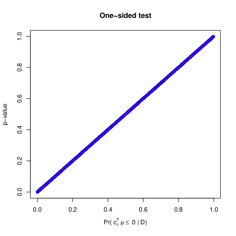
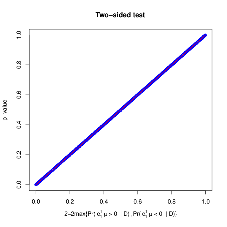
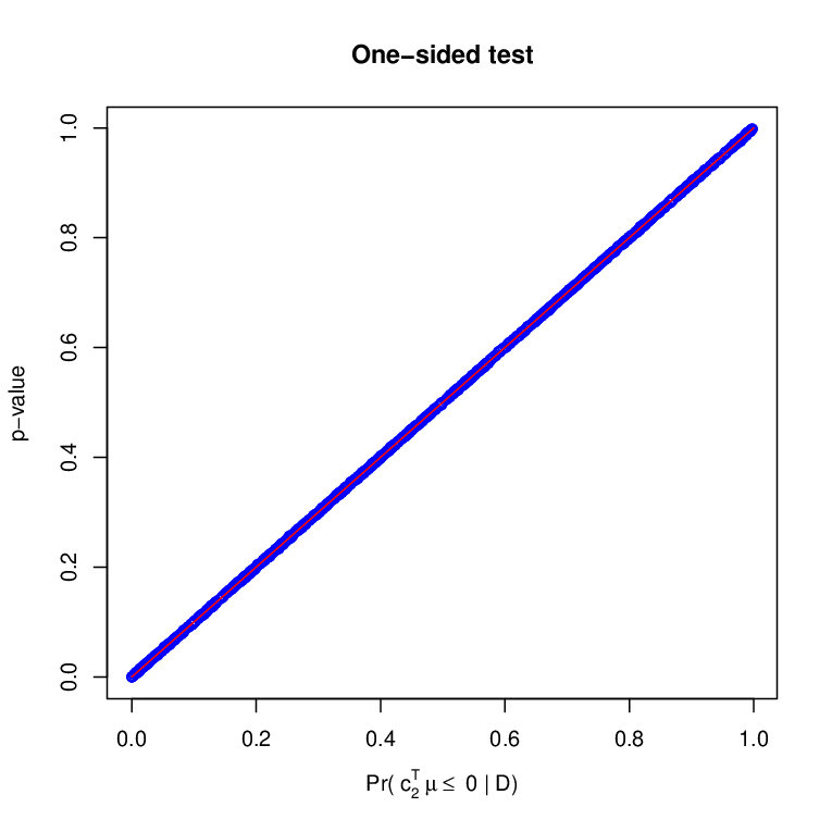
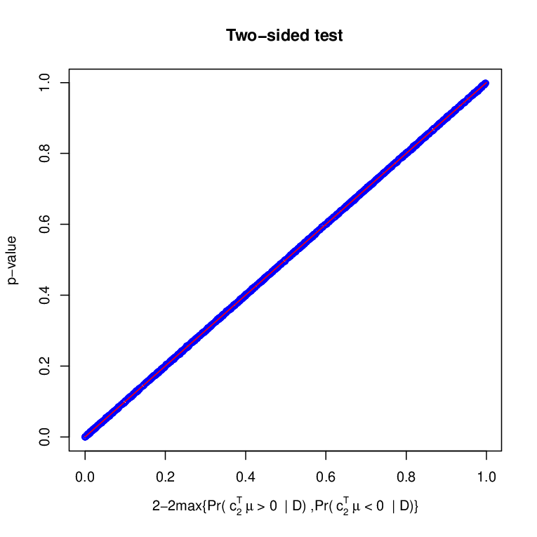
For illustration, we conduct a numerical study to compute the posterior probabilities of for , and compare them with the corresponding -values. We take and to be a unit vector with 1 on the th element and 0 otherwise, and assume a vague normal prior distribution for , i.e., and , where is a -dimensional identity matrix. The relationship between the posterior probabilities of the null and -values is shown in Figure 4, which again demonstrates their equivalence for both one-sided and two-sided tests.
6 Random Effects Models
We further consider a random effects model and conduct hypothesis testing for both regression coefficients and variance components. The data are generated from a linear random effects model as follows,
where is the outcome of observation in cluster , ; and covariates ’s are generated from . We assume and . The sample size is , and the cluster size is , and we set the true parameter values to be , and in our numerical study.
We consider a one-sided test for ,
and another one-sided test for ,
We vary the values of and , and for each configuration we use the Wald test to obtain the -value and compare it with the posterior probability (PoP) of the null hypothesis. For the frequentist test on , we use the asymptotic distribution based on the Fisher information,
and by the delta method, we take the log transformation,
Figure 5 shows that for different values of and the -values and the posterior probabilities of the null hypothesis are very close, especially under the settings of . The match between the two quantities appear to be better for the tests of the regression coefficient than those of the variance component.
7 Discussion
The -value is the most commonly used summary measure for evidence-based studies, and it has been the center of controversies and debates for decades. Recently reignited discussion over -values has been more centered around the proposals to adjust, abandon or provide alternatives to -values. By definition, -value is not the probability that the null hypothesis is true given the observed data. Contrary to the conventional notion, it does have a close correspondence to the Bayesian posterior probability of the null hypothesis being true for both one-sided and two-sided hypothesis tests. Certainly, such equivalence relationship would not hold when informative priors are used, because -values are computed without any prior information involved. Lindley’s paradox mainly arises when a point mass is put on the parameter of interest under the null hypothesis. We circumvent the controversy by recasting a two-sided hypothesis into two one-sided hypotheses, and then the paradox can be explained: the -value and the Bayesian posterior probability of the null hypothesis coincide.
References
-
Bayarri, M. J. and Berger, J. O. (2004). The interplay of Bayesian and frequentist analysis. Statistical Science 19, 58–80.
-
Benjamin, D. J. and Berger J. O. (2019). Three recommendations for improving the use of p-values. The American Statistician 73, 186–191.
-
Berger, J. O. (2003). Could Fisher, Jeffreys and Neyman have agreed on testing? (with discussion) Statistical Science 18, 1–32.
-
Berger, J. O. and Delampady M. (1987). Testing precise hypotheses. Statistical Science 2, 317–335.
-
Berger, J. O. and Sellke, T. (1987). Testing a point null hypothesis: the irreconcilability of P values and evidence. Journal of the American Statistical Association 82, 112–122.
-
Betensky, R. A. (2019). The p-value requires context, not a threshold. The American Statistician 73, 115–117.
-
Billheimer, D. (2019). Predictive inference and scientific reproducibility. The American Statistician 73, 291–295.
-
Casella, G. and Berger, R. L. (1987). Reconciling Bayesian and frequentist evidence in the one-sided testing problem. (with discussion) Journal of the American Statistical Association 82, 106–111.
-
Colquhoun, D. (2019). The false positive risk: a proposal concerning what to do about p-values. The American Statistician 73, 192–201.
-
Gannon, M. A., Pereira, C. A. B., Polpo, A. (2019). Blending Bayesian and classical tools to define optimal sample-size-dependent significance levels. The American Statistician 73, 213–222.
-
Goodman, S. N. (1999). Toward evidence-based medical statistics. 1: the p value fallacy. Annals of Internal Medicine 130, 995–1004.
-
Hubbard, R. and Lindsay, R. M. (2008). Why P values are not a useful measure of evidence in statistical significance testing. Theory Psychology 18: 69–88.
-
Ioannidis, J. P. (2019). What have we (not) learnt from millions of scientific papers with p values? The American Statistician 73, 20–25.
-
Johnson, V. E. and Rossell, D. (2010). On the use of non-local prior densities in Bayesian hypothesis tests. Journal of the Royal Statistical Society: Series B (Statistical Methodology) 72, 143–170.
-
Johnson, V. E. (2019). Evidence from marginally significant t statistics. The American Statistician 73, 129–134.
-
Kennedy-Shaffer, L. (2019). Before p to beyond p : using history to contextualize p-values and significance testing. The American Statistician 73, 82–90.
-
Krueger, J. I. and Heck, P. R. (2019). Putting the p-value in its place. The American Statistician 73, 122–128.
-
Lindley, D. V. (1957). A statistical paradox. Biometrika 44, 187–192.
-
Manski, C. F. (2019). Treatment choice with trial data: statistical decision theory should supplant hypothesis testing. The American Statistician 73, 296–304.
-
Matthews, R. A. J. (2019). Moving towards the post p era via the analysis of credibility. The American Statistician 73, 202–212.
-
McShane, B. B., Gal, D., Gelman, A., Robert, C., and Tackett, J. L. (2019). Abandon statistical significance. The American Statistician 73, 235–245.
-
Pratt, J. W. (1965). Bayesian interpretation of standard inference statements (with discussion). Journal of the Royal Statistical Society, Series B 27, 169–203.
-
Rougier, J. (2019). p-values, Bayes factors, and sufficiency. The American Statistician 73, 148–151.
-
Ruberg, S. J., Harrell Jr., F. E., Gamalo-Siebers, M., LaVange, L., Lee, J. J., Price, K., Peck, C. (2019). Inference and decision making for 21st-century drug development and approval. The American Statistician 73, 319–327.
-
Sellke, T., Bayarri, M. J., and Berger, J. O. (2001). Calibration of p-values for testing precise null hypotheses. The American Statistician 55, 62–71.
-
Shi, H. and Yin, G. (2020). Reconnecting p-value and posterior probability under one- and two-sided tests. The American Statistician DOI: 10.1080/00031305.2020.1717621
-
Wagenmakers, E. J. (2007). A practical solution to the pervasive problems of p-values. Psychonomic Bulletin Review 14, 779–804.
-
Wasserstein, R. L. and Lazar, N. A. (2016). The ASA’s statement on p-values: context, process, and purpose. The American Statistician 70, 129–133.
-
Wasserstein, R. L., Schirm, A. L., and Lazar, N. A. (2019). Moving to a world beyond “p”. The American Statistician 73, 1–19.
| 1 | 0.01793728 |
|---|---|
| 0.1 | 0.01793580 |
| 0.01 | 0.01793565 |
| 0.001 | 0.01793564 |
| 0.0001 | 0.01793563 |
| 0.00001 | 0.01793563 |
| 0.000001 | 0.01793563 |
| 2 | 0.059235 |
|---|---|
| 1.5 | 0.052752 |
| 1 | 0.046143 |
| 0.9 | 0.044809 |
| 0.8 | 0.043471 |
| 0.7 | 0.042131 |
| 0.6 | 0.040789 |
| 0.5 | 0.039445 |
| 0.4 | 0.038099 |
| 0.3 | 0.036753 |
| 0.2 | 0.035406 |
| 0.1 | 0.034060 |
| 0.01 | 0.032849 |
| 0.001 | 0.032728 |
| 0.0001 | 0.032716 |
| 0.00001 | 0.032715 |
| 0.000001 | 0.032715 |