Energy transport between critical one-dimensional systems
with different central charges

Transport properties are one of the most fundamental ways to characterise and classify condensed matter systems. Electrical transport properties, for instance, can distinguish metals from insulators or superconductors. Very specific electrical transport properties can further fan out the classification, for example, insulating bulk systems can have interesting boundary transport properties, as is the case in quantum Hall systems, topological insulators, or other topologically ordered systems.

Although generally more complicated to measure and compute, the same is true for heat transport. Additional difficulties arise in this case from the fact that all degrees of freedom participate in the transport process and not only those associated with a charge under the electromagnetic field, ie, phonons and collective modes also contribute. In the early days of research on metals it was established that to an excellent degree of approximation those systems fulfilled the so-called Wiedemann–Franz law.WiedemannFranz53 This law states that as the temperature $T$ goes to zero, the ratio of the electrical conductivity $\sigma$ and the heat conductivity $\kappa$ tends to $\sigma/\kappa=TL_{0}$ where $L_{0}=\pi^{2}k_{\text{B}}^{2}/(3e^{2})$ is the Lorenz number, a constant only composed out of fundamental quantities. Nowadays, the Wiedemann–Franz law or the violation thereofWakeham-11; Crossno-16; Dutta-17 serves as a diagnostic tool for the existence or non-existence of a Fermi liquid state.

In one-dimensional systems, more recent workBernardDoyon12 uncovered a fundamental connection between the central charge of a critical system with conformal symmetry and its heat-transport properties. If the system is characterised by a central charge $c$, but it consists of two subsystems, left and right, held at temperatures $T_{\text{L}}$ and $T_{\text{R}}$ respectively, the energy current is given by

$\displaystyle J_{\text{E}}=\frac{c\pi}{12}\left(T_{\text{L}}^{2}-T_{\text{R}}^{2}\right),$

(1)

and thus directly proportional to the central charge itself. The central charge can be interpreted loosely as a measure for the number of degrees of freedom in a theory. It describes how a system behaves in the presence of a macroscopic length scale, for example the Casimir energy is directly proportional to $c$. At a more formal level, the central charge dictates the short-distance behaviour of the correlation functions of the energy-momentum tensor and appears as a quantum anomaly.DiFrancescoMathieuSenechal97; Mussardo10 It is important to note that for the result (1) to hold, overall translational invariance of the equilibrium situation $T_{\text{L}}=T_{\text{R}}$ is required. The result (1) was subsequently confirmed in free systems like the transverse-field Ising chainDeLuca-13; ColluraKarevski14; Kormos17; PerfettoGambassi17 as well as interacting systems using the generalised hydrodynamic approachCastro-Alvaredo-16; Bertini-16; BertiniPiroli18; Horvath19 and numerical simulations.Karrasch-13; DeLuca-14; Biella-16

The purpose of this paper is two-fold: we first verify the result (1) for two microscopic models corresponding to field theories with $c=1$ and $c=1/2$, ie, free fermions and free Majorana fermions, respectively. Additionally, we study a situation in which we couple two subsystems with these two different central charges. As our main result we find a bottleneck on the energy current, namely the subsystem with the smaller central charge limits the energy transport. The convenient framework to study this is a one-dimensional version of a spinless p-wave superconductor, which can realise central charges of $c=1$ and $c=1/2$ at its respective XX and Ising critical point. We will use two complementary methods: (i) the non-equilibrium Green function technique,RammerSmith86; Kamenev11 which allows us to obtain exact analytical results in the thermodynamic limit at all parameter regimes, and (ii) the real-timeVidal04; WhiteFeiguin04; Daley-04; Schmitteckert04 finite-temperatureFeiguinWhite05; Barthel-09 density matrix renormalisation group (DMRG)White92; Schollwoeck11 algorithmKarrasch-12; Karrasch-13NJP; Karrasch-13 which works directly with the corresponding lattice models.

The organisation of the paper is as follows: we first introduce the model in Sec. II and briefly review its key properties. Sec. III discusses the basic the energy current operator in its most generic form and relates it to Green functions, while Sec. IV gives details on the DMRG simulations. In Sec. V we present our main results and finish with a conclusion in Sec. VI. Technical details are deferred to the appendices.

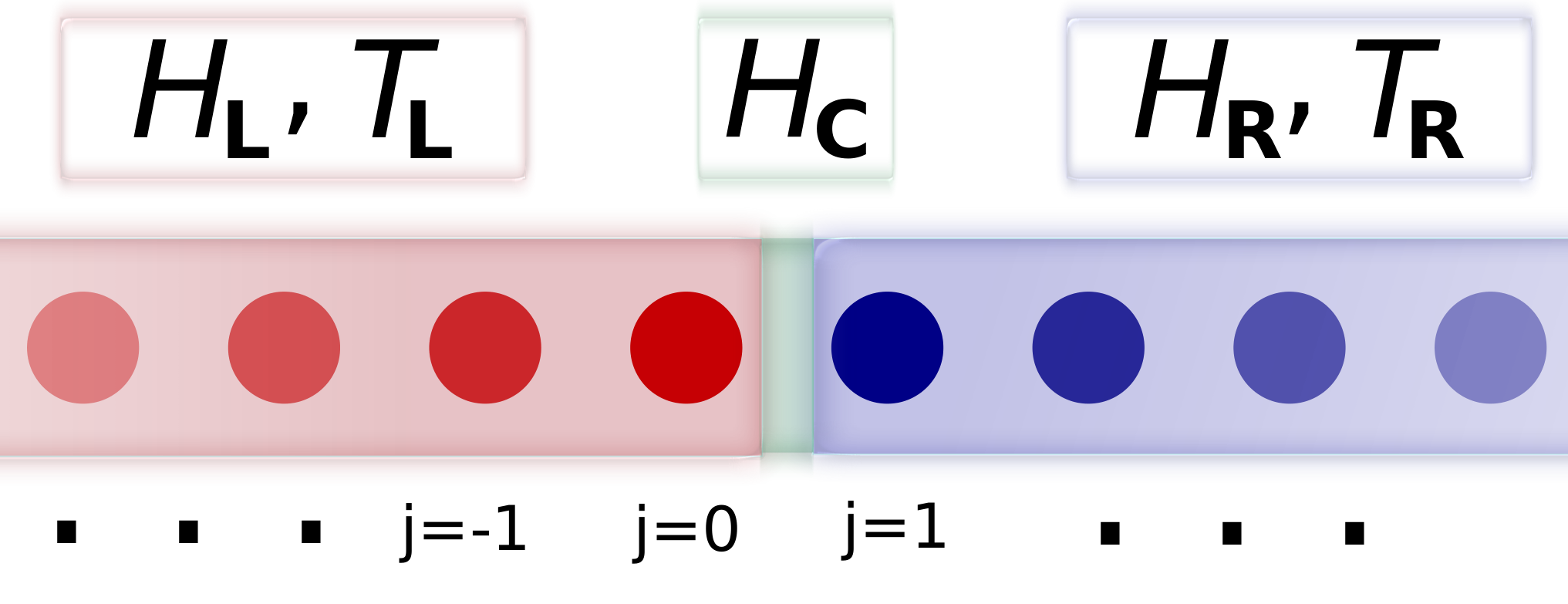
The setup we consider consists of two subsystems, henceforth referred to as ‘left’ (L) and ‘right’ (R). Both are held at different but constant temperatures $T_{\text{L}}$ and $T_{\text{R}}$ and are described by Hamiltonians $H_{\text{L}}$ and $H_{\text{R}}$, respectively. The two subsystems are coupled by a Hamiltonian $H_{\text{C}}$ which facilitates energy flow between them, see Fig. 1 for a sketch of the setup. Specifically we consider a Hamiltonian of the type

	$\displaystyle H$	$\displaystyle=$	$\displaystyle H_{\text{L}}+H_{\text{R}}+H_{\text{C}},$		(2)
	$\displaystyle H_{\text{L}}$	$\displaystyle=$	$\displaystyle-t_{\text{L}}\sum_{j=-N_{\text{L}}}^{-1}\left(c_{j}^{\dagger}c_{j+1}^{\phantom{\dagger}}+c_{j+1}^{\dagger}c_{j}^{\phantom{\dagger}}\right)-\epsilon_{\text{L}}\sum_{j=-N_{\text{L}}}^{0}c^{\dagger}_{j}c^{\phantom{\dagger}}_{j}$		(3)
			$\displaystyle-\Delta_{\text{L}}\sum_{j=-N_{\text{L}}}^{-1}\left(c_{j}^{\dagger}c_{j+1}^{\dagger}+c_{j+1}^{\phantom{\dagger}}c_{j}^{\phantom{\dagger}}\right),$
	$\displaystyle H_{\text{R}}$	$\displaystyle=$	$\displaystyle-t_{\text{R}}\sum_{j=1}^{N_{\text{R}}-1}\left(c_{j}^{\dagger}c_{j+1}^{\phantom{\dagger}}+c_{j+1}^{\dagger}c_{j}^{\phantom{\dagger}}\right)-\epsilon_{\text{R}}\sum_{j=1}^{N_{\text{R}}}c^{\dagger}_{j}c^{\phantom{\dagger}}_{j}$		(4)
			$\displaystyle-\Delta_{\text{R}}\sum_{j=1}^{N_{\text{R}}-1}\left(c_{j}^{\dagger}c_{j+1}^{\dagger}+c_{j+1}^{\phantom{\dagger}}c_{j}^{\phantom{\dagger}}\right),$
	$\displaystyle H_{\text{C}}$	$\displaystyle=$	$\displaystyle-t_{\text{C}}\left(c_{0}^{\dagger}c_{1}^{\phantom{\dagger}}+c_{1}^{\dagger}c_{0}^{\phantom{\dagger}}\right)-\Delta_{\text{C}}\left(c_{0}^{\dagger}c_{1}^{\dagger}+c_{1}^{\phantom{\dagger}}c_{0}^{\phantom{\dagger}}\right).$		(5)

This Hamiltonian describes a one-dimensional p-wave superconductor with hopping parameters $t_{\text{L}},t_{\text{R}},t_{\text{C}}$ and pairing terms $\Delta_{\text{L}},\Delta_{\text{R}},\Delta_{\text{C}}$ in their respective parts of the chain. The operator $c_{j}$ is an annihilation operator for a spinless fermion at site $j$ where negative (positive) $j$ indicate a site in the left (right) subsystem (site $0$ belongs to the left subsystem). We note that the total number of lattice sites equals $N_{\text{L}}+N_{\text{R}}+1$. Additionally, we introduce on-site energies $\epsilon_{\text{L}}$ and $\epsilon_{\text{R}}$.

The main motivation to study this Hamiltonian is that it allows for a variety of different situations including that of having different central charges $c_{\text{L,R}}=1/2,1$ in the respective subsystems, as well as different speeds of light. For example, the $c_{\text{L}}=1/2$ critical point is obtained for $t_{\text{L}}=\Delta_{\text{L}}=\epsilon_{\text{L}}/2$, with the velocity of the low-lying excitations given by $v=2t_{\text{L}}$. On the other hand, $c_{\text{L}}=1$ is obtained for the choice $\Delta_{\text{L}}=\epsilon_{\text{L}}=0$ with the velocity $v=2t_{\text{L}}$. For most other parameter sets this Hamiltonian describes a gapped system which one can also study, as done in Sec. V.1. These situations, however, are of little interest to our discussion since at this point a comparison to the result Eq. (1) is impossible. If one is looking into experimental situations, this type of Hamiltonian can be encountered in a variety of settings. Apart from direct electronic implementations it can also appear as an effective model of spin chains via a Jordan–Wigner transformationGiamarchi04 (see Appendix A).

The heat current is the temporal change of heat in either of the two subsystems. It consists of two contributions, namely a change in the energy and one related to the particle flow. Choosing the left lead as reference, it is given byGiazotto-06 $Q_{\text{L}}=J_{\text{E}}-\mu\dot{N}_{\text{L}}$ where $Q_{\text{L}}$ is the heat flowing out of the left lead, while $J_{\text{E}}=-\dot{E}_{\text{L}}$ and $-\dot{N}_{\text{L}}$ are the energy and particle flows, respectively, and $\mu$ denotes an external chemical potential. In the remainder of this work we only consider the case $\mu=0$ implying the heat current is equal to the temporal change of energy in the lead, ie, $Q_{\text{L}}=J_{\text{E}}=-\dot{E}_{\text{L}}$. Furthermore, we are only interested in the steady state heat current where we have $Q_{\text{L}}=-Q_{\text{R}}$.

In order to derive the energy current in the left lead we use the Heisenberg equations of motion following $\dot{E}_{\text{L}}=\frac{\text{d}}{\text{d}t}\langle H_{\text{L}}\rangle=\text{i}\langle[H,H_{\text{L}}]\rangle$ (note that $\hbar=1$ throughout). Straightforward computations allow to rewrite this in terms of the fermionic operators as

	$\displaystyle\dot{E}_{\text{L}}$	$\displaystyle=$	$\displaystyle-\text{i}\left(t_{\text{L}}t_{\text{C}}-\Delta_{\text{L}}\Delta_{\text{C}}\right)\left\langle c^{\dagger}_{-1}c^{\phantom{\dagger}}_{1}+c^{\phantom{\dagger}}_{-1}c^{\dagger}_{1}\right\rangle$		(6)
			$\displaystyle-\text{i}\left(t_{\text{L}}\Delta_{\text{C}}-t_{\text{C}}\Delta_{\text{L}}\right)\left\langle c_{-1}^{\phantom{\dagger}}c_{1}^{\phantom{\dagger}}+c_{-1}^{\dagger}c_{1}^{\dagger}\right\rangle$
			$\displaystyle-\text{i}t_{\text{C}}\epsilon_{\text{L}}\left\langle c_{0}^{\phantom{\dagger}}c_{1}^{\dagger}+c_{0}^{\dagger}c_{1}^{\phantom{\dagger}}\right\rangle-\text{i}\Delta_{\text{C}}\epsilon_{\text{L}}\left\langle c_{0}^{\phantom{\dagger}}c_{1}^{\phantom{\dagger}}+c_{0}^{\dagger}c_{1}^{\dagger}\right\rangle.\quad$

It is important to note here that apart from ‘normal’ fermionic Green functions this also requires knowledge of anomalous propagators due to the superconducting correlations. The calculations are carried out in a non-equilibrium setting and we consequently resort to the Schwinger–Keldysh closed time contour formalism,Kamenev11 which we use to derive exact results in the thermodynamic limit. We note that this requires the system to be an effectively free theory, in our case corresponding to $c=1/2$ and $c=1$ respectively. In contrast, the application of the non-equilibrium Green function technique to interacting theories would require approximations. Using the results and definitions from Appendix B [especially Eq. (59)–(62)] the above expectation values can be expressed in terms of lesser Green functions according to

	$\displaystyle\dot{E}_{\text{L}}$	$\displaystyle=$	$\displaystyle\phantom{+}\left(t_{\text{L}}t_{\text{C}}-\Delta_{\text{L}}\Delta_{\text{C}}\right)\text{Re}\left[G^{<}_{1,-1}(t,t)+\bar{G}^{<}_{1,-1}(t,t)\right]$		(7)
			$\displaystyle+\left(t_{\text{L}}\Delta_{\text{C}}-\Delta_{\text{L}}t_{\text{C}}\right)\text{Re}\left[F^{<}_{1,-1}(t,t)+\bar{F}^{<}_{1,-1}(t,t)\right]$
			$\displaystyle+t_{\text{C}}\epsilon_{\text{L}}\text{Re}\left[G^{<}_{1,0}(t,t)+\bar{G}^{<}_{1,0}(t,t)\right]$
			$\displaystyle+\Delta_{\text{C}}\epsilon_{\text{L}}\text{Re}\left[F^{<}_{1,0}(t,t)+\bar{F}^{<}_{1,0}(t,t)\right],$

where $G^{<}$ and $\bar{G}^{<}$ denote the normal particle and hole propagators and $F^{<}$ and $\bar{F}^{<}$ describe anomalous propagators for Cooper pairs and anti-Cooper pairs respectively [see Eq. (9) below]. Restricting ourselves to a steady state situation allows to apply Fourier transformation from time into frequency domain. Furthermore, we can significantly simplify the expression for the current using the Dyson equation for the lesser Green functions.

Since lesser Green functions are off-diagonal in terms of the time contour description, the Dyson equation for the lesser Green function reads

$$\sum_{j}\hat{G}^{<}_{i,j}\left(\omega\,\delta_{j,k}-\mathcal{H}_{j,k}\right)=0,$$

(8)

where the Green function $\hat{G}$ is a matrix in Nambu space that has the structure

$$\hat{G}_{j,k}(\omega)=\begin{pmatrix}G&F\\ \bar{F}&\bar{G}\end{pmatrix}_{j,k}(\omega)$$

(9)

and $\mathcal{H}_{j,k}$ denotes the matrix representation of the Hamiltonian; see Eq. (51) for the precise form. Using Eq. (8) in the case of $i=1$ and $k=0$, we can rewrite the energy current in a compact form as

$$\begin{split}\dot{E}_{\text{L}}=&-\int\frac{\text{d}\omega}{2\pi}\text{Re}\left\{\omega\left[t_{\text{C}}\left(G-\bar{G}\right)_{1,0}-\Delta_{\text{C}}\left(F-\bar{F}\right)_{1,0}\right]^{<}\right.\\ &\left.\!\!\!\!+\left[\left(t_{\text{C}}^{2}-\Delta_{\text{C}}^{2}\right)\left(G+\bar{G}\right)_{1,1}+2t_{\text{C}}\Delta_{\text{C}}\left(F+\bar{F}\right)_{1,1}\right]^{<}\right\}.\end{split}$$

(10)

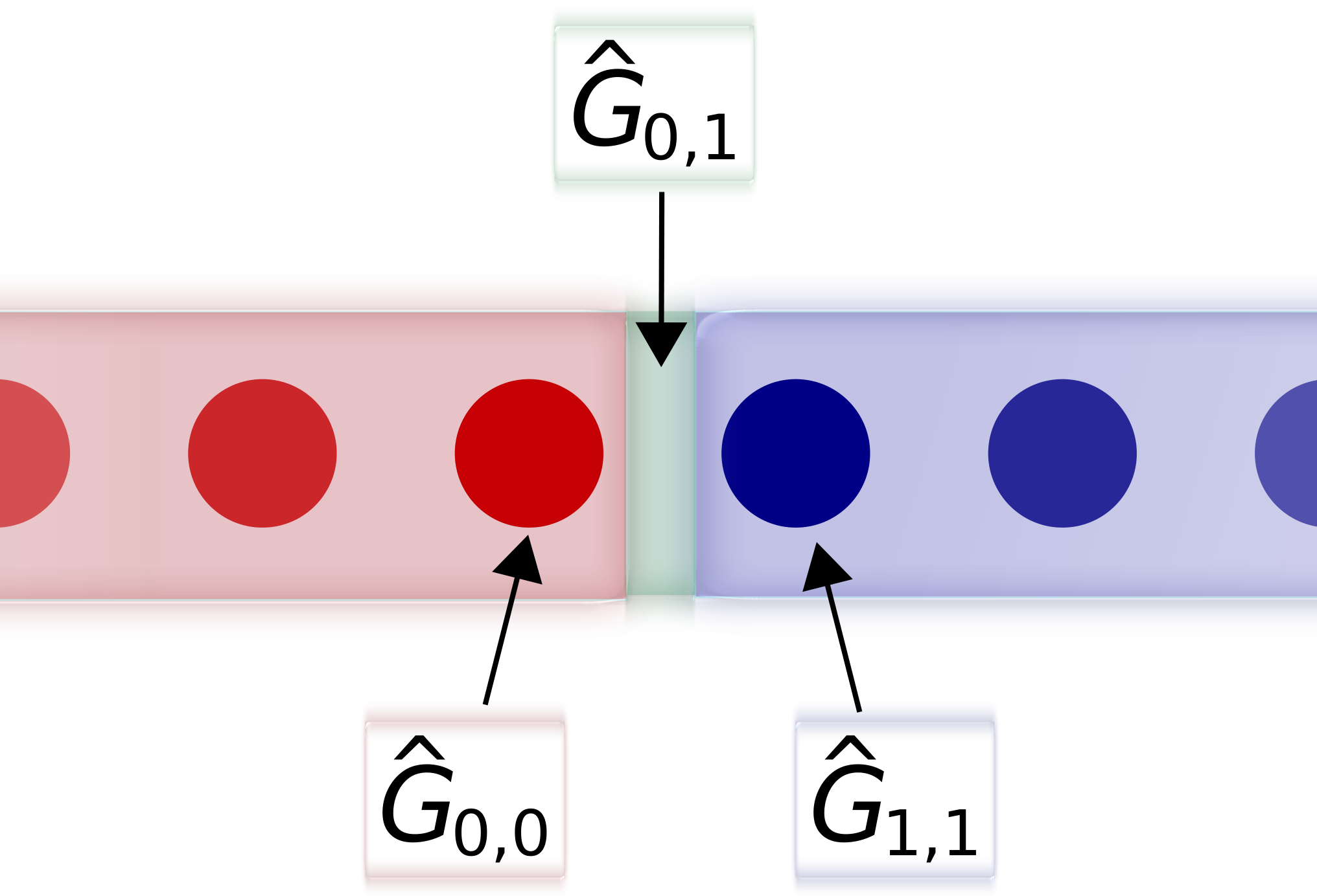
Unless specified the integration ranges over the real axis, $-\infty<\omega<\infty$. Also from now on the Green functions are understood to depend on the frequency $\omega$. The second line of Eq. (10) does not contribute since the local lesser Green functions do not have a real part and thus we can drop them. Importantly, this expression depends solely on the Green function that describes the transition from the last side of the left lead to the first side of the right lead, whereas the rest of the system does not contribute explicitly. Furthermore, using the results of Appendix C, we can decompose this element of the Green function into two parts that only contain local Green functions situated at the ends of each lead according to

$$\hat{G}_{1,0}=-\hat{G}^{(0)}_{1,1}\,\hat{t}_{\text{C}}\,\hat{G}_{0,0},$$

(11)

which is graphically represented in Fig. 2. Specifically, the transition Green function consists of one bare Green function $\hat{G}^{(0)}_{1,1}$, one full Green function $\hat{G}_{0,0}$, and a coupling matrix $\hat{t}_{\text{C}}$ that is given by

$$\hat{t}_{\text{C}}=\begin{pmatrix}t_{\text{C}}&\Delta_{\text{C}}\\ -\Delta_{\text{C}}&-t_{\text{C}}\end{pmatrix}.$$

(12)

In this context the bare Green function $\hat{G}^{(0)}_{1,1}$ is the Green function of the first site of the right chain with the left chain decoupled, whereas the full Green function $\hat{G}_{0,0}$ is the one of the last site of the left lead computed in the presence of a coupling to the right lead. It is worthwhile noting that the choice of ’bare’ for the right lead and ’full’ for the left lead is arbitrary and could be switched around.

Although it is possible to perform all the calculations for the full model (2), for the sake of brevity we specify below to the relevant cases possessing conformal symmetry.

In order to compute the energy current $J_{\textnormal{E}}$ using the DMRG method,White92; Schollwoeck11 we consider the setup shown in Fig. 1 as an initial condition and subsequently perform a time-evolution until a stationary state is reached. In practice, one can reach only finite time scales (see below), which are typically of the order of several $\mathcal{O}(10/t_{\textnormal{L,R}})$. This leads to a finite-time error whose magnitude one can estimate, eg, by interchanging $T_{\textnormal{L}}\leftrightarrow T_{\textnormal{R}}$ and comparing results (which agree only in the limit $t\to\infty$).

To be more precise, the thermal density matrices $e^{-H_{\textnormal{L,R}}/T}$ as well as the real-time evolution operators $e^{-iHt}$ are determined using a time-dependent DMRG algorithm; both operators are factorized by a fourth order Trotter-Suzuki decomposition.Vidal04; WhiteFeiguin04; Daley-04; Schmitteckert04 We incorporate finite temperatures using the purification technique.FeiguinWhite05; Barthel-09 The discarded weight during each individual ‘bond update’ is kept below a pre-defined discarded weight, which leads to an exponential increase of the bond dimension during the real-time evolution. In order to access time scales as large as possible, we employ a finite-temperature disentangler, Karrasch-12; Karrasch-13NJP which exploits the fact that purification is not unique to slow down the growth of the bond dimension. Our calculations are performed using a system size of the order of $N_{\textnormal{L}}=N_{\textnormal{R}}=128$ sites. The Hamiltonian is transformed into a spin representation via a Jordan-Wigner transformation (see Appendix A).

In the following we discuss three different cases: (a) Coupling two subsystems with effective Majorana degrees of freedom, ie, $c=1/2$ in both subsystems. (b) Coupling two free fermion systems, ie, $c=1$ in both subsystems. (c) Coupling a Majorana fermion to a fermion system, meaning $c=1/2$ and $c=1$ in the respective subsystems. We note that while the first two cases realise a setup covered by Eq. (1) at their respective massless points, provided there is overall translational symmetry of the parameters of the Hamiltonian, in the latter situation the result Eq. (1) is not applicable. Furthermore, we simplify the setup by always choosing the parameters of the coupling region, described by Eq. (5), to equal the parameters of the right lead, ie, $t_{\text{C}}=t_{\text{R}}$ and $\Delta_{\text{C}}=\Delta_{\text{R}}$.

In this work we studied the energy transport in one-dimensional critical systems which are characterised by differing central charges. The model we studied was a p-wave superconductor which allows to realise two different conformal field theories in its low-energy limit: a theory of free fermions corresponding to central charge $c=1$ and free Majorana fermions corresponding to $c=1/2$. In translationally invariant systems we verified, using an exact non-equilibrium Green function calculation as well as DMRG simulations, that the low-energy limit of the energy current is indeed given by Eq. (1).

Going beyond this we considered systems consisting of two different semi-infinite chains realising a $c=1$ and $c=1/2$ conformal field theory. Since translation invariance is broken in this setup, the result (1) is not applicable. Nevertheless, our result (40) for the maximal energy current has the same functional form with the central charge of the Majorana system limiting the energy current. One can interpret our result in the sense that the subsystem possessing the smaller central charge and thus the fewer degrees of freedom limits the energy transport, in the same way that the number of open transport channels limits charge currents in the Landauer–Büttiker formalism. In such a picture the limited number of degrees of freedom in the Majorana system thus serves as a bottleneck for the transport through the junction. With this interpretation in mind we conjecture that the maximal energy current between two critical systems possessing central charges $c_{\text{L}}$ and $c_{\text{R}}$ should have the form

$$J_{\text{E}}=\frac{\pi}{12}\,\min(c_{\text{L}},c_{\text{R}})\,(T_{\text{L}}^{2}-T_{\text{R}}^{2}).$$

(41)

For the future it would be interesting to verify that this bottleneck effect also shows up in interacting systems like the XXZ Heisenberg chain and systems corresponding to conformal field theories with central charge $c\neq 1$. An example for the latter setup would be provided by coupling a critical three-state Potts chain to Majorana fermions.

We thank Denis Bernard, Axel Cortés Cubero, Benjamin Doyon, Michael Wimmer, Jacopo Viti and particularly Tatjana Puškarov for useful discussions. DS would like to thank the organisers of the 2016 programme “Mathematical aspects of quantum integrable models in and out of equilibrium” at the Isaac Newton Institute for Mathematical Sciences, where this work was partially inspired. This work is part of the D-ITP consortium, a program of the Netherlands Organisation for Scientific Research (NWO) that is funded by the Dutch Ministry of Education, Culture and Science (OCW). CK acknowledges support by the Deutsche Forschungsgemeinschaft through the Emmy Noether program (KA 3360/2-1).

References

- (1) G. Wiedemann and R. Franz, Ueber die Wärme-Leitungsfähigkeit der Metalle, Annalen der Physik und Chemie 89, 32 (1853).
- (2) N. Wakeham, A. F. Bangura, X. Xu, J.-F. Mercure, M. Greenblatt and N. E. Hussey, Gross violation of the Wiedemann-Franz law in a quasi-one-dimensional conductor, Nature Commun. 2, 396 (2011).
- (3) J. Crossno, J. K. Shi, K. Wang, X. Liu, A. Harzheim, A. Lucas, S. Sachdev, P. Kim, T. Taniguchi, K. Watanabe, T. A. Ohki and K. C. Fong, Observation of the Dirac fluid and the breakdown of the Wiedemann-Franz law in graphene, Science 351, 1058 (2016).
- (4) B. Dutta, J. T. Peltonen, D. S. Antonenko, M. Meschke, M. A. Skvortsov, B. Kubala, J. König, C. B. Winkelmann, H. Coutois and J. P. Pekola, Thermal conductance of a single-electron transistor, Phys. Rev. Lett. 119, 077701 (2017).
- (5) D. Bernard and B. Doyon, Energy flow in non-equilibrium conformal field theory, J. Phys. A 45, 362001 (2012).
- (6) P. Di Francesco, P. Mathieu and D. Sénéchal, Conformal Field Theory (Springer, New York, 1997).
- (7) G. Mussardo, Statistical Field Theory (Oxford University Press, Oxford, 2010).
- (8) A. De Luca, J. Viti, D. Bernard and B. Doyon, Nonequilibrium thermal transport in the quantum Ising chain, Phys. Rev. B 88, 134301 (2013).
- (9) M. Collura and D. Karevski, Quantum quench from a thermal tensor state: Boundary effects and generalized Gibbs ensemble, Phys. Rev. B 89, 214308 (2014).
- (10) M. Kormos, Inhomogeneous quenches in the transverse field Ising chain: scaling and front dynamics, SciPost Phys. 3, 020 (2017).
- (11) G. Perfetto and A. Gambassi, Ballistic front dynamics after joining two semi-infinite quantum Ising chains, Phys. Rev. E 96, 012138 (2017).
- (12) O. A. Castro-Alvaredo, B. Doyon and T. Yoshimura, Emergent hydrodynamics in integrable quantum systems out of equilibrium, Phys. Rev. X 6, 041065 (2016).
- (13) B. Bertini, M. Collura, J. De Nardis and M. Fagotti, Transport in out-of-equilibrium chains: Exact profiles of charges and currents, Phys. Rev. Lett. 117, 207201 (2016).
- (14) B. Bertini and L. Piroli, Low-temperature transport in out-of-equilibrium XXZ chains, j. Stat. Mech. (2018) 033104.
- (15) D. X. Horváth, Hydrodynamics of massless integrable RG flows and a non-equilibrium c-theorem, J. High Energy Phys. 2019, 20 (2019).
- (16) C. Karrasch, R. Ilan and J. E. Moore, Nonequilibrium thermal transport and its relation to linear response, Phys. Rev. B 88, 195129 (2013).
- (17) A. De Luca, J. Viti, L. Mazza and D. Rossini, Energy transport in Heisenberg chains beyond the Luttinger liquid paradigm, Phys. Rev. B 90, 161101 (2014).
- (18) A. Biella, A. De Luca, J. Viti, D. Rossini, L. Mazza and R. Fazio, Energy transport between two integrable spin chains, Phys. Rev. B 93, 205121 (2016).
- (19) J. Rammer and H. Smith, Quantum field-theoretical methods in transport theory of metals, Rev. Mod. Phys. 58, 323 (1986).
- (20) A. Kamenev, Field theory of non-equilibrium systems (Cambridge University Press, Cambridge, 2011).
- (21) G. Vidal, Efficient simulation of one-dimensional quantum many-body systems, Phys. Rev. Lett. 93, 040502 (2004).
- (22) S. R. White and A. E. Feiguin, Real-time evolution using the density matrix renormalization group, Phys. Rev. Lett. 93, 076401 (2004).
- (23) A. J. Daley, C. Kollath, U. Schollwöck and G. Vidal, Time-dependent density-matrix renormalization-group using adaptive effective Hilbert spaces, J. Stat. Mech. P04005 (2004).
- (24) P. Schmitteckert, Nonequilibrium electron transport using the density matrix renormalization group method, Phys. Rev. B 70, 121302(R) (2004).
- (25) A. E. Feiguin and S. R. White, Finite-temperature density matrix renormalization using an enlarged hilbert space, Phys. Rev. B 72, 220401 (2005).
- (26) T. Barthel, U. Schollwöck and S. R. White, Spectral functions in one-dimensional quantum systems at finite temperature using the density matrix renormalization group, Phys. Rev. B 79, 245101 (2009).
- (27) S. R. White, Density Matrix Formulation for Quantum Renormalization Groups, Phys. Rev. Lett. 69, 2863 (1992).
- (28) U. Schollwöck, The density-matrix renormalization group in the age of matrix product states, Ann. Phys. 326, 96 (2011).
- (29) C. Karrasch, J. H. Bardarson and J. E. Moore, Finite-temperature dynamical density matrix renormalization group and the drude weight of spin- chains, Phys. Rev. Lett. 108, 227206 (2012).
- (30) —, Reducing the numerical effort of finite-temperature density matrix renormalization group calculations, New J. Phys. 15, 083031 (2013).
- (31) T. Giamarchi, Quantum Physics in One Dimension (Oxford University Press, Oxford, 2004).
- (32) F. Giazotto, T. T. Heikkilä, A. Luukanen, A. M. Savin and J. P. Pekola, Opportunities for mesoscopics in thermometry and refrigeration: Physics and applications, Rev. Mod. Phys. 78, 217 (2006).
- (33) H. Haug and A.-P. Jauho, Quantum Kinetics in transport and optics of semiconductors (Springer, Berlin, 2008).
- (34) D. Bernard, B. Doyon and J. Viti, Non-equilibrium conformal field theories with impurities, J. Phys. A 48, 05FT01 (2015).
- (35) L. Mazza, J. Viti, M. Carrega, D. Rossini and A. De Luca, Energy transport in an integrable parafermionic chain via generalized hydrodynamics, Phys. Rev. B 98, 075421 (2018).