Operational definition of a quantum speed limit
Abstract
The quantum speed limit is a fundamental concept in quantum mechanics, which aims at finding the minimum time scale or the maximum dynamical speed for some fixed targets. In a large number of studies in this field, the construction of valid bounds for the evolution time is always the core mission, yet the physics behind it and some fundamental questions like which states can really fulfill the target, are ignored. Understanding the physics behind the bounds is at least as important as constructing attainable bounds. Here we provide an operational approach for the definition of quantum speed limit, which utilizes the set of states that can fulfill the target to define the speed limit. Its performances in various scenarios have been investigated. For time-independent Hamiltonians, it is inverse-proportional to the difference between the highest and lowest energies. The fact that its attainability does not require a zero ground-state energy suggests it can be used as an indicator of quantum phase transitions. For time-dependent Hamiltonians, it is shown that contrary to the results given by existing bounds, the true speed limit should be independent of the time. Moreover, in the case of spontaneous emission, we find a counterintuitive phenomenon that a lousy purity can benefit the reduction of the quantum speed limit.
I Introduction
Coherence and entanglement are important resources in quantum technology, especially in quantum information processing, quantum computation Chitambar2019 and quantum metrology Giovannetti2011; Toth2014. However, the existence of decoherence limits the lifetime of these quantum resources, and now is a major obstacle for the development of quantum computers. Extending the coherent time and reducing the operation time with bounded energies are two common methods in general for this problem. To reduce the time for performing a quantum gate, the system needs to evolve as fast as possible, and the shortest time for performing a quantum operation or evolving a state to a target state is now referred to as the quantum speed limit (QSL).
The QSL has now been broadly used to characterize quantum dynamics Mandelstam1945; Margolus1998; Giovannetti2004; Levitin2009; Zhang2014; Pires2016; Marvian2016; Deffner2017; Epstein2017; Campaioli2018; Bukov2019; Wu2018; Liu2015; Ashhab2012; Zhang2015. Specifically, they have found applications in open quantum systems Taddei2013; Campo2013; Deffner2013; Sun2015; Marvian2015; Mirkin2016; Campo2019; Campaioli2019, e.g., in the identification of decoherence times Chenu17; Beau17b, as well as in quantum metrology Giovannetti2003; Giovannetti2006; Beau17a, quantum control Caneva2009; Hegerfeldt2013; Funo17; Campbell2017; Poggi2019, and quantum information processings like the preparation of quantum states Girolami2019. They have also been studied in nonequilibrium dynamics Cai2017, relativistic dynamics Villamizar2015, and non-Hermitian systems Sun2019. The recent introduction of speed limits in classical systems Margolus11; Shanahan2018; Okuyama2018 suggests a unifying framework of both quantum and classical bounds using information geometry Amari16. Novel numerical methods like machine learning Yung2018 have also been applied in the study of the QSL. A thorough review on the recent development of the QSL can be found in Ref. Deffner2017.
For a pure state under unitary evolution, the evolved state , where is a time-independent Hamiltonian of the system, is the initial state and is the evolved time. Here and in the following, is set to be 1. The most well-known scenario for the QSL is to evolve a pure state to its orthogonal state. In this case, the first bound for evolution time is , where is the standard deviation of the Hamiltonian with the expected value. This bound was given by Mandelstam and Tamm in 1945 Mandelstam1945, known as the MT bound today. Latter in 1998, Margolus and Levitin Margolus1998 provided another bound for this scenario , which is known as the ML bound now. In 2009, Levitin and Toffoli Levitin2009 proved that the combined bound of and is tight by assuming the ground energy is zero. However, this bound can only be attained by two-level systems with the specific states (, are the energy eigenstates and is a relative phase) Deffner2017. For a more general target, this bound was numerically extended to by Giovannetti, Lloyd and Maccone Giovannetti2003; Giovannetti2004, with the Bures angle, as well as the target angle, in this equation. is the fidelity between two quantum states and .
Another well-used method for the construction of the QSL is the geometric approach, which utilizes the metrics and geodesic lines in some differential manifolds. One such example is the quantum Fisher information based on the symmetric logarithmic derivative, which is proportional to the Fubini-Study and Bures metrics for pure and mixed states Liu2020. In 2013, Taddei et al. Taddei2013 used it to construct an inequality for the QSL , where is the quantum Fisher information for the time . The squared infinitesimal distance then reads . In the case that is independent of time, an explicit expression of QSL can be obtained as . Similarly to the previous mentioned tools, are not attainable for mixed states and high-level systems. In around 2016, Mondal et al. Mondal2016 extended the result to the Wigner–Yanase skew information and connected the QSL with the quantum coherence, and in the mean time, Pires et al. Pires2016 extended this result to a family of contractive Riemannian metrics (also known as a family of quantum Fisher information in some literatures) Petz1996. For a density matrix which is a function of a set of parameters , this family of metrics is of the form , where is a superoperator defined by with () also a superoperator defined by (). here is called the Morozova-Čencov function, which satisfies operator monotone ( for ), self-inverse () and normalization (). Assuming all the parameters in are dependent on time, the geodesic line between the initial and evolved states satisfies
| (1) |

Bures angle is not the only tool to define the target angle in the studies of QSL. For example, in 2013 del Campo et al. Campo2013 used the relative purity and Campaioli et al. Campaioli2018 further used its angle to define the target angle. Other types of fidelity are also considered Sun2015; Zhang2018. Bloch vector is another well-used geometric representation of quantum states in quantum mechanics, and the angle between the Bloch vectors provides another tool to define the target angle Campaioli2018; Campaioli2019. Considering the unitary evolution, Campaioli et al. Campaioli2018 provided an alternative inequality for the QSL as
| (2) |
where is the target angle defined via the Bloch vectors and
| (3) |
with the dimension of .
In most theories in regard to the QSL, an explicit inequality with respect to the time is hard to obtain since it usually involves an integral which cannot be solved analytically, especially in the case of time-dependent Hamiltonians. The common method to deal with it is to formally add and in front of the integral simultaneously and treat and the integral together as an expected value of some quantity with respect to . For example, in the inequality , one can obtain a formal inequality on as with the average value with respect to time. The major problem of this formal solution is that is a function of time in most cases, indicating the obtained bound will change for different choice of time. However, this result does not reflect the physics correctly. In the case of a non-controlled fixed Hamiltonian, the trajectory of evolution in state space is fixed for a fixed decoherence mode and strength, whether the Hamiltonian is time-dependent or not. This is due to the fact that the solutions of states in a fixed differential equation is unique.
This can also be understood from the perspective of physics. Consider the unitary evolution for a specific initial state with a time-dependent Hamiltonian. The dynamical operator is with the time-ordering operator. For a non-controlled Hamiltonian, relies on , not , indicating that is fixed for a fixed . This fact means the dynamical trajectory (blue line in Fig. 1) in the state space for is fixed. In the meantime, the set of states satisfying the target angle for is also fixed (black line in Fig. 1). Therefore, the states that can reach the target angle on the trajectory are the intersections between the blue and black lines, which is actually determined by the trajectory itself. Then the evolution time to reach the target angle for is fixed in this case due to the fact that the trajectory is fixed. In a word, this evolution time is determined by the other parameters (apart from the evolution time) in the Hamiltonian and dissipative modes in the case of open systems, rather than the time . Hence, the QSL should not be dependent on the time either. Most of the current theoretical tools cannot reveal this fact, especially for the time-dependent Hamiltonians. New approaches are still in need in this field to reveal the true physics behind the QSL. This is a major motivation of this paper.
II methodology
To define the QSL, the physical scenario and target needs to be clarified first. Bloch sphere is a natural representation to show the geometry of quantum mechanics. It is known that a -dimensional density matrix can be expressed by a Bloch vector via the equation below Nielsen2000
| (4) |
where is the Bloch vector, is the identity matrix and is a -dimensional vector of generators. Through this paper, the target we consider is defined via the angle Campaioli2018
| (5) |
where and are the initial and evolved states. . The physical scenario for the QSL is evolving some initial state with a Hamiltonian to any state satisfying the target angle ( is a known fixed angle defined by above equation).
For a Hamiltonian , it is possible that not all states in the state space can fulfill the target, yet this fact was widely neglected in the previous studies of the QSL based on inequalities. Here we first define a set as the set of initial states that can fulfill the target angle, i.e.,
| (6) |
Similarly, we also define the set of reachable target states as
| (7) |
Here are some observations on and .
Proposition 1.
for periodic evolutions.
This can be easily proved since the dynamical trajectories of periodic evolution are closed. Any two states on the same trajectory can evolve to each other.
Proposition 2.
For two target angles , if the dynamics of the quantum states is continuous, then for .
In the case that the dynamics is continuous, the inner product between the initial and evolved states is also continuous, therefore, if the state can reach the target angle , it can also reach all the target angles smaller than . One exception here is . In some open systems, it is possible that some Bloch vectors only change the length. In this case, when the states evolve through the zero vector and then change direction, it can still reach the angle , yet the inner production is not continuous during the evolution.
The time-independent Hamiltonian is one of the major subjects in the study of the QSL. Here we provide an explicit expression of for any dimensional time-independent Hamiltonians under unitary evolution (the derivation is in Appendix A).
Proposition 3.
For a -dimensional time-independent Hamiltonian under unitary evolution, one expression of in the energy basis is
| (8) | |||||
where (with corresponding eigenstate ) is the th energy eigenvalue (we assume for ) and is the th entry of .

With the assistance of , now we are in a position to introduce the operational definition of the QSL.
Definition 1.
The QSL is defined as the minimum evolution time to fulfill for any , i.e.,
| (9) | |||||
This operational definition requires two steps to measure the QSL: (1) find the regime of the set and (2) find the minimum evolution time to reach the target angle for states in , as shown in Fig. 2. This definition makes the QSL measurable in physics. For a specific quantum system, we can first find the regime of either theoretically or experimentally, then experimentally prepare enough initial states in and measure the corresponding evolution time to reach the target angle. At last, the minimum time of them is just the QSL we seek. This definition has two obvious advantages: (i) it is guaranteed to be attainable by the definition and (ii) it is state-independent, which means it only reflects the fundamental property of the Hamiltonian structure and decoherence.
Another benefit with the assistance of is that we can now define a finite guaranteed time to reach the target angle as the maximum time in .
Definition 2.
The guaranteed time to reach the target angle is defined as
| (10) | |||||
It is impossible to define a finite guaranteed time without in general since the time for the states out of to reach is actually infinite. In the following we will discuss it in various scenarios, including time-independent and time-dependent Hamiltonians and open systems.
III Time-independent Hamiltonians
The first scenario we consider is time-independent Hamiltonians, for which we have the following theorem.
Theorem 1.
For a general multi-level system with a time-independent Hamiltonian , the operational definition of the QSL is
| (11) |
where and are the highest and lowest energies with respect to . This QSL can be attained by the states
| (12) |
with the complex coefficient satisfying .
The proof of this theorem based on Proposition 3 is given in Appendix B. For other states in that not in the form of Eq. (12), is a lower bound of the corresponding evolution time to reach the target angle. In the following we give several remarks on this theorem.
Remark 1. The attainable states are mixed states for . They can only be pure in two-level systems by choosing , which is the reason why the bounds attainable for pure states, like MT and ML bounds, can only be saturated in two-level systems Deffner2017.
Remark 2. It does not require a zero ground-state energy to be attainable. In the case of two-level systems, the only case that and are attainable, if the ground-state energy is set to be zero, then for (i.e., the orthogonal states as the target).
Remark 3. This bound can also be obtained by the bound ( is given in Eq. (3)) Campaioli2018 with a proper choice of generators and the optimization over . The discussion is in Appendix B.
A corollary on the guaranteed time can be immediately obtained for periodic evolutions.
Corollary 1.
For time-independent Hamiltonians, the guaranteed time for a periodic evolution with period is
| (13) |
Define () as a subset of given in Proposition 3, and all the legitimate states in satisfy is non-zero for and zero for others subscripts, we have the following corollary.
Corollary 2.
For all legitimate states in , the minimum time to reach target angle can be expressed by
| (14) |
Due to Remark 2 that does not require a vanishing ground state energy, many intriguing phenomena of the ground state can be exhibited in , such as the quantum phase transition Heyl2017. Here we use the one-dimensional transverse Ising model as an example to show that the susceptibility of with respect to the external field can be used as an indicator for the quantum phase transition. The Hamiltonian of the model is
| (15) |
where () is the the Pauli X(Z) matrix for the th spin, is the interaction strength and with the strength of the external field. is the spin number. Taking into account the periodic boundary condition, the Hamiltonian above can be analytically solved as , where , and is a fermionic annihilation (creation) operator. with for odd and for even . The ground-state energy is and the highest energy is . At the thermodynamic limit (details in Appendix C), the QSL reads
| (16) |
where is the sign function and is the complete elliptic function of the second kind. Furthermore, the susceptibility of with respect to is
| (17) | |||||
where is the complete elliptic function of the first kind.
The QSL and its susceptibility with respect to are shown in Fig. 3, in which the largest is always obtained at . More importantly, is not smooth at , which is due to the well-known fact that are the critical points. Thus, the susceptibility of the QSL is an observable to detect the phase transition. The corresponding scheme is to prepare the system in the state and then measure the change of the evolution time when the target angle is reached. This scheme is robust to the dephasing noise during the state preparation because can be attained by any reasonable nonzero value of .
Two-level systems are the earliest systems in the study of QSL and also the only case in which and are attainable. For two-level systems, any state can be expressed via the Bloch vector
| (18) |
where , and . Since the unitary evolution of a two-level system is periodic, is equivalent to in this case according to Proposition 1. Furthermore, we have the following corollary.
Corollary 3.
For a 2-dimensional time-independent Hamiltonian under unitary evolution, the set in the Bloch representation is
| (19) |
Let and be the ground and excited energies of the Hamiltonian, then the operational definition of the QSL is
| (20) |
A thorough discussion of this case from a geometric perspective in Bloch sphere is in Appendix D. In the Bloch sphere (with the north pole), is the light gray area in Fig. 4(a). All states in Bloch sphere apart from the double cone with the apex angle belong to . It can be seen that the volume of shrinks with the increase of , which can be explained via Proposition 2. Physically, most states in here have two states on the dynamical trajectory satisfying the target angle and one for .
In regard to the QSL, can be attained by any state in the plane apart from the original point. A major difference between in Eq. (20) and , is that is attainable for both pure and mixed states. Figure 4(d) compares (solid black line), (dash-dotted red line) and (dashed blue line) as a function of for the states in the plane (in which they are all irrelevant to ). It shows is always the tightest bound for any value of since it is always attainable in this plane. When , both and coincide with , confirming the fact that they are only attainable for pure states in this case. Meanwhile, since the dynamics in this case is periodic with the period , the guaranteed time then reads
| (21) |
according to Corollary 1.

IV Time-dependent Hamiltonians

Finding the QSL for time-dependent Hamiltonians is always a core task in the studies of this field. In the previous researches, most theoretical tools for time-dependent Hamiltonians are formal inequalities with respect to time and the bounds contain a average process over the time, which make them time-dependent. This is not reasonable as already discussed in the introduction. Here we will show that the operational definition of the QSL does not have such problems and can reveal the true physics behind the QSL. We take the Landau-Zener model as an example, of which the Hamiltonian is
| (22) |
where and are time-independent parameters. In the following we take the eigenstate of the positive eigenvalue of as the north pole of Bloch sphere. In the case that , is also in the form of Eq. (19) since the dynamics is still the rotation around the axis, which is also numerically confirmed in Fig. 5(a.0).
For a non-vanishing , the analytical expression of is hard to obtain, therefore we provide the numerical results in Fig. 5(b) and (c) for and , respectively. Figure 5(b.0) and (c.0) show the distributions of in Bloch spheres. For the sake of a better presentation, we replot as a function of and , defined in Eq. (18), in Fig. 5(a.1), (b.1) and (c.1). The distribution of is not affected by since the dynamics is unitary. The gray areas in Bloch spheres and white areas in - plots represent the regimes of and the blue areas are the set of states that cannot reach the target angle (). The target angle and in all plots. One may notice that is central symmetric about the original point, which is due to the fact that the dynamical trajectories of a pair of central symmetric initial states are also central symmetric (graphically shown in Appendix E). The area of shrinks with the increase of , indicating that a larger allows more states to reach the target angle in this case.
In the case of , the operational definition of the QSL can be analytically obtained (details in Appendix E) as follows
| (23) |
which is only the function of Hamiltonian parameters and the target angle, rather than the function of time. This result confirms our argument that the QSL for time-dependent Hamiltonians should not be a function of time. can be attained by any state in the plane apart from the original point. Furthermore, since the dynamics here is still periodic with the period , the guaranteed time is
| (24) |
The operational definition of the QSL for a non-vanishing is numerically calculated and shown in Fig. 5(d) as a function of for different values of . One can see always decays with the increase of and . For a large , is independent of , which is due to the fact that in this regime is the dominant term in Hamiltonian and the QSL reduces to (green dots in Fig. 5(d)) according to Corollary 3.
In the meantime, in this case can be calculated as
| (25) |
which is inverse propositional to the time . is the third entry of the Bloch vector. For the states in the plane where is attainable, is still related to the time. Figure 5(e) compares the performances of and for different values of . The dashed-blue and dash-dotted green lines represent for and , respectively. And the dotted black and solid red lines represent for and . The initial states of are taken as those that can reach . The target angle and is set to be . From this figure, one can see that after the time , is always tighter than since is true and attainable. In the case of , the target angle cannot be fulfilled by the evolution time in the gray regimes (I) and (II), which means the evolution time to reach in this regime is actually infinity in mathematics. Therefore, any finite value can provide a mathematically correct bound in this case, as given by and other bounds based on the same philosophy (similar things happen in the regime (I) for ). However, these bounds themselves cannot provide this information and sometimes may mislead the true physics behind the mathematics.
V Open systems
The QSL in open systems is intriguing yet more complicated compared to the unitary evolution. Many works attempted to provide attainable bounds for open systems. In regard to the Bloch representation, Campaioli et al. Campaioli2019 used the distance between two Bloch vectors to derive a bound of the QSL. Here we show the performance of the operational definition of the QSL in open systems.
A large number of quantum dynamics of open systems is governed by the following master equation
| (26) |
where is the th Lindblad operator depicting certain decay mode. For a time-independent Hamiltonian under Markovian dynamics, i.e., is time-independent for any subscript , the dynamics of the corresponding Bloch vector is an affine map
| (27) |
where and are real and the specific expressions are given in Appendix F. For this dynamics, the set is of the form
| (28) |
The first example we consider is the following master equation
| (29) | |||||
where the Hamiltonian with a Pauli matrix, and . This model can depict some important physical processes like the spontaneous emission () and finite-temperature thermodynamics. Our first concern in open systems is how is affected by the decoherence. For the dynamics governed by Eq. (29), is of the form
| (30) |
where with and . The details of the calculation are given in Appendix F. Notice that the constrain in Eq. (30) does not involve , which means in the Bloch sphere is axial symmetric around the axis.
In the case of spontaneous emission (, ), the distribution of (colored area) and the corresponding values of the minimum time to reach the target angle are given in Fig. 6(a) as a function of and . and in this plot. The area between the dotted black lines is under unitary evolution. It can be seen that the area of changes under the spontaneous emission. Affected by this decoherence, some states with large and small cannot reach the target angle anymore. However, the beneficial part is that the states with small can reach the target angle now.
A more interesting phenomenon here is that the minimum evolution time reduces with the decrease of , which indicates that a lousy purity may speedup the evolution to reach the target angle. To clarify the behavior of the QSL with small , we calculated corresponding analytically. For an acute target angle, the operational definition of the QSL in this case approximates to
| (31) |
where is a small purity. The details of the calculation are in Appendix F. in the above equation can be attained by the states with . In the studies of quantum information, purity is always treated as a resource for many quantum information processings, and the decoherence jeopardizes the purity and is harmful for those processings. However, here our calculation shows that with respect to the QSL, the states with a lousy purity may provide a shorter evolution time for the fulfillment of an acute target angle, which is very counter-intuitive and has not been discovered by other tools to the best of our knowledge. In this case, the increase of strength may slightly reduce the size of yet significantly enhances the reduction of .

The behaviors of the QSL with non-Markovian dynamics have drawn some attention in recent years Deffner2013; Sun2015; Meng2015; Mirkin2019. The model of spontaneous emission can also reveal the non-Markovian dynamics of damped Jaynes-Cummings models, in which is a time-dependent decay rate. In 2013, Deffner and Lutz Deffner2013 provided a very useful formula of the QSL for purely initial states, and discussed the corresponding behavior in this case. Here we also use it to show the performance of operational definition of the QSL for non-Markovian dynamics. The only difference between non-Markovian and Markovian dynamics in this model is that the decay rate is time-dependent. For the non-Markovian dynamics, reads
| (32) |
where and . and represent the real and imaginary parts. Figure 6(b) shows the distribution of of this non-Markovian dynamics. Compared to the Markovian dynamics, the area of shrinks and a state with can barely reach the target angle. For the states with a small and large , the minimum times to reach the target angle significantly reduce which means non-Markovian dynamics can speedup the evolution to reach the target angle for this parameter regime. A similar phenomenon that poor purity may benefit the QSL is also observed here. Utilizing the similar calculation procedure (details in Appendix F) in Markovian dynamics, satisfies the following equation
| (33) |
which is also attained by the states with . In this equation, monotonically reduces with the decrease of , which means a small purity can indeed speed up the evolution to reach the target angle in this non-Markovian dynamics.

Another example is the parallel dephasing
| (34) |
where is the same as that in the spontaneous emission. Dephasing is the dominant decay mode for some physical processes like the recently discovered collective phonons bundle emission Bin2020. In this dynamics, can be expressed by
| (35) |
The details of the calculation are in Appendix F. Here only affects the distribution of , which means always consists of two cones similar to the unitary evolutions. For example, the distribution of for is given in Fig. 7 as a function of and , which shows that in this case the growth of the decay rate will make shrink, and the boundary of moves towards . In the case of , reduces to
| (36) |
where the boundary . In the case , consists of all states in the plane apart from the original point. It is easy to see that is not affected by the dephasing in this case. For a reasonable value of , the operational definition of the QSL for Eq. (34) reads , which can be attained by all states with and . This result coincides with the unitary counterpart when represents the energy difference between the excited and ground states, indicating that is not affected by the parallel dephasing for a not extremely strong decay rate.
VI Summary
In conclusion, we have introduced an operational approach to the notion of the QSLs, which is state-independent and guaranteed to be attainable. With this approach, we also define the guaranteed time for the fulfillment of the target angle. The performances of this operational definition have been thoroughly investigated in several scenarios. For time-independent Hamiltonians under unitary evolutions, is inverse-proportional to the difference between the highest and lowest energies. One advantage of this result is that its attainability does not require a zero ground-state energy. The ground-state energy contains fruitful phenomena in quantum physics like the quantum phase transition. Therefore, the susceptibility of can be used as an indicator of the quantum phase transition, which is demonstrated with the one-dimensional transverse Ising model in the paper.
For the time-dependent Hamiltonians, the existing bounds of the QSL are basically all related to the time, which is not reasonable in physics. We use the Landau-Zener model as an example to show the true physics behind the QSL. The analytical expression of is given for . With the increase of , the value of approaches , which is exactly the QSL for the time-independent term in the Hamiltonian. The results in this case vividly clarify the fact that the QSL for non-controlled time-dependent Hamiltonians should be irrelevant to the evolution time.
The open systems is another important scenario for the research of the QSL. The numerical and analytical calculations of in the case of the spontaneous emission show a very interesting and counterintuitive phenomenon that a lousy purity can benefit the reduction of the QSL, which, to the best of our knowledge, has not been discovered with the existing tools. Furthermore, this phenomenon occurs in both Markovian and non-Markovian dynamics, however, the specific relations between and the purity are not exactly the same.
Different from conventional concerns about the QSL that focus on valid mathematical tools, our operational approach emphasizes the physics behind the QSL, which may provide the community another perspective for the study of fast dynamical behaviors in quantum mechanics in the future. Moreover, the phenomena discovered here would encourage experimenters to verify with many quantum systems. Finally, our approach should find broad applications in quantum technologies, such as quantum control and parameter estimation in quantum metrology, and it should carry over to arbitrary settings, including classical dynamics and stochastic thermodynamics.
Acknowledgements.
Y.S. and B.L. contributed equally to this work. The authors would like to thank Prof. Adolfo del Campo for many insightful suggestions and help on improving the introduction. We also thank Prof. Libin Fu, Prof. Xiao-Ming Lu, Prof. Christiane Koch, Dr. Zibo Miao and Ms. Jinfeng Qin for helpful discussions. This work was supported by National Natural Science Foundation of China through Grant No. 11805073.Appendix A The set for time-independent Hamiltonians
It is known that a -dimensional density matrix can be expressed via the Bloch vector as below
| (37) |
where is the identity matrix, is the Bloch vector satisfying , and is the vector of generators. For the unitary evolution, the evolved state is
| (38) | |||||
Based on the property of algebra, the unitary evolution of any generator can be expressed as the linear combination of all generators, i.e., , which means . This equation immediately leads to
| (39) |
which is known as an unital affine map. can be further solved as
| (40) |
where the equation has been used. In the energy basis, reduces to
| (41) |
with the -th entry of in the energy basis. is the th energy eigenvalue. In the following we use the specific energy basis , where we set . In this basis with an appropriate representation of generators, the matrix can be always expressed by
| (42) |
where with
| (43) |
For example, for a two-level system, using the Pauli matrices as the generators, reads
| (44) |
For three-level systems, using the Gell-Mann matrices as the generators, is of the form.
The specific form of generators with respect to Eq. (42) is
and
and
and
and . For higher dimension, the generators can be constructed similarly.
The period of the evolution is determined by the period of , which requires that all the energy gaps are commensurable with each other. For the case that is a constant for any , the period of is .
Recalling that , the angle between the initial and evolved Bloch vectors is
| (108) |
The set can then be written into
| (109) |
Utilizing Eq. (42), Eq. (108) can be rewritten into
| (110) | |||||
where is the th element of , which directly gives
| (111) | |||||
This is a general expression of for time-independent Hamiltonians under unitary evolution.
Appendix B The QSL for time-independent Hamiltonians under unitary evolution
B.1 Proof with the assistance of
The calculation is to utilize the set , in which all states satisfy the equation
| (112) | |||||
According to the definition, the operational definition of the QSL is the minimum time satisfying this equation. Now define
| (113) | |||||
Its derivative on is
| (114) | |||||
The proof contains two steps: (1) We first prove that is in the first monotonic increasing regime of . To do that, we need to prove . The fact that
| (115) |
means the sine term in Eq. (114) is non-negative; at the same time, is also non-negative; thus, one can immediately obtain . The same result can be obtained for any time , indicating that is a monotonic increasing function in the regime .
(2) Next we compare the values of and . Due to the equation , one can have
| (116) | |||||
which leads to
| (117) |

In the case that the first crossover point between and is in the first monotonic increasing regime, as shown in Fig. 8(a), because . In the case that the first crossover point is not in the first monotonic increasing regime, as shown in Fig. 8(b), is also always larger than since is always in the first monotonic regime. The result is then proved.
The set is worth studying. Denote as a subset of in which all states satisfy for and and for all the other subscripts. For the set , the solution of satisfying Eq. (112) is . Next, consider another set , in which all states satisfy for both and and zero for all other subscripts. It is obvious that . Utilizing the same strategy as we used above, it can be proved that the time given by is larger than . In this way, one can conclude that the time given by is bounded by .
The states that can attain need to satisfy , which is
| (118) |
where . The specific matrix formula in the energy basis is
| (119) |
To be a positive semi-definite matrix, should satisfy .
B.2 Proof from the optimization of
The target angle for the QSL is defined in various ways. With respect to the Bloch vector, an elegant theoretical tool was provided by Campaioli et al. Campaioli2018, which is a state-dependent bound with the expression
| (120) |
where
| (121) |
In the energy eigenspace , one can see that
| (122) | |||||
Inserting in the equation above, we obtain
Next, since
one can have
In the meantime, . can then be finally obtained as
| (123) | |||||
For three-level systems, we chose Gell-Mann matrices as the generators. The non-zero terms in the summation in above equation are those with . Through some algebra, the term in the square root can be expressed by
| (124) |
The maximum can then be obtained when , which gives , and reduces to .
Appendix C One-dimensional transverse Ising model
Explicit expressions can be derived in the continuum by replacing the discrete sum over the set of quasimomenta by an integral, i.e., . The ground state energy then reads
| (125) | |||||
where denotes the complete elliptic integral of the second kind. Similarly, it is found that
where denotes the complete elliptic integral of the first kind. Note that . In particular, in the neighborhood of the critical point ,
| (126) |
Appendix D The QSL in two-level systems
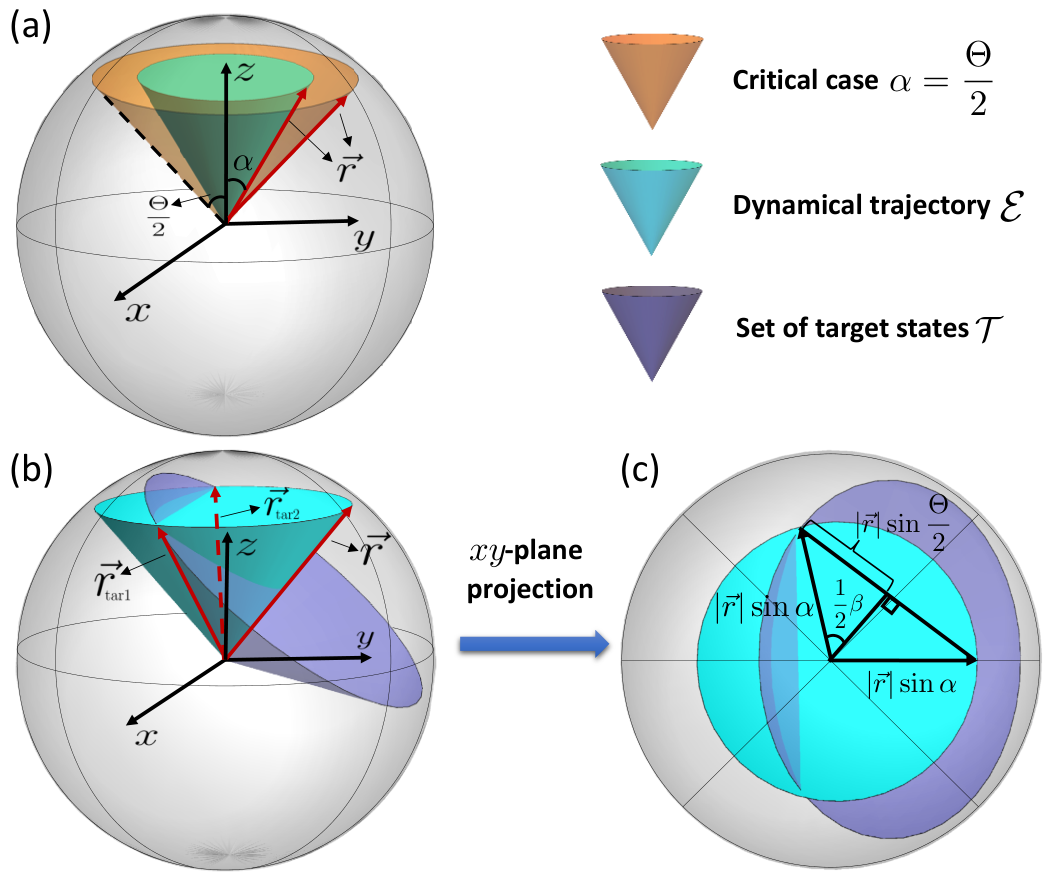
In this appendix we analyze two-level systems. The Hamiltonian of a two-level system in the energy basis is , where , are the energies and , are corresponding eigenstates. Define as , namely, the Pauli matrix in basis . With the Pauli matrix, the Hamiltonian can be rewritten as . The identity matrix commutes with any operator, hence it has nothing to do with the evolution. Then the Hamiltonian can be simplified into . In the Bloch representation, this means the evolution of any state is the rotation of the corresponding Bloch vector about axis. A general vector in the Bloch sphere can be expressed by
| (127) |
where , and . For an initial state , the evolved state is
It can be seen in this equation that the period of the dynamics is
| (128) |
For two-level systems, utilizing Eq. (127), the constrain in given in Proposition 3 reduces to
| (129) |
The states with does not evolve in this case, hence not in the set . For , the condition for to make sure the equation above has solutions for is
| (130) |
which is equivalent to
| (131) |
Furthermore, the minimum time under constrain (129) is reached when is maximum, i.e., , which leads to
| (132) |
Corollary 3 is proved.
To better understand the physics behind the QSL, we analyze the two-level systems from a fully geometric perspective. For any specific initial state , the set of all states on the evolution trajectory (denoted by ) is
| (133) |
One may notice that the set of all target states for a specific initial state (denoted by ) here is a cone with the initial state as the axis and the central angle. For any state , the condition of is that and have intersections.
In the case that , for any specific , as shown in the yellow cone in Fig. 9(a). The coincidence between and means that all the states with in are in the set , i.e., . Furthermore, it is easy to see that for any specific state in this case, only one target state exists, i.e., the symmetrical state with respect to the initial state about -axis. It requires half of the period to rotate the initial state to its symmetrical state, thus, the evolution time in this scenario is
| (134) |
Next, for the case that , all states within (the blue cone in Fig. 9(a)) fail to reach the target since the largest angle between the initial state and the evolved state is , which is smaller than . This means any state satisfying is not in the set .
For the case that , (the blue cone in Fig. 9(b)) for any value of shares two vectors with (the purple cone in Fig. 9(b)), which means any state in this scenario has two target states and on the evolution trajectory. Thus, . Since the rotation is counterclockwise (looking against the axis), the evolution time to is smaller than the one to . To calculate this evolution time, the angle between the projections of and on plane (denoted as ) needs to be known. From Fig. 9(c), it can be found that the length of the projection of is , and the length between these two projections is . Thus, the angle , which indicates that the evolution time is
| (135) |
The minimum value of this evolution time is , which is attained at . Combing the result obtained in the case of , one can finally obtain , and the set . The case with can be analyzed in the same way.
Appendix E The operational definition of the QSL in the Landau-Zener model
The Hamiltonian of Landau-Zener model is
| (136) |
where with the computational basis. and are two time-independent parameters. For the case that , and are the eigenstates of Hamiltonian. The evolution operator for this Hamiltonian can then be calculated as
| (137) |
In the following we will use the traditional notations as the entries of Bloch vector instead of . With above unitary operator, the evolved Bloch vector can be calculated as below
| (138) | |||||
| (139) | |||||
| (140) |
The angle between the initial and evolved states is then of the form
| (141) |
where is the norm of . For the target angle , the evolution time needs to satisfy the equation
| (142) |
In the figure of as a function of , due to the fact that the first extremal value of is 1, which is also the global maximum value, the first crossover point between it and the line is always in the first monotonic increasing regime, in which a smaller value of gives a smaller value of . Therefore, the minimum time satisfying the equation above is attained when is minimum. Due to the fact that , is of the form
| (143) |
which is attained at , i.e., any state in the plane.

The set (in Fig. 5) for all values of in Landau-Zener model is center symmetric about the original point, this is due to the fact the trajectories of two center symmetric states are also center symmetric, as shown in Fig. 10, which means the evolution of the angles between the initial and evolved states are the same for these two states. Therefore they can both reach the target angle simultaneously, which is the reason why is also center symmetric.
Next we calculate the bound Campaioli2018, where
| (144) |
Since , and
| (145) | |||||
Then one can have
| (146) |
In the meantime, , which gives us the final expression of in this case as
| (147) |
When , is a constant, and the equation above reduces to
| (148) |
Appendix F The QSL in open systems
F.1 for the general master equation
For many quantum open systems, the dynamics is governed by the following master equation
| (149) |
where is a -dimensional density matrix, and is th Lindblad operator depicting certain decay mode. Now we calculate the set for this dynamics. Substituting the Bloch representation of into the equation above, one can obtain
| (150) | |||||
Recall that the generators satisfy
| (151) | ||||
| (152) |
where and are some constants. Substituting into both sides of the equation above and taking the trace, one can finally obtain the following equation
| (153) |
which is an affine map with the entries of the coefficients
| (154) | |||||
and
| (155) |
In the case that can be decomposed with the generators, i.e., , the coefficients can be rewritten as
| (156) | |||||
and
| (157) |
For example, the coefficients for reduce to
| (158) | |||||
and .
In the case that and are time-independent, the solution of Eq. (153) is
| (159) |
where satisfies . The inner product between and then reads
| (160) |
Therefore, the general expression of for the above-mentioned master equation is
| (161) |
F.2 Spontaneous emission
Calculation of . Here we show the analysis of the QSL for the dynamics
| (162) | |||||
where and . In the Bloch representation, reads
and . Then the solution is
| (163) |
Rewriting the initial state as
| (164) |
the solutions reduce to
| (165) | |||||
The purity is of the form
| (166) | |||||
In the mean time, the inner product between the initial and evolved states is
| (167) | |||||
Hence, in this case can be expressed by
| (168) |
in which
| (169) |
with and .
Markovian dynamics. Now we consider the case and , which represents the dynamics of the spontaneous emission. In this case, reduces to
| (170) |
Now we assume is very small (in the following we will use instead) and the time to reach the target angle could also be very small. For a very small , approximates to
| (171) |
with which the constrain in Eq. (168) reduces to
| (172) | |||||
Considering the case that , the equation above is equivalent to
| (173) |
which can be rewritten as
| (174) |
For a fixed , the minimum time can be obtained when the left-hand term is maximum. Using the derivative of left-hand term with respect to , one can immediately find out that the maximum value is obtained when , i.e.,
| (175) |
With this optimal initial state, reads
| (176) |
A remarkable fact here is that is propositional to , which means mixed initial states can provide a smaller than pure states.
non-Markovian dynamics. This model (, ) can also reveal the non-Markovian dynamics of damped Jaynes-Cummings models, in which is a time-dependent decay rate. Utilizing an effective Lorentzian spectral density
| (177) |
can be analytically obtained as Deffner2013
| (178) |
where . In this case, the entries of Bloch vector read
where and , are the real and imaginary parts. With these expressions, the norm square of can be calculated as
| (179) |
In the mean time,
which directly gives the set as
| (180) |
where
| (181) |
The numerical calculation suggests that similar to the Markovian dynamics, a lousy purity in this case can also benefit the reduction of . Since is very small here, would also be very small in the case that is not too large. In this case, approximates to , which makes
| (182) |
We also consider the case that , the equation above equals to
| (183) |
which can be rewritten as
| (184) |
For a fixed , the minimum time can be obtained when the left-hand term is maximum, which is the same as the Markovian case, i.e., . With this optimal initial state, we have . Recalling the definition of , one can obtain
| (185) |
which can be further solved as
| (186) |
F.3 Parallel Dephasing
Now we consider the dephasing model, in which the dynamics can be written as
| (187) |
In this case reads
| (188) |
and is a zero vector. Then the dynamics of the Bloch vector reads
| (189) |
Rewriting the initial state as Eq. (164), the solutions reduce to
| (190) |
Since the purity , the inner product between the initial and evolved states is
| (191) |
Hence, is of the form
| (192) |
To provide the regime of in , we need to solve in the constraint condition in Eq. (192). Rewrite it as
| (193) |
where , and . The general solution for the equation above is
To know if the expression of is exactly equivalent to Eq. (192) (since Eq. (193) may bring extra solutions), the sign of
needs to be checked to see if it coincides with . In the case that , is always positive and is only positive when , which means Eq. (192) for is actually equivalent to
| (194) |
Using a similar analysis, one can see that for , Eq. (192) is equivalent to
| (195) |
when and no solution exists for other values of .
Now we discuss the existence of solutions for using Eqs. (194) and (195) instead of Eq. (192). The solutions for exist only when is real and within the regime for some values of . The requirement for real solutions is , which cannot always be satisfied for any value of . When , reduces to , indicating that no state can fulfill the target angle in an extremely small time. Furthermore, when , reduces to . Therefore, the solution of time must be larger than the time () that first let be zero. Around the time , reduces to
| (196) | |||||
For a not very large , always satisfies , which immediately gives , then one can see that
| (197) |
Furthermore, in the same regime that can be satisfied, always holds, which gives
| (198) |
for and for . These two lower bounds can be both lower than 1 for a proper time. Hence, the value of in this regime will continuously reduce to some value smaller than 1 from the time , which means the first cross point between and the regime has to be at 1, which corresponds to the shortest time solution for Eqs. (194) and (195). At this point, the constrain in Eq. (192) reduces to , which immediately gives the QSL as
| (199) |
For example, in the case that , the constrain in Eq. (194) reduces to
| (200) |
For a not very large , the smallest value of the right-hand side expression is , which can be reached at . And it is obvious that its value can larger than 1; therefore, the regime of in which the above equation has solutions for is , which directly leads to the regime of in as
and the QSL is .
References
- (1) E. Chitambar and G. Gour, Quantum resource theories, Rev. Mod. Phys. 91, 025001 (2019).
- (2) V. Giovannetti, S. Lloyd and L. Maccone, Advances in quantum metrology, Nat. Photon. 5 222–9 (2011).
- (3) G. Tóth and I. Apellaniz, Quantum metrology from a quantum information science perspective, J. Phys. A: Math. Theor. 47, 424006 (2014).
- (4) L. Mandelstam and I. Tamm, The uncertainty relation between energy and time in nonrelativistic quantum mechanics, J. Phys. 9, 249 (1945).
- (5) N. Margolus and L. B. Levitin, The maximum speed of dynamical evolution, Physica D 120, 188 (1998).
- (6) V. Giovannetti, S. Lloyd and L. Maccone, The speed limit of quantum unitary evolution, J. Opt. B 6, 807 (2004).
- (7) L. B. Levitin and T. Toffoli, Fundamental Limit on the Rate of Quantum Dynamics: The Unified Bound Is Tight, Phys. Rev. Lett. 103, 160502 (2009).
- (8) Y.-J. Zhang, W. Han, Y.-J. Xia, J.-P. Cao and H. Fan, Quantum speed limit for arbitrary initial states, Sci. Rep. 4, 4890 (2014).
- (9) D. Mondal, C. Datta, S. Sazim, Quantum coherence sets the quantum speed limit for mixed states, Phys. Lett. A 380, 689-695 (2016).
- (10) D. P. Pires, M. Cianciaruso, L. C. Céleri, G. Adesso and D. O. Soares-Pinto, Generalized Geometric Quantum Speed Limits, Phys. Rev. X 6, 021031 (2016).
- (11) I. Marvian, R. W. Spekkens and P. Zanardi, Quantum speed limits, coherence, and asymmetry Phys. Rev. A 93, 052331 (2016).
- (12) S. Deffner and S. Campbell, Quantum speed limits: from Heisenberg’s uncertainty principle to optimal quantum control, J. Phys. A: Math. Theor. 50, 453001 (2017).
- (13) J. M. Epstein and K. B. Whaley, Quantum speed limits for quantum-information-processing tasks, Phys. Rev. A 95, 042314 (2017).
- (14) F. Campaioli, F. A. Pollock, F. C. Binder and K. Modi, Tightening Quantum Speed Limits for Almost All States, Phys. Rev. Lett. 120, 060409 (2018).
- (15) M. Bukov, D. Sels, and A. Polkovnikov, Geometric Speed Limit of Accessible Many-Body State Preparation, Phys. Rev. X 9, 011034 (2019).
- (16) S.-x. Wu and C.-s. Yu, Quantum speed limit for a mixed initial state, Phys. Rev. A 98, 042132 (2018).
- (17) C. Liu, Z.-Y. Xu and S. Zhu, Quantum-speed-limit time for multiqubit open systems, Phys. Rev. A 91, 022102 (2015).
- (18) S. Ashhab, P. C. de Groot and F. Nori, Speed limits for quantum gates in multiqubit systems, Phys. Rev. A 85, 052327 (2012).
- (19) Y.-J. Zhang, W. Han, Y.-J. Xia, J.-P. Cao and H. Fan, Classical-driving-assisted quantum speed-up, Phys. Rev. A 91, 032112 (2015).
- (20) M. M. Taddei, B. M. Escher, L. Davidovich and R. L. de Matos Filho, Quantum Speed Limit for Physical Processes, Phys. Rev. Lett. 110 050402 (2013).
- (21) A. del Campo, I. L. Egusquiza, M. B. Plenio and S. F. Huelga, Quantum Speed Limits in Open System Dynamics, Phys. Rev. Lett. 110 050403 (2013).
- (22) S. Deffner, E. Lutz, Quantum Speed Limit for Non-Markovian Dynamics, Phys. Rev. Lett. 111 010402 (2013).
- (23) Z. Sun, J. Liu, J. Ma and X. Wang, Quantum speed limit for Non-Markovian dynamics without rotating-wave approximation, Sci. Rep. 5, 8444 (2015).
- (24) I. Marvian and D. A. Lidar, Quantum Speed Limits for Leakage and Decoherence, Phys. Rev. Lett. 115, 210402 (2015).
- (25) N. Mirkin, F. Toscano and D. A. Wisniacki, Quantum-speed-limit bounds in an open quantum evolution, Phys. Rev. A 94, 052125 (2016).
- (26) L. P. García-Pintos and A. del Campo, Quantum speed limits under continuous quantum measurements, New J. Phys. 21, 033012 (2019).
- (27) F. Campaioli, F. A. Pollock and K. Modi, Tight, robust, and feasible quantum speed limits for open dynamics, Quantum 3, 168 (2019).
- (28) A. Chenu, M. Beau, J. Cao, A. del Campo, Quantum Simulation of Generic Many-Body Open System Dynamics Using Classical Noise, Phys. Rev. Lett. 118, 140403 (2017).
- (29) M. Beau, J. Kiukas, I. L. Egusquiza, A. del Campo, Nonexponential quantum decay under environmental decoherence, Phys. Rev. Lett. 119, 130401 (2017).
- (30) V. Giovannetti, S. Lloyd and L. Maccone, Quantum limits to dynamical evolution, Phys. Rev. A 67, 052109 (2003)
- (31) V. Giovannetti, S. Lloyd and L. Maccone, Quantum Metrology, Phys. Rev. Lett. 96, 010401 (2006).
- (32) M. Beau and A. del Campo, Nonlinear quantum metrology of many-body open systems, Phys. Rev. Lett. 119, 010403 (2017).
- (33) T. Caneva, M. Murphy, T. Calarco, R. Fazio, S. Montangero, V. Giovannetti and G. E. Santoro, Optimal Control at the Quantum Speed Limit, Phys. Rev. Lett. 103, 240501 (2009).
- (34) G. C. Hegerfeldt, Driving at the Quantum Speed Limit: Optimal Control of a Two-Level System, Phys. Rev. Lett. 111, 260501 (2013).
- (35) K. Funo, J.-N. Zhang, C. Chatou, K. Kim, M. Ueda, A. del Campo, Universal Work Fluctuations During Shortcuts to Adiabaticity by Counterdiabatic Driving, Phys. Rev. Lett. 118, 100602 (2017).
- (36) S. Campbell and S. Deffner, Trade-Off Between Speed and Cost in Shortcuts to Adiabaticity Phys. Rev. Lett. 118, 100601 (2017).
- (37) P. M. Poggi, Geometric quantum speed limits and short-time accessibility to unitary operations, Phys. Rev. A 99, 042116 (2019).
- (38) D. Girolami, How Difficult is it to Prepare a Quantum State? Phys. Rev. Lett. 122, 010505 (2019).
- (39) X. Cai and Y. Zheng, Quantum dynamical speedup in a nonequilibrium environment, Phys. Rev. A 95, 052104 (2017).
- (40) D. V. Villamizar and E. I. Duzzioni, Quantum speed limit for a relativistic electron in a uniform magnetic field, Phys. Rev. A 92, 042106 (2015).
- (41) S. Sun and Y. Zheng, Distinct Bound of the Quantum Speed Limit via the Gauge Invariant Distance, Phys. Rev. Lett. 123, 180403 (2019).
- (42) N. Margolus, The finite-state character of physical dynamics, arXiv:1109.4994 (2011).
- (43) B. Shanahan, A. Chenu, N. Margolus and A. del Campo, Quantum Speed Limits across the Quantum-to-Classical Transition, Phys. Rev. Lett. 120, 070401 (2018).
- (44) M. Okuyama and M. Ohzeki, Quantum Speed Limit is Not Quantum, Phys. Rev. Lett. 120, 070402 (2018).
- (45) S. Amari, Information Geometry and Its Applications, Applied Mathematical Sciences 194, (Springer Japan, 2016).
- (46) X.-M. Zhang, Z.-W. Cui, X. Wang and M.-H. Yung, Automatic spin-chain learning to explore the quantum speed limit, Phys. Rev. A 97, 052333 (2018).
- (47) J. Liu, H. Yuan, X.-M. Lu and X. Wang, Quantum Fisher information matrix and multiparameter estimation, J. Phys. A: Math. Theor. 53, 023001 (2020).
- (48) D. Petz, Monotone metrics on matrix spaces, Linear Algebr. Appl. 244, 81 (1996).
- (49) L. Zhang, Y. Sun and S. Luo, Quantum speed limit for qubit systems: Exact results Phys. Lett. A 382, 2599-2604 (2018).
- (50) M. A. Nielsen and I. L. Chuang, Quantum Computation and Quantum Information (Cambridge University Press, Cambridge, 2000).
- (51) M. Heyl, Quenching a quantum critical state by the order parameter: Dynamical quantum phase transitions and quantum speed limits, Phys. Rev. B 95, 060504(R) (2017).
- (52) X. Meng, C. Wu and H. Guo, Minimal evolution time and quantum speed limit of non-Markovian open systems, Sci. Rep. 5, 16357 (2015).
- (53) N. Mirkin, M. Larocca and D. Wisniacki, Quantum metrology in a non-Markovian quantum evolution, arXiv:1912.04675 (2019).
- (54) Q. Bin, X.-Y. Lü, F. P. Laussy, F. Nori and Y. Wu, N-Phonon Bundle Emission via the Stokes Process, Phys. Rev. Lett. 124, 053601 (2020).