oddsidemargin has been altered.
textheight has been altered.
marginparsep has been altered.
textwidth has been altered.
marginparwidth has been altered.
marginparpush has been altered.
The page layout violates the UAI style.
Please do not change the page layout, or include packages like geometry, savetrees, or fullpage, which change it for you.
We’re not able to reliably undo arbitrary changes to the style. Please remove the offending package(s), or layout-changing commands and try again.
Efficient Rollout Strategies for Bayesian Optimization
Abstract
Bayesian optimization (BO) is a class of sample-efficient global optimization methods, where a probabilistic model conditioned on previous observations is used to determine future evaluations via the optimization of an acquisition function. Most acquisition functions are myopic, meaning that they only consider the impact of the next function evaluation. Non-myopic acquisition functions consider the impact of the next function evaluations and are typically computed through rollout, in which steps of BO are simulated. These rollout acquisition functions are defined as -dimensional integrals, and are expensive to compute and optimize. We show that a combination of quasi-Monte Carlo, common random numbers, and control variates significantly reduce the computational burden of rollout. We then formulate a policy-search based approach that removes the need to optimize the rollout acquisition function. Finally, we discuss the qualitative behavior of rollout policies in the setting of multi-modal objectives and model error.
1 INTRODUCTION
Bayesian optimization (BO) is a class of methods for global optimization used to minimize expensive black-box functions. BO builds a probabilistic surrogate model of the objective and then determines future evaluations via an acquisition function. Applications of BO include robotic gait control, sensor set selection, and neural network hyperparameter tuning [21, 22, 3]. BO is favored in these tasks because of its sample-efficient nature. Achieving this sample-efficiency demands that BO balance exploration and exploitation. However, standard acquisition functions such as expected improvement (EI) are too greedy and perform little exploration. As a result, they perform poorly on multimodal problems [7] and have provably sub-optimal performance in certain settings, e.g., bandit problems [23]. A key research goal in BO is developing less greedy acquisition functions [21]. Examples include predictive entropy search (PES) [7] or knowledge gradient (KG) [4]. Lam et al. 2016 frame the exploration-exploitation trade-off as a balance between immediate and future rewards in a continuous state and action space Markov decision process (MDP). In this framework, non-myopic acquisition functions are optimal MDP policies, and promise better performance by considering the impact of future evaluations up to a given BO budget (also referred to as the horizon).

Unfortunately, maximizing the MDP reward is an intractable problem as it involves solving an infinite-dimensional dynamic program [18]. Rollout is a popular class of approximate solutions in which future BO realizations and their corresponding values are simulated using the surrogate and then averaged. This average defines a rollout acquisition function, which is considered the state-of-the-art in non-myopic BO. While more practical than the original MDP problem, rollout acquisition functions are still computationally expensive to the extent that suggesting the next evaluation can take several hours [24]. This paper aims to make non-myopic BO more practical by reducing the time to suggest the next point from hours to seconds. In particular, our main contributions are:
- •
We compute rollout acquisition functions via Monte Carlo integration, and use variance reduction techniques —quasi-Monte Carlo, common random numbers, and control variates— to decrease the estimation error by several orders of magnitude.
- •
We introduce a coarser approximation to rollout acquisition functions through policy search. In this setting, we use rollout to select the best acquisition function from a given set at each BO iteration. This removes the need to optimize the rollout acquisition function, and makes rollout much more practical.
- •
We provide experimental results for both rollout acquisitions and policy search. The former suggests that rollout acquisition functions perform better on multimodal problems. The latter shows that policy search performs as well as, if not better than, the best-performing one-step acquisition function.
- •
We examine the impact of model mis-specification on performance and show that increasing the rollout horizon also increases sensitivity to model error.
2 BACKGROUND
Many papers have been published in the sub-field of non-myopic BO over the last few years [5, 6, 14, 15, 16, 24, 25]. Most of this recent research concerns rollout, in which future realizations of BO are simulated over horizon using the surrogate and averaged to determine the acquisition function. Rollout acquisition functions represent the state-of-the-art in BO and are integrals over dimensions, where the integrand itself is evaluated through inner optimizations, resulting in an expensive integral. The rollout acquisition function is then maximized to determine the next BO evaluation, further increasing the cost. This large computational overhead is evidenced by Osborne et al. 2009, who are only able to compute the rollout acquisition for horizon 2, dimension 1; and later by Lam et al. 2016, who use Gauss-Hermite quadrature in horizons up to five and see runtimes on the order of hours for small, synthetic functions [24].
Recent work focuses on making rollout more practical. Wu and Frazier 2019 consider horizon two and use a combination of Gauss-Hermite quadrature and Monte Carlo (MC) integration to quickly calculate the acquisition function and its gradient. Non-myopic active learning also uses rollout and recent work develops a fast implementation by truncating the horizon and selecting a batch of points to collect future rewards [10, 11].

Gaussian process regression and BO: Suppose we seek a global minimum of a continuous objective over a compact set . If is expensive to evaluate, finding a minimum should ideally be sample-efficient. BO often uses a Gaussian process (GP) to model from the data . The next evaluation location is determined by maximizing an acquisition function : .
We place a GP prior on , denoted by , where and are the mean function and covariance kernel, respectively (see the supplement for examples). The kernel correlates neighboring points, and may contain hyperparameters, such as lengthscales that are learned to improve the quality of approximation [20]. For a given , we define:
We assume is observed with Gaussian white noise: , where . Given a GP prior and data , the resulting posterior distribution for function values at a location is the Normal distribution :
where .
Non-myopic Bayesian optimization: Non-myopic BO frames the exploration-exploitation trade-off as a balance of immediate and future rewards. The strength of this approach is demonstrated in Figure 1, in which we compare EI and KG to a non-myopic acquisition function on a carefully chosen objective. Its GP has a region of uncertainty on the left containing the global minimum and a local minimum at the origin. We run two steps of BO, updating the posterior each step. EI and KG behave greedily by sampling twice near the origin, while the non-myopic approach uses one evaluation to explore the uncertain region, subsequently identifying the global minimum and converging faster than either EI or KG.
Lam et al. 2016 formulate non-myopic BO as a finite horizon dynamic program. We present the equivalent Markov decision process (MDP) formulation. We use standard notation from Puterman [19]: an MDP is the collection . , is the set of decision epochs, assumed finite for our problem. The state space, , encapsulates all the information needed to model the system from time . is the action space. Given a state and an action , is the transition probability of the next state being . is the reward received for choosing action from state , and ending in state .
A decision rule, , maps states to actions at time . A policy is a series of decision rules , one at each decision epoch. Given a policy , a starting state , and horizon , we can define the expected total reward as:
In phrasing a sequence of decisions as an MDP, our goal is to find the optimal policy that maximizes the expected total reward, i.e., , where is the space of all admissible policies.
If we can sample from the transition probability , we can estimate the expected total reward of any base policy with MC integration:
Given a GP prior over data with mean and kernel , we model steps of BO as an MDP. This MDP’s state space is all possible data sets reachable from starting state with steps of BO. Its action space is ; actions correspond to sampling a point in . Its transition probability and reward function are defined as follows. Given an action , the transition probability from to , where is:
In other words, the transition probability from to is the probability of sampling from the posterior at . We define a reward according to EI [12]. Let be the minimum observed value in the observed set , i.e., . Then our reward is expressed as:
EI can be defined as the optimal policy for horizon one, obtained by maximizing the immediate reward:
where the starting state is . In contrast, we define the non-myopic policy as the optimal solution to an -horizon MDP. The expected total reward of this MDP can be expressed as:
For , the optimal policy is difficult to compute.
Rollout acquisition functions: In the context of BO, rollout policies [1], which are sub-optimal but yield promising results, are a tractable alternative to optimal policies [24]. For a given current state , we denote our base policy . We introduce the notation to define the initial state of our MDP and for to denote the random variable that is the state at each decision epoch. Each individual decision rule consists of maximizing the base acquisition function given the current state ,
Using this policy, we define the non-myopic acquisition function as the rollout of to horizon i.e., the expected reward of starting with the action :
where is the noisy observed value of at . is better than in expectation for a correctly specified GP prior and for any acquisition function. This follows from standard results in the MDP literature:
Definition 2.1
Bertsekas 2017: A policy is sequentially consistent if, for every trajectory generated from any :
generates the following trajectory starting at :
Sequential consistency requires the trajectory generated from applying at for horizon to be a sub-trajectory of the trajectory generated from applying at for horizon . Acquisition functions are sequentially consistent so long as we consistently break ties if they have multiple maxima —though this will not occur generically. Sequential consistency guarantees that rollout does at least as well as its base policy in expectation:
Theorem 2.1
Bertsekas 2017: A rollout policy does as least as well as its base policy in expectation if is sequentially consistent i.e.,
Thus, rolling out any acquisition function will do at least as well in expectation as the acquisition function itself.
Unfortunately, while rollout is tractable and conceptually straightforward, it is computationally demanding. To rollout once, we must run steps of BO with . Many such rollouts must then be averaged to reasonably estimate , which is an -dimensional integral. Estimation can be done either through explicit quadrature or MC integration, and is the primary computational bottleneck of rollout. Our paper significantly lowers the computational burden of rollout through MC variance reduction and a fast policy search method that avoids optimizing . We detail these methods in the next section.
3 METHODS
In the context of rollout, MC estimates the expected reduction over steps of BO using base policy :
The distribution for is a normal distribution whose mean and variance are determined by rolling out to horizon and examining the posterior GP:
| (1) | ||||
A sample path in this context may be represented as the sequence produced by Equation 1. We parameterize the vector of values, , with an -dimensional vector drawn from . is distributed according to , so we map to by a simple scale-and-shift. This map is done sequentially from time step one to time step . MC integration thus involves sampling times from , mapping each of the samples, and averaging. The mapping step is equivalent to applying our rollout policy , and is the dominant cost of integration.
Compared to other quadrature schemes, MC is well-suited to high-dimensional integration. MC converges at a rate of , the standard deviation of the MC estimator, where is the sample variance and is the total number of samples. MC’s primary drawback is slow convergence. Increasing precision by an order of magnitude requires two orders of magnitude more samples. If is high, many samples may be required to converge. In this section, we focus on two strategies that significantly decrease the overhead of rollout: variance reduction and policy search.
3.1 Variance reduction

Variance reduction is a class of methods that improve convergence by decreasing the variance of the estimator. Effective variance reduction methods can reduce by orders of magnitude. We use a combination of quasi-Monte Carlo, common random numbers, and control variates, which significantly reduces the number of MC samples needed, as evidenced by Figure 2.
Quasi-Monte Carlo (QMC): Instead of sampling directly from the probability distribution, QMC instead uses a low-discrepancy sequence as its sample set.
Theorem 3.1
Caflisch 1998: QMC converges at a rate bounded above by , where is the number of samples and is the integral’s dimension.
This bound stems from the well-known Koksma-Hlawka inequality [2], and is roughly linear for large . In practice, this bound is often loose and convergence proceeds faster [17]. QMC is inapplicable if a low-discrepancy sequence does not exist for the target distribution.
In our case, the distributions we integrate over are Normal, for which low-discrepancy sequences do exist. We generate low-discrepancy Sobol sequences in the -dimensional uniform distribution and map them to the unit multivariate Gaussian via the Box-Muller transform. This yields a low-discrepancy sequence for . Recall the parameterization of samples from to sample rollout trajectories in Equation 1. We apply QMC by replacing the unit multivariate Gaussian samples with our low-discrepancy sequence.

Common random numbers (CRN): CRN is used when estimating a quantity to be optimized over parameter , and is implemented by using the same random number stream for all values of . CRN does not decrease the point-wise variance of an estimate, but rather decreases the covariance between two neighboring estimates, which smooths out the function. Consider estimating and for two points and using samples, with variances and respectively. We define the differences and as:
uses the same number stream for and . If and are close and is continuous in , , implying . This increased consistency between neighboring points improves optimization accuracy, as seen in Figure 3.
Control variates: The general idea behind control variates is to find a covariate with the same distribution as and a known mean. The quantity , known as a regression control variate (RCV), is estimated, and then de-biased afterwards.
Theorem 3.2
Consider the estimator . Let . is sufficiently correlated with if:
If is sufficiently correlated with , then the estimator is strictly more accurate than i.e., .
The optimal value that minimizes the variance of is . In practice, both and must be estimated. This formula generalizes to multiple control variates (included in the supplementary). We note that variates whose derivatives are also correlated with the derivatives of yield superior performance, especially when using QMC [8].
In the context of BO, we opt to use covariates derived from existing acquisition functions with known means. EI and PI are straightforward options. We expect their value to be at least somewhat correlated with the value of the rollout acquisition function; a promising candidate point should ideally score highly among all acquisition functions, and vice-versa. We will demonstrate the effectiveness of these variates in Section 4. EI and PI are defined as the expectation of a random variable of the form :
- •
Probability of improvement (PI)
- •
Expected improvement (EI)
3.2 Policy search
While we have dramatically lowered the cost of evaluating the rollout acquisition function, there still remains the problem of its optimization. Wu and Frazier 2019 use the reparameterization trick to estimate the gradient of EI for horizon two and use stochastic gradient descent to maximize it. However, their method does not immediately extend to horizons larger than two.
Policy search is an alternative method for approximately solving MDPs, in which a best performing policy is chosen out of a (possibly infinite) set of policies [1]. It is performed either by computing the expected reward for each policy in the set, or using a gradient-based method to maximize the expected reward given a parameterization of the policy set. In this paper, we use a finite policy set:
where is any arbitrary set of acquisition functions. We then select the best-performing policy:
A less formal explanation follows: at every step of BO, we roll out each acquisition function in on its argmax, and use the one with the highest -step reward. A related approach by Hoffman et al. 2011 employs a bandit strategy to switch between different acquisition functions. Our policy search method does not maximize the rollout acquisition function, and is thus significantly faster, though it likely reduces performance. Experiments in Section 4 suggest that our policy search method performs at least as well as the best-performing acquisition in .
4 EXPERIMENTS AND DISCUSSION

Unless otherwise stated, we use a GP with the Matérn ARD kernel [22] and learn its hyperparameters via maximum likelihood estimation [20]. When rolling out acquisition functions, we maximize them with L-BFGS-B using five restarts, selected by evaluating the acquisition on a Latin hypercube of points and picking the five best. EI is used as the base rollout policy except for in the policy search experiments. All synthetic functions are found in the supplementary. Code to reproduce our experiments is found at https://github.com/ericlee0803/lookahead_release.
Variance reduction experiments: We compare the estimation error and convergence rate between the standard MC estimator and our estimator. We take random points in the domain and evaluate the Ackley and Rastrigin functions in D and D, respectively. We roll out EI for horizons , , , and , and calculate the variance of both estimators for MC sample sizes in , using trials each. We take the ground truth to be estimation with samples. The mean error of the standard MC estimator (red) and our reduced-variance estimator (blue) are plotted with dotted lines in Figure 4, with standard error shaded above and below. We also compute a best-fit line to each mean error, which is plotted with a solid line.
| Objective | Horizon | MC Rate | Our Rate | |
|---|---|---|---|---|
| Ackley | ||||
| Ackley | ||||
| Ackley | ||||
| Ackley | ||||
| Rastrigin | ||||
| Rastrigin | ||||
| Rastrigin | ||||
| Rastrigin |
Table 1 summarizes our experimental results, and includes our estimates for the convergence rate of both estimators and the relative reduction in estimation error . Our estimator has significantly lower estimation error —the maximum reduction in estimation error we achieve is a factor of . Standard MC clearly converges at a rate. Our estimator converges like for smaller horizons, but its convergence rate drops as increases. This is due to QMC’s convergence. is not large enough for longer horizons to exhibit convergence; increasing it past should yield convergence.
Another trend is the increase in estimation error as the horizon increases, which is expected given that the dimensionality of the underlying integral increases. Fortunately, the error seems to increase only linearly —and by a small constant— rather than exponentially, suggesting that MC samples proportional to is sufficient to achieve a high quality of approximation. Finally, the reduction in estimation error levels off to around a factor of , suggesting that the correlation between the rollout acquisition function and our control variates decreases when increases. We include an ablation study in the supplement to quantify the individual contributions of QMC and control variates.
A factor of 25 error reduction is still significant; the standard MC estimator would need times more samples to achieve comparable accuracy.


Full rollout on synthetic functions: We roll out EI for , and on the Branin, weighted-two-norm (D), Ackley (D), and Rastrigin (D) functions in Figure 5 using MC samples, and compare to both standard EI and random search. To optimize the acquisition functions quickly, we employ the following strategy: we evaluate the acquisition function on a Sobel sequence of size , as well as an additional point which is the argmax of EI. We then use this as an initial design and run BO for more iterations. We run iterations for each horizon and provide random search as a baseline. The mean results and the standard error are plotted in Figure 5.
On the Branin function, all horizons performed comparably and converge in iterations. Rollout performed best on the Ackley and Rastrigin functions, which are multimodal. On the weighted norm function, which is strongly convex, EI converges within iterations, and looking ahead further yielded poorer results. These results suggest that more exploratory acquisitions are needed for a multimodal objective, whereas more exploitative acquisitions suffice for reasonably simple objective functions.
Policy search: We consider policy search (PS) with an acquisition set of EI, KG, and Upper Confidence Bound (UCB–) for [22], which contains acquisitions that tend towards both exploitation and exploration. We run policy search for horizons and on the Branin, Sixhump, Ackley, and Rastrigin synthetic functions, all in D, using MC samples.
All acquisition functions are maximized via L-BFGS-B with five random restarts, except for KG, which uses grid search of size . The mean results and standard error over trials are plotted in Figure 6, in which policy search for horizons and , labeled PS and PS respectively, do better or on par with the best-performing acquisition function. This robustness is a key strength of policy search, as the performance of each acquisition function is often problem-dependent.

We also examine the choice of acquisition function as a function of iteration. The percentage of use of each acquisition function is shown for its corresponding objective, and for plotting purposes we smooth the percentage with a box filter of size five. EI and KG are chosen more often than the other acquisition functions. UCB-, the worst performing method representing a pure exploitation policy, is chosen significantly less than others, while UCB- was chosen the most often out of the UCB family. Of particular interest is the Ackley function (third column, Figure 6): when UCB- starts to outperform the other acquisitions functions, a clear spike in its percentage of use is seen in the corresponding histogram.
Neural architecture search (NAS) benchmark: We run policy search on the NAS tabular benchmarks in [13], which are an exhaustive set of evaluated configurations for multi-layer perceptrons trained on different datasets. We optimizer the perceptrons’ layer sizes, batch size, and training epochs with 60 iterations of BO for each dataset and plot average regret in Figure 8. For space’s sake, we describe the search space and the regret metric in the supplement. Policy search for and performs better than EI, UCB0, UCB2, and KG.

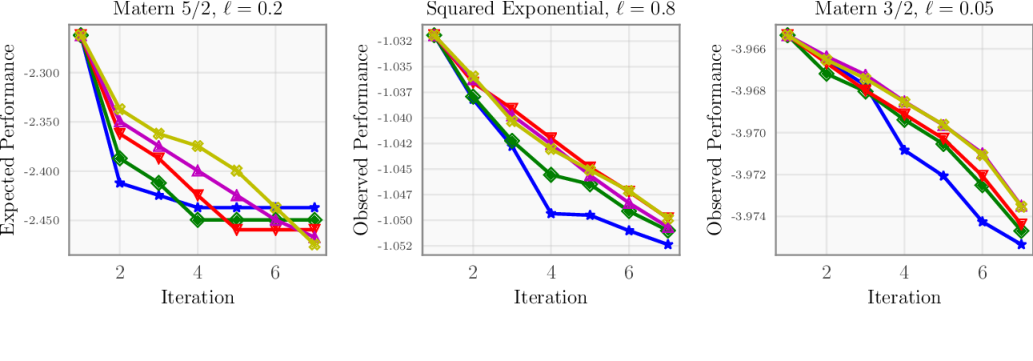
The impact of model mis-specification: We believe that any probabilistic model only supports a limited horizon due to the effects of model error. Errors in the GP model result in errors to the MDP transition probabilities, which grow as they are propagated through time. This likely renders long-horizon rollout ineffectual. We support this hypothesis by comparing the performance of policies in the MDP setting they were designed in with their observed performance on objectives drawn from a different MDP.
We do this by drawing objective functions from a GP with fixed kernel every step of BO. More concretely, evaluating the objective function at any point is performed by sampling from the GP posterior distribution at . Because policies are designed to maximize this MDP’s reward for a fixed horizon and because the objective is drawn from the MDP itself, policies looking further ahead perform better by definition. We then draw objectives from a GP using a different kernel with a different lengthscale, and check if policies looking further ahead still perform better.
We rollout EI in D with a budget of seven and we model our objective with a GP using the Matérn kernel with . In Figure 7, the left panel depicts expected performance of rollout for = , , , , and . The middle and right panels depict observed performance of rollout when the we sample objectives from a GP that has a far smoother kernel (Square Exponential with ) and far less smooth kernel (Matérn with ), respectively. All plots use replications to achieve high accuracy.
The result is perhaps unsurprising; the ranking of the observed performance of policies is reversed with that of the expected performance. Myopic BO performed the best; more generally, policies with shorter horizons outperformed those with longer horizons. This demonstrated sensitivity to model error suggests non-myopic BO must carefully strike a balance between model accuracy and horizon, and justifies use of modest horizons over the full BO budget. This confirms experimental results by Yue and Kontar 2020, who suggest looking ahead to short horizons is preferable to long horizons in practice.
5 CONCLUSION
We have shown that a combination of quasi-Monte Carlo, control variates, and common random numbers significantly lowers the overhead of rollout in BO. We have introduced a policy search which further decreases computational cost by removing the need to maximize the rollout acquisition function. Finally, we have illustrated the penalties incurred by using inaccurate GP models in the non-myopic setting.
This work raises several interesting research directions. Decreasing the variance of our estimator may be possible with additional variance reduction methods such as stratified or antithetic sampling. Developing a more comprehensive policy search space, such as a parameterized set of all convex combinations of acquisition functions, may further strengthen the policy search performance.
References
- Bertsekas [2017] D. P. Bertsekas. Dynamic Programming and Optimal Control, volume I. Athena scientific Belmont, MA, 4th edition, 2017.
- Caflisch [1998] R. E. Caflisch. Monte Carlo and quasi-Monte Carlo methods. Acta numerica, 7:1–49, 1998.
- Frazier [2018] P. I. Frazier. Bayesian optimization. In E. Gel and L. Ntaimo, editors, Recent Advances in Optimization and Modeling of Contemporary Problems, pages 255–278. INFORMS, 2018. doi: 10.1287/educ.2018.0188.
- Frazier et al. [2008] P. I. Frazier, W. B. Powell, and S. Dayanik. A knowledge-gradient policy for sequential information collection. SIAM Journal on Control and Optimization, 47(5):2410–2439, 2008.
- Ginsbourger and Le Riche [2010] D. Ginsbourger and R. Le Riche. Towards Gaussian process-based optimization with finite time horizon. In Proceedings of the 9th International Workshop in Advances in Model-Oriented Design and Analysis, pages 89–96. Springer, 2010.
- González et al. [2016] J. González, M. A. Osborne, and N. Lawrence. GLASSES: Relieving the myopia of Bayesian optimisation. In Artificial Intelligence and Statistics, pages 790–799, 2016.
- Hernández-Lobato et al. [2014] J. M. Hernández-Lobato, M. W. Hoffman, and Z. Ghahramani. Predictive entropy search for efficient global optimization of black-box functions. In Proceedings of the 28th Conference on Neural Information Processing Systems, pages 918–926, 2014.
- Hickernell et al. [2005] F. J. Hickernell, C. Lemieux, A. B. Owen, et al. Control variates for quasi-monte carlo. Statistical Science, 20(1):1–31, 2005.
- Hoffman et al. [2011] M. D. Hoffman, E. Brochu, and N. de Freitas. Portfolio allocation for Bayesian optimization. In UAI, pages 327–336. Citeseer, 2011.
- Jiang et al. [2017] S. Jiang, G. Malkomes, G. Converse, A. Shofner, B. Moseley, and R. Garnett. Efficient nonmyopic active search. In Proceedings of the 34th International Conference on Machine Learning, pages 1714–1723, 2017.
- Jiang et al. [2018] S. Jiang, G. Malkomes, M. Abbott, B. Moseley, and R. Garnett. Efficient nonmyopic batch active search. In Proceedings of the 32nd Conference on Neural Information Processing Systems, pages 1107–1117, 2018.
- Jones et al. [1998] D. R. Jones, M. Schonlau, and W. J. Welch. Efficient global optimization of expensive black-box functions. Journal of Global Optimization, 13(4):455–492, 1998. ISSN 1573-2916.
- Klein and Hutter [2019] A. Klein and F. Hutter. Tabular benchmarks for joint architecture and hyperparameter optimization. arXiv preprint arXiv:1905.04970, 2019.
- Lam and Willcox [2017] R. Lam and K. Willcox. Lookahead Bayesian optimization with inequality constraints. In Proceedings of the 31st Conference on Neural Information Processing Systems, pages 1890–1900, 2017.
- Lam et al. [2016] R. Lam, K. Willcox, and D. H. Wolpert. Bayesian optimization with a finite budget: An approximate dynamic programming approach. In Proceedings of the 30th Conference on Neural Information Processing Systems, pages 883–891, 2016.
- Osborne et al. [2009] M. A. Osborne, R. Garnett, and S. J. Roberts. Gaussian processes for global optimization. In Proceedings of the 3rd International Conference on Learning and Intelligent Optimization (LION3), pages 1–15, 2009.
- Papageorgiou [2003] A. Papageorgiou. Sufficient conditions for fast quasi-Monte Carlo convergence. Journal of Complexity, 19(3):332–351, 2003.
- Powell [2007] W. B. Powell. Approximate Dynamic Programming: Solving the Curses of Dimensionality. Wiley, 2nd edition, 2007.
- Puterman [2014] M. L. Puterman. Markov Decision Processes: Discrete Stochastic Dynamic Programming. John Wiley & Sons, Inc., 2014.
- Rasmussen and Williams [2006] C. E. Rasmussen and C. K. Williams. Gaussian Processes for Machine Learning. MIT Press, 2006.
- Shahriari et al. [2016] B. Shahriari, K. Swersky, Z. Wang, R. P. Adams, and N. de Freitas. Taking the human out of the loop: A review of Bayesian optimization. Proceedings of the IEEE, 104(1):148–175, Jan 2016.
- Snoek et al. [2012] J. Snoek, H. Larochelle, and R. P. Adams. Practical Bayesian optimization of machine learning algorithms. In Proceedings of the 26th Conference on Neural Information and Processing Systems, pages 2951–2959, 2012.
- Srinivas et al. [2010] N. Srinivas, A. Krause, S. Kakade, and M. Seeger. Gaussian process optimization in the bandit setting: No regret and experimental design. Proceedings of the 27th International Conference on Machine Learning, pages 1015–1022, 2010.
- Wu and Frazier [2019] J. Wu and P. Frazier. Practical two-step lookahead Bayesian optimization. In Advances in Neural Information Processing Systems, pages 9810–9820, 2019.
- Yue and Kontar [2020] X. Yue and R. A. Kontar. Why non-myopic Bayesian optimization is promising and how far should we look-ahead? A study via rollout. Artificial Intelligence and Statistics, 2020.
Appendix
Appendix A KERNELS
The kernel functions we use in this paper are the squared exponential (SE) kernel, Matérn 5/2 kernel, and Matérn 3/2 kernel, respectively:
where .
Appendix B ACQUISITION FUNCTIONS
PI, EI, and UCB- have the closed forms:
KG does not have a closed form. It is defined as the expected value of the posterior minimum:
Where is the value of the the posterior mean having sampled at . The distribution of is the posterior distribution of the GP.
Appendix C CONTROL VARIATES
The general idea behind control variates is to find a covariate with known mean and negative correlation with . The quantity , known as a regression control variate (RCV), is estimated, and then de-biased afterwards. If and , then:
The optimal value minimizing the variance of is thus:
In practice, both and must be either estimated from samples of and or computed a-priori.
In the case of control variates, we consider a vector of control variates . Our estimator will have the form , where is an length vector of constants. The optimal minimizing the variance of is:
where is the covariance matrix of and is the vector of covariances between each variate and .


Appendix D NAS BENCHMARK
The NAS benchmark is a tabular benchmark containing all possible hyperparameter configurations evaluated for a two-layer multi-layer perceptron on different datasets. The search space we consider is:
- •
Batch size in .
- •
Epochs in .
- •
Layer 1 width in .
- •
Layer 2 width in .
The resulting search space is four-dimensional. We optimize over the unit hypercube and scale and round evaluation points to the corresponding NAS search space entry. Note that the NAS benchmark contains other hyperparameters as well, which we set to the default. These include the activation functions (default: tanh), the dropout (default: 0), the learning rate (default: 0.005), and the learning rate schedule (default: cosine).
The datasets in the NAS benchmark are all classification tasks taken from the UC Irvine repository for machine learning datasets. We run our method on all four in the NAS benchmark: Naval, Tele, Protein, and Splice. The achievable classification error for each dataset is different, so we compare methods by regret, which is defined as:
where is the starting value during optimization and is the best observed value during iteration so far. For each dataset, we run BO using EI, KG, UCB0, UCB2, and our policy search methods for horizons 2 and 4, labeled PS2 and PS4 respectively. We replicate BO runs 50 times. In our main paper, we plotted the average regret among the four datasets, and PS2 and PS4 beat the competing methods. In this supplement, we plot the the individual classification errors for further clarity in Figure 9. We find the performance of both PS2 and PS4 performance are largely on par with, if not better than, the performance of EI, KG, and UCB variants.
Appendix E ABLATION STUDY
Recall that we combine QMC and control variates to achieve high levels of variance reduction in the resulting Monte carlo estimator.
In Figure 10, we empirically measure the individual impact of QMC and control variates. We roll out EI for horizons , , , and , and calculate the variance of estimators for MC sample sizes in , using trials each. We compare the Vanilla MC estimator, a QMC estimator, and a QMC estimator that also uses control variates. The underlying function is the Rastrigin function. As we mentioned before, the effectiveness of our control variates, which consist of myopic acquisition functions, are less effective as increases. As a whole, QMC contributes to a greater drop in variance.