跳到论文正文
W Papers独立论文阅读器 arXiv:2002.10487 论文正文 计算阅读时间 · 0%
引用这篇论文根据当前论文元数据生成,正式投稿前建议核对。


License: arXiv.org perpetual non-exclusive license
arXiv:2002.10487v2 [cs.LG] 22 Jun 2020

Reparameterizing Mirror Descent
as Gradient Descent

Ehsan Amid  and Manfred K. Warmuth Thanks: An earlier version of this manuscript (with additional results on the matrix case) appeared as "Interpolating Between Gradient Descent and Exponentiated Gradient Using Reparameterized Gradient Descent". Affiliation: Google Research, Brain Team Affiliation: Mountain View, CA Affiliation: {eamid, manfred}@google.com
Abstract

Most of the recent successful applications of neural networks have been based on training with gradient descent updates. However, for some small networks, other mirror descent updates learn provably more efficiently when the target is sparse. We present a general framework for casting a mirror descent update as a gradient descent update on a different set of parameters. In some cases, the mirror descent reparameterization can be described as training a modified network with standard backpropagation. The reparameterization framework is versatile and covers a wide range of mirror descent updates, even cases where the domain is constrained. Our construction for the reparameterization argument is done for the continuous versions of the updates. Finding general criteria for the discrete versions to closely track their continuous counterparts remains an interesting open problem.

1 Introduction

Mirror descent (MD) (Nemirovsky and Yudin 1983; Kivinen and Warmuth 1997) refers to a family of updates which transform the parameters 𝒘∈𝒞{\bm{w}}\in\mathcal{C} from a convex domain 𝒞∈ℝd\mathcal{C}\in\mathbb{R}^{d} via a link function (a.k.a. mirror map) f:𝒞→ℝdf:\,\mathcal{C}\rightarrow\mathbb{R}^{d} before applying the descent step. The continuous-time mirror descent (CMD) update, which can be seen as the limit case of (discrete-time) MD, corresponds to the solution of the following ordinary differential equation (ODE) (Nemirovsky and Yudin 1983; Warmuth and Jagota 1998; Raginsky and Bouvrie 2012):

f⁡(𝒘⁡(t+h))−f⁡(𝒘⁡(t))h\displaystyle\frac{f({\bm{w}}(t+h))-f({\bm{w}}(t))}{h}\; =h→0f∙(𝒘(t))=−η∇L(𝒘(t)),\displaystyle\stackrel{{\scriptstyle h\rightarrow 0}}{{=}}\;{\stackrel{{\scriptstyle\scriptscriptstyle\mathbin{\vbox{\hbox{\scalebox{0.42}{$\bullet$}}}}}}{{f}}}\big({\bm{w}}(t)\big)=-\eta\,\nabla L({\bm{w}}(t))\,, (CMD) (1)
𝒘⁡(t+1)\displaystyle{\bm{w}}(t+1) =f−1(f(𝒘(t))−η∇L(𝒘(t))).\displaystyle\;\,=\;\,f^{-1}\Big(f({\bm{w}}(t))-\eta\nabla L({\bm{w}}(t))\Big)\,. (MD) (2)

Here f∙≔∂f∂t{\stackrel{{\scriptstyle\scriptscriptstyle\mathbin{\vbox{\hbox{\scalebox{0.42}{$\bullet$}}}}}}{{f}}}\coloneqq\frac{\partial f}{\partial t} is the time derivative of the link function and the vanilla discretized MD update is obtained by setting the step size hh equal to 1. The main link functions investigated in the past are f⁡(𝒘)=𝒘f({\bm{w}})={\bm{w}} and f⁡(𝒘)=log⁡(𝒘)f({\bm{w}})=\log({\bm{w}}) leading to the gradient descent (GD) and the unnormalized exponentiated gradient (EGU) family of updates11 1 The normalized version is called EG and the two-sided version EGU±. More about this later.. These two link functions are associated with the squared Euclidean and the relative entropy divergences, respectively. For example, the classical Perceptron and Winnow algorithms are motivated using the identity and log links, respectively, when the loss is the hinge loss. A number of papers discuss the difference between the two updates (Kivinen and Warmuth 1997; Kivinen et al. 2006; Nie et al. 2016; Ghai et al. 2019) and their rotational invariance properties have been explored in (Warmuth et al. 2014). In particular, the Hadamard problem is a paradigmatic linear problem that shows that EGU can converge dramatically faster than GD when the instances are dense and the target weight vector is sparse (Kivinen et al. 1997; Vishwanathan and Warmuth 2005). This property is linked to the strong-convexity of the relative entropy w.r.t. the L1\mathrm{L}_{1}-norm22 2 Whereas the squared Euclidean divergence (which motivates GD) is strongly-convex w.r.t. the L2\mathrm{L}_{2}-norm. (Shalev-Shwartz et al. 2012), which motivates the discrete EGU update.

Contributions

Although other MD updates can be drastically more efficient than GD updates on certain classes of problems, it was assumed that such MD updates are not realizable using GD. In this paper, we show that in fact a large number of MD updates (e.g. EGU, and those motivated by the Burg and Inverse divergences) can be reparameterized as GD updates. Concretely, our contributions can be summarized as follows.

  • •

    We cast continuous MD updates as minimizing a trade off between a Bregman momentum and the loss. We also derive the dual, natural gradient, and the constraint versions of the updates.

  • •

    We then provide a general framework that allows reparameterizing one CMD update by another. It requires the existence of a certain reparameterization function and a condition on the derivatives of the two link functions as well as the reparameterization function.

  • •

    Specifically, we show that on certain problems, the implicit bias of the GD updates can be controlled by considering a family of tempered updates (parameterized by a temperature τ∈ℝ\tau\in\mathbb{R}) that interpolate between GD (with τ=0\tau=0) and EGU (with τ=1\tau=1), while covering a wider class of updates.

We conclude the paper with a number of open problems for future research directions.

Previous work

There has been an increasing amount of of interest recently in determining the implicit bias of learning algorithms (Gunasekar et al. 2017; Gunasekar et al. 2018; Vaskevicius et al. 2019). Here, we mainly focus on the MD updates. The special case of reparameterizing continuous EGU as continuous GD was already known (Akin 1979; Amid and Warmuth 2020). In this paper, we develop a more general framework for reparameterizing one CMD update by another. We give a large variety of examples for reparameterizing the CMD updates as continuous GD updates. The main new examples we consider are based on the tempered versions of the relative entropy divergence (Amid et al. 2019). The main open problem regarding the CMD updates is whether the discretization of the reparameterized updates track the discretization of the original (discretized) MD updates. The strongest methodology for showing this would be to prove the same regret bounds for the discretized reparameterized update as for the original. This has been done in a case-by-case basis for the EG family (Amid and Warmuth 2020). For more discussion see the conclusion section, where we also discuss how our reparameterization method allows exploring the effect of the structure of the network on the implicit bias.

Some basic notation

We use ⊙\odot, ⊘\oslash, and superscript⊙\,{}^{\odot} for element-wise product, division, and power, respectively. We let 𝒘⁡(t){\bm{w}}(t) denote the weight or parameter vector as a function of time tt. Learning proceeds in steps. During step ss, we start with weight vector 𝒘⁡(s)=𝒘s{\bm{w}}(s)={\bm{w}}_{s} and go to 𝒘⁡(s+1)=𝒘s+1{\bm{w}}(s+1)={\bm{w}}_{s+1} while processing a batch of examples. We also write the Jacobian of vector valued function qq as 𝑱q\bm{J}_{\!q}  and use 𝑯F\bm{H}_{F} to denote the Hessian of a scalar function FF. Furthermore, we let ∇𝒘F​(𝒘​(t))\nabla_{\bm{w}}F({\bm{w}}(t)) denote the gradient of function F⁡(𝒘)F({\bm{w}}) evaluated at 𝒘⁡(t){\bm{w}}(t) and often drop the subscript 𝒘{\bm{w}}.

2 Continuous-time Mirror Descent

For a strictly convex, continuously-differentiable function F:𝒞→ℝF:\mathcal{C}\rightarrow\mathbb{R} with convex domain 𝒞⊆ℝd\mathcal{C}\subseteq\mathbb{R}^{d}, the Bregman divergence between 𝒘~,𝒘∈𝒞\widetilde{{\bm{w}}},{\bm{w}}\in\mathcal{C} is defined as

DF​(𝒘~,𝒘)≔F⁡(𝒘~)−F⁡(𝒘)−f​(𝒘)⊤​(𝒘~−𝒘),D_{F}(\widetilde{{\bm{w}}},{\bm{w}})\coloneqq F(\widetilde{{\bm{w}}})\!-\!F({\bm{w}})\!-\!f({\bm{w}})^{\top}(\widetilde{{\bm{w}}}\!-\!{\bm{w}})\,,

where f≔∇F​(𝒘)f\coloneqq\nabla F({\bm{w}}) denotes the gradient of FF, sometimes called the link function33 3 The gradient of a scalar function is a special case of a Jacobian, and should therefore be denoted by a row vector. However, in this paper we use the more common column vector notation for gradients, i.e. ∇F​(𝐰)≔(∂F∂𝐰)⊤\nabla F({\bm{w}})\coloneqq(\frac{\partial F}{\partial{\bm{w}}})^{\top}.. Trading off the divergence to the last parameter 𝒘s{\bm{w}}_{s} with the current loss lets us motivate the iterative mirror descent (MD) updates (Nemirovsky and Yudin 1983; Kivinen and Warmuth 1997):

𝒘s+1\displaystyle{\bm{w}}_{s+1} =argmin𝐰1/η​DF​(𝐰,𝐰s)+L⁡(𝐰),\displaystyle=\argmin_{{\bm{w}}}\,\nicefrac{{1}}{{\eta}}\,D_{F}({\bm{w}},{\bm{w}}_{s})+L({\bm{w}})\,, (3)
where η>0\eta>0 is often called the learning rate. Solving for 𝒘s+1{\bm{w}}_{s+1} yields the so-called prox or implicit update (Rockafellar 1976):
f⁡(𝒘s+1)\displaystyle f({\bm{w}}_{s+1}) =f(𝒘s)−η∇L(𝒘s+1).\displaystyle=f({\bm{w}}_{s})-\eta\,\nabla L({\bm{w}}_{s+1})\,. (4)
This update is typically approximated by the following explicit update that uses the gradient at the old parameter 𝒘s{\bm{w}}_{s} instead (denoted hear as the MD update):
f⁡(𝒘s+1)\displaystyle f({\bm{w}}_{s+1}) =f(𝒘s)−η∇L(𝒘s).(MD)\displaystyle=f({\bm{w}}_{s})-\eta\,\nabla L({\bm{w}}_{s})\,.\hskip 56.9055pt\text{(MD)} (5)

We now show that the CMD update (1) can be motivated similarly by replacing the Bregman divergence in the minimization problem (3) with a “momentum” version which quantifies the rate of change in the value of Bregman divergence as 𝒘⁡(t){\bm{w}}(t) varies over time. For the convex function FF, we define the Bregman momentum between 𝒘⁡(t),𝒘0∈𝒞{\bm{w}}(t),{\bm{w}}_{0}\in\mathcal{C} as the time differential of the Bregman divergence induced by FF,

D∙F(𝒘(t),𝒘0)\displaystyle{\stackrel{{\scriptstyle\scriptscriptstyle\mathbin{\vbox{\hbox{\scalebox{0.42}{$\bullet$}}}}}}{{D}}}_{F}({\bm{w}}(t),{\bm{w}}_{0}) =F∙(𝒘(t))−f(𝒘0)⊤𝒘∙(t)=(f(𝒘(t))−f(𝒘0))⊤𝒘∙(t).\displaystyle={\stackrel{{\scriptstyle\scriptscriptstyle\mathbin{\vbox{\hbox{\scalebox{0.42}{$\bullet$}}}}}}{{F}}}({\bm{w}}(t))-f({\bm{w}}_{0})^{\top}{\stackrel{{\scriptstyle\scriptscriptstyle\mathbin{\vbox{\hbox{\scalebox{0.42}{$\bullet$}}}}}}{{{\bm{w}}}}}(t)=\big(f({\bm{w}}(t))-f({\bm{w}}_{0})\big)^{\top}{\stackrel{{\scriptstyle\scriptscriptstyle\mathbin{\vbox{\hbox{\scalebox{0.42}{$\bullet$}}}}}}{{{\bm{w}}}}}(t)\,.
Theorem 1.

The CMD update44 4 An equivalent integral form of the CMD update is 𝐰⁡(t)=f−1​(f⁡(𝐰s)−η​∫z=st∇L​(𝐰⁡(z))​𝑑z).\;{\bm{w}}(t)=f^{-1}\Big(f({\bm{w}}_{s})-\eta\int_{z=s}^{t}\nabla L({\bm{w}}(z))\,dz\Big).

f∙(𝒘(t))=−η∇L(𝒘(t)), with 𝒘⁡(s)=𝒘s,{\stackrel{{\scriptstyle\scriptscriptstyle\mathbin{\vbox{\hbox{\scalebox{0.42}{$\bullet$}}}}}}{{f}}}\big({\bm{w}}(t)\big)=-\eta\,\nabla L({\bm{w}}(t))\,,\text{ with ${\bm{w}}(s)={\bm{w}}_{s},$}

is the solution of the following functional:

mincurve ​𝒘​(t){1/ηD∙F(𝒘(t),𝒘s)+L(𝒘(t))}.\min_{\text{curve }{\bm{w}}(t)}\;\Big\{\nicefrac{{1}}{{\eta}}\,{\stackrel{{\scriptstyle\scriptscriptstyle\mathbin{\vbox{\hbox{\scalebox{0.42}{$\bullet$}}}}}}{{D}}}_{F}({\bm{w}}(t),{\bm{w}}_{s})+L({\bm{w}}(t))\Big\}\,. (6)
Proof.

Setting the derivatives w.r.t. 𝒘⁡(t){\bm{w}}(t) to zero, we have

∂∂𝒘⁡(t)​((f⁡(𝒘⁡(t))−f⁡(𝒘s))⊤𝒘∙(t)+η​L​(𝒘⁡(t)))\displaystyle\frac{\partial}{\partial{\bm{w}}(t)}\Big(\big(f({\bm{w}}(t))-f({\bm{w}}_{s})\big)^{\top}{\stackrel{{\scriptstyle\scriptscriptstyle\mathbin{\vbox{\hbox{\scalebox{0.42}{$\bullet$}}}}}}{{{\bm{w}}}}}(t)+\eta\,L({\bm{w}}(t))\Big)
=𝑯F(𝒘(t))𝒘∙(t)+∂𝒘∙(t)∂𝒘⁡(t)(f(𝒘(t))−f(𝒘s))+η∇L(𝒘(t))\displaystyle\quad=\bm{H}_{F}({\bm{w}}(t))\,{\stackrel{{\scriptstyle\scriptscriptstyle\mathbin{\vbox{\hbox{\scalebox{0.42}{$\bullet$}}}}}}{{{\bm{w}}}}}(t)+\frac{\partial{\stackrel{{\scriptstyle\scriptscriptstyle\mathbin{\vbox{\hbox{\scalebox{0.42}{$\bullet$}}}}}}{{{\bm{w}}}}}(t)}{\partial{\bm{w}}(t)}\big(f({\bm{w}}(t))-f({\bm{w}}_{s})\big)+\eta\,\nabla L({\bm{w}}(t))
=f∙(𝒘(t))+η∇L(𝒘(t))=𝟎,\displaystyle\quad={\stackrel{{\scriptstyle\scriptscriptstyle\mathbin{\vbox{\hbox{\scalebox{0.42}{$\bullet$}}}}}}{{f}}}\big({\bm{w}}(t)\big)+\eta\,\nabla L({\bm{w}}(t))=\bm{0}\,,

where we use the fact that 𝒘⁡(t)​and𝒘∙(t){\bm{w}}(t)\,\text{and}\,{\stackrel{{\scriptstyle\scriptscriptstyle\mathbin{\vbox{\hbox{\scalebox{0.42}{$\bullet$}}}}}}{{{\bm{w}}}}}(t) are independent variables (Burke 1985) & thus∂𝒘∙(t)∂𝒘⁡(t)=𝟎\,\frac{\partial{\stackrel{{\scriptstyle\scriptscriptstyle\mathbin{\vbox{\hbox{\scalebox{0.42}{$\bullet$}}}}}}{{{\bm{w}}}}}(t)}{\partial{\bm{w}}(t)}\!\!=\!\bm{0}.​​​​ ∎

Note that the implicit update (4) and the explicit update (5) can both be realized as the backward and the forward Euler approximations of (1), respectively. Alternatively, (3) can be obtained from (6) via a simple discretization of the momentum term (see Appendix C).

We can provide an alternative definition of Bregman momentum in terms of the dual of FF function. If F∗​(𝒘∗)=sup𝒘~∈𝒞(𝒘~⊤​𝒘∗−F⁡(𝒘~))F^{*}({\bm{w}}^{*})=\sup_{{\bm{\widetilde{{\bm{w}}}}}\in\mathcal{C}}\big({\bm{\widetilde{{\bm{w}}}}}^{\top}{\bm{w}}^{*}-F({\bm{\widetilde{{\bm{w}}}}})\big) denotes the Fenchel dual of FF and 𝒘=argsup𝐰~∈𝒞(𝐰~⊤​𝐰∗−F⁡(𝐰~)){\bm{w}}=\argsup_{{\bm{\widetilde{{\bm{w}}}}}\in\mathcal{C}}({\bm{\widetilde{{\bm{w}}}}}^{\top}{\bm{w}}^{*}-F({\bm{\widetilde{{\bm{w}}}}})), then the following relation holds between the pair of dual variables (𝒘,𝒘∗)({\bm{w}},{\bm{w}}^{*}):

𝒘=f∗​(𝒘∗),𝒘∗=f⁡(𝒘), and ​f∗=f−1.{\bm{w}}=f^{*}({\bm{w}}^{*})\,,\quad{\bm{w}}^{*}=f({\bm{w}})\,,\quad\text{ and }\,\,\,f^{*}=f^{-1}\,. (7)

Taking the derivative of 𝒘⁡(t){\bm{w}}(t) and 𝒘∗​(t){\bm{w}}^{*}(t) w.r.t. tt yields:
𝒘∙(t)\displaystyle{\stackrel{{\scriptstyle\scriptscriptstyle\mathbin{\vbox{\hbox{\scalebox{0.42}{$\bullet$}}}}}}{{{\bm{w}}}}}(t) =f∗∙∗(𝒘∗(t))=𝑯F∗(𝒘∗(t))∙𝒘∗(t),\displaystyle={\stackrel{{\scriptstyle\scriptscriptstyle\mathbin{\vbox{\hbox{\scalebox{0.42}{$\bullet$}}}}}}{{f^{*}}}}\big({\bm{w}}^{*}(t)\big)=\bm{H}_{F^{*}}\big({\bm{w}}^{*}(t)\big)\mathrel{\vbox{\halign{\hfil#\hfil\cr$\scriptscriptstyle\mathbin{\vbox{\hbox{\scalebox{0.4}{$\bullet$}}}}$\cr\kern 1.72218pt\cr${\bm{w}}$\cr}}}^{*}\!\!(t)\,, ∙𝒘∗(t)\displaystyle\mathrel{\vbox{\halign{\hfil#\hfil\cr$\scriptscriptstyle\mathbin{\vbox{\hbox{\scalebox{0.4}{$\bullet$}}}}$\cr\kern 1.72218pt\cr${\bm{w}}$\cr}}}^{*}\!\!(t) =f∙(𝒘(t))=𝑯F(𝒘(t))𝒘∙(t).\displaystyle={\stackrel{{\scriptstyle\scriptscriptstyle\mathbin{\vbox{\hbox{\scalebox{0.42}{$\bullet$}}}}}}{{f}}}\big({\bm{w}}(t)\big)=\bm{H}_{F}\big({\bm{w}}(t)\big)\,{\stackrel{{\scriptstyle\scriptscriptstyle\mathbin{\vbox{\hbox{\scalebox{0.42}{$\bullet$}}}}}}{{{\bm{w}}}}}(t)\,.
This pairing allows rewriting the Bregman momentum in its dual form:

D∙F(𝒘(t),𝒘0)=D∙F∗(𝒘0∗,𝒘∗(t))=(𝒘∗(t)−𝒘0∗)⊤𝑯F∗(𝒘∗(t))∙𝒘∗(t).{\stackrel{{\scriptstyle\scriptscriptstyle\mathbin{\vbox{\hbox{\scalebox{0.42}{$\bullet$}}}}}}{{D}}}_{F}({\bm{w}}(t),{\bm{w}}_{0})={\stackrel{{\scriptstyle\scriptscriptstyle\mathbin{\vbox{\hbox{\scalebox{0.42}{$\bullet$}}}}}}{{D}}}_{F^{*}}({\bm{w}}_{0}^{*},{\bm{w}}^{*}(t))\\ =({\bm{w}}^{*}(t)-{\bm{w}}_{0}^{*})^{\top}\bm{H}_{F^{*}}({\bm{w}}^{*}(t))\,\mathrel{\vbox{\halign{\hfil#\hfil\cr$\scriptscriptstyle\mathbin{\vbox{\hbox{\scalebox{0.4}{$\bullet$}}}}$\cr\kern 1.72218pt\cr${\bm{w}}$\cr}}}^{*}\!\!(t)\,. (12)

An expanded derivation is given in Appendix A. Using (2), we can rewrite the CMD update (1) as

𝒘∙(t)=−η𝑯F−1(𝒘(t))∇L(𝒘(t)),(NGD){\stackrel{{\scriptstyle\scriptscriptstyle\mathbin{\vbox{\hbox{\scalebox{0.42}{$\bullet$}}}}}}{{{\bm{w}}}}}(t)=-\eta\,\bm{H}_{F}^{-1}({\bm{w}}(t))\,\nabla L({\bm{w}}(t))\,,\hskip 28.45274pt\text{(NGD)} (13)

i.e. a natural gradient descent (NGD) update (Amari 1998) w.r.t. the Riemannian metric 𝑯F\bm{H}_{F}. Using ∇L​(𝒘)=𝑯F∗​(𝒘∗)​∇𝒘∗L∘f∗​(𝒘∗)\nabla L({\bm{w}})=\bm{H}_{F^{*}}({\bm{w}}^{*})\nabla_{{\bm{w}}^{*}}L\!\circ\!f^{*}({\bm{w}}^{*}) and 𝑯F​(𝒘)=𝑯F∗−1​(𝒘∗)\bm{H}_{F}({\bm{w}})=\bm{H}_{F^{*}}^{-1}({\bm{w}}^{*}), the CMD update (1) can be written equivalently in the dual domain 𝒘∗{\bm{w}}^{*} as an NGD update w.r.t. the Riemannian metric 𝑯F∗\bm{H}_{F^{*}}, or by applying (2) as a CMD with the link f∗f^{*}:
∙𝒘∗(t)\displaystyle\mathrel{\vbox{\halign{\hfil#\hfil\cr$\scriptscriptstyle\mathbin{\vbox{\hbox{\scalebox{0.4}{$\bullet$}}}}$\cr\kern 1.72218pt\cr${\bm{w}}$\cr}}}^{*}\!\!(t) =−η𝑯F∗−1(𝒘∗(t))∇𝒘∗L∘f∗(𝒘∗(t)),\displaystyle=-\eta\,\bm{H}_{F^{*}}^{-1}({\bm{w}}^{*}(t))\,\nabla_{{\bm{w}}^{*}}L\!\circ\!f^{*}({\bm{w}}^{*}(t))\,, f∗∙∗(𝒘∗​(t))\displaystyle{\stackrel{{\scriptstyle\scriptscriptstyle\mathbin{\vbox{\hbox{\scalebox{0.42}{$\bullet$}}}}}}{{f^{*}}}}({\bm{w}}^{*}(t)) =−η∇𝒘∗L∘f∗(𝒘∗(t)).\displaystyle=-\eta\,\nabla_{{\bm{w}}^{*}}L\!\circ\!f^{*}({\bm{w}}^{*}(t))\,. (16)
The equivalence of the primal-dual updates was already shown in (Warmuth and Jagota 1998) for the continuous case and in (Raskutti and Mukherjee 2015) for the discrete case (where it only holds in one direction). We will show that the equivalence relation is a special case of the reparameterization theorem, introduced in the next section. In the following, we discuss the projected CMD updates for the constrained setting.

Proposition 1.

The CMD update with the additional constraint ψ⁡(𝐰⁡(t))=𝟎\psi\big({\bm{w}}(t)\big)=\bm{0}  for some function ψ:ℝd→ℝm\psi:\,\mathbb{R}^{d}\rightarrow\mathbb{R}^{m} s.t. {𝐰∈𝒞|ψ⁡(𝐰⁡(t))=𝟎}\{{\bm{w}}\in\mathcal{C}|\,\psi\big({\bm{w}}(t)\big)=\bm{0}\} is non-empty, amounts to the projected gradient update

f∙(𝒘(t))=−η𝑷ψ(𝒘(t))∇L(𝒘(t))&f∗∙∗(𝒘∗(t))=−η𝑷ψ(𝒘(t))⊤∇L∘f∗(𝒘∗(t)),{\stackrel{{\scriptstyle\scriptscriptstyle\mathbin{\vbox{\hbox{\scalebox{0.42}{$\bullet$}}}}}}{{f}}}\big({\bm{w}}(t)\big)=-\eta\,\bm{P}_{\psi}({\bm{w}}(t))\nabla L({\bm{w}}(t))\;\&\;{\stackrel{{\scriptstyle\scriptscriptstyle\mathbin{\vbox{\hbox{\scalebox{0.42}{$\bullet$}}}}}}{{f^{*}}}}({\bm{w}}^{*}(t))=-\eta\,\bm{P}_{\psi}({\bm{w}}(t))^{\top}\,\nabla L\!\circ\!f^{*}\,({\bm{w}}^{*}(t))\,, (17)

where 𝐏ψ≔𝐈d−𝐉ψ⊤​(𝐉ψ​𝐇F−1​𝐉ψ⊤)−1​𝐉ψ​𝐇F−1\bm{P}_{\psi}\coloneqq\bm{I}_{d}-\bm{J}^{\top}_{\psi}\big(\bm{J}_{\psi}\bm{H}^{-1}_{F}\bm{J}^{\top}_{\psi}\big)^{-1}\bm{J}_{\psi}\bm{H}^{-1}_{F} is the projection matrix onto the tangent space of FF\; at 𝐰⁡(t){\bm{w}}(t) and 𝐉ψ​(𝐰​(t))\bm{J}_{\psi}({\bm{w}}(t)). Equivalently, the update can be written as a projected natural gradient descent update

𝒘∙(t)=−η𝑷ψ⊤(𝒘(t))𝑯F−1(𝒘(t))∇L(𝒘(t))&∙𝒘∗(t)=−η𝑷ψ𝑯F∗−1(𝒘∗(t))∇L∘f∗(𝒘∗(t)).{\stackrel{{\scriptstyle\scriptscriptstyle\mathbin{\vbox{\hbox{\scalebox{0.42}{$\bullet$}}}}}}{{{\bm{w}}}}}(t)\!=\!-\eta\bm{P}^{\top}_{\psi}({\bm{w}}(t))\bm{H}_{F}^{-1}({\bm{w}}(t))\nabla L({\bm{w}}(t))\,\&\,\mathrel{\vbox{\halign{\hfil#\hfil\cr$\scriptscriptstyle\mathbin{\vbox{\hbox{\scalebox{0.4}{$\bullet$}}}}$\cr\kern 1.72218pt\cr${\bm{w}}$\cr}}}^{*}\!\!(t)\!=\!-\eta\bm{P}_{\psi}\bm{H}_{F^{*}}^{-1}({\bm{w}}^{*}(t))\nabla L\!\circ\!f^{*}({\bm{w}}^{*}(t)).\!\!\! (18)
Example 1 ((Normalized) EG).

The unnormalized EG update is motivated using the link function f⁡(𝐰)=log⁡𝐰f({\bm{w}})=\log{\bm{w}}. Adding the linear constraint ψ⁡(𝐰)=𝐰⊤​𝟏−1\psi({\bm{w}})={\bm{w}}^{\top}\bm{1}-1 to the unnormalized EG update results in the (normalized) EG update (Kivinen and Warmuth 1997). Since 𝐉ψ​(𝐰)=𝟏⊤\bm{J}_{\psi}({\bm{w}})=\bm{1}^{\top} and 𝐇F​(𝐰)−1=diag⁡(𝐰)\bm{H}_{F}({\bm{w}})^{-1}=\diag({\bm{w}}), 𝐏ψ=𝐈−𝟏𝟏⊤​diag⁡(𝐰)𝟏⊤​diag⁡(𝐰)​𝟏=𝐈−𝟏​𝐰⊤\bm{P}_{\psi}=\bm{I}-\frac{\bm{1}\bm{1}^{\top}\diag({\bm{w}})}{\bm{1}^{\top}\!\!\diag({\bm{w}})\bm{1}}=\bm{I}-\bm{1}{\bm{w}}^{\top} and the projected CMD update (18) (the continuous EG update) and its NGD form become

log∙(𝒘)\displaystyle{\stackrel{{\scriptstyle\scriptscriptstyle\mathbin{\vbox{\hbox{\scalebox{0.42}{$\bullet$}}}}}}{{\log}}}({\bm{w}}) =−η(𝑰−𝟏𝒘⊤)∇L(𝒘)=−η(∇L(𝒘)−𝟏𝒘⊤∇L(𝒘)),\displaystyle=-\eta\;(\bm{I}-\bm{1}{\bm{w}}^{\top})\;\nabla L({\bm{w}})=-\eta\;(\nabla L({\bm{w}})-\bm{1}\,{\bm{w}}^{\top}\nabla L({\bm{w}}))\,,
𝒘∙\displaystyle{\stackrel{{\scriptstyle\scriptscriptstyle\mathbin{\vbox{\hbox{\scalebox{0.42}{$\bullet$}}}}}}{{{\bm{w}}}}} =−η(diag(𝒘)∇L(𝒘)−𝒘𝒘⊤∇L(𝒘)).\displaystyle=-\eta\;(\diag({\bm{w}})\nabla L({\bm{w}})-{\bm{w}}\,{\bm{w}}^{\top}\nabla L({\bm{w}}))\,.

3 Reparameterization

We now establish the main result of the paper.

Theorem 2.

Let FF and GG be strictly convex, continuously-differentiable functions with domains in ℝd\mathbb{R}^{d} and ℝk\mathbb{R}^{k}, respectively, s.t. k≥dk\geq d. Let q:ℝk→ℝdq:\mathbb{R}^{k}\rightarrow\mathbb{R}^{d} be a reparameterization function expressing parameters 𝐰{\bm{w}} of FF uniquely as q⁡(𝐮)q(\bm{u}) where 𝐮\bm{u} lies in the domain of GG. Then the CMD update on parameter 𝐰{\bm{w}} for the convex function FF (with link f​(𝐰)=∇F​(𝐰)f({\bm{w}})=\nabla F({\bm{w}})) and loss L⁡(𝐰)L({\bm{w}}),

f∙(𝒘(t))=−η∇L(𝒘(t)),{\stackrel{{\scriptstyle\scriptscriptstyle\mathbin{\vbox{\hbox{\scalebox{0.42}{$\bullet$}}}}}}{{f}}}({\bm{w}}(t))=-\eta\,\nabla L({\bm{w}}(t))\,,

coincides with the CMD update on parameters 𝐮\bm{u} for the convex function GG (with link g​(𝐮)≔∇G​(𝐮)g(\bm{u})\coloneqq\nabla G(\bm{u})) and the composite loss L∘qL\!\circ\!q,

g∙(𝒖(t))=−∇𝒖L∘q(𝒖(t)),{\stackrel{{\scriptstyle\scriptscriptstyle\mathbin{\vbox{\hbox{\scalebox{0.42}{$\bullet$}}}}}}{{g}}}(\bm{u}(t))=-\nabla_{\!\bm{u}}L\!\circ\!q\big(\bm{u}(t)\big)\,,

provided that range⁡(q)⊆dom⁡(F)\range(q)\subseteq\domain(F) holds and we have

𝑯F−1​(𝒘)=𝑱q​(𝒖)​𝑯G−1​(𝒖)​𝑱q​(𝒖)⊤, for all 𝒘=q⁡(𝒖) .\bm{H}_{F}^{-1}({\bm{w}})=\bm{J}_{\!q}(\bm{u})\,\bm{H}_{G}^{-1}(\bm{u})\,\bm{J}_{\!q}(\bm{u})^{\top},\text{ for all ${\bm{w}}=q(\bm{u})$\,.}
Proof.

Note that (dropping tt for simplicity) we have 𝒘∙=∂𝒘∂𝒖𝒖∙=𝑱q(𝒖)𝒖∙{\stackrel{{\scriptstyle\scriptscriptstyle\mathbin{\vbox{\hbox{\scalebox{0.42}{$\bullet$}}}}}}{{{\bm{w}}}}}=\frac{\partial{\bm{w}}}{\partial\bm{u}}\,{\stackrel{{\scriptstyle\scriptscriptstyle\mathbin{\vbox{\hbox{\scalebox{0.42}{$\bullet$}}}}}}{{\bm{u}}}}=\bm{J}_{\!q}(\bm{u})\,{\stackrel{{\scriptstyle\scriptscriptstyle\mathbin{\vbox{\hbox{\scalebox{0.42}{$\bullet$}}}}}}{{\bm{u}}}} and ∇𝒖L∘q(𝒖)=𝑱q(𝒖)⊤∇L(𝒘)\nabla_{\!\bm{u}}L\!\circ\!q(\bm{u})=\bm{J}_{\!q}(\bm{u})^{\top}\nabla L({\bm{w}}). The CMD update on 𝒖\bm{u} with the link function g⁡(𝒖)g(\bm{u}) can be written in the NGD form as 𝒖∙=−η𝑯G−1(𝒖)∇𝒖L∘q(𝒖){\stackrel{{\scriptstyle\scriptscriptstyle\mathbin{\vbox{\hbox{\scalebox{0.42}{$\bullet$}}}}}}{{\bm{u}}}}=-\eta\,\bm{H}_{G}^{-1}(\bm{u})\nabla_{\!\bm{u}}L\!\circ\!q(\bm{u}) . Thus,

𝒖∙=−η𝑯G−1(𝒖)𝑱q(𝒖)⊤∇𝒘L(𝒘).{\stackrel{{\scriptstyle\scriptscriptstyle\mathbin{\vbox{\hbox{\scalebox{0.42}{$\bullet$}}}}}}{{\bm{u}}}}=-\eta\,\bm{H}_{G}^{-1}(\bm{u})\,\bm{J}_{\!q}(\bm{u})^{\top}\,\nabla_{{\bm{w}}}L({\bm{w}})\,.

Multiplying by 𝑱q​(𝒖)\bm{J}_{\!q}(\bm{u}) from the left yields

𝒘∙=−η𝑱q(𝒖)𝑯G−1(𝒖)𝑱q(𝒖)⊤∇𝒘L(𝒘).{\stackrel{{\scriptstyle\scriptscriptstyle\mathbin{\vbox{\hbox{\scalebox{0.42}{$\bullet$}}}}}}{{{\bm{w}}}}}=-\eta\,\bm{J}_{\!q}(\bm{u})\bm{H}_{G}^{-1}(\bm{u})\bm{J}_{\!q}(\bm{u})^{\top}\nabla_{{\bm{w}}}L({\bm{w}})\,.

Comparing the result to (13) concludes the proof. ∎

In the following examples, we will mainly consider reparameterizing a CMD update with the link function f⁡(𝒘)f({\bm{w}}) as a GD update on 𝒖\bm{u}, for which we have 𝑯G=𝑰k\bm{H}_{G}=\bm{I}_{k}.

Example 2 (EGU as GD).

The continuous-time EGU can be reparameterized as continuous GD with the reparameterization function 𝐰=q⁡(𝐮)=1/4​𝐮⊙𝐮=1/4​𝐮⊙2{\bm{w}}=q(\bm{u})=\nicefrac{{1}}{{4}}\,\bm{u}\odot\bm{u}=\nicefrac{{1}}{{4}}\,\bm{u}^{\odot 2}, i.e.

log∙(𝒘)=−η∇L(𝒘)equals𝒖∙=−η∇L∘q⁡(𝒖)⏟∇𝒖L​(1/4​𝒖⊙2)=−η/2𝒖⊙∇L(𝒘){\stackrel{{\scriptstyle\scriptscriptstyle\mathbin{\vbox{\hbox{\scalebox{0.42}{$\bullet$}}}}}}{{\log}}}({\bm{w}})=-\eta\;\nabla L({\bm{w}})\;\;\text{equals}\;\;{\stackrel{{\scriptstyle\scriptscriptstyle\mathbin{\vbox{\hbox{\scalebox{0.42}{$\bullet$}}}}}}{{\bm{u}}}}=-\eta\underbrace{\nabla L\!\circ\!q\,(\bm{u})}_{\nabla_{\bm{u}}L\,(\nicefrac{{1}}{{4}}\,\bm{u}^{\odot 2})}={-\nicefrac{{\eta}}{{2}}\,\bm{u}\odot\nabla L({\bm{w}})}

This is proven by verifying the condition of Theorem 2:

𝑱q​(𝒖)​𝑱q​(𝒖)⊤\displaystyle\bm{J}_{\!q}(\bm{u})\bm{J}_{\!q}(\bm{u})^{\top} =1/2​diag⁡(𝒖)​(1/2​diag⁡(𝒖))⊤=diag⁡(1/4​𝒖⊙2)=diag⁡(𝒘)=𝑯F−1​(𝒘).\displaystyle=\nicefrac{{1}}{{2}}\diag(\bm{u})\,(\nicefrac{{1}}{{2}}\diag(\bm{u}))^{\top}=\diag(\nicefrac{{1}}{{4}}\,\bm{u}^{\odot 2})=\diag({\bm{w}})=\bm{H}^{-1}_{F}({\bm{w}})\,.
Example 3 (Reduced EG in 22-dimension).

Consider the 22-dimensional normalized weights 𝐰=[ω,1−ω]⊤{\bm{w}}=[\,\omega,1-\omega]^{\top} where 0≤ω≤10\leq\omega\leq 1. The normalized reduced EG update (Warmuth and Jagota 1998) is motivated by the link function f⁡(w)=log⁡w1−wf(w)=\log\frac{w}{1-w}, thus HF​(w)=1w+11−w=1w⁡(1−w)H_{F}(w)=\frac{1}{w}+\frac{1}{1-w}=\frac{1}{w(1-w)}. This update can be reparameterized as a GD update on u∈ℝu\in\mathbb{R} via ω=q⁡(u)=1/2​(1+sin⁡(u))\omega=q(u)=\nicefrac{{1}}{{2}}(1+\sin(u)) i.e.

log∙(w1−w)=−η∇wL(w)equalsu∙=−η∇uL∘q⁡(u)⏟∇uL​(1/2​(1+sin⁡(u)))=−ηcos⁡(u)2∇L(w).{\stackrel{{\scriptstyle\scriptscriptstyle\mathbin{\vbox{\hbox{\scalebox{0.42}{$\bullet$}}}}}}{{\log}}}(\frac{w}{1-w})=-\eta\;\nabla_{w}L(w)\;\;\text{equals}\;\;{\stackrel{{\scriptstyle\scriptscriptstyle\mathbin{\vbox{\hbox{\scalebox{0.42}{$\bullet$}}}}}}{{u}}}=-\eta\!\!\underbrace{\nabla_{u}L\!\circ\!q\,(u)}_{\nabla_{u}L\,\big(\nicefrac{{1}}{{2}}(1+\sin(u))\big)}={-\eta\,\frac{\cos(u)}{2}\nabla L(w)}\,.

This is verified by checking the condition of Theorem 2: Jq​(u)=1/2​cos⁡(u)J_{q}(u)=\nicefrac{{1}}{{2}}\,\cos(u) and

Jq​(u)​Jq​(u)⊤=14​cos2⁡(u)=12​(1+sin⁡(u))​12​(1−sin⁡(u))=w⁡(1−w)=HF−1​(w).J_{q}(u)J_{q}(u)^{\top}=\frac{1}{4}\,\cos^{2}(u)=\frac{1}{2}\,\big(1+\sin(u)\big)\,\frac{1}{2}\big(1-\sin(u)\big)=w(1-w)=H_{F}^{-1}(w)\,.

Open problem  The generalization of the reduced EG link function to d>2d>2 dimensions becomes f⁡(𝒘)=log⁡𝒘1−∑i=1d−1wif({\bm{w}})=\log\frac{{\bm{w}}}{1-\sum_{i=1}^{d-1}w_{i}} which utilizes the first (d−1)(d-1)-dimensions 𝒘{\bm{w}} s.t. [𝒘⊤,wd]⊤∈Δd−1[{\bm{w}}^{\top},w_{d}]^{\top}\in\Delta^{d-1}. Reparameterizing the CMD update using this link as CGD is open. The update can be reformulated as

𝒘∙=−η(diag(1𝒘)+11−∑i=1d−1wi 11⊤)−1∇L(𝒘)=−η(diag(𝒘)−𝒘𝒘⊤)∇L(𝒘).\displaystyle{\stackrel{{\scriptstyle\scriptscriptstyle\mathbin{\vbox{\hbox{\scalebox{0.42}{$\bullet$}}}}}}{{{\bm{w}}}}}=-\eta\;\Big(\mathrm{diag}\big(\frac{1}{{\bm{w}}}\big)+\frac{1}{1-\sum_{i=1}^{d-1}w_{i}}\,\bm{1}\bm{1}^{\top}\Big)^{-1}\nabla L({\bm{w}})=-\eta\left(\mathrm{diag}({\bm{w}})-{\bm{w}}{\bm{w}}^{\top}\right)\nabla\,L({\bm{w}})\,.

Later, we will give an dd-dimensional version of EG using a projection onto a constraint.

Example 4 (Burg updates as GD).

The update associated with the negative Burg entropy F(𝐰)=−∑i=1dlogwiF({\bm{w}})=-\sum_{i=1}^{d}\log w_{i} and link f(𝐰)=−𝟏⊘𝐰f({\bm{w}})=-\bm{1}\oslash{\bm{w}} is reparameterized as GD with 𝐰=q⁡(𝐮):=exp⁡(𝐮){\bm{w}}=q(\bm{u}):=\exp(\bm{u}), i.e.

(−𝟏⊘𝒘)∙=−η∇L(𝒘)equals𝒖∙=−η∇L∘q⁡(𝒖)⏟∇𝒖L​(exp⁡(𝒖))=−ηexp(𝒖)⊙∇L(𝒘),{\stackrel{{\scriptstyle\scriptscriptstyle\mathbin{\vbox{\hbox{\scalebox{0.42}{$\bullet$}}}}}}{{(-\bm{1}\oslash{\bm{w}})}}}=-\eta\;\nabla L({\bm{w}})\;\text{equals}\;{\stackrel{{\scriptstyle\scriptscriptstyle\mathbin{\vbox{\hbox{\scalebox{0.42}{$\bullet$}}}}}}{{\bm{u}}}}=-\eta\;\underbrace{\nabla L\!\circ\!q\,(\bm{u})}_{\nabla_{\bm{u}}L\,(\exp(\bm{u}))}=-\eta\,\exp(\bm{u})\!\odot\!\nabla L({\bm{w}})\,,

This is verified by the condition of Theorem 2: 𝐇F​(𝐰)=diag⁡(𝟏⊘𝐰)2\bm{H}_{F}({\bm{w}})=\diag(\bm{1}\oslash{\bm{w}})^{2}, 𝐉q​(𝐮)=diag⁡(exp⁡(𝐮))\bm{J}_{\!q}(\bm{u})=\diag(\exp(\bm{u})), and

𝑱q​(𝒖)​𝑱q​(𝒖)⊤=diag⁡(exp⁡(𝒖))2=diag⁡(𝒘)2=𝑯F−1​(𝒘).\bm{J}_{\!q}(\bm{u})\bm{J}_{\!q}(\bm{u})^{\top}=\diag(\exp(\bm{u}))^{2}=\diag({\bm{w}})^{2}=\bm{H}^{-1}_{F}({\bm{w}})\,.
Example 5 (EGU as Burg).

The reparameterization step can be chained, and applied in reverse, when the reparameterization function qq is invertible. For instance, we can first apply the inverse reparameterization of the Burg update as GD from Example 4, i.e. 𝐮=q−1​(𝐰)=log⁡𝐰\bm{u}=q^{-1}({\bm{w}})=\log{\bm{w}}. Subsequently, applying the reparameterization of EGU as GD from Example 2, i.e. 𝐯=q~​(𝐮)=1/4​𝐮⊙2\bm{v}=\tilde{q}(\bm{u})=\nicefrac{{1}}{{4}}\,\bm{u}^{\odot 2}, results in the reparameterization of EGU as Burg update, that is,

log∙(𝒗)=−η∇L(𝒗)equals(−1𝒘)∙=−η∇𝒘L∘q~∘q−1​(𝒘)⏟∇𝒘L​(1/4​(log⁡𝒘)⊙2)=−η(log(𝒘)⊘(2𝒘))⊙∇L(𝒗).{\stackrel{{\scriptstyle\scriptscriptstyle\mathbin{\vbox{\hbox{\scalebox{0.42}{$\bullet$}}}}}}{{\log}}}(\bm{v})=-\eta\;\nabla L(\bm{v})\;\;\;\text{equals}\;{\stackrel{{\scriptstyle\scriptscriptstyle\mathbin{\vbox{\hbox{\scalebox{0.42}{$\bullet$}}}}}}{{\left(-\frac{1}{{\bm{w}}}\right)}}}=-\eta\;\underbrace{\nabla_{{\bm{w}}}L\!\circ\!\tilde{q}\!\circ\!q^{-1}({\bm{w}})}_{\nabla_{{\bm{w}}}L(\nicefrac{{1}}{{4}}(\log{\bm{w}})^{\odot 2})}=-\eta(\log({\bm{w}})\oslash(2{\bm{w}}))\odot\nabla L(\bm{v})\,.

For completeness, we also provide the constrained reparameterized updates (proof in Appendix B).

Theorem 3.

The constrained CMD update (17) coincides with the reparameterized projected gradient update on the composite loss,

g∙(𝒖(t))=−η𝑷ψ∘q(𝒖(t))∇𝒖L∘q(𝒖(t)),{\stackrel{{\scriptstyle\scriptscriptstyle\mathbin{\vbox{\hbox{\scalebox{0.42}{$\bullet$}}}}}}{{g}}}\big(\bm{u}(t)\big)=-\eta\,\bm{P}_{\psi\circ q}(\bm{u}(t))\nabla_{\bm{u}}L\circ q(\bm{u}(t))\,,

where 𝐏ψ∘q≔𝐈k−𝐉ψ∘q⊤​(𝐉ψ∘q​𝐇G−1​𝐉ψ∘q⊤)−1​𝐉ψ∘q​𝐇G−1\bm{P}_{\psi\circ q}\coloneqq\bm{I}_{k}-\bm{J}^{\top}_{\psi\circ q}\big(\bm{J}_{\psi\circ q}\bm{H}^{-1}_{G}\bm{J}^{\top}_{\psi\circ q}\big)^{-1}\bm{J}_{\psi\circ q}\bm{H}^{-1}_{G} is the projection matrix onto the tangent space at 𝐮⁡(t)\bm{u}(t) and 𝐉ψ∘q​(𝐮)≔𝐉q⊤​(𝐮)​𝐉ψ​(𝐰)\bm{J}_{\psi\circ q}(\bm{u})\coloneqq\bm{J}_{q}^{\top}(\bm{u})\bm{J}_{\psi}({\bm{w}}).

Example 6 (EG as GD).

We now extend the reparameterization of the EGU update as GD in Example 2 to the normalized case in terms of a projected GD update. Combining q⁡(𝐮)=1/4​𝐮⊙2q(\bm{u})=\nicefrac{{1}}{{4}}\,\bm{u}^{\odot 2} with ψ⁡(𝐰)=𝟏⊤​𝐰−1\psi({\bm{w}})=\bm{1}^{\top}{\bm{w}}-1, we have 𝐉ψ∘q​(𝐮)=1/2​diag⁡(𝐮)​ 1⊤=𝐮⊤\bm{J}_{\psi\circ q}(\bm{u})=\nicefrac{{1}}{{2}}\diag(\bm{u})\,\bm{1}^{\top}=\bm{u}^{\top} and 𝐏ψ∘q​(𝐮)=𝐈−𝐮​𝐮⊤‖𝐮‖2\bm{P}_{\psi\circ q}(\bm{u})=\bm{I}-\frac{\bm{u}\bm{u}^{\top}}{\|\bm{u}\|^{2}}. Thus,

𝒖∙\displaystyle{\stackrel{{\scriptstyle\scriptscriptstyle\mathbin{\vbox{\hbox{\scalebox{0.42}{$\bullet$}}}}}}{{\bm{u}}}} =−η(𝑰−𝒖​𝒖⊤‖𝒖‖2)∇𝒖L∘q(𝒖)=−η/2(𝒖−𝒖𝒖⊤)∇𝒖L(1/4𝒖⊙2) with 𝒘(t)=1/4𝒖(t)⊙2\displaystyle=-\eta\big(\bm{I}-\frac{\bm{u}\bm{u}^{\top}}{\|\bm{u}\|^{2}}\big)\nabla_{\!\bm{u}}L\!\circ\!q(\bm{u})=-\nicefrac{{\eta}}{{2}}\big(\bm{u}-\bm{u}\bm{u}^{\top}\big)\,\nabla_{\bm{u}}L(\nicefrac{{1}}{{4}}\,\bm{u}^{\odot 2})\text{ with }{\bm{w}}(t)=\nicefrac{{1}}{{4}}\,\bm{u}(t)^{\odot 2}

equals the normalized EG update in Example 2. Note that similar ideas was explored in an evolutionary game theory context in (Sandholm 2010).

4 Tempered Updates

Figure 1: logτ⁡(x)\log_{\tau}(x), for different τ≥0\tau\geq 0.

In this section, we consider a richer class of examples derived using the tempered relative entropy divergence (Amid et al. 2019), parameterized by a temperature τ∈ℝ\tau\in\mathbb{R}. As we will see, the tempered updates allow interpolating between many well-known cases. We start with the tempered logarithm link function (Naudts 2002):

fτ​(𝒘)=logτ⁡(𝒘)=11−τ​(𝒘1−τ−1),f_{\tau}({\bm{w}})=\log_{\tau}({\bm{w}})=\frac{1}{1-\tau}({\bm{w}}^{1-\tau}-1)\,, (19)

for 𝒘∈ℝ≥0d{\bm{w}}\in\mathbb{R}^{d}_{\geq 0} and τ∈ℝ\tau\in\mathbb{R}. The logτ\log_{\tau} function is shown in Figure 1 for different values of τ≥0\tau\geq 0. Note that τ=1\tau=1 recovers the standard log\log function as a limit point. The logτ⁡(𝒘)\log_{\tau}({\bm{w}}) link function is the gradient of the convex function

Fτ​(𝒘)=∑i(wi​logτ​wi+1−τ​(1−wi2−τ))=∑i(1(−τ)​(−τ)​wi−τ−1−τ​wi+1−τ).\displaystyle F_{\tau}({\bm{w}})=\sum_{i}\big(w_{i}\log_{\tau}w_{i}+\frac{1}{2\!-\!\tau}\,(1-w_{i}^{2-\tau})\big)=\sum_{i}\Big(\frac{1}{(1\!-\!\tau)(2\!-\!\tau)}\,w_{i}^{2\!-\!\tau}-\frac{1}{1\!-\!\tau}\,w_{i}+\frac{1}{2\!-\!\tau}\Big)\,.

The convex function FτF_{\tau} induces the following tempered Bregman divergence55 5 The second form is more commonly known as β\beta-divergence (Cichocki and Amari 2010) with β=2−τ\beta=2-\tau.:

DFτ​(𝒘~,𝒘)=\displaystyle D_{F_{\tau}}(\widetilde{{\bm{w}}},{\bm{w}})= ∑i(w~i​logτ​w~i−w~i​logτ​wi−w~i2−τ−wi2−τ2−τ)\displaystyle\sum_{i}\!\Big(\widetilde{w}_{i}\log_{\tau}\widetilde{w}_{i}-\widetilde{w}_{i}\log_{\tau}w_{i}-\frac{\widetilde{w}_{i}^{2-\tau}-w_{i}^{2-\tau}}{2-\tau}\!\Big)
=\displaystyle= 11−τ​∑i(w~i2−τ−wi2−τ2−τ−(w~i−wi)​wi1−τ).\displaystyle\frac{1}{1-\tau}\sum_{i}\!\Big(\frac{\widetilde{w}_{i}^{2-\tau}\!-w_{i}^{2-\tau}}{2-\tau}-(\widetilde{w}_{i}-w_{i})\,w_{i}^{1-\tau}\!\Big). (20)

For τ=0\tau=0, we obtain the squared Euclidean divergence DF0​(𝒘~,𝒘)=12​‖𝒘~−𝒘‖22D_{F_{0}}(\widetilde{{\bm{w}}},{\bm{w}})=\frac{1}{2}\,\|\widetilde{{\bm{w}}}-{\bm{w}}\|_{2}^{2} and for τ=1\tau=1, the relative entropy DF1​(𝒘~,𝒘)=∑i(w~i​log⁡(w~i/wi)−w~i+wi)D_{F_{1}}(\widetilde{{\bm{w}}},{\bm{w}})=\sum_{i}(\widetilde{w}_{i}\log(\nicefrac{{\widetilde{w}_{i}}}{{w_{i}}})-\widetilde{w}_{i}+w_{i}) (See (Amid et al. 2019) for an extensive list of examples).

In the following, we derive the CMD updates using the time derivative of (4) as the tempered Bregman momentum. Notice that the link function logτ⁡(x)\log_{\tau}(x) is only defined for x≥0x\geq 0 when τ>0\tau>0. In order to have a weight 𝒘∈ℝd{\bm{w}}\in\mathbb{R}^{d}, we use the ±\pm-trick (Kivinen and Warmuth 1997) by maintaining two non-negative weights 𝒘+{\bm{w}}_{+} and 𝒘−{\bm{w}}_{-} and setting 𝒘=𝒘+−𝒘−{\bm{w}}={\bm{w}}_{+}-{\bm{w}}_{-}. We call this the tempered EGU± updates, which contain the standard EGU± updates as a special case of τ=1\tau=1. As our second main result, we show that that continuous tempered EGU± updates interpolate between continuous-time GD and continuous EGU (for τ∈[0,1]\tau\in[0,1]). Furthermore, these updates can be simulated by continuous GD on a new set of parameters 𝒖\bm{u} using a simple reparameterization. We show that reparameterizing the tempered updates as GD updates on the composite loss L∘qL\!\circ\!q changes the implicit bias of the GD, making the updates to converge to the solution with the smallest L2−τ\mathrm{L}_{2-\tau}-norm for arbitrary τ∈[0,1]\tau\in[0,1].

4.1 Tempered EGU and Reparameterization

We first introduce the generalization of the EGU update using the tempered Bregman divergence (4). Let 𝒘⁡(t)∈ℝ≥0d{\bm{w}}(t)\in\mathbb{R}^{d}_{\geq 0}. The tempered EGU update is motivated by

argmincurve ​𝐰​(t)∈ℝ≥0d{1/ηD∙Fτ(𝐰(t),𝐰0)+L(𝐰(t))}.\displaystyle\argmin_{\text{curve }{\bm{w}}(t)\in\mathbb{R}^{d}_{\geq 0}}\Big\{\nicefrac{{1}}{{\eta}}\,{\stackrel{{\scriptstyle\scriptscriptstyle\mathbin{\vbox{\hbox{\scalebox{0.42}{$\bullet$}}}}}}{{D}}}_{F_{\tau}}\big({\bm{w}}(t),{\bm{w}}_{0}\big)+L({\bm{w}}(t))\Big\}\,.

This results in the CMD update

log∙τ𝒘(t)=−∇L(𝒘(t)).{\stackrel{{\scriptstyle\scriptscriptstyle\mathbin{\vbox{\hbox{\scalebox{0.42}{$\bullet$}}}}}}{{\log}}}_{\tau}{\bm{w}}(t)=-\nabla L({\bm{w}}(t))\,. (21)
Refer to caption
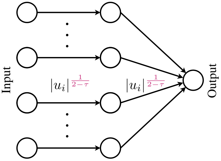
Figure 2: A reparameterized linear neuron where wi=|ui|22−τw_{i}=|u_{i}|^{\frac{2}{2-\tau}} as a two-layer sparse network: value of τ=0\tau=0 reduces to GD while τ=1\tau=1 simulates the EGU update.

An equivalent integral version of this update is

𝒘⁡(t)=expτ⁡(logτ⁡𝒘0−η​∫0t∇𝒘L​(𝒘⁡(z))​𝑑z),{\bm{w}}(t)=\exp_{\tau}\!\big(\log_{\tau}{\bm{w}}_{0}-\eta\,\int_{0}^{t}\!\!\nabla_{{\bm{w}}}L({\bm{w}}(z))\,\mathrm{d}z\big), (22)

where expτ⁡(x)≔[1+(1−τ)​x]+11−τ\exp_{\tau}(x)\coloneqq[1+(1-\tau)x]_{+}^{\frac{1}{1-\tau}} is the inverse of tempered logarithm (19). Note that τ=1\tau=1 is a limit case which recovers the standard exp\exp function and the update (21) becomes the standard EGU update. Additionally, the GD update (on the non-negative orthant) is recovered at τ=0\tau=0. As a result, the tempered EGU update (21) interpolates between GD and EGU for τ∈[0,1]\tau\in[0,1] and generalize beyond for values of τ>1\tau>1 and τ<0\tau<0.66 6 For example, τ=2\tau=2 corresponds to the Burg updates (Example 4). We now show the reparameterization of the tempered EGU update (21) as GD. This corresponds to continuous-time gradient descent on the network of Figure 2.

Proposition 2.

The tempered continuous EGU update can be reparameterized continuous-time GD with the reparameterization function

𝒘=qτ(𝒖)=(2−τ2)22−τ|𝒖|⊙22−τ,for 𝒖∈ℝd and τ≠2.{\bm{w}}=q_{\tau}(\bm{u})=\big(\frac{2-\tau}{2}\big)^{\frac{2}{2-\tau}}|\bm{u}|^{\odot\frac{2}{2-\tau}}\,,\,\,\text{for }\bm{u}\in\mathbb{R}^{d}\text{ and }\tau\neq 2\,. (23)

That is

logτ∙τ(𝒘)=−η∇\displaystyle{\stackrel{{\scriptstyle\scriptscriptstyle\mathbin{\vbox{\hbox{\scalebox{0.42}{$\bullet$}}}}}}{{\log_{\tau}}}}({\bm{w}})=-\eta\nabla L(𝒘)equals𝒖∙=−η∇L∘qτ​(𝒖)⏟∇𝒖L​((2−τ2)22−τ​|𝒖|⊙22−τ)=−ηsign(𝒖)⊙(2−τ2)τ2−τ|𝒖|⊙τ2−τ⊙∇L(𝒘).\displaystyle\!L({\bm{w}})\;\text{equals}\;{\stackrel{{\scriptstyle\scriptscriptstyle\mathbin{\vbox{\hbox{\scalebox{0.42}{$\bullet$}}}}}}{{\bm{u}}}}=-\eta\!\!\!\!\!\!\!\!\!\!\!\!\!\!\!\underbrace{\nabla L\!\circ\!q_{\tau}\,(\bm{u})}_{\nabla_{\bm{u}}L\big(\big(\frac{2-\tau}{2}\big)^{\frac{2}{2-\tau}}|\bm{u}|^{{\odot\frac{2}{2-\tau}}}\big)}\!\!\!\!\!\!\!\!\!\!\!\!\!\!\!={-\eta\sign(\bm{u})\!\odot\!\Big(\frac{2-\tau}{2}\Big)^{\frac{\tau}{2-\tau}}\!|\bm{u}|^{\odot\frac{\tau}{2-\tau}}\!\odot\!\nabla L({\bm{w}})}.
Proof.

This is verified by checking the condition of Theorem 2. The lhs is

(𝑯Fτ​(𝒘)​(𝒘))−1=(𝑱logτ​(𝒘))−1\displaystyle{(\bm{H}_{F_{\tau}({\bm{w}})}({\bm{w}}))^{-1}=(\bm{J}_{\log_{\tau}}({\bm{w}}))^{-1}} =(diag⁡(𝒘)−τ)−1=diag⁡(𝒘)τ.\displaystyle{=(\diag({\bm{w}})^{-\tau})^{-1}=\diag({\bm{w}})^{\tau}}.

Note that the Jacobian of qτq_{\tau} is

𝑱qτ​(𝒖)=(2−τ2)τ2−τ​diag⁡(sign⁡(𝒖)⊙|𝒖|⊙τ2−τ)=diag⁡(sign⁡(𝒖)⊙qτ​(𝒖)⊙τ2).\bm{J}_{\!q_{\tau}}(\bm{u})=\Big(\frac{2-\tau}{2}\Big)^{\frac{\tau}{2-\tau}}\diag\big(\sign(\bm{u})\odot|\bm{u}|^{\odot\frac{\tau}{2-\tau}}\big)=\diag(\sign(\bm{u})\odot q_{\tau}(\bm{u})^{\odot\frac{\tau}{2}}).

Thus the rhs 𝑱qτ​(𝒖)​𝑱qτ⊤​(𝒖)\bm{J}_{\!q_{\tau}}(\bm{u})\bm{J}_{\!q_{\tau}}^{\top}(\bm{u}) of the condition equals diag⁡(𝒘⊙τ)\diag\big({\bm{w}}^{\odot\tau}\big) as well. ∎

4.2 Minimum-norm Solutions

We apply the (reparameterized) tempered EGU update on the under-determined linear regression problem. For this, we first consider the ±\pm-trick on (21), in which we set 𝒘⁡(t)=𝒘+​(t)−𝒘−​(t){\bm{w}}(t)={\bm{w}}_{+}(t)-{\bm{w}}_{-}(t) where

logτ∙τ𝒘+(t)=−η∇𝒘L(𝒘(t)),logτ∙τ𝒘−(t)=+η∇𝒘L(𝒘(t)).{\stackrel{{\scriptstyle\scriptscriptstyle\mathbin{\vbox{\hbox{\scalebox{0.42}{$\bullet$}}}}}}{{\log_{\tau}}}}{\bm{w}}_{+}(t)=-\eta\,\nabla_{{\bm{w}}}L({\bm{w}}(t))\,,\quad{\stackrel{{\scriptstyle\scriptscriptstyle\mathbin{\vbox{\hbox{\scalebox{0.42}{$\bullet$}}}}}}{{\log_{\tau}}}}{\bm{w}}_{-}(t)=+\eta\,\nabla_{{\bm{w}}}L({\bm{w}}(t))\,. (24)

Note that using the ±\pm-trick, we have 𝒘⁡(t)∈ℝn{\bm{w}}(t)\in\mathbb{R}^{n}. We call the updates (24) the tempered EGU±. The reparameterization of the tempered EGU± updates as GD can be written by applying Proposition 2,

𝒖∙+(t)=−η∇𝒖+L(qτ(𝒖+(t))−qτ(𝒖−(t))),𝒖∙−(t)=−η∇𝒖−L(qτ(𝒖+(t))−qτ(𝒖−(t))),{\stackrel{{\scriptstyle\scriptscriptstyle\mathbin{\vbox{\hbox{\scalebox{0.42}{$\bullet$}}}}}}{{\bm{u}}}}_{+}\!(t)=-\eta\,\nabla_{\bm{u}_{+}}L\big(q_{\tau}(\bm{u}_{+}(t))-q_{\tau}(\bm{u}_{-}(t))\big)\,,{\stackrel{{\scriptstyle\scriptscriptstyle\mathbin{\vbox{\hbox{\scalebox{0.42}{$\bullet$}}}}}}{{\bm{u}}}}_{-}\!(t)=-\eta\,\nabla_{\bm{u}_{-}}L\big(q_{\tau}(\bm{u}_{+}(t))-q_{\tau}(\bm{u}_{-}(t))\big), (25)

and setting 𝒘⁡(t)=qτ​(𝒖+​(t))−qτ​(𝒖−​(t)){\bm{w}}(t)=q_{\tau}(\bm{u}_{+}(t))-q_{\tau}(\bm{u}_{-}(t)).

The strong convexity of the FτF_{\tau} function w.r.t. the L2−τ\mathrm{L}_{2-\tau}-norm (see (Amid et al. 2019)) suggests that the updates motivated by the tempered Bregman divergence (4) yield the minimum L2−τ\mathrm{L}_{2-\tau}-norm solution in certain settings. We verify this by considering the following under-determined linear regression problem. Let {𝒙n,yn}n=1N\{\bm{x}_{n},y_{n}\}_{n=1}^{N} where 𝒙n∈ℝd,yn∈ℝ\bm{x}_{n}\in\mathbb{R}^{d},\,y_{n}\in\mathbb{R} denote the set of input-output pairs and let 𝑿∈ℝN×d\bm{X}\in\mathbb{R}^{N\times d} be the design matrix for which the nn-th row is equal to 𝒙n⊤\bm{x}_{n}^{\top}. Also, let 𝒚∈ℝN\bm{y}\in\mathbb{R}^{N} denote the vector of targets. Consider the tempered EGU± updates (24) on the weights 𝒘⁡(t)=𝒘+​(t)−𝒘−​(t){\bm{w}}(t)={\bm{w}}_{+}(t)-{\bm{w}}_{-}(t) where 𝒘+​(t),𝒘−​(t)≥𝟎{\bm{w}}_{+}(t),{\bm{w}}_{-}(t)\geq\bm{0} and 𝒘+​(0)=𝒘−​(0)=𝒘0{\bm{w}}_{+}(0)={\bm{w}}_{-}(0)={\bm{w}}_{0}. Following (22), we have

𝒘+​(t)=expτ⁡(logτ⁡𝒘0−η​∫0t𝑿⊤​𝜹​(z)​𝑑z),𝒘−​(t)=expτ⁡(logτ⁡𝒘0+η​∫0t𝑿⊤​𝜹​(z)​𝑑z),{\bm{w}}_{+}(t)=\exp_{\tau}\big(\log_{\tau}{\bm{w}}_{0}-\eta\,\int_{0}^{t}\bm{X}^{\top}\bm{\delta}(z)\,\mathrm{d}z\big)\,,\,\,{\bm{w}}_{-}(t)=\exp_{\tau}\big(\log_{\tau}{\bm{w}}_{0}+\eta\,\int_{0}^{t}\bm{X}^{\top}\bm{\delta}(z)\,\mathrm{d}z\big)\,,

where 𝜹⁡(t)=𝑿⁡(𝒘+​(t)−𝒘−​(t))\bm{\delta}(t)=\bm{X}\big({\bm{w}}_{+}(t)-{\bm{w}}_{-}(t)\big) .

Theorem 4.

Consider the underdetermined linear regression problem where N<dN<d. Let ℰ={𝐰∈ℝd|𝐗​𝐰=𝐲}\mathcal{E}=\{{\bm{w}}\in\mathbb{R}^{d}|\,\bm{X}{\bm{w}}=\bm{y}\} be the set of solutions with zero error. Given 𝐰⁡(∞)∈ℰ{\bm{w}}(\infty)\in\mathcal{E}, then the tempered EGU± updates (24) with temperature 0≤τ≤10\leq\tau\leq 1 and initial solution 𝐰0=α​𝟏≥0{\bm{w}}_{0}=\alpha\bm{1}\geq 0 converge to the minimum L2−τ\mathrm{L}_{2-\tau}-norm solution in ℰ\mathcal{E} in the limit α→0\alpha\rightarrow 0.

Proof.

We show that the solution of the tempered EGU± satisfies the dual feasibility and complementary slackness KKT conditions for the following optimization problem (omitting tt for simplicity):

min𝒘+,𝒘−⁡‖𝒘+−𝒘−‖2−τ2−τ,for ​0≤τ≤1,s.t.𝑿⁡(𝒘+−𝒘−)=𝒚​ and ​𝒘+,𝒘−≥𝟎.\displaystyle\quad\min_{{\bm{w}}_{+},{\bm{w}}_{-}}\,\|{\bm{w}}_{+}-{\bm{w}}_{-}\|_{2-\tau}^{2-\tau},\,\,\,\text{for }0\leq\tau\leq 1,\quad\text{s.t.}\quad\bm{X}({\bm{w}}_{+}-{\bm{w}}_{-})=\bm{y}\,\,\,\text{ and }\,\,\,{\bm{w}}_{+},{\bm{w}}_{-}\geq\bm{0}\,.

Imposing the constraints using a set of Lagrange multipliers 𝝂+,𝝂−≥𝟎\bm{\nu}_{+},\bm{\nu}_{-}\geq\bm{0} and λ∈ℝ\lambda\in\mathbb{R}, we have

min⁡sup𝝂+,𝝂−≥𝟎,λ𝒘⁡{‖𝒘+−𝒘−‖2−τ2−τ+𝝀⊤​(𝑿⁡(𝒘+−𝒘−)−𝒚)−𝒘+⊤​𝝂+−𝒘−⊤​𝝂−}.\min_{\bm{w}}\sup_{\bm{\nu}_{+},\bm{\nu}_{-}\geq\bm{0},\lambda}\,\,\Big\{\|{\bm{w}}_{+}-{\bm{w}}_{-}\|^{2-\tau}_{2-\tau}+\bm{\lambda}^{\top}\,\big(\bm{X}({\bm{w}}_{+}-{\bm{w}}_{-})-\bm{y}\big)-{\bm{w}}_{+}^{\top}\bm{\nu}_{+}-{\bm{w}}_{-}^{\top}\bm{\nu}_{-}\Big\}\,.

The set of KKT conditions are

{𝒘+,𝒘−≥𝟎,𝑿​𝒘=𝒚,+sign(𝒘)⊙|𝒘|⊙(1−τ)−𝑿⊤𝝀≽𝟎,−sign(𝒘)⊙|𝒘|⊙(1−τ)+𝑿⊤𝝀≽𝟎,(sign(𝒘)⊙|𝒘|⊙(1−τ)−𝑿⊤𝝀)⊙𝒘+=𝟎,(sign(𝒘)⊙|𝒘|⊙(1−τ)−𝑿⊤𝝀)⊙𝒘−=𝟎,\begin{cases}{\bm{w}}_{+},{\bm{w}}_{-}\geq\bm{0}\,,\,\,\bm{X}{\bm{w}}=\bm{y}\,,\\ +\sign({\bm{w}})\odot|{\bm{w}}|^{\odot(1-\tau)}-\bm{X}^{\top}\bm{\lambda}\succcurlyeq\bm{0}\,,\,\,-\sign({\bm{w}})\odot|{\bm{w}}|^{\odot(1-\tau)}+\bm{X}^{\top}\bm{\lambda}\succcurlyeq\bm{0}\,,\\ \big(\sign({\bm{w}})\odot|{\bm{w}}|^{\odot(1-\tau)}-\bm{X}^{\top}\bm{\lambda}\big)\odot{\bm{w}}_{+}=\bm{0}\,,\,\,\big(\sign({\bm{w}})\odot|{\bm{w}}|^{\odot(1-\tau)}-\bm{X}^{\top}\bm{\lambda}\big)\odot{\bm{w}}_{-}=\bm{0}\,,\end{cases}

where 𝒘=𝒘+−𝒘−{\bm{w}}={\bm{w}}_{+}-{\bm{w}}_{-}. The first condition is imposed by the form of the updates and the second condition is satisfied by the assumption at t→∞t\rightarrow\infty. Using 𝒘0=α​𝟏{\bm{w}}_{0}=\alpha\bm{1} with α→0\alpha\rightarrow 0, we have

𝒘+​(t)\displaystyle{\bm{w}}_{+}(t) =expτ(−11−τ−η∫0t𝑿⊤𝜹(z)dz)=[−(1−τ)η𝑿∫0t𝜹(z)]+⊙11−τ,\displaystyle=\exp_{\tau}\big(-\frac{1}{1-\tau}-\eta\,\int_{0}^{t}\bm{X}^{\top}\bm{\delta}(z)\,\mathrm{d}z\big)=\big[-(1-\tau)\,\eta\,\bm{X}\int_{0}^{t}\bm{\delta}(z)\big]_{+}^{\odot\frac{1}{1-\tau}}\,,
𝒘−​(t)\displaystyle{\bm{w}}_{-}(t) =expτ(−11−τ+η∫0t𝑿⊤𝜹(z)dz)=[+(1−τ)η𝑿∫0t𝜹(z)]+⊙11−τ.\displaystyle=\exp_{\tau}\big(-\frac{1}{1-\tau}+\eta\,\int_{0}^{t}\bm{X}^{\top}\bm{\delta}(z)\,\mathrm{d}z\big)=\big[+(1-\tau)\,\eta\,\bm{X}\int_{0}^{t}\bm{\delta}(z)\big]_{+}^{\odot\frac{1}{1-\tau}}\,.

Setting 𝝀=−(1−τ)η∫0∞𝜹(z)\bm{\lambda}=-(1-\tau)\,\eta\int_{0}^{\infty}\bm{\delta}(z) satisfies the remaining KKT conditions. ∎

Corollary 1.

Under the assumptions of Theorem 4, the reparameterized tempered EGU± updates (25) also recover the minimum L2−τ\mathrm{L}_{2-\tau}-norm solution where 𝐰⁡(t)=qτ​(𝐮+​(t))−qτ​(𝐮−​(t)){\bm{w}}(t)=q_{\tau}(\bm{u}_{+}(t))-q_{\tau}(\bm{u}_{-}(t)).

This corollary shows that reparameterizing the loss in terms of the parameters 𝒖\bm{u} changes the implicit bias of the GD updates. Similar results were observed before in terms of sparse signal recovery (Vaskevicius et al. 2019) and matrix factorization (Gunasekar et al. 2017). Here, we show that this is a direct result of the dynamics induced by the reparameterization Theorem 2.

5 Conclusion and Future Work

In this paper, we discussed the continuous-time mirror descent updates and provided a general framework for reparameterizing these updates. Additionally, we introduced the tempered EGU± updates and their reparameterized forms. The tempered EGU± updates include the two commonly used gradient descent and exponentiated gradient updates, and interpolations between them. For the underdetermined linear regression problem we showed that under certain conditions, the tempered EGU± updates converge to the minimum L2−τ\mathrm{L}_{2-\tau}-norm solution. The current work leads to many interesting future directions:

  • •

    The focus is this paper was to develop the reparameterization method in full generality. Our reparameterization equivalence theorem holds only in the continuous-time and the equivalence relation breaks down after discretization. However, in many important cases the discretized reparameterized updates closely track the discretized original updates (Amid and Warmuth 2020). This was done by proving the same on-line worst case regret bounds for the discretized reparameterized updates and the originals. A key research direction is to find general conditions for which this is true.

  • •

    Perhaps the most important application of the current work is reparameterizing the weights of deep neural networks for achieving sparse solutions or obtaining an implicit form of regularization that mimics a trade-off between the ridge and lasso methods (e.g. elastic net regularization (Zou and Hastie 2005)). Here the deep open question is the following: Are sparse networks (as in Figure 2) required, if the goal is to obtain sparse solutions efficiently?

  • •

    A more general treatment of the underdetermined linear regression case requires analyzing the results for arbitrary start vectors. Also, developing a matrix form of the reparameterization theorem is left for future work.

Broader Impact

The result of the paper suggests that the mirror descent updates can be effectively used in neural networks by running backpropagation on the reparameterized form of the neurons. This may have a potential use case for training these networks more efficiently. This is a theoretical paper and the broader ethical impact discussion is not applicable.

References

  • Akin [1979] Ethan Akin. The geometry of population genetics, volume 31 of Lecture Notes in Biomathematics. Springer-Verlag, Berlin-New York, 1979.
  • Amari [1998] Shun-ichi Amari. Natural gradient works efficiently in learning. Neural Computation, 10(2):251–276, 1998.
  • Amid et al. [2019] E. Amid, M. K. Warmuth, R. Anil, and K. Tomer. Robust bi-tempered logistic loss based on Bregman divergences. In Proceedings of the 32nd International Conference on Neural Information Processing Systems, NeurIPS’19, Cambridge, MA, USA, 2019.
  • Amid and Warmuth [2020] Ehsan Amid and Manfred K. Warmuth. Winnowing with gradient descent. In Conference on Learning Theory (COLT), 2020.
  • Burke [1985] William L. Burke. Applied Differential Geometry. Cambridge University Press, 1985.
  • Cesa-Bianchi et al. [2007] Nicolo Cesa-Bianchi, Yishay Mansour, and Gilles Stoltz. Improved second-order bounds for prediction with expert advice. Machine Learning, 66(2-3):321–352, 2007.
  • Cichocki and Amari [2010] Andrzej Cichocki and Shun-ichi Amari. Families of alpha-beta-and gamma-divergences: Flexible and robust measures of similarities. Entropy, 12(6):1532–1568, 2010.
  • Ghai et al. [2019] U. Ghai, E. Hazan, and S. Singer. Exponentiated gradient vs. meets gradient descent. arXiv preprint arXiv:1902.01903, 2019.
  • Gunasekar et al. [2017] Suriya Gunasekar, Blake E Woodworth, Srinadh Bhojanapalli, Behnam Neyshabur, and Nati Srebro. Implicit regularization in matrix factorization. In Advances in Neural Information Processing Systems (NeurIPS), pages 6151–6159, 2017.
  • Gunasekar et al. [2018] Suriya Gunasekar, Jason D Lee, Daniel Soudry, and Nati Srebro. Implicit bias of gradient descent on linear convolutional networks. In Advances in Neural Information Processing Systems (NeurIPS), pages 9461–9471, 2018.
  • Kivinen et al. [1997] J. Kivinen, M. K. Warmuth, and P. Auer. The Perceptron algorithm vs. Winnow: linear vs. logarithmic mistake bounds when few input variables are relevant. Artificial Intelligence, 97:325–343, December 1997.
  • Kivinen and Warmuth [1997] Jyrki Kivinen and Manfred K. Warmuth. Exponentiated gradient versus gradient descent for linear predictors. Information and Computation, 132(1):1–63, 1997.
  • Kivinen et al. [2006] Jyrki Kivinen, Manfred K Warmuth, and Babak Hassibi. The p-norm generalization of the LMS algorithm for adaptive filtering. IEEE Transactions on Signal Processing, 54(5):1782–1793, 2006.
  • Littlestone and Warmuth [1994] N Littlestone and MK Warmuth. The weighted majority algorithm. Information and Computation, 108(2):212–261, 1994.
  • Naudts [2002] Jan Naudts. deformed exponentials and logarithms in generalized thermostatistics. physica a, 316:323–334, 2002. URL http://arxiv.org/pdf/cond-mat/0203489.
  • Nemirovsky and Yudin [1983] A. Nemirovsky and D. Yudin. Problem Complexity and Method Efficiency in Optimization. Wiley & Sons, New York, 1983.
  • Nie et al. [2016] Jiazhong Nie, Wojciech Kotłowski, and Manfred K Warmuth. Online PCA with optimal regret. The Journal of Machine Learning Research, 17(1):6022–6070, 2016.
  • Raginsky and Bouvrie [2012] Maxim Raginsky and Jake Bouvrie. Continuous-time stochastic mirror descent on a network: Variance reduction, consensus, convergence. In 2012 IEEE 51st IEEE Conference on Decision and Control (CDC), pages 6793–6800. IEEE, 2012.
  • Raskutti and Mukherjee [2015] Garvesh Raskutti and Sayan Mukherjee. The information geometry of mirror descent. IEEE Transactions on Information Theory, 61(3):1451–1457, 2015.
  • Rockafellar [1976] R Tyrrell Rockafellar. Monotone operators and the proximal point algorithm. SIAM journal on control and optimization, 14(5):877–898, 1976.
  • Sandholm [2010] William H Sandholm. Population games and evolutionary dynamics. MIT Press, 2010.
  • Shalev-Shwartz et al. [2012] Shai Shalev-Shwartz et al. Online learning and online convex optimization. Foundations and Trends® in Machine Learning, 4(2):107–194, 2012.
  • Vaskevicius et al. [2019] Tomas Vaskevicius, Varun Kanade, and Patrick Rebeschini. Implicit regularization for optimal sparse recovery. In Advances in Neural Information Processing Systems (NeurIPS), pages 2968–2979, 2019.
  • Vishwanathan and Warmuth [2005] S.V.N. Vishwanathan and M.K. Warmuth. Leaving the span. In Proceedings of the 18th Annual Conference on Learning Theory (COLT), 2005.
  • Warmuth and Jagota [1998] M. K. Warmuth and A. Jagota. Continuous and discrete time nonlinear gradient descent: relative loss bounds and convergence. In R. Greiner E. Boros, editor, Electronic Proceedings of Fifth International Symposium on Artificial Intelligence and Mathematics. Electronic,http://rutcor.rutgers.edu/~\tilde{\penalty\ }amai, 1998.
  • Warmuth et al. [2014] M. K. Warmuth, W. Kotłowski, and S. Zhou. Kernelization of matrix updates. Journal of Theoretical Computer Science, 558:159–178, 2014. Special issue for the 23nd International Conference on Algorithmic Learning Theory (ALT’12).
  • Zou and Hastie [2005] Hui Zou and Trevor Hastie. Regularization and variable selection via the elastic net. Journal of the royal statistical society: series B (statistical methodology), 67(2):301–320, 2005.

Appendix A Dual Form of Bregman Momentum

The dual form of Bregman momentum given in (12) can be obtained by first forming the dual Bregman divergence in terms of the dual variables 𝒘∗​(t){\bm{w}}^{*}(t) and 𝒘s∗{\bm{w}}_{s}^{*} and taking the time derivative, that is,

D∙F(𝒘(t),𝒘0)\displaystyle{\stackrel{{\scriptstyle\scriptscriptstyle\mathbin{\vbox{\hbox{\scalebox{0.42}{$\bullet$}}}}}}{{D}}}_{F}({\bm{w}}(t),{\bm{w}}_{0}) =D∙F∗(𝒘0∗,𝒘∗(t))=∂∂t(F∗(𝒘0∗)−F∗(𝒘∗(t))−f∗(𝒘∗(t))⊤(𝒘0∗−𝒘∗(t))\displaystyle={\stackrel{{\scriptstyle\scriptscriptstyle\mathbin{\vbox{\hbox{\scalebox{0.42}{$\bullet$}}}}}}{{D}}}_{F^{*}}({\bm{w}}_{0}^{*},{\bm{w}}^{*}(t))=\frac{\partial}{\partial t}\Big(F^{*}({\bm{w}}_{0}^{*})-F^{*}({\bm{w}}^{*}(t))-f^{*}({\bm{w}}^{*}(t))^{\top}\big({\bm{w}}_{0}^{*}-{\bm{w}}^{*}(t)\big)
=−F∗∙∗(𝒘∗(t))+f∗(𝒘∗(t))⊤∙𝒘∗(t)+(𝒘∗(t)−𝒘0∗)⊤𝑯F∗(𝒘∗(t))∙𝒘∗(t)\displaystyle=-{\stackrel{{\scriptstyle\scriptscriptstyle\mathbin{\vbox{\hbox{\scalebox{0.42}{$\bullet$}}}}}}{{F^{*}}}}({\bm{w}}^{*}(t))+f^{*}({\bm{w}}^{*}(t))^{\top}\mathrel{\vbox{\halign{\hfil#\hfil\cr$\scriptscriptstyle\mathbin{\vbox{\hbox{\scalebox{0.4}{$\bullet$}}}}$\cr\kern 1.72218pt\cr${\bm{w}}$\cr}}}^{*}\!\!(t)+({\bm{w}}^{*}(t)-{\bm{w}}_{0}^{*})^{\top}\bm{H}_{F^{*}}({\bm{w}}^{*}(t))\,\mathrel{\vbox{\halign{\hfil#\hfil\cr$\scriptscriptstyle\mathbin{\vbox{\hbox{\scalebox{0.4}{$\bullet$}}}}$\cr\kern 1.72218pt\cr${\bm{w}}$\cr}}}^{*}\!\!(t)
=(𝒘∗(t)−𝒘0∗)⊤𝑯F∗(𝒘∗(t))∙𝒘∗(t),\displaystyle=\big({\bm{w}}^{*}(t)-{\bm{w}}_{0}^{*}\big)^{\top}\bm{H}_{F^{*}}({\bm{w}}^{*}(t))\,\mathrel{\vbox{\halign{\hfil#\hfil\cr$\scriptscriptstyle\mathbin{\vbox{\hbox{\scalebox{0.4}{$\bullet$}}}}$\cr\kern 1.72218pt\cr${\bm{w}}$\cr}}}^{*}\!\!(t)\,,

where we use the fact that F∗∙∗(𝒘∗(t))=f∗(𝒘∗(t))⊤∙𝒘∗(t){\stackrel{{\scriptstyle\scriptscriptstyle\mathbin{\vbox{\hbox{\scalebox{0.42}{$\bullet$}}}}}}{{F^{*}}}}({\bm{w}}^{*}(t))=f^{*}({\bm{w}}^{*}(t))^{\top}\mathrel{\vbox{\halign{\hfil#\hfil\cr$\scriptscriptstyle\mathbin{\vbox{\hbox{\scalebox{0.4}{$\bullet$}}}}$\cr\kern 1.72218pt\cr${\bm{w}}$\cr}}}^{*}\!\!(t).

Appendix B Constrained Updates and Reparameterization

We first provide a proof for Proposition 1. Then, we prove Theorem 3.

Proposition 1.  The CMD update with the additional constraint ψ⁡(𝐰⁡(t))=𝟎\psi\big({\bm{w}}(t)\big)=\bm{0}  for some function ψ:ℝd→ℝm\psi:\,\mathbb{R}^{d}\rightarrow\mathbb{R}^{m} s.t. {𝐰∈𝒞|ψ⁡(𝐰⁡(t))=𝟎}\{{\bm{w}}\in\mathcal{C}|\,\psi\big({\bm{w}}(t)\big)=\bm{0}\} is non-empty, amounts to the projected gradient update

f∙(𝒘(t))=−η𝑷ψ(𝒘(t))∇L(𝒘(t))&f∗∙∗(𝒘∗(t))=−η𝑷ψ(𝒘(t))⊤∇L∘f∗(𝒘∗(t)),{\stackrel{{\scriptstyle\scriptscriptstyle\mathbin{\vbox{\hbox{\scalebox{0.42}{$\bullet$}}}}}}{{f}}}\big({\bm{w}}(t)\big)=-\eta\,\bm{P}_{\psi}({\bm{w}}(t))\nabla L({\bm{w}}(t))\;\&\;{\stackrel{{\scriptstyle\scriptscriptstyle\mathbin{\vbox{\hbox{\scalebox{0.42}{$\bullet$}}}}}}{{f^{*}}}}({\bm{w}}^{*}(t))=-\eta\,\bm{P}_{\psi}({\bm{w}}(t))^{\top}\,\nabla L\!\circ\!f^{*}\,({\bm{w}}^{*}(t))\,, (17)

where 𝐏ψ≔𝐈d−𝐉ψ⊤​(𝐉ψ​𝐇F−1​𝐉ψ⊤)−1​𝐉ψ​𝐇F−1\bm{P}_{\psi}\coloneqq\bm{I}_{d}-\bm{J}^{\top}_{\psi}\big(\bm{J}_{\psi}\bm{H}^{-1}_{F}\bm{J}^{\top}_{\psi}\big)^{-1}\bm{J}_{\psi}\bm{H}^{-1}_{F} is the projection matrix onto the tangent space of FF\; at 𝐰⁡(t){\bm{w}}(t) and 𝐉ψ​(𝐰​(t))\bm{J}_{\psi}({\bm{w}}(t)). Equivalently, the update can be written as a projected natural gradient descent update

𝒘∙(t)=−η𝑷ψ⊤(𝒘(t))𝑯F−1(𝒘(t))∇L(𝒘(t))&∙𝒘∗(t)=−η𝑷ψ𝑯F∗−1(𝒘∗(t))∇L∘f∗(𝒘∗(t)).{\stackrel{{\scriptstyle\scriptscriptstyle\mathbin{\vbox{\hbox{\scalebox{0.42}{$\bullet$}}}}}}{{{\bm{w}}}}}(t)\!=\!-\eta\bm{P}^{\top}_{\psi}({\bm{w}}(t))\bm{H}_{F}^{-1}({\bm{w}}(t))\nabla L({\bm{w}}(t))\,\&\,\mathrel{\vbox{\halign{\hfil#\hfil\cr$\scriptscriptstyle\mathbin{\vbox{\hbox{\scalebox{0.4}{$\bullet$}}}}$\cr\kern 1.72218pt\cr${\bm{w}}$\cr}}}^{*}\!\!(t)\!=\!-\eta\bm{P}_{\psi}\bm{H}_{F^{*}}^{-1}({\bm{w}}^{*}(t))\nabla L\!\circ\!f^{*}({\bm{w}}^{*}(t)).\!\!\! (18)
Proof of Proposition 1.

We use a Lagrange multiplier 𝝀⁡(t)∈ℝm\bm{\lambda}(t)\in\mathbb{R}^{m} in (6) to enforce the constraint ψ⁡(𝒘⁡(t))=𝟎\psi({\bm{w}}(t))=\bm{0} for all t≥0t\geq 0,

min𝒘⁡(t){1/ηD∙F(𝒘(t),𝒘s)+L(𝒘(t))+𝝀(t)⊤ψ(𝒘(t))}.\displaystyle\min_{{\bm{w}}(t)}\,\Big\{\nicefrac{{1}}{{\eta}}\,{\stackrel{{\scriptstyle\scriptscriptstyle\mathbin{\vbox{\hbox{\scalebox{0.42}{$\bullet$}}}}}}{{D}}}_{F}({\bm{w}}(t),{\bm{w}}_{s})+L({\bm{w}}(t))+\bm{\lambda}(t)^{\top}\psi({\bm{w}}(t))\Big\}\,. (26)

Setting the derivative w.r.t. 𝒘⁡(t){\bm{w}}(t) to zero, we have

f∙(𝒘⁡(t))+η​∇𝒘L​(𝒘⁡(t))+𝑱ψ​(𝒘⁡(t))⊤​𝝀​(t)=𝟎,{\stackrel{{\scriptstyle\scriptscriptstyle\mathbin{\vbox{\hbox{\scalebox{0.42}{$\bullet$}}}}}}{{f}}}({\bm{w}}(t))+\eta\,\nabla_{{\bm{w}}}L({\bm{w}}(t))+\bm{J}_{\psi}({\bm{w}}(t))^{\top}\bm{\lambda}(t)=\bm{0}\,, (27)

where 𝑱ψ​(𝒘​(t))\bm{J}_{\psi}({\bm{w}}(t)) is the Jacobian of the function ψ⁡(𝒘⁡(t))\psi({\bm{w}}(t)). In order to solve for 𝝀⁡(t)\bm{\lambda}(t), first note that ψ∙(𝒘⁡(t))=𝑱ψ​(𝒘⁡(t))𝒘∙(t)=𝟎{\stackrel{{\scriptstyle\scriptscriptstyle\mathbin{\vbox{\hbox{\scalebox{0.42}{$\bullet$}}}}}}{{\psi}}}({\bm{w}}(t))=\bm{J}_{\psi}({\bm{w}}(t))\,{\stackrel{{\scriptstyle\scriptscriptstyle\mathbin{\vbox{\hbox{\scalebox{0.42}{$\bullet$}}}}}}{{{\bm{w}}}}}(t)=\bm{0}. Using the equality f∙(𝒘⁡(t))=𝑯F​(𝒘⁡(t))𝒘∙(t){\stackrel{{\scriptstyle\scriptscriptstyle\mathbin{\vbox{\hbox{\scalebox{0.42}{$\bullet$}}}}}}{{f}}}({\bm{w}}(t))=\bm{H}_{F}({\bm{w}}(t)){\stackrel{{\scriptstyle\scriptscriptstyle\mathbin{\vbox{\hbox{\scalebox{0.42}{$\bullet$}}}}}}{{{\bm{w}}}}}(t) and multiplying both sides by 𝑱ψ​(𝒘⁡(t))​𝑯F−1​(𝒘⁡(t))\bm{J}_{\psi}({\bm{w}}(t))\bm{H}^{-1}_{F}({\bm{w}}(t)) yields (ignoring tt)

J_ψ(w)    w     ∙     +η𝑱ψ(𝒘)𝑯F−1(𝒘)∇L(𝒘)+𝑱ψ(𝒘)𝑯F−1(𝒘)𝑱ψ⊤(𝒘)𝝀(t)=𝟎\displaystyle\cancel{\bm{J}_\psi({\bm{w}})\, {\stackrel{{\scriptstyle\scriptscriptstyle\mathbin{\vbox{\hbox{\scalebox{0.42}{$\bullet$}}}}}}{{{\bm{w}}}}} }+\eta\,\bm{J}_{\psi}({\bm{w}})\bm{H}^{-1}_{F}({\bm{w}})\nabla L({\bm{w}})+\bm{J}_{\psi}({\bm{w}})\bm{H}^{-1}_{F}({\bm{w}})\bm{J}^{\top}_{\psi}({\bm{w}})\bm{\lambda}(t)=\bm{0}

Assuming that the inverse exists, we can written

𝝀=−η(𝑱ψ(𝒘)𝑯F−1(𝒘)𝑱ψ⊤(𝒘))−1𝑱ψ(𝒘)𝑯F−1(𝒘)∇L(𝒘).\displaystyle\bm{\lambda}=-\eta\,\big(\bm{J}_{\psi}({\bm{w}})\bm{H}^{-1}_{F}({\bm{w}})\bm{J}^{\top}_{\psi}({\bm{w}})\big)^{-1}\bm{J}_{\psi}({\bm{w}})\bm{H}^{-1}_{F}({\bm{w}})\nabla L({\bm{w}})\,.

Plugging in for 𝝀⁡(t)\bm{\lambda}(t) yields (18). Multiplying both sides by 𝑯F​(𝒘)\bm{H}_{F}({\bm{w}}) and using f∙(𝒘)=𝑯F​(𝒘)𝒘∙{\stackrel{{\scriptstyle\scriptscriptstyle\mathbin{\vbox{\hbox{\scalebox{0.42}{$\bullet$}}}}}}{{f}}}({\bm{w}})=\bm{H}_{F}({\bm{w}}){\stackrel{{\scriptstyle\scriptscriptstyle\mathbin{\vbox{\hbox{\scalebox{0.42}{$\bullet$}}}}}}{{{\bm{w}}}}} yields (17). ∎

Theorem 3. The constrained CMD update (17) coincides with the reparameterized projected gradient update on the composite loss,

g∙(𝒖(t))=−η𝑷ψ∘q(𝒖(t))∇𝒖L∘q(𝒖(t)),{\stackrel{{\scriptstyle\scriptscriptstyle\mathbin{\vbox{\hbox{\scalebox{0.42}{$\bullet$}}}}}}{{g}}}\big(\bm{u}(t)\big)=-\eta\,\bm{P}_{\psi\circ q}(\bm{u}(t))\nabla_{\bm{u}}L\circ q(\bm{u}(t))\,,

where 𝐏ψ∘q≔𝐈k−𝐉ψ∘q⊤​(𝐉ψ∘q​𝐇G−1​𝐉ψ∘q⊤)−1​𝐉ψ∘q​𝐇G−1\bm{P}_{\psi\circ q}\coloneqq\bm{I}_{k}-\bm{J}^{\top}_{\psi\circ q}\big(\bm{J}_{\psi\circ q}\bm{H}^{-1}_{G}\bm{J}^{\top}_{\psi\circ q}\big)^{-1}\bm{J}_{\psi\circ q}\bm{H}^{-1}_{G} is the projection matrix onto the tangent space at 𝐮⁡(t)\bm{u}(t) and 𝐉ψ∘q​(𝐮)≔𝐉q⊤​(𝐮)​𝐉ψ​(𝐰)\bm{J}_{\psi\circ q}(\bm{u})\coloneqq\bm{J}_{q}^{\top}(\bm{u})\bm{J}_{\psi}({\bm{w}}).

Proof of Theorem 3.

Similar to the proof of Proposition 1, we use a Lagrange multiplier 𝝀⁡(t)∈ℝm\bm{\lambda}(t)\in\mathbb{R}^{m} to enforce the constraint ψ∘q⁡(𝒖⁡(t))=𝟎\psi\circ q(\bm{u}(t))=\bm{0} for all t≥0t\geq 0,

min𝒖⁡(t){1/ηDG∙G(𝒖(t),𝒖s)+L∘q(𝒖(t))+𝝀(t)⊤ψ∘q(𝒖(t))}.\displaystyle\min_{\bm{u}(t)}\,\Big\{\nicefrac{{1}}{{\eta}}\,{\stackrel{{\scriptstyle\scriptscriptstyle\mathbin{\vbox{\hbox{\scalebox{0.42}{$\bullet$}}}}}}{{D_{G}}}}(\bm{u}(t),\bm{u}_{s})+L\!\circ\!q(\bm{u}(t))+\bm{\lambda}(t)^{\top}\psi\!\circ\!q(\bm{u}(t))\Big\}\,.

Setting the derivative w.r.t. 𝒖⁡(t)\bm{u}(t) to zero, we have

g∙(𝒘⁡(t))+η​∇𝒖L∘q⁡(𝒘⁡(t))+𝑱ψ∘q⊤​(𝒖⁡(t))​𝝀​(t)=𝟎,{\stackrel{{\scriptstyle\scriptscriptstyle\mathbin{\vbox{\hbox{\scalebox{0.42}{$\bullet$}}}}}}{{g}}}({\bm{w}}(t))+\eta\,\nabla_{\bm{u}}L\!\circ\!q({\bm{w}}(t))+\bm{J}^{\top}_{\psi\circ q}(\bm{u}(t))\bm{\lambda}(t)=\bm{0}\,,

where 𝑱ψ∘q(𝒖(t))≔𝑱q⊤(𝒖)∇ψ(𝒘(t))\bm{J}_{\psi\circ q}(\bm{u}(t))\coloneqq\bm{J}^{\top}_{q}(\bm{u})\nabla\psi({\bm{w}}(t)). In order to solve for 𝝀⁡(t)\bm{\lambda}(t), we use the fact that ψ∘q∙(𝒖⁡(t))=𝑱ψ∘q​(𝒖⁡(t))𝒖∙(t)=𝟎{\stackrel{{\scriptstyle\scriptscriptstyle\mathbin{\vbox{\hbox{\scalebox{0.42}{$\bullet$}}}}}}{{\psi\circ q}}}(\bm{u}(t))=\bm{J}_{\psi\circ q}(\bm{u}(t))\,{\stackrel{{\scriptstyle\scriptscriptstyle\mathbin{\vbox{\hbox{\scalebox{0.42}{$\bullet$}}}}}}{{\bm{u}}}}(t)=\bm{0}. Using the equality g∙(𝒖⁡(t))=𝑯G​(𝒖⁡(t))𝒖∙(t){\stackrel{{\scriptstyle\scriptscriptstyle\mathbin{\vbox{\hbox{\scalebox{0.42}{$\bullet$}}}}}}{{g}}}(\bm{u}(t))=\bm{H}_{G}(\bm{u}(t)){\stackrel{{\scriptstyle\scriptscriptstyle\mathbin{\vbox{\hbox{\scalebox{0.42}{$\bullet$}}}}}}{{\bm{u}}}}(t) and multiplying both sides by 𝑱ψ∘q​(𝒖⁡(t))​𝑯G−1​(𝒖⁡(t))\bm{J}_{\psi\circ q}(\bm{u}(t))\bm{H}^{-1}_{G}(\bm{u}(t)) yields (ignoring tt)

𝑱ψ∘q(𝒖)𝒖∙+η𝑱ψ∘q(𝒘)𝑯G−1(𝒖)∇L∘q(𝒖)+𝑱ψ∘q(𝒘)𝑯G−1(𝒘)𝑱ψ∘q⊤(𝒖)𝝀(t)=𝟎.\displaystyle\bm{J}_{\psi\circ q}(\bm{u})\,{\stackrel{{\scriptstyle\scriptscriptstyle\mathbin{\vbox{\hbox{\scalebox{0.42}{$\bullet$}}}}}}{{\bm{u}}}}+\eta\,\bm{J}_{\psi\circ q}({\bm{w}})\bm{H}^{-1}_{G}(\bm{u})\nabla L\!\circ\!q(\bm{u})+\bm{J}_{\psi\circ q}({\bm{w}})\bm{H}^{-1}_{G}({\bm{w}})\bm{J}^{\top}_{\psi\circ q}(\bm{u})\bm{\lambda}(t)=\bm{0}\,.

The rest of the proof follows similarly by solving for 𝝀⁡(t)\bm{\lambda}(t) and rearranging the terms. Finally, applying the results of Theorem 2 concludes the proof. ∎

Appendix C Discretized Updates

In this section, we discuss different strategies for discretizing the CMD updates and provide examples for each case.

The most straight-forward discretization of the unconstrained CMD update (1) is the forward Euler (i.e. explicit) discretization, given in (5). Note that this corresponds to a (approximate) minimizer of the discretized form of (6), that is,

argmin𝐰{1/η​(DF​(𝐰,𝐰s)−DF​(𝐰s,𝐰s)⏟=0)+L⁡(𝐰)}.\argmin_{{\bm{w}}}\,\Big\{\nicefrac{{1}}{{\eta}}\,\big(D_{F}({\bm{w}},{\bm{w}}_{s})-\underbrace{D_{F}({\bm{w}}_{s},{\bm{w}}_{s})}_{=0}\big)+L({\bm{w}})\Big\}\,.

An alternative way of discretizing is to apply the approximation on the equivalent natural gradient form (13), which yields

𝒘s+1−𝒘s=−η𝑯F−1(𝒘s)∇L(𝒘s).{\bm{w}}_{s+1}-{\bm{w}}_{s}=-\eta\,\bm{H}_{F}^{-1}({\bm{w}}_{s})\,\nabla L({\bm{w}}_{s})\,.

Despite being equivalent in continuous-time, the two approximations may correspond to different updates after discretization. As an example, for the EG update motivated by f⁡(𝒘)=log⁡𝒘f({\bm{w}})=\log{\bm{w}} link, the latter approximation yields

𝒘s+1=𝒘s⊙(𝟏−η∇L(𝒘s)),{\bm{w}}_{s+1}={\bm{w}}_{s}\odot\big(\bm{1}-\eta\,\nabla L({\bm{w}}_{s})\big)\,,

which corresponds to the unnormalized prod update, introduced by Cesa-Bianchi et al. 2007 as a Taylor approximation of the original EG update.

The situation becomes more involved for discretizing the constrained updates. As the first approach, it is possible to directly discretize the projected CMD update (17)

f(𝒘~s+1)−f(𝒘s)=−η𝑷ψ(𝒘s)∇L(𝒘s).f\big(\widetilde{{\bm{w}}}_{s+1}\big)-f\big({\bm{w}}_{s}\big)=-\eta\,\bm{P}_{\psi}({\bm{w}}_{s})\nabla L({\bm{w}}_{s})\,.

However, note that the new parameter 𝒘~w+1\widetilde{{\bm{w}}}_{w+1} may fall outside the constraint set 𝒞ψ≔{𝒘∈𝒞|ψ(𝒘))=𝟎}\mathcal{C}_{\psi}\coloneqq\{{\bm{w}}\in\mathcal{C}|\,\psi\big({\bm{w}})\big)=\bm{0}\}. As a result, a Bregman projection [Shalev-Shwartz et al. 2012] into 𝒞ψ\mathcal{C}_{\psi} may need to be applied after the update, that is

𝒘s+1=argmin𝐰∈𝒞ψDF​(𝐰,𝐰~s+1).{\bm{w}}_{s+1}=\argmin_{{\bm{w}}\in\mathcal{C}_{\psi}}\,D_{F}({\bm{w}},\widetilde{{\bm{w}}}_{s+1})\,. (28)

As an example, for the normalized EG updates with the additional constraint that 𝒘⊤​𝟏=1{\bm{w}}^{\top}\bm{1}=1, we have 𝑷ψ​(𝒘)=𝑰d−𝟏​𝒘⊤\bm{P}_{\psi}({\bm{w}})=\bm{I}_{d}-\bm{1}{\bm{w}}^{\top} and the approximation yields

log⁡(𝒘~s+1)−log⁡(𝒘s)=−η⁡(∇L​(𝒘s)−𝟏​𝔼𝒘s​[∇L​(𝒘s)]),\displaystyle\log\big(\widetilde{{\bm{w}}}_{s+1}\big)-\log\big({\bm{w}}_{s}\big)=-\eta\,\big(\nabla L({\bm{w}}_{s})-\bm{1}\,\mathbb{E}_{{\bm{w}}_{s}}[\nabla L({\bm{w}}_{s})]\big)\,,

where 𝔼𝒘s[∇L(𝒘s)]=𝒘s⊤∇L(𝒘s)\mathbb{E}_{{\bm{w}}_{s}}[\nabla L({\bm{w}}_{s})]={\bm{w}}_{s}^{\top}\nabla L({\bm{w}}_{s}). Clearly, 𝒘~s+1\widetilde{{\bm{w}}}_{s+1} may not necessarily satisfy 𝒘~s+1⊤​𝟏=1\widetilde{{\bm{w}}}_{s+1}^{\top}\bm{1}=1. Therefore, we apply

𝒘s+1=𝒘~s+1‖𝒘~s+1‖1,{\bm{w}}_{s+1}=\frac{\widetilde{{\bm{w}}}_{s+1}}{\|\widetilde{{\bm{w}}}_{s+1}\|_{1}}\,,

which corresponds to the Bregman projection onto the unit simplex using the relative entropy divergence [Kivinen and Warmuth 1997].

An alternative approach for discretizing the constrained update would be to first discretize the functional objective with the Lagrange multiplier (26) and then (approximately) solve for the update. That is,

𝒘s+1=argmin𝐰{1/η​(DF​(𝐰,𝐰s)−DF​(𝐰s,𝐰s)⏟=0)+L⁡(𝐰)+𝝀⊤​ψ​(𝐰)}.\displaystyle{\bm{w}}_{s+1}=\argmin_{{\bm{w}}}\,\Big\{\nicefrac{{1}}{{\eta}}\,\big(D_{F}({\bm{w}},{\bm{w}}_{s})-\underbrace{D_{F}({\bm{w}}_{s},{\bm{w}}_{s})}_{=0}\big)+L({\bm{w}})+\bm{\lambda}^{\top}\psi({\bm{w}})\Big\}\,.

Note that in this case, the update satisfies the constraint ψ⁡(𝒘s+1)=𝟎\psi({\bm{w}}_{s+1})=\bm{0} because of directly using the Lagrange multiplier. For the normalized EG update, this corresponds to the original normalized EG update in [Littlestone and Warmuth 1994],

𝒘s+1=𝒘s⊙exp(−η∇L(𝒘s))∥𝒘s⊙exp(−η∇L(𝒘s))∥1.{\bm{w}}_{s+1}=\frac{{\bm{w}}_{s}\odot\exp\big(-\eta\,\nabla L({\bm{w}}_{s})\big)}{\|{\bm{w}}_{s}\odot\exp\big(-\eta\,\nabla L({\bm{w}}_{s})\big)\|_{1}}\,.

Finally, it is also possible to discretized the projected natural gradient update (18). Again, a Bregman projection into 𝒞ψ\mathcal{C}_{\psi} may need to be required after the update, that is,

𝒘~s+1−𝒘s=−η𝑷ψ(𝒘s)⊤𝑯F−1(𝒘s)∇L(𝒘(t)),\widetilde{{\bm{w}}}_{s+1}-{\bm{w}}_{s}=-\eta\bm{P}_{\psi}({\bm{w}}_{s})^{\top}\bm{H}_{F}^{-1}({\bm{w}}_{s})\nabla L({\bm{w}}(t))\,,

followed by (28). For the normalized EG update, the first step corresponds to

𝒘s+1=𝒘s⊙(𝟏−η⁡(∇L​(𝒘s)−𝟏​𝔼𝒘s​[∇L​(𝒘s)])),{\bm{w}}_{s+1}={\bm{w}}_{s}\odot\Big(\bm{1}-\eta\big(\nabla L({\bm{w}}_{s})-\bm{1}\,\mathbb{E}_{{\bm{w}}_{s}}[\nabla L({\bm{w}}_{s})]\big)\Big)\,,

which recovers to the approximated EG update of Kivinen and Warmuth 1997. Note that 𝒘s+1⊤​𝟏=1{\bm{w}}_{s+1}^{\top}\bm{1}=1 and therefore, no projection step is required in this case.