Chemotaxis in uncertain environments: hedging bets with multiple receptor types
Abstract
Eukaryotic cells are able to sense chemical gradients in a wide range of environments. We show that, if a cell is exposed to a highly variable environment, it may gain chemotactic accuracy by expressing multiple receptor types with varying affinities for the same signal, as found commonly in chemotaxing cells like Dictyostelium. As environment uncertainty is increased, there is a transition between cells preferring a single receptor type and a mixture of types – hedging their bets against the possibility of an unfavorable environment. We predict the optimal receptor affinities given a particular environment. In chemotaxing, cells may also integrate their measurement over time. Surprisingly, time-integration with multiple receptor types is qualitatively different from gradient sensing by a single type – cells may extract orders of magnitude more chemotactic information than expected by naive time integration. Our results show when cells should express multiple receptor types to chemotax, and how cells can efficiently interpret the data from these receptors.
As a white blood cell finds a wound, or an amoeba finds nutrition, they chemotax, sensing and following chemical gradients. Eukaryotic cells sense gradients of chemical ligands by measuring ligand binding to receptors on the cell’s surface. In eukaryotic chemotaxis in shallow gradients, accuracy is limited by unavoidable stochasticity arising from randomness in ligand-receptor binding and diffusion Levine and Rappel 2013; Fuller et al. 2010; Ueda and Shibata 2007; Segota et al. 2013. Eukaryotic chemotaxis has been extensively modeled Levine and Rappel 2013; Hu et al. 2010; Endres and Wingreen 2008; Shi et al. 2013; Hecht et al. 2011, including extensions to collective chemotaxis Camley 2018; Camley and Rappel 2017; Mugler et al. 2016; Hopkins and Camley 2019 and stochastic simulation Sharma and Roberts 2016; Lakhani and Elston 2017. Modeling and experiment show eukaryotic chemotaxis is most accurate at ligand concentrations near the receptor dissociation constant Fuller et al. 2010; Hu et al. 2010; Ueda and Shibata 2007. Cells crawling through tissue and searching for targets at variable concentrations are exposed to a huge variation in environmental signals. Cells often express multiple receptors for the same signal, with values ranging over orders of magnitude de Wit and van Haastert 1985; Johnson et al. 1992. For instance, during Dictyostelium’s life cycle, Dicty expresses multiple different combinations of cAMP receptors CAR1-CAR4 Hereld and Devreotes 1993, with ranges of from 25 nM to nM. Larger- receptors are expressed later in development, when the cAMP background level rises; the change in receptor expression has been suggested to allow Dicty to deal with the new environments Kim et al. 1998; Dormann et al. 2001. In addition, Segota et al. recently showed that to explain the high accuracy of Dictyostelium chemotaxis to folic acid over a broad range of folic acid concentrations, multiple receptor types (with values ranging from 2 nM to 450 nM de Wit and van Haastert 1985) and multiple measurements over time must be accounted for Segota et al. 2013.
We argue that if a cell is sufficiently uncertain about its chemical environment, it should express multiple receptor types. We provide results for the optimal receptor s depending on environmental uncertainty. In addition, we show that integrating information from multiple measurements of the receptor binding state is more complicated in the many-receptor-type case, and show that a standard approach significantly under-estimates gradient sensing accuracy.
We generalize the model of Hu et al. 2010; Hu et al. 2011, considering a cell with receptors of types with dissociation constants , , with receptors spread evenly over a circular cell. We find the fundamental limit set by the Cramér-Rao bound with which this cell can measure a shallow gradient using a snapshot of current receptor occupation. If the concentration near the cell is locally , i.e. g is the percentage change across the cell diameter , this uncertainty is (Appendix B):
| (1) |
where is the total receptor number, and is the fraction of receptors that are type .

When can a cell improve its accuracy by expressing multiple receptor types? If we try to maximize signal-to-noise ratio , we see from Eq. 1 that SNR is a linear function of the , and will be maximized by choosing for the type with the largest value of , and for the others. For the simplest case of two types and with dissociation constants () this means that the best accuracy occurs with all receptors when , and with all receptors when (Fig. 1, top).
If the background concentration is completely known, it is never beneficial for a cell to express multiple receptor types simultaneously. However, if a cell is uncertain about the concentration it is likely to encounter, it may hedge its bets by expressing multiple receptor types, allowing it to chemotax effectively in more environments. Does a cell in concentration with probability benefit from multiple receptor types? What metric is appropriate? We could compute average signal-to-noise ratio, , but increasing SNR at one concentration is little consolation to the cell that finds itself completely lost at another concentration – the utility of SNR saturates. We therefore optimize the mean chemotactic index , where , with saturating at 1 as . Here, we use , where is a generalized Laguerre polynomial, as in Camley et al. 2016; alternate definitions of CI lead to similar results.
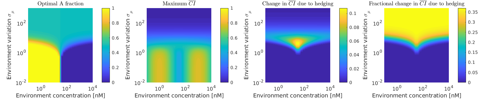
In Fig. 1, we consider two receptor types with dissociation constants and , and numerically determine the fraction of receptors that maximizes . We choose to be log-normal, – a generic option for large variability. When environmental uncertainty is small, we see the behavior predicted above – at small , the cell should express all receptors, while for the cell switches to all-. However, at larger , cells optimize by expressing equal amounts of and receptors (Fig. 1, bottom).
Why is a 50-50 mix optimal even when ? This may seem like a natural response to uncertainty, but it is not obvious why, if the typical concentration, is close to , the cell would not prefer -type receptors. We argue that in the limit of large , where becomes very broad, but is locally peaked, the optimal fraction should not depend on or . The chemotactic index for snapshot sensing is generally peaked when is around or , because the SNR decays when or (Fig. 1, top). As increases and becomes more weakly dependent on , we can approximate the integral defining as
| (2) |
(We’ve chosen as a typical value in the range .) In Eq. 2, the parameters and of the environment distribution only appear in , and the receptor fractions only appear in the term . In this limit, becomes an irrelevant prefactor – the same fraction will optimize independent of and , and so we see a 50-50 mix for a broad range of parameters. We will see later that the 50-50 mix is no longer optimal when cells time average and is no longer locally peaked.
The 50-50 mix between and receptors in Fig. 1 emerges when is so broad it is slowly-varying on the scale of . We caution that at these large levels of environmental variation, the difference between the optimal receptor configuration and simply choosing all- or all- receptors is small (Appendix F) – at sufficiently high uncertainties, no configuration is particularly successful.
Fig. 1 shows when a cell should choose to express a combination of receptor types. Can we also find which receptors a cell would evolve to maximize gradient-sensing ability in a given ? We optimize by varying and receptor fraction for different numbers of receptor types and different widths , holding total receptor number constant. We choose the configuration that maximizes – with an important caveat. By adding more types with arbitrary , we can always at least match the performance of a single type. If many configurations generate roughly the same near-optimal (all within ), we choose from these the configuration with the fewest receptor types . To reduce the number of variables we vary, we use the symmetry of , assuming and are mirror-symmetric around . The resulting optimal are shown in Fig. 2. We see that as the environment uncertainty increases, there is a transition between preferring a single receptor type and multiple receptor types, with the values for the multiple types being spread over the likely range of concentrations observed.
Fig. 1 and Fig. 2 are based on Eq. 1, which gives the fundamental uncertainty for a cell sensing a gradient from a single snapshot of its receptors. If cells integrate measurements over time Ueda and Shibata 2007; Berg and Purcell 1977; Hu et al. 2010; Hu et al. 2011; Endres and Wingreen 2008; ten Wolde et al. 2016, they can improve gradient sensing. Our results in Appendix B give the estimator for the gradient vector given the snapshot data. Defining a time-integrated estimator , as in earlier work Hu et al. 2010; Hu et al. 2011; Camley and Rappel 2017, we find its variance, . To do this, we must consider the kinetics of binding and unbinding at each receptor, which happens with a receptor correlation time of . In the limit of large averaging times , we find (Appendix C):
| (3) |
where reflects the accuracy of measuring by type – maximized at . For a single type, error is reduced by the effective number of measurements , Hu et al. 2010; Hu et al. 2011. Eq. 3 can be cast in a similar form as
where is the weight given to receptor type . This equation shows that the variance – in a naive time average – is reduced by a weighted sum that depends on the receptor correlation times. In the single receptor type case, becomes arbitrarily small as . However, because is proportional to a weighted sum of , when receptor correlation times decrease, error is limited by the slowest correlation time. If one receptor correlation time is significantly faster than another, Eq. 3 predicts reduced error merely by removing the slow receptors (Fig. 3). The naive time average, therefore, does not efficiently use the information available – if it did, the cell would not be able to gain accuracy by throwing away measurements. The core reason for the failure of naive time averaging is that the snapshot estimator weights receptors equally – which is appropriate to the amount of information they provide at that moment. Naively averaging this estimator weighs information from fast receptors (which gain more information as increases) and slow receptors (which gain less information) similarly.
The failure of naive time averaging is reminiscent of a well-known result for concentration sensing: it is not optimal for a single receptor to estimate from a simple time-average of its occupation, . If the whole history of binding and unbinding events is used in a maximum likelihood estimate, the error is reduced by two Endres and Wingreen 2009. We compute the accuracy limit for gradient sensing using the entire receptor trajectory (Appendix D), finding (again in the limit :
| (4) |
or more intuitively,
For a single receptor type, Eq. 4 is a factor of two smaller than the naive time average Eq. 3, precisely as in concentration sensing. However, for multiple types, ERT error can be orders of magnitude better, as the time correlation factors add “in parallel” – error is no longer limited by the slowest type.
We illustrate the differences between these two errors in Fig. 3, computing SNR for two receptor types. Which type provides more information depends on the relative off rates of the two types:
| (5) |
where .
Fig. 3 shows that as is varied, the naive time average SNR is always at least a factor of two lower than ERT. When the receptor off rate is large (), the naive average is worse than if only the receptors were used (the “Naive (fast only)” yellow dotted line). In this limit, most information is from the receptors, and using only receptors reaches half the ERT SNR (Fig. 3).

How does time averaging affect bet-hedging? For a single environmental concentration, all- is optimal when Eq. 5 increases with increasing , i.e. , or . For , it is always best to use the lower- receptor – but trade-offs are more complex when receptors are faster. The balancing point varies from at to at . corresponds to the condition where the on rates of the two types are equal, , as – this would be the case if the on rates were diffusion-limited.
Dependence on receptor off rates is preserved when we study optimal receptor configurations in an uncertain environment . In Fig. 4, we show how the optimal share of receptors depends on . Even with significant uncertainty, when , all- is optimal. However, at higher values of , a transition between all- and all- like Fig. 1 occurs when (white dashed line). By contrast with the snapshot results, in the time average at large uncertainties , the 50-50 mixture is not optimal. Instead, at high uncertainties, for , optimal receptor fractions are similar above and below , and the fraction of receptors exceeds , with decreasing as . Why? When cells time-average, CI is nonzero over a broad range of (see Fig. 4, top), and our argument from the snapshot case fails.
Can we produce a plot such as Fig. 2 showing the optimal receptor configuration if time-averaging is performed? No. When time averaging, error is minimized by making the correlation times as small as possible – taking . We cannot find a consistent set of optimal receptors unless is restricted by some biochemical constraint. This is because, as recognized for concentration sensing Endres and Wingreen 2009, only binding rates are sensitive to – bound times should be minimized.
Discussion.— Our results show that cells can hedge their bets against an uncertain environment by expressing multiple receptor types – but that this behavior is only reasonable if the uncertainty in spans the range of observed (Fig. 2) – i.e. if cells typically explore environments where concentration varies over orders of magnitude. The idea that signal-processing should be adapted to the likely range of concentrations is similar to classical results showing information transmission is maximized by tuning input-output relationships to the input probability distribution Bialek 2012; Barlow 1961; Tkačik et al. 2008; Laughlin 1981. When cells chemotax to hunt bacteria, as Dictyostelium uses folic acid chemotaxis, it is intuitively plausible that observed span orders of magnitude, as bacterial hunting must function over both sparse and concentrated solutions, and over many distances to bacteria. However, at any fixed concentration, expressing multiple receptor types is always suboptimal to choosing the receptor that best fits your current concentration – so hedging is plausible in circumstances when the environment is uncertain over the timescale on which the receptor affinity is fixed. What other timescales could appear in the problem? Dictyostelium receptors are internalized in response to large increases in cAMP concentration Serge et al. 2011; Wang et al. 1988, but this process takes several minutes – much longer than it would typically take Dicty to chemotax to a new mean concentration level. We also show that even if receptor numbers change in different environments, we see very similar results (Appendix E).
Our work has not so far distinguished between truly different receptors and receptors that are phosphorylated or otherwise modified to change their Islam et al. 2018; Xiao et al. 1999, which play a role in adaptation to different signal levels in bacteria Tu and Rappel 2018. If receptor modification is fast compared to the environment’s change in concentration , i.e. can occur before the cell samples a new concentration from , hedging will be less effective. Our work thus suggests interesting future directions for extension, based on recent studies of concentration sensing in time-varying environments Mora and Nemenman 2019. Future work could also consider multiple ligand types, which could also limit accuracy by competing for receptors Mora 2015; Singh and Nemenman 2020. For cells to reach the lower bound of Eq. 4, they must compute estimates with some reaction network, possibly extending recent work showing how to compute the ERT estimate in concentration sensing Singh and Nemenman 2020; Lang et al. 2014. One important difference here is that finding the ERT requires spatially resolved measurements of bound and unbound times separately for each receptor type. Computation of the ERT estimate for concentration requires additional free energy expenditure Lang et al. 2014 – it would be interesting to determine if the extravagant benefits of the ERT approach for gradient sensing with multiple receptor types (Fig. 3) comes with a commensurate cost. Though these are significant complexities, the huge gap between the fundamental bound of Eq. 4 and the naive average of Eq. 3 shows even very rough approximations to the ERT provide significant gains over a naive average.
Acknowledgements.
We thank Wouter-Jan Rappel and Emiliano Perez Ipiña for a close reading of the paper. We thank Allyson Sgro for useful discussions. BAC acknowledges support from the grant PHY-1915491.Notation For Appendix
This appendix includes calculations where we have to distinguish the type and the index of each receptor. The intermediate calculations are more complex than the final results in the main paper, and to help keep the details straight, we will denote receptor types with superscripts and receptor indices with subscripts. A superscript to a power like never denotes exponentiation. To keep consistent with this, we’ve included formulas with where in the main text we’ve written .
Appendix A Numerical details
To evaluate the integral numerically, we found some difficulties that arise because of how broad is. In particular, because the SNR most naturally varies on the log scale (see Fig. 1, top), it is easiest for us to evaluate this expectation in terms of ,
| (6) |
For our log-normal distribution, has the simple Gaussian form
| (7) |
However, we note that even Eq. 6 can be tricky to evaluate when CI is nonzero only for a range of compared with the scale . We evaluate this integral using Matlab’s Gauss-Kronrod quadrature (quadgk), setting waypoints to ensure that all nonzero ranges of both functions should be included.
To find the receptor type fractions that optimize we use Matlab’s fminbnd (golden section search) and fminsearch (Nelder-Mead), depending on the number of variables to be optimized over.
Code to reproduce the results in the paper can be found at: https://github.com/bcamley/hedging_reproduce
Appendix B Snapshot sensing
How precisely can a cell make a measurement of a chemical gradient – using only its current information about which receptors on its surface are occupied? We extend results from Hu et al. 2010; Hu et al. 2011 on this accuracy to include multiple receptor types. We assume that the cell is in a shallow exponential gradient with direction and steepness , where is the diameter of the cell and the concentration at the cell center. The gradient g can also be written as . The concentration at a cell receptor with angular coordinate can then be written as
| (8) |
Let there be receptor types, where there are receptors of type and total receptors. We describe the receptors as being uniformly spread across the cell, with angular positions (Fig. 5). Then each receptor of type can be represented as a Bernoulli trial, i.e. we define a variable that is one if a receptor of type is occupied, and zero otherwise. The probability of is the probability of that receptor being occupied,
| (9) |
where is the concentration at the th receptor of type and is the dissociation constant of receptor type . The dissociation constant is the ratio of unbinding and binding rates of the receptors of type , i.e. Assuming that all the receptors are independent of one another, we have the following likelihood function giving the probability of seeing receptor occupations given gradient
The log-likelihood function is
| (10) | ||||
In the second term in this equation, we then assume that the receptors are numerous enough that we can replace the sum over receptor position by a continuous integral, :
| (11) |
We define and , which measure the spatial asymmetry in the occupancy of receptors of type . and measure the total spatial asymmetry in receptor occupancy of the cell. In a shallow exponential gradient, we can neglect terms and higher for an estimation of the gradient . Then, the log-likelihood function becomes
| (12) |
(We note that past papers with similar derivations Hu et al. 2011; Hopkins and Camley 2019 have not always written the last term in this log-likelihood, which is an irrelevant constant.) Taking the derivative with respect to gives
| (13) |
Because the log function is monotonic, we can set Eq. 13 equal to zero to find and , the parameters which for and which maximize the likelihood function. Carrying out this procedure, we find:
| (14) | ||||
| (15) | ||||
| (16) |
which be solved for to determine estimators as
| (17) |
To determine the asymptotic variance on these estimators, we will need to compute the second derivative of the log-likelihood function. Applying an additional derivative to Eq. 13 gives
| (18) |
From the log-likelihood function, we can also determine the Fisher information matrix, which controls the best possible measurement that the cell can make of the uncertain Hu et al. 2010; Kay 1993. In this case it is diagonal, and its inverse gives the variances of and in the limit of many samples. As a result, we have expressions for the asymptotic variances for and
and so
| (19) |
The important parameter is which is just the sum of the component variances
| (20) |
As the sample size becomes large, the distribution of converges to a normal distribution with means and variance . This also implies that the mean values of and are
| (21) |
Appendix C Naive time averaging
A cell may improve its estimation of the gradient by time averaging. In the previous section, we determined an estimator that is the best estimate of a cell’s gradient, given a snapshot of its receptor information. Naively, a cell could improve its accuracy by making a measurement over a time and determining the average of these estimates
| (22) |
Then the variance of this new estimator will be reduced,
| (23) |
To understand how time averaging improves the cell’s sensing accuracy, we need to compute , the correlation function of . This correlation function is related to the correlation functions in the estimates of each component of the gradient as
| (24) |
And, by Eq. 17, the correlation functions for can be related to the correlation functions for as
| (25) |
The correlation functions for can be written in terms of the single receptor correlation function:
| (26) | ||||
| (27) | ||||
| (28) |
The kinetics of receptor binding and unbinding with multiple receptor types can be quite complicated Wang et al. 2007; Berezhkovskii and Szabo 2013, with ligands potentially diffusing from one receptor to another. However, if the binding and unbinding process is slow with respect to this diffusion – i.e. binding is reaction-limited, as is believed to be the case in eukaryotic chemotaxis Hu et al. 2011; Wang et al. 2007, it is appropriate to think of the ligand-receptor binding having two states – one bound and one with ligand in the bulk. Then, there are two relevant rates, that of ligand binding to a receptor of type exposed to concentration is and the off rate is – which results in an exponential single receptor correlation function
| (29) |
for receptor of type . This limit is also appropriate if all ligand is internalized, as discussed by Endres and Wingreen 2009. The parameter characterizes the fluctuations in the occupancy of the receptor, and is given by
| (30) |
the variance of a Bernoulli trial. is the single receptor correlation time
| (31) |
in the reaction-limited case. (Generalization to other limits is possible but not straightforward Kaizu et al. 2014; Bialek and Setayeshgar 2005; Berezhkovskii and Szabo 2013.) Because different receptors are independent, the mean of their product is just the product of their means
| (32) |
Using Eq. 29 for terms where and and Eq. 32 otherwise, we can expand the correlation function of in Eq. 28 as
| (33) | ||||
| (34) |
The second term in Eq. 34 is , which can be solved as
| (35) |
by Eq. 21. For the first term in Eq. 34, taking the sum to an integral gives
| (36) |
where , i.e., Eq. 31 for a receptor in the ambient concentration . Therefore, for shallow gradients, the correlation function for is
| (37) |
Using the relation in Eq. 25, the correlation function of the estimator can be found from Eq. 37:
| (38) |
Similar expressions for the correlation functions of and can be derived as
| (39) |
and
| (40) |
Thus, the correlation in for shallow gradients is
| (41) |
This now gives us enough information to compute the time-averaged variance,
| (42) |
Then, using the result in Eq. 41, we have
| (43) | ||||
| (44) |
In the limit where for all , Eq. 44 becomes
| (45) |
where the parameter reflects the accuracy of measuring only using receptor , as in the main text.
Appendix D Maximum likelihood using entire receptor binding trajectory (ERT)
Instead of simply performing a naive average, a cell could also improve its sensing of the gradient by determining an estimate of the gradient from the history of its receptors over the measurement time – when they are bound and unbound (Fig. 6). We a time interval for receptor of type as time series , where particles bind at times and unbind at times , where indexes the binding and unbinding events. Following Endres and Wingreen 2009, we compute the probability for a time series of binding and unbinding events. Define a function
which is the probability density for the event that receptor of type experiences an unbinding at time given the previous time series data . Here, the time series has been written for a receptor that is initially unbound, and the indexing of the time series in the following equations will follow that notation. The procedure is the same for a receptor that starts in the bound state. Define the analogous function
for binding events. Then, the probability of observing a time series is given by
| (46) |
where are the numbers of binding events and unbinding events, respectively. If a cell measures for a time interval that is long compared to the relevant time scales (ie, , for all receptor types), then because the number of binding events can differ by at most one from the number of unbinding events. In this limit, the information about the gradient is dominated by the observed time series, and not the initial snapshot state of the receptors.
We assume that we are in the reaction-limited case, where we can treat the rate of binding to a receptor of type exposed to concentration as and the off rate as – neglecting rebinding. (Neglecting rebinding, as discussed in more detail by Endres and Wingreen 2009, is also the appropriate limit to find the fundamental bound to accuracy, as cells may prohibit rebinding by degrading or internalizing ligand.) The functions and , with this simple Markovian kinetics, do not depend on the whole time series, they only depend on the time of previous unbinding/binding event:
| (47) | ||||
| (48) |
These are probability density functions for exponential distributions with rates and for unbinding and binding, respectively. From these equations, we can determine the likelihood function for the gradient parameters and given the observed time series at receptors of types . Because each receptor is independent, the likelihood function is the product of the probability function in Eq. 46:
| (49) |
Then, define the total time bound and the total time unbound for receptor of type (the indexing in these definitions assume the receptor starts unbound, but analogous definitions can be written for a receptor that is bound at , and in the limit of long times treated here, this assumption does not matter.)
| (50) | ||||
| (51) |
With these definitions, the likelihood function in Eq. 49 becomes
The log-likelihood function is then
| (52) |
Substituting the expression in Eq. 52 gives
| (53) |
For shallow gradients, we can approximate the log-likelihood function by expanding to second order in the magnitude of the gradient. This results in
| (54) |
Differentiating Eq. 54 with respect to and , we get
| (55) |
| (56) |
Because and here do not depend on and , Eq. 56 can be equated to zero and solved to find the maximum likelihood estimator in terms of sums over functions of and . However, we have not found the precise form very useful. From the derivatives of the log-likelihood function, we can compute the Fisher Information Matrix:
| (57) |
Differentiating Eq. 55 and Eq. 56 with respect to combinations of and gives the following matrix
| (58) |
The expectation value can be found in terms of the measurement time and the probability that a receptor is occupied (Eq. 9)
| (59) |
By substituting Eq. 59 into Eq. 58 and taking the inner sums to an integral, we have the following expressions for each matrix element:
| (60) |
| (61) |
| (62) |
Therefore, the Fisher information matrix is diagonal, and in shallow gradients it is
| (63) |
We note that Eq. 63 has only been calculated in the large- limit; in the limit of , we would expect the Fisher information to limit to the estimate from a single snapshot.
For cells with a single receptor type, Eq. 63 implies that the asymptotic variances on and are 1/2 of their value determined from time averaging—the same factor as in concentration sensing Endres and Wingreen 2009. However, in the multiple receptor type case, there is a more significant difference. The variance in determined from Eq. 63 is the sum of the inverses of the diagonal elements
| (64) |
As discussed in the main text, this shows that a slow receptor correlation does not act as a limiting factor when the entire receptor trajectory is considered.
Appendix E Hedging allowing the number of receptors to change
Within the main text, we have followed earlier work in keeping the number of receptors on the cell fixed Hu et al. 2010; Hu et al. 2011; Segota et al. 2013; Lakhani and Elston 2017; Fuller et al. 2010; Ueda and Shibata 2007; Andrews and Iglesias 2007. However, it is possible that when cells explore more complex environments, they should express different numbers of receptors depending on the typical concentration and the level of uncertainty . We address this possibility in Fig. 7.

Within the framework we have applied in this paper, accuracy always increases with increasing – there are more measurements of the gradient, leading to increased accuracy (see Eq. 1,3,4 in the main text). If we allow the number of receptors to freely vary, and choose the number of receptors and receptor fractions , we would find that the receptor number would increase without bound. This is obviously unphysical. Cells are under many restraints in controlling how many receptors they have, both in terms of the energetic cost of synthesizing them, and in the opportunity cost in taking up space on the cell surface.
In modeling cells with varying receptor number, we chose to find the receptor configuration that maximized , where is the number of receptors expressed beyond the typical value , and . This choice ensured that cells could easily express more than the basal level of receptors, but that expressing multiple orders of magnitude more receptors would be implausible – consistent with the observed variation in receptor number on the membrane. We found that, though the optimal receptor numbers varied depending on the environment (Fig. 7), the optimal receptor fractions closely agreed with those found assuming a constant number of receptors (Fig. 1).
Other choices for the penalty (e.g. optimizing ) gave different optimal receptor numbers but preserved the optimal receptor fractions and the transition between all-A, all-B, and the 50-50 mix. This suggests that the receptor fractions and the transition are highly robust to allowing the number of receptors to change. This may reflect that the optimal fractions are only very weakly dependent on the total number of receptors.
Experimental measurements on Dictyostelium do see that receptors are internalized in response to saturating levels of chemoattractant; however, this happens on a long time scale ( minutes) and results in a change of about 50% of the receptors being internalized Serge et al. 2011; Wang et al. 1988. For Dictyostelium cells, which travel about a body length in a minute, we would expect that crawling cells would likely explore another concentration level before the receptor numbers adapt. Adaptation in eukaryotic chemotaxis is generally thought to occur on a post-receptor level Tu and Rappel 2018; Takeda et al. 2012.
Appendix F Extended data on hedging
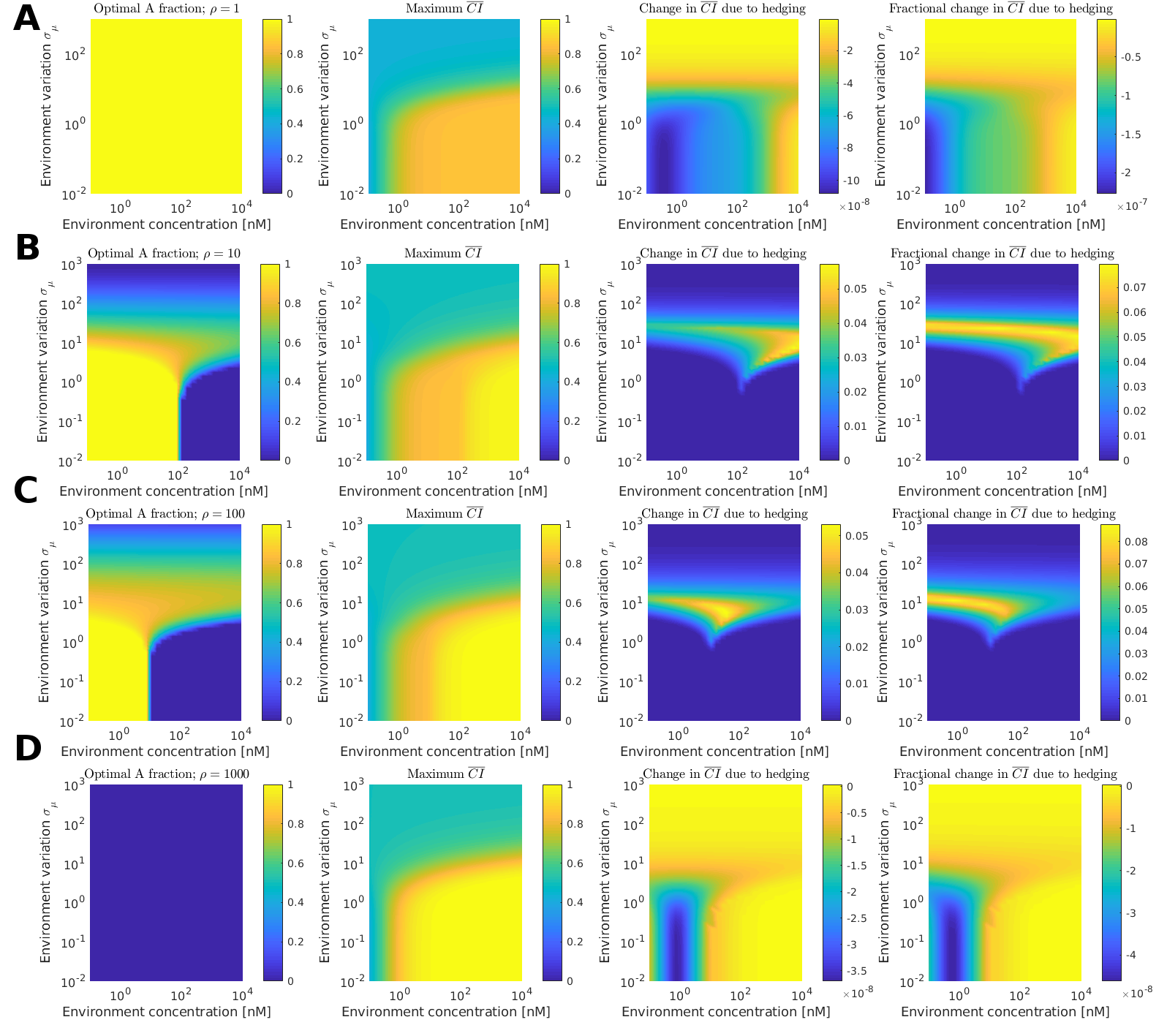
Within the main paper, we have presented the optimal configuration of receptors as a function of the environment. However, at large environmental uncertainties, the benefit from hedging bets may not be as large. We show extended data corresponding to Fig. 1 and Fig. 4 in the main paper in Fig. 8 and Fig. 9.
References
- Levine and Rappel (2013) Herbert Levine and Wouter-Jan Rappel, “The physics of eukaryotic chemotaxis,” Physics Today 66 (2013).
- Fuller et al. (2010) Danny Fuller, Wen Chen, Micha Adler, Alex Groisman, Herbert Levine, Wouter-Jan Rappel, and William F Loomis, “External and internal constraints on eukaryotic chemotaxis,” Proceedings of the National Academy of Sciences 107, 9656 (2010).
- Ueda and Shibata (2007) Masahiro Ueda and Tatsuo Shibata, “Stochastic signal processing and transduction in chemotactic response of eukaryotic cells,” Biophysical Journal 93, 11 (2007).
- Segota et al. (2013) Igor Segota, Surin Mong, Eitan Neidich, Archana Rachakonda, Catherine J Lussenhop, and Carl Franck, “High fidelity information processing in folic acid chemotaxis of Dictyostelium amoebae,” Journal of The Royal Society Interface 10, 20130606 (2013).
- Hu et al. (2010) Bo Hu, Wen Chen, Wouter-Jan Rappel, and Herbert Levine, “Physical limits on cellular sensing of spatial gradients,” Physical Review Letters 105, 048104 (2010).
- Endres and Wingreen (2008) Robert G Endres and Ned S Wingreen, “Accuracy of direct gradient sensing by single cells,” Proceedings of the National Academy of Sciences 105, 15749 (2008).
- Shi et al. (2013) Changji Shi, Chuan-Hsiang Huang, Peter N Devreotes, and Pablo A Iglesias, “Interaction of motility, directional sensing, and polarity modules recreates the behaviors of chemotaxing cells,” PLoS computational biology 9, e1003122 (2013).
- Hecht et al. (2011) Inbal Hecht, Monica L Skoge, Pascale G Charest, Eshel Ben-Jacob, Richard A Firtel, William F Loomis, Herbert Levine, and Wouter-Jan Rappel, “Activated membrane patches guide chemotactic cell motility,” PLoS Computational Biology 7 (2011).
- Camley (2018) Brian A Camley, “Collective gradient sensing and chemotaxis: modeling and recent developments,” Journal of Physics: Condensed Matter 30, 223001 (2018).
- Camley and Rappel (2017) Brian A Camley and Wouter-Jan Rappel, “Cell-to-cell variation sets a tissue-rheology–dependent bound on collective gradient sensing,” Proceedings of the National Academy of Sciences 114, E10074–E10082 (2017).
- Mugler et al. (2016) Andrew Mugler, Andre Levchenko, and Ilya Nemenman, “Limits to the precision of gradient sensing with spatial communication and temporal integration,” Proceedings of the National Academy of Sciences , 201509597 (2016).
- Hopkins and Camley (2019) Austin Hopkins and Brian A Camley, “Leader cells in collective chemotaxis: Optimality and trade-offs,” Physical Review E 100, 032417 (2019).
- Sharma and Roberts (2016) Rati Sharma and Elijah Roberts, “Gradient sensing by a bistable regulatory motif enhances signal amplification but decreases accuracy in individual cells,” Physical Biology 13, 036003 (2016).
- Lakhani and Elston (2017) Vinal Lakhani and Timothy C Elston, “Testing the limits of gradient sensing,” PLoS Computational Biology 13, e1005386 (2017).
- de Wit and van Haastert (1985) RenéJ W de Wit and Peter JM van Haastert, “Binding of folates to Dictyostelium discoideum cells. demonstration of five classes of binding sites and their interconversion,” Biochimica et Biophysica Acta (BBA)-Biomembranes 814, 199–213 (1985).
- Johnson et al. (1992) Ronald L Johnson, PJ Van Haastert, Alan R Kimmel, Charles L Saxe, Bernd Jastorff, and Peter N Devreotes, “The cyclic nucleotide specificity of three cAMP receptors in Dictyostelium.” Journal of Biological Chemistry 267, 4600–4607 (1992).
- Hereld and Devreotes (1993) Dale Hereld and Peter N Devreotes, “The cAMP receptor family of dictyostelium,” International review of cytology , 35–35 (1993).
- Kim et al. (1998) JY Kim, JA Borleis, and Peter N Devreotes, “Switching of chemoattractant receptors programs development and morphogenesis in Dictyostelium: Receptor subtypes activate common responses at different agonist concentrations,” Developmental Biology 197, 117–128 (1998).
- Dormann et al. (2001) Dirk Dormann, Ji-Yun Kim, Peter N Devreotes, and Cornelis J Weijer, “cAMP receptor affinity controls wave dynamics, geometry and morphogenesis in Dictyostelium,” Journal of Cell Science 114, 2513–2523 (2001).
- Hu et al. (2011) Bo Hu, Wen Chen, Wouter-Jan Rappel, and Herbert Levine, “How geometry and internal bias affect the accuracy of eukaryotic gradient sensing,” Physical Review E 83, 021917 (2011).
- Camley et al. (2016) Brian A Camley, Juliane Zimmermann, Herbert Levine, and Wouter-Jan Rappel, “Emergent collective chemotaxis without single-cell gradient sensing,” Physical Review Letters 116, 098101 (2016).
- Berg and Purcell (1977) Howard C Berg and Edward M Purcell, “Physics of chemoreception.” Biophysical Journal 20, 193 (1977).
- ten Wolde et al. (2016) Pieter Rein ten Wolde, Nils B Becker, Thomas E Ouldridge, and Andrew Mugler, “Fundamental limits to cellular sensing,” Journal of Statistical Physics 162, 1395–1424 (2016).
- Endres and Wingreen (2009) Robert G Endres and Ned S Wingreen, “Maximum likelihood and the single receptor,” Physical Review Letters 103, 158101 (2009).
- Bialek (2012) William Bialek, Biophysics: searching for principles (Princeton University Press, 2012).
- Barlow (1961) Horace B Barlow, “Possible principles underlying the transformation of sensory messages,” Sensory communication 1, 217–234 (1961).
- Tkačik et al. (2008) Gašper Tkačik, Curtis G Callan, and William Bialek, “Information flow and optimization in transcriptional regulation,” Proceedings of the National Academy of Sciences 105, 12265–12270 (2008).
- Laughlin (1981) Simon Laughlin, “A simple coding procedure enhances a neuron’s information capacity,” Zeitschrift für Naturforschung c 36, 910–912 (1981).
- Serge et al. (2011) Arnauld Serge, Sandra de Keijzer, Freek Van Hemert, Mark R Hickman, Dale Hereld, Herman P Spaink, Thomas Schmidt, and B Ewa Snaar-Jagalska, “Quantification of gpcr internalization by single-molecule microscopy in living cells,” Integrative Biology 3, 675–683 (2011).
- Wang et al. (1988) Mei Wang, Peter JM Van Haastert, Peter N Devreotes, and Pauline Schaap, “Localization of chemoattractant receptors on Dictyostelium discoideum cells during aggregation and down-regulation,” Developmental Biology 128, 72–77 (1988).
- Islam et al. (2018) AFM Tariqul Islam, Haicen Yue, Margarethakay Scavello, Pearce Haldeman, Wouter-Jan Rappel, and Pascale G Charest, “The cAMP-induced G protein subunits dissociation monitored in live Dictyostelium cells by BRET reveals two activation rates, a positive effect of caffeine and potential role of microtubules,” Cellular signalling 48, 25–37 (2018).
- Xiao et al. (1999) Zhan Xiao, Yihong Yao, Yu Long, and Peter Devreotes, “Desensitization of G-protein-coupled receptors,” Journal of Biological Chemistry 274, 1440–1448 (1999).
- Tu and Rappel (2018) Yuhai Tu and Wouter-Jan Rappel, “Adaptation in living systems,” Annual Review of Condensed Matter Physics 9, 183–205 (2018).
- Mora and Nemenman (2019) Thierry Mora and Ilya Nemenman, “Physical limit to concentration sensing in a changing environment,” Physical Review Letters 123, 198101 (2019).
- Mora (2015) Thierry Mora, “Physical limit to concentration sensing amid spurious ligands,” Physical Review Letters 115, 038102 (2015).
- Singh and Nemenman (2020) Vijay Singh and Ilya Nemenman, “Universal properties of concentration sensing in large ligand-receptor networks,” Physical Review Letters 124, 028101 (2020).
- Lang et al. (2014) Alex H Lang, Charles K Fisher, Thierry Mora, and Pankaj Mehta, “Thermodynamics of statistical inference by cells,” Physical Review Letters 113, 148103 (2014).
- Kay (1993) Steven M Kay, “Fundamentals of statistical signal processing,” PTR Prentice-Hall, Englewood Cliffs, NJ (1993).
- Wang et al. (2007) Kai Wang, Wouter-Jan Rappel, Rex Kerr, and Herbert Levine, “Quantifying noise levels of intercellular signals,” Physical Review E 75, 061905 (2007).
- Berezhkovskii and Szabo (2013) Alexander M Berezhkovskii and Attila Szabo, “Effect of ligand diffusion on occupancy fluctuations of cell-surface receptors,” The Journal of Chemical Physics 139, 121910 (2013).
- Kaizu et al. (2014) Kazunari Kaizu, Wiet de Ronde, Joris Paijmans, Koichi Takahashi, Filipe Tostevin, and Pieter Rein ten Wolde, “The Berg-Purcell limit revisited,” Biophysical Journal 106, 976 (2014).
- Bialek and Setayeshgar (2005) William Bialek and Sima Setayeshgar, “Physical limits to biochemical signaling,” Proceedings of the National Academy of Sciences of the United States of America 102, 10040 (2005).
- Andrews and Iglesias (2007) Burton W Andrews and Pablo A Iglesias, “An information-theoretic characterization of the optimal gradient sensing response of cells,” PLoS Comput Biol 3, e153 (2007).
- Takeda et al. (2012) Kosuke Takeda, Danying Shao, Micha Adler, Pascale G Charest, William F Loomis, Herbert Levine, Alex Groisman, Wouter-Jan Rappel, and Richard A Firtel, “Incoherent feedforward control governs adaptation of activated Ras in a eukaryotic chemotaxis pathway,” Science Signaling 5, ra2 (2012).