跳到论文正文
W Papers独立论文阅读器 arXiv:2002.10415 论文正文 计算阅读时间 · 0%
引用这篇论文根据当前论文元数据生成,正式投稿前建议核对。


License: arXiv.org perpetual non-exclusive license
arXiv:2002.10415v3 [econ.EM] 10 Mar 2022

Extending Economic Models with Testable Assumptions: Theory and Applications

Moyu Liao Thanks: I would like to thank Marc Henry for his invaluable advice and encouragement. I also thank Andres Aradillas-Lopez and Keisuke Hirano, Michael Gechter, Patrik Guggenberger, Sun Jae Jun, and Joris Pinkse for their useful comments. Affiliation: Nanjing University
Abstract

This paper studies the identification and hypothesis testing in complete and incomplete economic models with testable assumptions. A testable assumption (AA) gives interpretable empirical content to the economic model but it also carry the possibility that some distributions of observed outcomes may reject these assumptions. A way to avoid the data rejection problem is to find a relaxed assumptions (A~\tilde{A}) that cannot be rejected by any distribution of observed outcomes. We also want the identified set for the parameter of interest under A~\tilde{A} is not changed when the original assumption AA is not rejected by the observed data distribution. I characterize the properties of such a relaxed assumption A~\tilde{A} using a generalized notion of refutability and confirmability. I also propose a general method to construct such A~\tilde{A}. I apply my methodology to the instrument monotonicity assumption in Local Average Treatment Effect (LATE) estimation and to the sector selection assumption in a binary outcome Roy model of employment sector choice. In the LATE application, I use my general method to construct a relaxed assumption A~\tilde{A} that can never be rejected, and the identified set for LATE is unchanged when AA holds. LATE is point identified under my extension A~\tilde{A} in the application. In the binary outcome Roy model, I use my method to relax Roy’s sector selection assumption and characterize the identified set for the binary potential outcomes as a polyhedron.

Keywords— Incomplete Models; Refutability; LATE; Roy Model

JEL— C12, C13, C18, C51, C52

1 Introduction

Empirical researchers often make convenient model assumptions in structural estimation. These assumptions usually come from economic theories or intuitions. For example, the ‘No Defiers’ assumption in Imbens and Angrist 1994 assumes that the instrument has a monotone effect on the decision to take treatment; the ‘Pure Strategy Nash Equilibrium’ assumption in Bresnahan and Reiss 1991 assumes only pure strategy Nash Equilibrium is played in a 2×22\times 2 entry game; the ‘Perfect Self Selection’ assumption in Roy 1951 assumes employees perfectly observe their future earnings and choose a job sector to maximize discounted lifetime earnings. Such assumptions simplify the identification and estimation problems, and make the results easier to interpret. To study structural models and economic assumptions, I generalize the language of econometric structures (Koopmans and Reiersol 1950) to incomplete structures. A (generalized) econometric structure includes a distribution of some exogenously given latent and observed variables, and a correspondence from the distribution of these exogenous variables to a set of distributions of observed variables. Assumptions are restrictions on the economic structures to reflect empirical researchers’ understanding of the economic environment.

Unfortunately, assumptions in the three examples above, when combined with some other reasonable assumptions, can be rejected by some distributions of observables (Kitagawa 2015; Mourifié and Wan 2017; Mourifie et al. 2018). When the imposed assumption is refuted by data, the econometrician have an empty identified set for the parameter of interest. As a result, the econometrician cannot give a useful interpretation of the economic environment. A refutable assumption AA also imposes challenges to the interpretation of hypothesis testing of parameter values. For example, when we reject the null hypothesis that the parameter equals zero under AA, it can either be the case that the true parameter equals another value, or the case that AA is rejected data. These two cases cannot be distinguished but they have quite different interpretations.

A way to prevent the data rejection problem is to find a relaxed assumption A~\tilde{A} so that no distributions of observables can reject A~\tilde{A}. We call this the non-refutability criterion. By imposing a non-refutable A~\tilde{A} before confronting the data, practitioners avoid the ex-post possibility of finding data evidence against their assumption. Therefore, non-refutability is the first criterion for the relaxed assumption A~\tilde{A} to satisfy. On the other hand, we also do not want to deviate from the old assumption AA, since it still reflects the economic theory behind it. Specifically, given a parameter of interest θ\theta as a function of structures, we want the (sharp) identified set under the relaxed assumption A~\tilde{A} to be equal to the (sharp) identified set under AA, when AA is not rejected by the observed distribution. In other words, we want to preserve the identified set.

This paper aims to do three things: First, I formalize and extend the definition of refutability and confirmability of assumptions in Breusch 1986 using the language of generalized economic structures. These definitions are useful to characterize properties of a relaxed assumption A~\tilde{A}. I characterize conditions that a relaxed assumption A~\tilde{A} needs to satisfy so that: (a).No distribution of observables can be rejected under A~\tilde{A}; (b).The identified sets for the parameter of interest under AA and A~\tilde{A} are the same whenever AA is not rejected by the observed data distribution. I show that when structures are complete, a relaxed assumption A~\tilde{A} that satisfies the two properties above always exists. I also characterize a sufficient condition for the existence of A~\tilde{A} in case of incomplete structures. The possible failure to find A~\penalty\ \tilde{A} in incomplete structures encourages researchers to complete the structures, and then find a nice relaxed assumption in the completed structure universe. When the structures are complete, I also provide a general method to construct A~\tilde{A} from AA.

Second, I discuss the problem of testing hypothesis on structural parameters’ values. I show that any statistical test cannot achieve pointwise size control and test consistency simultaneously when the null hypothesis of structural parameters does not induce a partition of the space of distribution of observables. This is an ill-behaved null hypothesis, and policy decisions based on the result of hypothesis testing can be problematic. Conversely, with a well-behaved null hypothesis, which induces a partition of the space of distribution of observables, I show the existence of statistical tests that achieve pointwise size control and test consistency simultaneously under mild conditions. I also show that when the parameter of interest θ\theta is point identified, a null hypothesis on the value of θ\theta is always well-behaved. When structures are complete, I also provide a way to minimally extend (resp. shrink) the null hypothesis set such that the extend (resp. shrink) hypothesis is well-behaved.

Third, I look at 2 applications with complete and incomplete structures respectively. In the complete structure framework, I look at the identification of the local average treatment effects (LATE). Kitagawa 2015 provides the sharp testable implication of the Imbens and Angrist Monotonicity assumption (IA-M). Therefore, practitioners should anticipate the IA-M to be rejected by some distributions of observables. I provide several relaxations of the IA-M that cannot be rejected by any distribution of observables. The identified sets for LATE under these relaxed assumptions equal the identified set for LATE under the IA-M whenever the IA-M is not rejected by the distributions of observables. One relaxed assumption allows for defiers, and relaxes the independent instrument assumption. The logic of the relaxed assumption is to allow a minimal mass of defiers. It can be shown that the relaxed assumption not only preserves the identified set for LATE, but also preserves the identified set for other parameters of interests such as ATE or ATT. LATE is point identified under this relaxed assumption. I provide an estimator of the LATE which has a normal limit distribution. To emphasis the fact that a non-refutable relaxation is not unique, I propose two other relaxations, each one of which may be preferable in some contexts. I apply the method to Card 1993, and I show the local average treatment effect of education on earnings. Compared to naively using identification result under the IA-M assumption, my method delivers more reasonable sign and scale for the LATE estimates.

For incomplete structures, I look at a binary outcome job sector selection model with a monotone instrument. In the sector choice model, the Roy assumption does not specify the sector choice rule in case of ties, which may lead to multiple predicted distributions of observables. After completing the structures, I then use a ‘minimal efficiency loss’ criterion to characterize the relaxed assumption. The identified set of job sector potential outcome distribution can be characterized as a polyhedron.

Related Literature

Masten and Poirier 2018 propose an ex-post way to salvage a refutable assumption AA. Their ex-post method characterizes a relaxation of AA after the distribution of observables is realized. This paper also relates to the literature that relaxes assumption make model robust to misspecification. In the macroeconomic literature, researchers use robust control to avoid the misspecification issue in their baseline model (see Hansen et al. 2006 and Hansen and Sargent 2007). The Robust control approach aims to accommodate local perturbations to the baseline model rather than to solve the refutability of the baseline model.11 1 The perturbation is usually measured by relative entropy the in macroeconomic literature. It may be true that the baseline model is not refutable by any data distribution. See Bonhomme and Weidner 2018 and Christensen and Connault 2019 for more discussion.

This paper also contributes to the literature that relaxes the IA-M assumption. De Chaisemartin 2017 discusses the economic meaning of the conventional LATE quantity L​A​T​EW​a​l​d≡(E⁡[Yi|Zi=1]−E⁡[Yi|Zi=0])/(E⁡[Di|Zi=1]−E⁡[Di|Zi=0])LATE^{Wald}\equiv({E[Y_{i}|Z_{i}=1]-E[Y_{i}|Z_{i}=0]})/({E[D_{i}|Z_{i}=1]-E[D_{i}|Z_{i}=0]}) when there are defiers. He shows that the L​A​T​EW​a​l​dLATE^{Wald} identifies the net average treatment effect of a subgroup of compliers after deducting the average treatment effect of defiers.

The rest of the paper is organized as follows. Section 2 describes a theory of characterizing a refutable assumption A~\tilde{A}, finding a relaxed assumption A~\tilde{A} and hypothesis testing. Core definitions in Section 2 are followed by shadowed links where their corresponding illustrations can be found. Section 3 applies complete structure theory to the model in Imbens and Angrist 1994. Section 4 applies the theory to a binary outcome Roy model. Main proofs are collected in Appendices. Additional proofs and results are collected in the Online Appendices.

Notations

Throughout this paper, I use XX to denote the vector of observed variables, and I use FF to denote the distribution of XX. I use ϵ\epsilon to denote the vector of latent variables and some observed variables, and I use GG to denote the distribution of ϵ\epsilon. I use ss to denote an economic structure. I use AA to denote a refutable assumption and use A~\tilde{A} to denote a relaxed assumption. I use 𝔽n\mathbb{F}_{n} to denote the empirical distribution of FF.

2 A Theory of Identification and Hypothesis Testing

In this section, I develop a theory for identification and refutable assumptions. I will then discuss the problem of hypothesis testing. I start with a definition of the observation space.

Definition 2.1.

The observation space ℱ\mathcal{F} is the collection of all possible distribution of F⁡(X)F(X). See 3.2 for an illustration.

The distribution of observables F⁡(X)F(X) is generated by some distribution of underlying random vectors ϵ\epsilon through some mapping MM. A pair of a distribution of ϵ\epsilon and a mapping MM is called an econometric structure. The following definition of econometric structure is a reformulation of the economic structure defined in Koopmans and Reiersol 1950 and Jovanovic 1989. Since in most econometric problems, we focus on the distribution of outcomes FF instead of how each XX is related to ϵ\epsilon, I directly define the mapping MM as a correspondence from the space of underlying variable distributions to ℱ\mathcal{F}.

Definition 2.2.

An econometric structure (Model) s=(Gs,Ms)s=(G^{s},M^{s}) consists of a distribution GsG^{s}, and an outcome mapping MsM^{s}. Let 𝒢\mathcal{G} denote the space of all possible regular distributions of Gs​(ϵ)G^{s}(\epsilon). The outcome mapping MsM^{s} is a correspondence Ms:𝒢⇉ℱM^{s}:\mathcal{G}\rightrightarrows\mathcal{F}. See (3.3),(3.4), (4.3) for illustrations.

Definition 2.3.

A structure universe 𝒮\mathcal{S} is a collection of structures such that ∪s∈𝒮Ms(Gs)=ℱ\cup_{s\in\mathcal{S}}M^{s}(G^{s})=\mathcal{F}, and an assumption AA is a subset of 𝒮\mathcal{S}. See (3.5),(3.7),(4.4), (4.6) for illustrations.

The mapping MsM^{s} of structure ss relates the distribution ϵ\epsilon to the distributions of XX. Since the distributions of XX are generated by the distributions of ϵ\epsilon, we call ϵ\epsilon the primitive variables. Definition 2.3 allows overlap between XX and ϵ\epsilon. A collection of structures is called a structure universe. We want to learn the distribution of ϵ\epsilon and the mapping MM from the distribution of observables FF.

Here I explicitly distinguish the structure universe 𝒮\mathcal{S} and the assumption AA, though both are just a collection of structures. The structure universe 𝒮\mathcal{S} is the paradigm that can span different empirical contexts. On the other hand, an assumption AA places constraints that are suitable for a particular empirical context, or convenient for empirical analysis.

The condition ∪s∈𝒮Ms(Gs)=ℱ\cup_{s\in\mathcal{S}}M^{s}(G^{s})=\mathcal{F} requires that all possible distributions of observables can be generated by some structure in the universe. Moreover, no distribution outside ℱ\mathcal{F} can be generated by 𝒮\mathcal{S}.

Definition 2.4.

A structure s:=(Ms,Gs)s:=(M^{s},G^{s}) is called complete if Ms​(Gs)M^{s}(G^{s}) is a singleton. Otherwise it is called incomplete. A universe 𝒮\mathcal{S} is called complete if every structure ss in 𝒮\mathcal{S} is complete, otherwise it is incomplete.

The definition of completeness is slightly different from the definition of completeness in Tamer 2003. Tamer 2003 defines a model to be complete if the mapping from ϵ\epsilon to XX is a singleton and non-empty, and incomplete if the mapping has multiple outputs, and incoherent if the mapping generates no output. Here, my definition of economic structure does not specify the mapping from each ϵ\epsilon to XX. Instead, I consider the mapping from the distribution of ϵ\epsilon to the distribution of XX. If the probability of multiple outcome is non-zero, an incomplete model in Tamer 2003 implies an incomplete structure in my definition.

My definition of structure, however, does not have a corresponding terminology for incoherent model. This is because I require ∪s∈𝒮Ms(Gs)=ℱ\cup_{s\in\mathcal{S}}M^{s}(G^{s})=\mathcal{F} to hold. Chesher and Rosen 2012 propose four ways to deal with model incoherence and derive the distribution of observables under the model. My definition of MsM^{s} as the mapping between distributions can be viewed as the consequences of Chesher and Rosen 2012.

Definition 2.5.

(Breusch) An assumption AA is called refutable if there exists an F∈ℱF\in\mathcal{F} such that F∉∪s∈AMs(Gs)F\notin\cup_{s\in A}M^{s}(G^{s}). An assumption AA is called confirmable if there exists an F∈ℱF\in\mathcal{F} such that F∉∪s∈AcMs(Gs)F\notin\cup_{s\in A^{c}}M^{s}(G^{s}).

The notions of refutability and confirmability of a complete structure are given in Breusch 1986. If an assumption is refutable, then there exists some FF that can reject AA. The notions of refutability and confirmability are stated in terms of the observation space ℱ\mathcal{F}. Equivalently, we can characterize refutability and confirmability in terms of the structure universe 𝒮\mathcal{S}. To do this, I first define the non-refutability and confirmation sets associated with AA.

Definition 2.6.

(non-refutability set)
The strong non-refutability set associated with AA under 𝒮\mathcal{S} is defined as

ℋ𝒮s​n​f(A)={s∈𝒮:Ms(Gs)⊆∪s∗∈AMs∗(Gs∗)}.\mathcal{H}^{snf}_{\mathcal{S}}(A)=\left\{s\in\mathcal{S}:M^{s}(G^{s})\subseteq\cup_{s^{*}\in A}M^{s^{*}}(G^{s^{*}})\right\}.

The weak non-refutability set associated with AA under 𝒮\mathcal{S} is defined as

ℋ𝒮w​n​f(A)={s∈𝒮:Ms(Gs)∩(∪s∗∈AMs∗(Gs∗))≠∅}.\mathcal{H}^{wnf}_{\mathcal{S}}(A)=\left\{s\in\mathcal{S}:M^{s}(G^{s})\cap\left(\cup_{s^{*}\in A}M^{s^{*}}(G^{s^{*}})\right)\neq\varnothing\right\}.

See Lemma 3.1, (3.8) and Proposition 4.1 for illustrations.

To accommodate the incomplete structures, we define two types of non-refutability sets. We call ℋ𝒮s​n​f​(A)\mathcal{H}_{\mathcal{S}}^{snf}(A) the strong non-refutability set associated with AA, because if the true structure ss is in ℋ𝒮s​n​f​(A)\mathcal{H}_{\mathcal{S}}^{snf}(A), then for any distributions of observables in Ms​(Gs)M^{s}(G^{s}), we cannot refute AA. In contrast, we call ℋ𝒮w​n​f​(A)\mathcal{H}_{\mathcal{S}}^{wnf}(A) the strong non-refutability set associated with AA, because if the true structure ss is in ℋ𝒮w​n​f​(A)\mathcal{H}_{\mathcal{S}}^{wnf}(A), then for some distributions of observables in Ms​(Gs)M^{s}(G^{s}), we cannot refute AA.

Definition 2.7.

(Confirmation set)
The strong confirmation set associated with AA under S{S} is defined as

ℋSs​c​o​n(A)={s∈S:Ms(Gs)⊆∩s∗∈Ac(Ms∗(Gs∗)c)}.\mathcal{H}_{S}^{scon}(A)=\left\{s\in{S}:M^{s}(G^{s})\subseteq\cap_{s^{*}\in A^{c}}\left(M^{s^{*}}(G^{s^{*}})^{c}\right)\right\}.

The weak confirmation set associated with AA under S{S} is defined as

ℋSw​c​o​n(A)={s∈S:Ms(Gs)∩[∩s∗∈Ac(Ms∗(Gs∗)c)]≠∅}.\mathcal{H}_{S}^{wcon}(A)=\left\{s\in{S}:M^{s}(G^{s})\cap\left[\cap_{s^{*}\in A^{c}}\left(M^{s^{*}}(G^{s^{*}})^{c}\right)\right]\neq\varnothing\right\}.

See Proposition 4.1 for an illustration.

The strong confirmation set is the collection of structures that cannot be observationally equivalent to any structures outside AA for any observed distribution FF. Weak confirmation set is the collection of structures that cannot be observationally equivalent to any structures outside AA for some observed distribution FF. I call ℋ𝒮s​c​o​n​(A)\mathcal{H}^{scon}_{\mathcal{S}}(A) (resp. ℋ𝒮w​c​o​n​(A)\mathcal{H}^{wcon}_{\mathcal{S}}(A)) the strong (resp. weak) confirmation set associated with AA, because if the true structure ss is in ℋ𝒮s​c​o​n​(A)\mathcal{H}^{scon}_{\mathcal{S}}(A) (resp. ℋ𝒮w​c​o​n​(A)\mathcal{H}^{wcon}_{\mathcal{S}}(A)), then for all (resp. some) distribution of observables in Ms​(Gs)M^{s}(G^{s}), we can confirm that the true structure must lies in AA. In particular,

ℋ𝒮s​c​o​n​(A)⊆ℋ𝒮w​c​o​n​(A)⊆A⊆ℋ𝒮s​n​f​(A)⊆ℋ𝒮w​n​f​(A).\mathcal{H}_{\mathcal{S}}^{scon}(A)\subseteq\mathcal{H}_{\mathcal{S}}^{wcon}(A)\subseteq A\subseteq\mathcal{H}_{\mathcal{S}}^{snf}(A)\subseteq\mathcal{H}_{\mathcal{S}}^{wnf}(A).

When the structure universe 𝒮\mathcal{S} is complete, Ms​(Gs)M^{s}(G^{s}) is always a singleton, and ℋ𝒮s​c​o​n​(A)=ℋ𝒮w​c​o​n​(A)\mathcal{H}_{\mathcal{S}}^{scon}(A)=\mathcal{H}_{\mathcal{S}}^{wcon}(A), ℋ𝒮s​n​f​(A)=ℋ𝒮w​n​f​(A)\mathcal{H}_{\mathcal{S}}^{snf}(A)=\mathcal{H}_{\mathcal{S}}^{wnf}(A). The following proposition helps to interpret the confirmation sets associated with AA as the non-refutability sets associated with AcA^{c}. It also shows that the strong non-refutability set and weak confirmation set as operation are idempotent.

Proposition 2.1.

The following holds: 1. [ℋ𝒮s​n​f​(A)]c=ℋ𝒮w​c​o​n​(Ac)\left[\mathcal{H}_{\mathcal{S}}^{snf}(A)\right]^{c}=\mathcal{H}_{\mathcal{S}}^{wcon}(A^{c}); 2. [ℋ𝒮w​n​f​(A)]c=ℋ𝒮s​c​o​n​(Ac)\left[\mathcal{H}_{\mathcal{S}}^{wnf}(A)\right]^{c}=\mathcal{H}_{\mathcal{S}}^{scon}(A^{c}); 3. ℋ𝒮w​c​o​n​(ℋ𝒮w​c​o​n​(A))=ℋ𝒮w​c​o​n​(A)\mathcal{H}_{\mathcal{S}}^{wcon}(\mathcal{H}_{\mathcal{S}}^{wcon}(A))=\mathcal{H}_{\mathcal{S}}^{wcon}(A); 4. ℋ𝒮s​n​f​(ℋ𝒮s​n​f​(A))=ℋ𝒮s​n​f​(A)\mathcal{H}_{\mathcal{S}}^{snf}(\mathcal{H}_{\mathcal{S}}^{snf}(A))=\mathcal{H}_{\mathcal{S}}^{snf}(A).

The definition of refutability and confirmability in Breusch 1986 is defined on the outcome space ℱ\mathcal{F}, but we can also characterize it on the structure universe 𝒮\mathcal{S}.

Proposition 2.2.

An assumption AA is refutable if and only if ℋ𝒮s​n​f​(A)≠𝒮\mathcal{H}_{\mathcal{S}}^{snf}(A)\neq\mathcal{S}. An assumption AA is confirmable if and only if ℋ𝒮w​c​o​n​(A)≠∅\mathcal{H}_{\mathcal{S}}^{wcon}(A)\neq\varnothing.

By definition, we should have ∪s∈ℋ𝒮s​n​f​(A)Ms(Gs)=∪s∈AMs(Gs)\cup_{s\in\mathcal{H}_{\mathcal{S}}^{snf}(A)}M^{s}(G^{s})=\cup_{s\in A}M^{s}(G^{s}), so ℋ𝒮s​n​f​(A)\mathcal{H}_{\mathcal{S}}^{snf}(A) is refutable if and only if AA is refutable. In many cases, it is easy to check whether ℋ𝒮s​n​f​(A)=𝒮\mathcal{H}_{\mathcal{S}}^{snf}({A})=\mathcal{S} in Proposition 2.2 than to check Definition 2.5.

2.1 Identification Problem

In many empirical studies, we want to find the value of a parameter of interest rather than a class of structures that are consistent with data. This parameter can be a moment of unobserved primitive variables, or a counterfactual outcome of the structure. The parameter of interest can also give interpretation on the causal relation between outcome variables and primitive variables. Imposing strong assumptions helps to restrict the set of data-consistent parameter values, but an imposed assumption AA as in Definition 2.3 may be rejected by some distribution of observables. Therefore, in many empirical studies, researchers often first present some summary statistics that justify the assumption. If the assumption is rejected by the data, researchers can move to another assumption. This is an ex-post way of choosing a relaxed assumption. There are two major problems with this approach. First, such justifications are heuristic pre-testing procedures of assumption AA, and any subsequent inference on the parameter of interest may have incorrect size control due to pre-testing. Second, researchers do not specify what they will do if AA is rejected. Most likely they will choose another assumption that will not be rejected by the data. To avoid the pre-testing issue, I propose to solve the problem from an ex-ante perspective, i.e. impose a non-refutable assumption before any distribution of observables is realized.

I first formalize the definition of an identification system and discuss how to deal with an existing situation, where assumption AA may be rejected by the data.

Definition 2.8.

A parameter of interest θ\theta is a function θ:𝒮→Θ\theta:\mathcal{S}\rightarrow\Theta, where Θ\Theta is the parameter space. The identified set for θ\theta is a correspondence ΘAI​D:ℱ⇉Θ\Theta^{ID}_{A}:\mathcal{F}\rightrightarrows\Theta such that

ΘAI​D(F)={θ(s):s∈AandF∈Ms(Gs)}.\Theta_{A}^{ID}(F)=\{\theta(s):s\in A\quad and\quad F\in M^{s}(G^{s})\}. (2.1)

We call (𝒮,A,θ,ΘAI​D)(\mathcal{S},A,\theta,\Theta^{ID}_{A}) an identification system. See (3.11) for θ\theta and (3.12) for an illustration of ΘAI​D\Theta^{ID}_{A}.

A parameter of interest can take a very general form. It can be the structure ss itself, or it can be a counterfactual outcome. For example, suppose MsM^{s} is known up to a finite dimensional vector: Ms​(⋅)=M⁡(⋅,(β1,…,βk))M^{s}(\cdot)=M(\cdot\,;(\beta_{1},...,\beta_{k})). Further suppose the objective of our counterfactual analysis is to find the predicted distribution of observables when β1=0\beta_{1}=0. Then the parameter of interest θ\theta can be defined as θ⁡(s)=M⁡(Gs,(0,…,βk))\theta(s)=M(G^{s};(0,...,\beta_{k})). For a parameter of interest θ\theta, ΘAI​D​(F)\Theta^{ID}_{A}(F) is the set of parameters that are compatible with the data. For an empirical researcher, the main concern of the partial identification method is the possibility of an empty identified set. Here I characterize the equivalent condition of an empty identified set.

Proposition 2.3.

An assumption AA is non-refutable if and only if for any parameter of interest θ\theta, the associated identified set ΘAI​D​(F)≠∅\Theta_{A}^{ID}(F)\neq\varnothing holds ∀F∈ℱ\forall F\in\mathcal{F}.

Here is an intuition of Proposition 2.3: If we have a non-empty identified set for an FF, then there must exist a structure in AA that rationalizes FF. Since this is true for all FF, AA is non-refutable. Conversely, if AA is non-refutable, then for any FF we can find a structure s∈As\in A to rationalize FF, and the corresponding θ⁡(s)\theta(s) must lie in the identified set.

2.2 Relaxed Assumption Approach

For a refutable assumption AA, there exist some FF such that ΘAI​D​(F)=∅\Theta_{A}^{ID}(F)=\varnothing. This can be unsatisfying because empirical researchers cannot directly interpret the distribution of ϵ\epsilon. To avoid this, before seeing any outcome distribution, a practitioner can impose a relaxed assumption A~\tilde{A} such that ℋ𝒮s​n​f​(A~)=𝒮\mathcal{H}_{\mathcal{S}}^{snf}(\tilde{A})=\mathcal{S} and A⊆A~A\subseteq\tilde{A}.

Definition 2.9.

Given structural universe 𝒮\mathcal{S}, a refutable assumption AA and θ\theta, we call A~\tilde{A}

  1. 1.

    a well-defined extension, if A⊆A~A\subseteq\tilde{A} and ℋ𝒮s​n​f​(A~)=𝒮\mathcal{H}_{\mathcal{S}}^{snf}(\tilde{A})=\mathcal{S};

  2. 2.

    a θ\theta-consistent extension, if A~\tilde{A} is a well-defined extension, and ΘA~I​D​(F)=ΘAI​D​(F)\Theta^{ID}_{\tilde{A}}(F)=\Theta_{A}^{ID}(F) whenever ΘAI​D​(F)≠∅\Theta_{A}^{ID}(F)\neq\varnothing; See Proposition B.1 for an illustration.

  3. 3.

    a strong extension, if for any parameter of interest θ∗\theta^{*} defined in Definition 2.8, A~\tilde{A} is a θ∗\theta^{*}-consistent extension.See Proposition 2.7 and 4.2 for an illustration.

These three definitions are nested. A well-defined extension ensures that the identified set will never be empty; A θ\theta-consistent extension preserves the identified set for a parameter of interest θ\theta. A strong extension moreover ensures that the identified set for any parameter of interest will be preserved. In different empirical settings, researchers’ parameters of interest can differ. If a strong extension is found, researchers can use this extension across different empirical contexts. The following proposition gives a characterization of whether A~\tilde{A} is a strong extension.

Proposition 2.4.

Given 𝒮\mathcal{S}, suppose AA is refutable and A~\tilde{A} is a well-defined extension, then A~\tilde{A} is a strong consistent extension if and only if ℋ𝒮w​n​f​(A)∩A~=A\mathcal{H}_{\mathcal{S}}^{wnf}(A)\cap\tilde{A}=A.

In a complete structure universe, we can always find a strong extension A~\tilde{A}. This is a major difference between complete and incomplete structure universe.

Proposition 2.5.

If 𝒮\mathcal{S} is a complete structure universe, then A~=A∪[ℋ𝒮s​n​f​(A)]c\tilde{A}=A\cup[\mathcal{H}_{\mathcal{S}}^{snf}(A)]^{c} is a strong extension of AA. Moreover, any strong extension A~′\tilde{A}^{\prime} is a subset of A~\tilde{A}. We call this A~\tilde{A} the maximal strong extension of AA.

In other words, A~=A∪[ℋ𝒮s​n​f​(A)]c\tilde{A}=A\cup[\mathcal{H}_{\mathcal{S}}^{snf}(A)]^{c} is the strong extension that puts the least structural assumption outside ℋ𝒮s​n​f​(A)\mathcal{H}_{\mathcal{S}}^{snf}(A). Should we always use A~=A∪[ℋ𝒮s​n​f​(A)]c\tilde{A}=A\cup[\mathcal{H}_{\mathcal{S}}^{snf}(A)]^{c} as the choice of strong extension when the structural universe 𝒮\mathcal{S} is complete? Unfortunately, using the maximal strong extension will lead to very badly behaved identified set ΘA~I​D​(F)\Theta_{\tilde{A}}^{ID}(F). Suppose ℱ\mathcal{F} is equipped with some metric dd, and F0F_{0} is on some part of the boundary of the set of predicted observable distribution ∪s∈AMs(Gs)\cup_{s\in{A}}M^{s}(G^{s}). It is possible that ΘA~I​D​(F0)\Theta_{\tilde{A}}^{ID}(F_{0}) gives an informative bound (i.e. ΘA~I​D​(F0)≠Θ\Theta_{\tilde{A}}^{ID}(F_{0})\neq\Theta) on the parameter of interest , but for an F′∈[∪s∈AMs(Gs)]cF^{\prime}\in\left[\cup_{s\in{A}}M^{s}(G^{s})\right]^{c} that is arbitrarily close to F0F_{0}, the identified set ΘA~I​D​(F′)\Theta_{\tilde{A}}^{ID}(F^{\prime}) is uninformative (i.e. ΘA~I​D​(F′)=Θ\Theta_{\tilde{A}}^{ID}(F^{\prime})=\Theta). See the identification result in Proposition 3.1 for an illustration. This raises two concerns. First, at the identification level, the interpretation of an uninformative identified set ΘA~I​D​(F′)\Theta_{\tilde{A}}^{ID}(F^{\prime}) under the maximal strong extension A~\tilde{A} is not very different from an empty identified set ΘAI​D​(F′)=∅\Theta_{A}^{ID}(F^{\prime})=\varnothing under the original assumption AA. An uninformative identified set says that any parameter value of θ\theta is compatible with data, while an empty identified set says that no parameter value of θ\theta is compatible with data. In either case, the identification result does not help us to interpret the environment. Second, we may get spurious informative inference result due to sampling error. When F′F^{\prime} is close to the boundary of ∪s∈AMs(Gs)\cup_{s\in{A}}M^{s}(G^{s}) but not in it, sampling error may lead us to a spurious but informative bound ΘA~I​D​(F′)\Theta_{\tilde{A}}^{ID}(F^{\prime}), even if the true identified set should have been uninformative. In other words, estimated identified set is not consistent. The maximal strong extension A~=A∪[ℋ𝒮s​n​f​(A)]c\tilde{A}=A\cup[\mathcal{H}_{\mathcal{S}}^{snf}(A)]^{c} solves the refutability issue, but it imposes too few constraints outside AA to generate informative result on θ\theta.

For an incomplete structure universe, there is a gap between the strong and weak non-refutability sets. As a result, we may not be able to find a strong extension of AA.

Proposition 2.6.

If (∪s∈ℋ𝒮w​n​f​(A)Ms(Gs))∩(∪s∈[ℋ𝒮w​n​f​(A)]cMs(Gs))=∅\left(\cup_{s\in\mathcal{H}_{\mathcal{S}}^{wnf}(A)}M^{s}(G^{s})\right)\cap\left(\cup_{s\in[\mathcal{H}_{\mathcal{S}}^{wnf}(A)]^{c}}M^{s}(G^{s})\right)=\varnothing and ℋ𝒮w​n​f​(A)\ℋ𝒮s​n​f​(A)≠∅\mathcal{H}_{\mathcal{S}}^{wnf}(A)\backslash\mathcal{H}_{\mathcal{S}}^{snf}(A)\neq\varnothing hold, then there does not exist a strong extension of AA.

This situation happens when there is a nesting relation between AA and AcA^{c}: suppose for each structure s∈As\in A, we can find an s∗∈Acs^{*}\in A^{c} such that Ms​(Gs)⊆Ms∗​(Gs∗)M^{s}(G^{s})\subseteq M^{s^{*}}(G^{s^{*}}); and for every s∗∈Acs^{*}\in A^{c} we can find an s∈As\in A such that Ms​(Gs)⊆Ms∗​(Gs∗)M^{s}(G^{s})\subseteq M^{s^{*}}(G^{s^{*}}). If AA is refutable, then ℋ𝒮s​n​f​(A)≠𝒮\mathcal{H}_{\mathcal{S}}^{snf}(A)\neq\mathcal{S}. However the nesting relation implies ℋ𝒮w​n​f​(A)=𝒮\mathcal{H}_{\mathcal{S}}^{wnf}(A)=\mathcal{S}. Then both conditions in Proposition 2.6 hold, and there exists no strong extension of AA.

1.

Figure 1 illustrates a simple case where 𝒮={s1,s2,s3}\mathcal{S}=\{s_{1},s_{2},s_{3}\} and the assumption set A={s1}A=\{s_{1}\}. There is a nesting relation between the predicted outcome distributions of s2s_{2} and s1s_{1}, and the predicted outcome distributions of {s1,s2}\{s_{1},s_{2}\} and s3s_{3} are disjoint. This satisfies the condition in Proposition 2.6. The only well-defined extension of AA must be A~={s1,s2,s3}\tilde{A}=\{s_{1},s_{2},s_{3}\}, since we need to include s2s_{2} to predict F~\tilde{F}. It is easy to check A~∩ℋ𝒮w​n​f​(A)={s1,s2}≠A\tilde{A}\cap\mathcal{H}_{\mathcal{S}}^{wnf}(A)=\{s_{1},s_{2}\}\neq A, so A~\tilde{A} cannot be a strong extension.

Refer to caption
Figure 1: Impossibility to find a strong extension.

2.3 Minimal Deviation Method

In many cases, we can find a function m:𝒮→ℝ+m:\mathcal{S}\rightarrow\mathbb{R}_{+} such that m⁡(s)=0m(s)=0 for all s∈As\in A 22 2 See (3.13), (4.9) for example.. While an assumption AA may be refutable, we impose AA in the first place because it reflects economic theory suitable in the empirical context. Therefore we would consider a departure from AA is abnormal and is against the economic intuition behind AA. I extend our assumption to allow for a minimal departure from the baseline assumption AA. This way to relax assumption AA is called the minimal deviation method. Formally, suppose the refutable assumption AA can be written as an intersection of several larger assumptions: A=∩j=1JAjA=\cap_{j=1}^{J}A_{j}. This representation allows us to consider a departure from a particular AjA_{j}.

Definition 2.10.

Fix an index j∈{1,2,…​J}j\in\{1,2,...J\}. A relaxation measure of departure from AjA_{j} with respect to {Al}l≠j\{A_{l}\}_{l\neq j} is a function mj:𝒮→ℝ+∪{+∞}m_{j}:\mathcal{S}\rightarrow\mathbb{R}_{+}\cup\{+\infty\} such that mj​(s)=0m_{j}(s)=0 for all s∈Ajs\in A_{j}. We say mjm_{j} is well-behaved if for any F∈ℱF\in\mathcal{F}, there exists a structure s∗∈∩l≠jAls^{*}\in\cap_{l\neq j}A_{l} such that

mj(s∗)=inf{mj(s):F∈Ms(Gs)ands∈∩l≠jAl},m_{j}(s^{*})=\inf\{m_{j}(s):F\in M^{s}(G^{s})\quad and\quad s\in\cap_{l\neq j}A_{l}\},

and mj​(s∗)<∞m_{j}(s^{*})<\infty. See (3.13) and (4.9) for illustrations.

We want the relaxation measure to be well-behaved such that when we push the deviation to infinity, we can generate any distributions in ℱ\mathcal{F}. The well-behaved condition ensures that there exists a structure in ∩l≠jAl\cap_{l\neq j}A_{l} that can achieve the minimal measure. This is essential for the construction of a extension using mjm_{j}. See Proposition B.3 for examples of ill-behaved measures. Now I construct the minimal deviation extension A~\tilde{A}.

Definition 2.11.

Fix an index j∈{1,2,…​J}j\in\{1,2,...J\} and a well-behaved relaxation measure mjm_{j}. For any FF, let mm​i​n(F)≡inf{mj(s):F∈Ms(Gs)ands∈∩l≠jAl}m^{min}(F)\equiv\inf\{m_{j}(s):F\in M^{s}(G^{s})\,\,and\,\,s\in\cap_{l\neq j}A_{l}\} be the minimal deviation for the observable distribution FF. We call A~=∪F∈ℱ{s∈∩l≠jAl:mj(s)=mm​i​n(F),F∈Ms(Gs)}\tilde{A}=\cup_{F\in\mathcal{F}}\left\{s\in\cap_{l\neq j}A_{l}:m_{j}(s)=m^{min}(F),\,\,F\in M^{s}(G^{s})\right\} the minimal deviation extension of AA under mjm_{j}. See the constructions of Assumptions 3.1 and 4.2 for illustrations.

The construction in Definition 2.11 only relaxes the assumption AjA_{j} and keeps other assumptions unchanged. The following proposition shows a way to check whether a minimal deviation extension is θ\theta-consistent or strong consistent.

Proposition 2.7.

Let A=∩l=1JAlA=\cap_{l=1}^{J}A_{l} and fix an index j∈{1,2,…,J}j\in\{1,2,...,J\}. Suppose mjm_{j} is a well-behaved relaxation measure with respect to {Al}l≠j\{A_{l}\}_{l\neq j}. Then a minimal deviation extension A~\tilde{A} under mjm_{j} is

  1. 1.

    θ\theta-consistent if ΘAI​D​(F)\Theta_{A}^{ID}(F) defined in (2.1) satisfies

    ΘAI​D(F)={θ(s):F∈Ms(Gs)ands∈(∩l≠jAl)andmj(s)=0};\Theta_{A}^{ID}(F)=\{\theta(s):\quad F\in M^{s}(G^{s})\quad and\quad s\in\left(\cap_{l\neq j}A_{l}\right)\quad and\quad m_{j}(s)=0\};
  2. 2.

    a strong extension if Aj={s∈∩l≠jAl:mj(s)=0}A_{j}=\{s\in\cap_{l\neq j}A_{l}:\,\,m_{j}(s)=0\}.

Multiplicity of Extensions and the Extension Choice

To facilitate the discussion of criteria of choosing among multiple extensions, I assume ℱ\mathcal{F} is endowed with a metric dFd_{F}. Moreover, I fix the parameter of interest θ\theta, and assume Θ\Theta is endowed with a metric dθd_{\theta}.

In some cases, there can be multiple ways to write an assumption, i.e. A=Aj∩(∩l≠jAl)=Aj∩(∩l≠jAl′)A=A_{j}\cap(\cap_{l\neq j}A_{l})=A_{j}\cap(\cap_{l\neq j}A_{l}^{\prime}). Fix a jj, even if we use the same measure mjm_{j}, since the minimal deviation is defined with respect to {Al}l≠j\{A_{l}\}_{l\neq j}, the extension can differ when using a different representation. It should also be noted that to check whether mjm_{j} is a well-defined relaxation measure, we need to look at {Al}l≠j\{A_{l}\}_{l\neq j}. This means mjm_{j} can be a well-defined relaxation measure with respect to {Al}l≠j\{A_{l}\}_{l\neq j} but not {Al′}l≠j\{A_{l}^{\prime}\}_{l\neq j}. Here I leave the choice of representation of the assumption to researchers and discuss the issue of multiple extensions that arises from two aspect: which assumption to relax and the choice of relaxation measure.

Each minimal deviation extension A~\tilde{A} corresponds to an index jj and a relaxation measure mjm_{j}. Given a representation of A=∩j=1JAjA=\cap_{j=1}^{J}A_{j}, we can choose which sub-assumption AjA_{j} to relax, and we can also choose the relaxation measure mjm_{j}. Different choices of which assumption jj to relax, and different relaxation measures mjm_{j} will result in different relaxed assumptions. Moreover, relaxed assumptions constructed from different relaxation measures can be non-nested with each other. Here, I discuss two criteria to choose an assumption among non-nested relaxed assumptions.

First, the relaxed assumption A~\tilde{A} should be suitable for the empirical context. Given the empirical context, if we can find an economic story such that the jj-th assumption in A=∩j=1JAjA=\cap_{j=1}^{J}A_{j} fails, we will focus on finding a well-behaved relaxation measure mjm_{j} corresponding to AjA_{j}. Second, we want some continuity property of the identified set with respect to the outcome distribution FF.

Property 1 (Identified Set Continuity).

The identified set ΘA~I​D​(F)\Theta_{\tilde{A}}^{ID}(F) under A~\tilde{A} is a continuous correspondence33 3 Recall that a correspondence Γ:A⇉B\Gamma:A\rightrightarrows B is called upper hemicontinuous at the point aa if for any open neighborhood VV of Γ⁡(a)\Gamma(a) there exists a neighborhood UU of aa such that for all a′∈Ua^{\prime}\in U, Γ⁡(a′)\Gamma(a^{\prime}) is a subset of VV. A correspondence Γ:A⇉B\Gamma:A\rightrightarrows B is called lower hemicontinuous at the point aa if for any open set VV intersecting Γ⁡(a)\Gamma(a) there exists a neighborhood UU of a such that Γ⁡(a′)\Gamma(a^{\prime}) intersects VV for all a′∈Ua^{\prime}\in U. A continuous correspondence is both upper and lower hemicontinuous. from ℱ\mathcal{F} to Θ\Theta.

Recall that we fix the parameter of interest θ\theta in the beginning of this section. An A~\tilde{A} that satisfies Property 1 for θ\theta may fail Property 1 for a different parameter of interest. Without the continuity property, a consistent estimator of the identified set may not exist, and the identified set can be spuriously informative due to sampling error. Examples of discontinuous and continuous identified set correspondences can be found in Proposition 3.4. Sufficient conditions to check Property 1 and the further reasoning of Property 1 can be found in Appendix A.

2.4 Structure Completion

We have seen that for an incomplete structure universe, a refutable assumption AA may not have a strong extension. This is because in incomplete structures, we are agnostic about how distributions of outcomes are selected. If a structure ss has two predicted outcome distribution Ms​(Gs)={F1,F2}M^{s}(G^{s})=\{F_{1},F_{2}\}, we consider a completion procedure that separates ss into two complete structures s1∗s_{1}^{*} and s2∗s_{2}^{*} such that Ms1∗​(Gs1∗)={F1}M^{s_{1}^{*}}(G^{s_{1}^{*}})=\{F_{1}\} and Ms2∗​(Gs2∗)={F2}M^{s_{2}^{*}}(G^{s_{2}^{*}})=\{F_{2}\}. The completion procedure then allows us to distinguish s1∗s_{1}^{*} from s2∗s_{2}^{*} by observing either F1F_{1} or F2F_{2}.

Definition 2.12.

Given a structure s=(Ms,Gs)s=(M^{s},G^{s}), let 𝒞⁡(s)\mathcal{C}(s) be the collection of all single-valued correspondences from 𝒢\mathcal{G} to ℱ\mathcal{F} such that M∗∈𝒞⁡(s)M^{*}\in\mathcal{C}(s) implies M∗​(Gs)⊆Ms​(Gs)M^{*}(G^{s})\subseteq M^{s}(G^{s}). We call

𝒮∗={(M∗,G):s∈𝒮,G=Gs,M∗∈𝒞(s)}{\mathcal{S}}^{*}=\{({M}^{*},G):s\in\mathcal{S},\quad G=G^{s},\quad M^{*}\in\mathcal{C}(s)\} (2.2)

the completion of 𝒮\mathcal{S}. See (4.8) for an illustration of 𝒞⁡(s)\mathcal{C}(s).

Definition 2.12 considers all possible completions CC. The cardinality of 𝒞⁡(s)\mathcal{C}(s) is the same as that of Ms​(Gs)M^{s}(G^{s}). The completion procedure is without loss of generality, since all possible selections are considered. The key property is that for any parameter of interest, the identified set is not changed if the parameter of interest in the completed structure is properly defined in the following way.

Proposition 2.8.

Let 𝒮\mathcal{S} be an incomplete structural universe, let AA be any assumption and θ\theta be any parameter parameter of interest. Let 𝒮∗,A∗,θ∗,ΘA∗∗I​D\mathcal{S}^{*},A^{*},\theta^{*},{\Theta}_{A^{*}}^{*ID} be defined in the following way:

𝒮∗​is the completion of ​𝒮,A∗={s∗:s∗=(Ms∗,Gs∗),s∈𝒮∩A,Gs∗=Gs,Ms∗∈𝒞(s)},θ∗(s∗)=θ(s)foralls=(Ms,Gs),s∗=(Ms∗,Gs∗) such that Ms∗∈𝒞(s)andGs∗=GsΘ∗I​DA∗(F)={θ∗(s∗):F∈Ms∗(Gs),s∗∈A∗}.\begin{split}&{\mathcal{S}}^{*}\,\,\text{is the completion of }\,\,\mathcal{S},\\ &{A}^{*}=\{s^{*}:s^{*}=({M}^{s^{*}},G^{s^{*}}),\quad s\in\mathcal{S}\cap A,\quad G^{s^{*}}=G^{s},\quad{M}^{s^{*}}\in\mathcal{C}(s)\},\\ &{\theta}^{*}(s^{*})=\theta(s)\quad for\,\,all\,\,s=(M^{s},G^{s}),\,s^{*}=({M}^{s^{*}},G^{s^{*}})\text{ such that }M^{s*}\in\mathcal{C}(s)\,\,and\,\,G^{s^{*}}=G^{s}\\ &\Theta^{*ID}_{A^{*}}(F)=\{\theta^{*}(s^{*}):F\in M^{s^{*}}(G^{s}),\,\,s^{*}\in A^{*}\}.\end{split} (2.3)

Then ΘAI​D​(F)=Θ∗I​D​(F)\Theta_{A}^{ID}(F)={\Theta}^{*ID}(F) for all FF.

In many cases, finding a strong extension is not feasible for an incomplete structure universe, but feasible for its completion. See Proposition 4.2 for an illustration.

2.5 The Hypothesis Testing Problem

In empirical research, a commonly asked question is whether we can tell if the true value of the parameter of interest lies in a set, which can be written as a hypothesis HH on the parameter value. In this section, I consider the following formulation of a hypothesis HH on a structural parameter θ\theta under a non-refutable assumption A~\tilde{A}: H={s∈A~:θ⁡(s)∈Θ0}H=\{s\in\tilde{A}:\theta(s)\in\Theta^{0}\}, where Θ0\Theta^{0} is a parameter value set. The implicit alternative is Hc∩A~H^{c}\cap\tilde{A}. Here I only consider non-refutable assumption A~\tilde{A}. If an assumption AA is refutable and cannot generate all distributions of observables, then for some distributions of observables, we cannot make say at least one of HH and Hc∩AH^{c}\cap A holds true.

Policy makers sometimes use the result of hypothesis testing of a parameter value to guide their policy decisions. This decision procedure is called the ‘inference-based’ approach in Manski 2019 and is a conventional practice in medical treatment policy decision (Manski and Tetenov 2020). However, the ‘inference-based’ policy decision approach can be problematic if the hypothesis on parameter value HH does not induce a partition on the observation space ℱ\mathcal{F}: if both HH and Hc∩A~H^{c}\cap\tilde{A} can generate some observed distribution F0F_{0}, then we cannot tell whether HH holds by observing F0F_{0}. To formally discuss this issue, I first discuss the ‘hypothesis testing’ problem assuming that I know the distribution of observables. I call this the binary decision problem 44 4 The same problem is called the binary choice problem in Manski 2019. To avoid the confusion with concepts in the discrete choice literature, I slightly change the name..

Definition 2.13.

We say a hypothesis HH can be decided by FF under A~\tilde{A} if either of the following conditions holds:

  1. 1.

    F∉∪s∗∈[Hc∩A~]Ms∗(Gs∗)F\notin\cup_{s^{*}\in[H^{c}\cap\tilde{A}]}M^{s^{*}}(G^{s^{*}});

  2. 2.

    F∉∪s∗∈HMs∗(Gs∗).F\notin\cup_{s^{*}\in H}M^{s^{*}}(G^{s^{*}}).

HH is called weakly binary decidable under A~\tilde{A} if there exists an F∈ℱF\in\mathcal{F} such that HH can be decided by FF. HH is called strongly binary decidable under A~\tilde{A}, if for all F∈ℱF\in\mathcal{F}, HH can be decided by FF.

If condition 1 in Definition 2.13 holds, it implies that the true structure ss that generates FF must be in HH, since FF cannot be predicted by Hc∩A~H^{c}\cap\tilde{A}, and this confirms s∈Hs\in H; if condition 2 in Definition 2.13 holds, it implies that the true structure ss cannot be in HH, since FF cannot be predicted by HH, and this refutes s∈Hs\in H. If both conditions fail, it means FF can be predicted by structures both inside and outside HH, which creates an ambiguity in the binary decision problem. If HH can be decided by any FF, we say it is strongly binary decidable.

2.

Consider a simple linear regression model

Yi=β0+β1​Zi+ηi,Y_{i}=\beta_{0}+\beta_{1}Z_{i}+\eta_{i}, (2.4)

where primitive variables are (Zi,ηi)(Z_{i},\eta_{i}), observed variables are (Yi,Zi)(Y_{i},Z_{i}). The correspondence MsM^{s} is determined by (2.4) 55 5 The image of mapping MsM^{s} is the push-forward measure of (Yi,Zi)(Y_{i},Z_{i}) under the linear function.. MsM^{s} is determined by two parameters β0s,β1s\beta^{s}_{0},\beta^{s}_{1}. Assumption A~\tilde{A} is the classical zero conditional mean restriction: A~={s:EGs[ηi|Zi]=0,(β0s,β1s)∈ℝ2}.\tilde{A}=\{s:E_{G^{s}}[\eta_{i}|Z_{i}]=0,\,\,(\beta^{s}_{0},\beta^{s}_{1})\in\mathbb{R}^{2}\}.

We can show that the hypothesis H={s∈A~:β1s≥0}H=\{s\in\tilde{A}:\beta^{s}_{1}\geq 0\} is strongly binary decidable. Indeed, we have ∪s∗∈HMs∗(Gs∗)={F:CovF(Yi,Zi)≥0}\cup_{s^{*}\in H}M^{s^{*}}(G^{s^{*}})=\{F:Cov_{F}(Y_{i},Z_{i})\geq 0\} and ∪s∗∈Hc∩A~Ms∗(Gs∗)={F:CovF(Yi,Zi)<0}\cup_{s^{*}\in{H^{c}\cap\tilde{A}}}M^{s^{*}}(G^{s^{*}})=\{F:Cov_{F}(Y_{i},Z_{i})<0\}. These two sets do not intersect, so conditions in Definition 2.13 can be verified for all FF. We will see another strongly binary decidable hypothesis in an interval data example later.

The following lemma provides an equivalent condition to check whether HH is strongly binary decidable. The lemma below uses the definition of non-refutability set (Definition 2.6) and confirmation set (Definition 2.7) under A~\tilde{A} instead of 𝒮\mathcal{S}.

Lemma 2.1.

A hypothesis HH is strongly binary decidable under A~\tilde{A} if and only if ℋA~s​c​o​n​(H)=ℋA~w​n​f​(H)\mathcal{H}_{\tilde{A}}^{scon}(H)=\mathcal{H}_{\tilde{A}}^{wnf}(H).

Intuitively, Lemma 2.1 says that if we can confirm that the true structure ss is in HH for all distributions of observables, then we can refute Hc∩A~H^{c}\cap\tilde{A} for all distributions of observables.

Finite Sample Testing

Now I consider statistical testing of HH based on a finite sample. We want to test the null hypothesis that the true structure s0s_{0}, which generates the outcome distribution FF, satisfies hypothesis HH against its complement in A~\tilde{A}:

ℋ0:s0∈Hv.s.ℋ1:s0∈Hc∩A~.\mathcal{H}_{0}:s_{0}\in H\quad\quad v.s.\quad\quad\mathcal{H}_{1}:s_{0}\in H^{c}\cap\tilde{A}.

We have a finite sample of i.i.di.i.d realizations from FF with empirical distribution 𝔽n\mathbb{F}_{n} that converges weakly to FF. A statistical test TnT_{n} is a binary function that maps the empirical distribution and some random vector η\mathbf{\eta} to {0,1}\{0,1\}:

Tn​(𝔽n,η)={1means we faile to reject ​ℋ0,0means we reject ​ℋ0.T_{n}(\mathbb{F}_{n},\mathbf{\eta})=\begin{cases}&1\quad\quad\text{means we faile to reject }\mathcal{H}_{0},\\ &0\quad\quad\text{means we reject }\mathcal{H}_{0}.\end{cases}
Definition 2.14.

We say a test statistic TnT_{n} achieves pointwise structural size control at level α\alpha if:

infF∈∪s∈HMs(Gs)liminfn→∞Pr(Tn(𝔽n,η)=1)≥1−α,\inf_{F\in\cup_{s\in H}M^{s}(G^{s})}{\lim\inf}_{n\rightarrow\infty}Pr(T_{n}(\mathbb{F}_{n},\mathbf{\eta})=1)\geq 1-\alpha, (2.5)

and achieves structural test consistency if:

infF∈∪s∈[Hc∩A~]Ms(Gs)limsupn→∞Pr(Tn(𝔽n,η)=0)=1.\inf_{F\in\cup_{s\in[H^{c}\cap\tilde{A}]}M^{s}(G^{s})}{\lim\sup}_{n\rightarrow\infty}Pr(T_{n}(\mathbb{F}_{n},\mathbf{\eta})=0)=1. (2.6)

The names ‘structural size’ and ‘structural test consistency’ come from the fact that we construct the criteria (2.5), (2.6) through a partition of the assumption A~=H∪[Hc∩A~]\tilde{A}=H\cup[H^{c}\cap\tilde{A}] rather than a partition of the observation space ℱ\mathcal{F}. Structural size and structural power are what we care about since we aim to make a statement on the true structural parameter value. In particular, we may want to make binary decision on counterfactual outcomes. As we discuss after Definition 2.8, a counterfactual analysis can be written as a parameter of interest.

The following proposition shows strongly that binary decidability is closely related to structural size control and structural test consistency.

Proposition 2.9.

If HH is not strongly binary decidable under A~\tilde{A}, then no statistic can simultaneously achieve pointwise structural size control (2.5) for α<1\alpha<1 and structural test consistency (2.6).

The converse of this proposition also holds under further regularity conditions: if HH is strongly binary decidable under A~\tilde{A}, we can always find a test statistic that achieves pointwise size control and test consistency. Let

ℱd=∪n=1∞{𝔽n:𝔽n supported on a finite subset of supp(X),Pr𝔽n(Xi=x)=mn,m∈ℕm≤n,andx∈supp(X)}\begin{split}\mathcal{F}^{d}=\cup_{n=1}^{\infty}\big\{&\mathbb{F}_{n}:\quad\mathbb{F}_{n}\text{ supported on a finite subset of }supp(X),\\ &\quad Pr_{\mathbb{F}_{n}}(X_{i}=x)=\frac{m}{n},\quad m\in\mathbb{N}\quad m\leq n,\quad and\quad x\in supp(X)\big\}\end{split}

be the collection of all empirical distributions supported on a finite subset of s​u​p​p​(X)supp(X), and P​r𝔽n​(Xi=x)Pr_{\mathbb{F}_{n}}(X_{i}=x) can be written as a fraction.

Assumption 2.1.

Let FF be the true distribution of outcomes and ΘAI​D​(F)\Theta_{A}^{ID}(F) is the identified set. Let dℱ~d_{\tilde{\mathcal{F}}} be a metric on ℱ~=ℱ∪ℱd\tilde{\mathcal{F}}=\mathcal{F}\cup\mathcal{F}^{d}. The following two conditions hold:

  1. 1.

    ΘA~I​D​(F)\Theta_{\tilde{A}}^{ID}(F) is upper hemicontinuous at FF;

  2. 2.

    There exists a sequence of ana_{n} such that 𝒞n=an​dℱ~​(𝔽n,F)=Op​(1)\mathcal{C}_{n}=\sqrt{a_{n}}d_{\tilde{\mathcal{F}}}(\mathbb{F}_{n},F)=O_{p}(1), and a sequence of constant cnc_{n} such that cn≥𝒞nc_{n}\geq\mathcal{C}_{n} holds with probability converging to 1, and cn/an→0c_{n}/\sqrt{a_{n}}\rightarrow 0.

Proposition 2.10.

Let Assumption 2.1 hold. If Θ0\Theta^{0} is a closed set, then there exists a test statistic T1​(𝔽n,η)T_{1}(\mathbb{F}_{n},\eta) that achieves pointwise structural size control (2.5) for any α≥0\alpha\geq 0 and structural test consistency (2.6) simultaneously.

Point Identified and Partially Identified Models

The following proposition shows that hypotheses about a point identified parameter of interest are always strongly binary decidable.

Proposition 2.11.

Let A~\tilde{A} be non-refutable. If θ\theta is point identified under A~\tilde{A}, i.e. ΘA~I​D​(F)\Theta_{\tilde{A}}^{ID}(F) is a singleton for all F∈ℱF\in\mathcal{F}, then H={s∈A~:θ⁡(s)∈Θ0}H=\{s\in\tilde{A}:\theta(s)\in\Theta_{0}\} is strongly binary decidable for any parameter value set Θ0⊆Θ\Theta_{0}\subseteq\Theta.

Conversely, suppose θ\theta is partially identified under A~\tilde{A}, and there exist FF and F′F^{\prime} such that ΘA~I​D​(F)∩ΘA~I​D​(F′)≠∅\Theta_{\tilde{A}}^{ID}(F)\cap\Theta_{\tilde{A}}^{ID}(F^{\prime})\neq\emptyset, ΘA~I​D​(F)≠ΘA~I​D​(F′)\Theta_{\tilde{A}}^{ID}(F)\neq\Theta_{\tilde{A}}^{ID}(F^{\prime}). Then there exists a parameter value set Θ0\Theta_{0} such that H={s∈A~:θ⁡(s)∈Θ0}H=\{s\in\tilde{A}:\theta(s)\in\Theta_{0}\} is not strongly binary decidable.

Proposition 2.11 shows that the traditional hypothesis testing approach works in a point identified model, regardless of the hypotheses on the parameter of interest. However, for a partially identified model, the formulation of a hypothesis is crucial. Let’s consider the following policy decision rule: ‘we implement a policy PP if and only if the true structure is in HH. When HH is not strongly binary decidable, we have size and power issue for any test statistic Tn​(𝔽,η)T_{n}(\mathbb{F},\eta). If we decide to implement PP if and only if Tn​(𝔽,η)=1T_{n}(\mathbb{F},\eta)=1, we also know that the testing procedure cannot reject structures in HcH^{c} consistently. If the policy PP is harmful when the true structure ss does not satisfy the parameter constraint of HH, and we implement PP when Tn​(𝔽,η)=1T_{n}(\mathbb{F},\eta)=1, the policy PP can be harmful to the economy.

The problem does not arise from the sampling error but arises from the intrinsic inability to distinguish HH and HcH^{c} by the distribution of observables. If we want to use a decision rule based on a hypothesis H~\tilde{H} such that ‘we implement the policy PP if and only if the true structure is in H~\tilde{H}, the hypothesis H~\tilde{H} must be strongly binary decidable. 66 6 An alternative approach is to formulate the hypothesis testing problem as a statistical decision problem, see Section 2.3 in Manski 2019 for discussion.

Extended and Subset Hypotheses

The next question is whether we can find a strongly binary decidable extended set or subset.

Definition 2.15.

A strongly binary decidable extension He​x​tH^{ext} is a strongly binary decidable set such that H⊆He​x​t⊆A~H\subseteq H^{ext}\subseteq\tilde{A}. A strongly binary decidable subset Hs​u​bH^{sub} is a strongly binary decidable set such that Hs​u​b⊆HH^{sub}\subseteq H.

If the benefit to correctly implement a policy PP when HH is true is large, and the cost of mistakenly implementing PP when the true structure is in He​x​t\HH^{ext}\backslash H is small, we may want to test He​x​tH^{ext}. Conversely, if there is a huge cost when we implement PP if HcH^{c} is true, we may want to test Hs​u​bH^{sub}. In this case, we sacrifice the benefit when the true structure is in H\Hs​u​bH\backslash H^{sub} to avoid the risk of mistakenly implementing PP. The following proposition provides the minimal (resp. maximal) strongly binary decidable extension (resp. subset set).

Proposition 2.12.

If ℋA~s​n​f​(H)=ℋA~w​n​f​(H)\mathcal{H}_{\tilde{A}}^{snf}(H)=\mathcal{H}_{\tilde{A}}^{wnf}(H), then ℋA~s​n​f​(H)\mathcal{H}_{\tilde{A}}^{snf}(H) is the smallest strongly binary decidable extension.

If ℋA~s​c​o​n​(H)=ℋA~w​c​o​n​(H)\mathcal{H}_{\tilde{A}}^{scon}(H)=\mathcal{H}_{\tilde{A}}^{wcon}(H), then ℋA~w​c​o​n​(H)\mathcal{H}_{\tilde{A}}^{wcon}(H) is the largest strongly binary decidable subset set.

For complete structure universes, ℋA~s​n​f​(H)=ℋA~w​n​f​(H)\mathcal{H}_{\tilde{A}}^{snf}(H)=\mathcal{H}_{\tilde{A}}^{wnf}(H) and ℋA~s​c​o​n​(H)=ℋA~w​c​o​n​(H)\mathcal{H}_{\tilde{A}}^{scon}(H)=\mathcal{H}_{\tilde{A}}^{wcon}(H) hold automatically, so we can always find a non-trivial strongly binary decidable extension (subset set). In the following, I present an example with a complete structure universe.

3label=exa: Interval Data.

(Interval Data) Consider a classical missing data problem where Yi∗Y_{i}^{*} is the unobserved real random variable, bounded above and below by observed variables YiuY_{i}^{u} and YilY_{i}^{l}. In this case, we can consider two primitive random variables ϵiu\epsilon_{i}^{u} and ϵil\epsilon_{i}^{l}, such that ϵiu\epsilon_{i}^{u} is supported on [0,∞)[0,\infty) and ϵil\epsilon_{i}^{l} is supported on (−∞,0](-\infty,0]. Observed variables YiuY_{i}^{u} and YilY_{i}^{l} are generated through:

Yiu=Yi∗+ϵiua​n​dYil=Yi∗+ϵil.Y_{i}^{u}=Y_{i}^{*}+\epsilon_{i}^{u}\quad\quad and\quad\quad Y_{i}^{l}=Y_{i}^{*}+\epsilon_{i}^{l}. (2.7)

A structure consists of a joint distribution GsG^{s} of (Yi∗,ϵiu,ϵil)(Y_{i}^{*},\epsilon_{i}^{u},\epsilon_{i}^{l}) that satisfies the support conditions, and the mapping (2.7). The structure universe 𝒮\mathcal{S} contains all structures with a distribution of (Yi∗,ϵiu,ϵil)(Y_{i}^{*},\epsilon_{i}^{u},\epsilon_{i}^{l}) and the mapping (2.7). We impose no further assumption, so A~=𝒮\tilde{A}=\mathcal{S}. Since the mapping outcome in (2.7) is unique, the structure universe is complete. Our hypothesis set is H={s:EGs​(Yi∗)∈[a,b]}H=\{s:E_{G^{s}}(Y_{i}^{*})\in[a,b]\} and the corresponding hypothesis testing problem is:

ℋ0:E⁡[Yi∗]∈[a,b]v.s.ℋ1:E⁡[Yi∗]∉[a,b].\mathcal{H}_{0}:\,E[Y_{i}^{*}]\in[a,b]\quad\quad v.s.\quad\quad\mathcal{H}_{1}:\,E[Y_{i}^{*}]\notin[a,b].

The non-refutability set associated with HH is

ℋ𝒮s​n​f​(H)=ℋ𝒮w​n​f​(H)={s:[EGs​(Yi∗+ϵil),EGs​(Yi∗+ϵiu)]∩[a,b]≠∅}.\mathcal{H}_{\mathcal{S}}^{snf}(H)=\mathcal{H}_{\mathcal{S}}^{wnf}(H)=\left\{s:\,\left[E_{G^{s}}(Y_{i}^{*}+\epsilon_{i}^{l}),E_{G^{s}}(Y_{i}^{*}+\epsilon_{i}^{u})\right]\cap[a,b]\neq\varnothing\right\}. (2.8)

Indeed, for any ss that satisfies the intersection condition above, suppose without loss of generality that a∈[EGs​(Yi∗+ϵil),EGs​(Yi∗+ϵiu)]a\in\left[E_{G^{s}}(Y_{i}^{*}+\epsilon_{i}^{l}),E_{G^{s}}(Y_{i}^{*}+\epsilon_{i}^{u})\right]. We can construct s~\tilde{s} such that

Y~i∗=Yi∗+ϵiu,ϵ~iu=0,andϵ~il=ϵil−ϵiua.s.,\begin{split}\tilde{Y}_{i}^{*}=Y_{i}^{*}+\epsilon_{i}^{u},\quad\tilde{\epsilon}_{i}^{u}=0,\quad\text{and}\quad\tilde{\epsilon}_{i}^{l}=\epsilon_{i}^{l}-\epsilon_{i}^{u}\quad a.s.,\end{split}

and Gs~G^{\tilde{s}} is the distribution of (Y~i∗,ϵ~iu,ϵ~il)(\tilde{Y}_{i}^{*},\tilde{\epsilon}_{i}^{u},\tilde{\epsilon}_{i}^{l}). It is easy to see EGs~​(Y~i∗)=aE_{G^{\tilde{s}}}(\tilde{Y}_{i}^{*})=a and ϵ~iu≥0\tilde{\epsilon}_{i}^{u}\geq 0, ϵ~il≤0\tilde{\epsilon}_{i}^{l}\leq 0 almost surely, so support conditions of (ϵiu,ϵil)(\epsilon_{i}^{u},\epsilon_{i}^{l}) are satisfied. This implies s~∈ℋ𝒮s​n​f​(H)\tilde{s}\in\mathcal{H}_{\mathcal{S}}^{snf}(H). Conversely, for any ss that fails the intersection condition (2.8), for example EGs​(Yi∗+ϵiu)<aE_{G^{s}}(Y_{i}^{*}+\epsilon_{i}^{u})<a, then for any s~\tilde{s} such that Ms~​(Gs~)=Ms​(Gs)M^{\tilde{s}}(G^{\tilde{s}})=M^{{s}}(G^{{s}}), we have Es~​[Yi∗]≤Es~​[Yiu]=EGs~​(Yi∗+ϵiu)<aE_{\tilde{s}}[Y_{i}^{*}]\leq E_{\tilde{s}}[Y_{i}^{u}]=E_{G^{\tilde{s}}}(Y_{i}^{*}+\epsilon_{i}^{u})<a. As a result, s~∉H\tilde{s}\notin H. The confirmation set can be derived through Proposition 2.1:

ℋ𝒮s​c​o​n​(H)=ℋ𝒮w​c​o​n​(H)={s:[EGs​(Yi∗+ϵil),EGs​(Yi∗+ϵiu)]⊆[a,b]}.\mathcal{H}_{\mathcal{S}}^{scon}(H)=\mathcal{H}_{\mathcal{S}}^{wcon}(H)=\left\{s:\,\left[E_{G^{s}}(Y_{i}^{*}+\epsilon_{i}^{l}),E_{G^{s}}(Y_{i}^{*}+\epsilon_{i}^{u})\right]\subseteq[a,b]\right\}.

If we want to test ℋ𝒮s​n​f​(H)\mathcal{H}_{\mathcal{S}}^{snf}(H), a natural statistic is

Tnn​f​(𝔽n)=n​[(1n​∑i=1nYiu−a)−2+(b−1n​∑i=1nYil)−2],T_{n}^{nf}(\mathbb{F}_{n})=\sqrt{n}\left[\left(\frac{1}{n}\sum_{i=1}^{n}Y_{i}^{u}-a\right)_{-}^{2}+\left(b-\frac{1}{n}\sum_{i=1}^{n}Y_{i}^{l}\right)_{-}^{2}\right],

where (x)−=min⁡(0,x)(x)_{-}=\min(0,x). If we want to test ℋ𝒮s​c​o​n​(H)\mathcal{H}_{\mathcal{S}}^{scon}(H), a natural statistic is

Tnc​o​n​(𝔽n)=n​[(b−1n​∑i=1nYiu)−2+(1n​∑i=1nYil−a)−2].T_{n}^{con}(\mathbb{F}_{n})=\sqrt{n}\left[\left(b-\frac{1}{n}\sum_{i=1}^{n}Y_{i}^{u}\right)_{-}^{2}+\left(\frac{1}{n}\sum_{i=1}^{n}Y_{i}^{l}-a\right)_{-}^{2}\right].

In the example above, the non-refutability set and confirmation set associated with HH are easy to find, while in more complicated structural models, the non-refutable and confirmation sets can be hard to characterize. In a complete structure universe, if HH is not a strongly binary decidable, and HH is refutable (resp. confirmable), we want to instead test s0∈ℋA~s​n​f​(H)s_{0}\in\mathcal{H}_{\tilde{A}}^{snf}(H) (resp. s0∈ℋA~w​c​o​n​(H)s_{0}\in\mathcal{H}_{\tilde{A}}^{wcon}(H)), which is strongly binary decidable. The following proposition shows that in a complete structure universe, testing s0∈ℋA~s​n​f​(H)s_{0}\in\mathcal{H}_{\tilde{A}}^{snf}(H) can be equivalently written as a test of the existence of a structure that rationalizes data.

Proposition 2.13.

(Equivalent Decision) Let s0s^{0} be the true structure that generates FF. If ℋA~w​n​f​(H)=ℋA~s​n​f​(H)\mathcal{H}_{\tilde{A}}^{wnf}(H)=\mathcal{H}_{\tilde{A}}^{snf}(H), then the following two conditions are equivalent :

  1. 1.

    ∃s∈H\exists s\in H such that F∈Ms​(Gs)F\in M^{s}(G^{s}).

  2. 2.

    The true structure s0∈ℋA~s​n​f​(H)s_{0}\in\mathcal{H}_{\tilde{A}}^{snf}(H).

If ℋA~w​c​o​n​(H)=ℋA~s​c​o​n​(H)\mathcal{H}_{\tilde{A}}^{wcon}(H)=\mathcal{H}_{\tilde{A}}^{scon}(H), then the following two conditions are equivalent :

  1. 1.

    {s∈A~:F∈Ms​(Gs)}⊆H\{s\in\tilde{A}:\,\,F\in M^{s}(G^{s})\}\subseteq H.

  2. 2.

    The true structure s0∈ℋA~s​c​o​n​(H)s_{0}\in\mathcal{H}_{\tilde{A}}^{scon}(H).

4continues=exa: Interval Data.

In the interval data example above, if there exists a structure ss such that F∈Ms​(Gs)F\in M^{s}(G^{s}), and EGs​(Yi∗)∈[a,b]E_{G^{s}}(Y_{i}^{*})\in[a,b], the structure ss implies

EF​(Yiu)≥EGs​(Yi∗)≥aa​n​dEF​(Yil)≤EGs​(Yi∗)≤b.E_{F}(Y_{i}^{u})\geq E_{G^{s}}(Y_{i}^{*})\geq a\quad\quad and\quad\quad E_{F}(Y_{i}^{l})\leq E_{G^{s}}(Y_{i}^{*})\leq b.

A possible test statistic to test this implication is to use Tnn​f​(𝔽n)T_{n}^{nf}(\mathbb{F}_{n}) defined above.

On the other hand, if any struture ss that can generate FF is contained in HH, the following two extreme cases:

Yi∗=Yiuϵiu≡0ϵil=Yil−Yiu,Yi∗=Yilϵil≡0ϵiu=Yiu−Yil,\begin{split}Y_{i}^{*}=Y_{i}^{u}\quad\epsilon_{i}^{u}\equiv 0\quad\epsilon_{i}^{l}=Y_{i}^{l}-Y_{i}^{u},\\ Y_{i}^{*}=Y_{i}^{l}\quad\epsilon_{i}^{l}\equiv 0\quad\epsilon_{i}^{u}=Y_{i}^{u}-Y_{i}^{l},\end{split}

must also be included in HH, which means EF​[Yiu]≤bE_{F}[Y_{i}^{u}]\leq b and EF​[Yil]≥aE_{F}[Y_{i}^{l}]\geq a must hold. A possible statistic to test this implication is to use Tnc​o​n​(𝔽n)T_{n}^{con}(\mathbb{F}_{n}) defined above.

3 Application to Treatment Effects

In this section, I apply the method to Imbens and Angrist 1994 with a binary treatment and a binary instrument. The observed outcome variable YiY_{i} and treatment decision DiD_{i} are generated through

Yi=Yi​(1,1)​Di​Zi+Yi​(0,1)​(1−Di)​Zi+Yi​(1,0)​Di​(1−Zi)+Yi​(0,0)​(1−Di)​(1−Zi),Di=Di​(1)​Zi+Di​(0)​(1−Zi),\displaystyle\begin{split}Y_{i}&=Y_{i}(1,1)D_{i}Z_{i}+Y_{i}(0,1)(1-D_{i})Z_{i}+Y_{i}(1,0)D_{i}(1-Z_{i})+Y_{i}(0,0)(1-D_{i})(1-Z_{i}),\\ D_{i}&=D_{i}(1)Z_{i}+D_{i}(0)(1-Z_{i}),\end{split} (3.1)

where Di​(1),Di​(0)D_{i}(1),D_{i}(0) are potential treatment decisions, Yi​(d,z)Y_{i}(d,z) are the potential outcome and ZiZ_{i} is a binary instrument.

Primitive variables are ϵi=(Di​(1),Di​(0),Yi​(0,0),Yi​(1,0),Yi​(0,1),Yi​(1,1),Zi)\epsilon_{i}=(D_{i}(1),D_{i}(0),Y_{i}(0,0),Y_{i}(1,0),Y_{i}(0,1),Y_{i}(1,1),Z_{i}) and observed variables are Xi=(Yi,Di,Zi)X_{i}=(Y_{i},D_{i},Z_{i}). Let 𝒴\mathcal{Y} be the space of YiY_{i} and let ℬ\mathcal{B} be a Borel-sigma algebra on 𝒴\mathcal{Y}. The observation space is

ℱ={FX(y,d,z):Di,Zi∈{0,1}},\mathcal{F}=\{F_{X}(y,d,z):\quad D_{i},Z_{i}\in\{0,1\}\}, (3.2)

and space of potential distribution

𝒢={Gϵ is distribution of ϵ:ϵ∈{0,1}2×𝒴4×{0,1}}.\begin{split}\mathcal{G}=\big\{&G_{\epsilon}\text{ is distribution of $\epsilon$}:\epsilon\in\{0,1\}^{2}\times\mathcal{Y}^{4}\times\{0,1\}\big\}.\end{split} (3.3)

All structures agrees on the functional relation between XiX_{i} and ϵi\epsilon_{i} specified in (3.1). The mapping77 7 See Definition 2.2 MsM^{s} is defined as:

Ms(Gs)={F∈ℱ:P​rF​(Yi∈B,Di=d,Zi=z)=P​rGs​(Yi​(d,z)∈B,Di​(z)=d,Zi=z),∀B∈ℬ,d,z∈{0,1}}.\begin{split}M^{s}(G^{s})=\big\{F\in\mathcal{F}:\,&Pr_{F}(Y_{i}\in B,D_{i}=d,Z_{i}=z)=Pr_{G^{s}}(Y_{i}(d,z)\in B,D_{i}(z)=d,Z_{i}=z),\\ &\forall B\in\mathcal{B},\quad d,z\in\{0,1\}\big\}.\end{split} (3.4)

MsM^{s} contains exactly one predicted distribution of observables and all structures are complete. The structure universe 𝒮\mathcal{S} is:

𝒮={s|Gs∈𝒢,Mssatisfies(3.4)}.\mathcal{S}=\left\{s|\,\,G^{s}\in\mathcal{G},\,\,M^{s}\,\,satisfies\,\,(\ref{eq: appli, M^s})\right\}. (3.5)

Following Kitagawa 2015, I define the following two quantities for all B∈ℬB\in\mathcal{B} and d∈{0,1}d\in\{0,1\}:

P⁡(B,d)≡P​rF​(Yi∈B,Di=d|Zi=1),Q⁡(B,d)≡P​rF​(Yi∈B,Di=d|Zi=0).\begin{split}P(B,d)\equiv Pr_{F}(Y_{i}\in B,D_{i}=d|Z_{i}=1),&\\ Q(B,d)\equiv Pr_{F}(Y_{i}\in B,D_{i}=d|Z_{i}=0).&\\ \end{split} (3.6)

The Imbens-Angrist Monotonicity assumption (IA-M) assumes exogeneity, exclusion and monotonicity of the instrument ZiZ_{i}:

A={s|Gs​satisfies:Di​(1)≥Di​(0)​a.s.,Zi⟂(Yi​(1,1),Yi​(0,1),Yi​(1,0),Yi​(0,0),Di​(1),Di​(0)),Yi(1,1)=Yi(1,0)andYi(0,1)=Yi(0,0)}.\begin{split}A=\bigg\{s\bigg|&G^{s}\,\,\text{satisfies}:D_{i}(1)\geq D_{i}(0)\,\,\text{a.s.,}\\ &Z_{i}\perp\left(Y_{i}(1,1),Y_{i}(0,1),Y_{i}(1,0),Y_{i}(0,0),D_{i}(1),D_{i}(0)\right),\\ &Y_{i}(1,1)=Y_{i}(1,0)\quad\text{and}\quad Y_{i}(0,1)=Y_{i}(0,0)\bigg\}.\end{split} (3.7)

Kitagawa 2015 derives the sharp testable implications of the IA-M assumption (3.7). I reformulate the result in the language of non-refutability sets in the following lemma.

Lemma 3.1.

Let P⁡(⋅,d)P(\cdot,d) and Q⁡(⋅,d)Q(\cdot,d), d∈{0,1}d\in\{0,1\}, be absolutely continuous with respect to some measure μF\mu_{F}.88 8 Such dominating measure always exists, for example define μF​(B)=P⁡(B,1)+Q⁡(B,1)+P⁡(B,0)+Q⁡(B,0)\mu_{F}(B)=P(B,1)+Q(B,1)+P(B,0)+Q(B,0) for all B∈ℬB\in\mathcal{B}. The non-refutability set associated with IA-M assumption ℋ𝒮s​n​f​(A)\mathcal{H}_{\mathcal{S}}^{snf}(A) is the collection of structures ss such that if F∈Ms​(Gs)F\in M^{s}(G^{s}), then for all Borel set BB:

P⁡(B,1)≥Q⁡(B,1),Q⁡(B,0)≥P⁡(B,0).\begin{split}P(B,1)&\geq Q(B,1),\\ Q(B,0)&\geq P(B,0).\end{split} (3.8)

Kitagawa 2015 proposes using the core determining class (Galichon and Henry 2011) such as the class of closed intervals to test (3.8). Alternatively, (3.8) can be equivalently formulated using Radon-Nikodym densities. We will see the advantage of densities when we construct extensions.

Theorem 1.

Let μF\mu_{F} be the common dominating measure in Lemma 3.1. Let p⁡(y,d)p(y,d) and q⁡(y,d)q(y,d) be defined as:

p⁡(y,d)=d​P​(B,d)d​μFq⁡(y,d)=d​Q​(B,d)d​μF.p(y,d)=\frac{dP(B,d)}{d\mu_{F}}\quad\quad q(y,d)=\frac{dQ(B,d)}{d\mu_{F}}. (3.9)

Then the testable implication (3.8) holds if and only if

p⁡(y,1)−q⁡(y,1)≥0μF−a.s.,q⁡(y,0)−p⁡(y,0)≥0μF−a.s..\begin{split}p(y,1)-q(y,1)\geq 0\quad\quad&\mu_{F}-\text{a.s}.\,,\\ q(y,0)-p(y,0)\geq 0\quad\quad&\mu_{F}-\text{a.s}.\,.\end{split} (3.10)

Our main parameter of interest θ\theta is the local average treatment effect for compliers:

LATE≡E[Yi(1,1)−Yi(0,0)|Di(1)=1,Di(0)=0].LATE\equiv E[Y_{i}(1,1)-Y_{i}(0,0)|D_{i}(1)=1,D_{i}(0)=0]. (3.11)

Under the IA-M assumption AA, the identified set for LATE is characterized by

L​A​T​EAI​D​(F)={E⁡[Yi|Zi=1]−E⁡[Yi|Zi=0]E⁡[Di|Zi=1]−E⁡[Di|Zi=0]if (3.10) holds,∅otherwise.LATE_{A}^{ID}(F)=\begin{cases}\frac{E[Y_{i}|Z_{i}=1]-E[Y_{i}|Z_{i}=0]}{E[D_{i}|Z_{i}=1]-E[D_{i}|Z_{i}=0]}\quad\text{if (\ref{eq: testable implication in density form}) holds},\\ \varnothing\quad\text{otherwise}.\\ \end{cases} (3.12)

As shown in Lemma 3.1, the IA-M assumption AA is refutable. In most empirical applications, researchers do not test this implication, neither do they specify what should be done when the testable implication is rejected. In the next section, I use the relaxed assumption approach to find relaxed assumptions A~\tilde{A} such that A~\tilde{A} is non-refutable, find the identified set under A~\tilde{A}, and discuss the estimation and inference on LATE under A~\tilde{A}.

3.1 Extensions of the IA-M Assumption

In this section, I will first show that the IA-M assumption have an alternative representation. As discussed in Section 2.3, different representations of an assumption can result in different extensions. The canonical representation (3.7) and the alternative representation will be used to constructed different extensions. I will then look at the maximal relaxation in Definition 2.5 and show that the identified set for LATE under the maximal relaxation does not satisfy Property 1. Then I proceed to construct extensions using the minimal deviation method.

The following is an alternative representation of the IA-M assumption that will be used throughout this section.

Lemma 3.2.

The IA-M assumption defined in (3.7) can be equivalently written as the intersection: A=AE​R∩AT​I∩AE​M−N​T​A​T∩AN​DA=A^{ER}\cap A^{TI}\cap A^{EM-NTAT}\cap A^{ND} where:

  1. 1.

    AE​R={s|Yi(1,1)=Yi(1,0)andYi(0,1)=Yi(0,0)}A^{ER}=\left\{s\big|Y_{i}(1,1)=Y_{i}(1,0)\quad and\quad Y_{i}(0,1)=Y_{i}(0,0)\right\} is the exclusion restriction;

  2. 2.

    AT​I={s|Zi⟂(Yi(1,1),Yi(0,1),Yi(1,0),Yi(0,0))|Di(1),Di(0)}A^{TI}=\left\{s\big|Z_{i}\perp\left(Y_{i}(1,1),Y_{i}(0,1),Y_{i}(1,0),Y_{i}(0,0)\right)|D_{i}(1),D_{i}(0)\right\} is the type independent instrument assumption;

  3. 3.

    Assumption AE​M−N​T​A​TA^{EM-NTAT} is the set of structures ss such that the measures of always takers and never takers are independent of ZiZ_{i}, i.e.

    EGs​[𝟙​(Di​(1)=Di​(0)=1)|Zi=1]=EGs​[𝟙​(Di​(1)=Di​(0)=1)|Zi=0],EGs​[𝟙​(Di​(1)=Di​(0)=0)|Zi=1]=EGs​[𝟙​(Di​(1)=Di​(0)=0)|Zi=0].\begin{split}E_{G^{s}}[\mathbbm{1}(D_{i}(1)=D_{i}(0)=1)|Z_{i}=1]&=E_{G^{s}}[\mathbbm{1}(D_{i}(1)=D_{i}(0)=1)|Z_{i}=0],\\ E_{G^{s}}[\mathbbm{1}(D_{i}(1)=D_{i}(0)=0)|Z_{i}=1]&=E_{G^{s}}[\mathbbm{1}(D_{i}(1)=D_{i}(0)=0)|Z_{i}=0].\end{split}
  4. 4.

    AN​D={s|Gssatisfies:Di(1)≥Di(0)}A^{ND}=\left\{s\big|G^{s}\,\,satisfies:D_{i}(1)\geq D_{i}(0)\right\} is the no defiers assumption.

3.1.1 The Maximal Extension with Exclusion Restriction and ‘No Defiers’

To fix the idea, let’s consider the case that AE​RA^{ER} and AN​DA^{ND} holds but we relax the independent instrument assumption. Moreover we consider the extension set A~m​a​x≡(A∪[ℋ𝒮s​n​f​(A)]c)∩AE​R∩AN​D\tilde{A}^{max}\equiv\left(A\cup[{\mathcal{H}_{\mathcal{S}}^{snf}(A)}]^{c}\right)\cap A^{ER}\cap A^{ND}. A~m​a​x\tilde{A}^{max} is the maximal strong extension defined in Proposition 2.5 intersected with the exclusion restriction and the ‘No Defiers’ assumption.

Proposition 3.1.

A~m​a​x≡(A∪[ℋ𝒮s​n​f​(A)]c)∩AE​R∩AN​D\tilde{A}^{max}\equiv\left(A\cup[{\mathcal{H}_{\mathcal{S}}^{snf}(A)}]^{c}\right)\cap A^{ER}\cap A^{ND} is a strong extension. The closure of the identified set for LATE under A~m​a​x\tilde{A}^{max} is

L​A​T​EA~m​a​xI​D​(F)¯={E⁡[Yi|Zi=1]−E⁡[Yi|Zi=0]E⁡[Di|Zi=1]−E⁡[Di|Zi=0]if (3.10) holds for ​F,[𝒴¯P⁡(B,1)−𝒴¯Q⁡(B,0),𝒴¯P⁡(B,1)−𝒴¯Q⁡(B,0)]otherwise,\overline{{LATE}^{ID}_{\tilde{A}^{max}}(F)}=\begin{cases}\frac{E[Y_{i}|Z_{i}=1]-E[Y_{i}|Z_{i}=0]}{E[D_{i}|Z_{i}=1]-E[D_{i}|Z_{i}=0]}\quad&\text{if (\ref{eq: testable implication in density form}) holds for }\,\,F,\\ \left[\underline{\mathcal{Y}}_{P(B,1)}-\bar{\mathcal{Y}}_{Q(B,0)},\bar{\mathcal{Y}}_{P(B,1)}-\underline{\mathcal{Y}}_{Q(B,0)}\right]&\text{otherwise},\end{cases}

where for V∈{P,Q}V\in\{P,Q\}, 𝒴¯V⁡(B,0)\underline{\mathcal{Y}}_{V(B,0)} is the lower bound of the support of YiY_{i} under measure V⁡(B,0)V(B,0), and 𝒴¯V⁡(B,1)\bar{\mathcal{Y}}_{V(B,1)} is the upper bound of the support of YiY_{i} under measure V⁡(B,1)V(B,1).

The A~m​a​x\tilde{A}^{max} above allows arbitrary dependence of the instrument on the potential outcomes whenever the testable implication (3.10) fails. First, we should note that the identified set for LATE is very unstable when FF satisfies p⁡(y,1)−q⁡(y,1)=0p(y,1)-q(y,1)=0 for some y∈𝒴y\in\mathcal{Y}. Whenever we perturb FF slightly such that p⁡(y,1)−q⁡(y,1)<0p(y,1)-q(y,1)<0 and (3.10) fails, the identified set for LATE explodes. Second, the identification set L​A​T​EA~m​a​xI​D​(F){LATE}^{ID}_{\tilde{A}^{max}}(F) is not any better than the L​A​T​EAI​D​(F)LATE^{ID}_{A}(F) in equation (3.12). In terms of interpretation, an uninformative identified set99 9 Note that the identification result in Proposition 3.1 contains only support information when (3.10) fails. for LATE is not different from an empty identified set. This is because whenever FF fails (3.10), we give up the ‘Independent Instrument’ assumption. Therefore the remaining assumptions AE​RA^{ER} and AN​DA^{ND} cannot generate any restrictions on the parameter of interest. As a result, I focus on deriving extensions using minimal deviation method in Definition 2.11. I will relax the ‘No Defiers’ and the independent instrument assumption in the following. An extension that relaxes the independent instrument assumption and an extension that relaxes the exclusion restriction are given Appendix B.

3.1.2 The Minimal Defiers Extension

Recall that 𝒮\mathcal{S} is a complete structure universe. I consider a strong extension that use measure of defiers as deviation from the no defiers assumption. The extension relaxes the independent instrument to a type independent instrument assumption. I first define the measure of defiers in GsG^{s} as

md​(s)=EGs​[𝟙​{Di​(1)=0,Di​(0)=1}].m^{d}(s)=E_{G^{s}}\left[\mathbbm{1}\{D_{i}(1)=0,D_{i}(0)=1\}\right]. (3.13)
Assumption 3.1.

Let mm​i​n​(F)≡inf{md​(s):F∈Ms​(Gs)​a​n​d​s∈AE​R∩AT​I∩AE​M−N​T​A​T}m^{min}(F)\equiv\inf\{m^{d}(s):F\in M^{s}(G^{s})\,\,and\,\,s\in A^{ER}\cap A^{TI}\cap A^{EM-NTAT}\} be the minimal defier amount under FF. We call

A~=∪F∈ℱ{s∈AE​R∩AT​I∩AE​M−N​T​A​T:md(s)=mm​i​n(F),F∈Ms(Gs)}\tilde{A}=\cup_{F\in\mathcal{F}}\left\{s\in A^{ER}\cap A^{TI}\cap A^{EM-NTAT}:m^{d}(s)=m^{min}(F),\,\,F\in M^{s}(G^{s})\right\}

the minimal defiers extension with type independent instrument.

In the above extension, I also relax the independent instrument condition. The type independence assumption is also used in other empirical contexts to study LATE (e.g. see Kedagni 2019). This is because, by Kitagawa 2009, exclusion restrictions (ER) and instrument condition (IV) has testable implication, so any non-refutable relaxation should relax either ER or IV condition. The second condition in Assumption 3.1 requires the measure of always takers (AT) and never takers (NT) to be independent of the instrument.

Proposition 3.2.

The extension A~\tilde{A} defined in Assumption 3.1 is a strong extension of AA.

Proof.

Suffice to check conditions in Proposition 2.7, see Appendix D. ∎

Remark 3.1.

To emphasize that extensions A~\tilde{A} constructed by minimal deviation method may not be strong extensions, I provide two examples of extensions in Appendix B that are LATE-consistent extension but are not strong extensions.

3.2 Identified Set under Different Extensions

This section describes the identified set for LATE under A~\tilde{A} in Assumption 3.1. Let 𝒴d≡{y∈𝒴:(−1)d​[q⁡(y,d)−p⁡(y,d)]≥0}\mathcal{Y}_{d}\equiv\{y\in\mathcal{Y}:(-1)^{d}[q(y,d)-p(y,d)]\geq 0\} be the collection of y∈𝒴y\in\mathcal{Y} such that the density differences are positive.

Assumption 3.2.

There exists a constant c≥0c\geq 0 such that: (i) P​rF​(Zi=1)∈(c,1−c)Pr_{F}(Z_{i}=1)\in(c,1-c); (ii) Q⁡(𝒴0,0)−P⁡(𝒴0,0)>cQ(\mathcal{Y}_{0},0)-P(\mathcal{Y}_{0},0)>c and P⁡(𝒴1,1)−Q⁡(𝒴1,1)>cP(\mathcal{Y}_{1},1)-Q(\mathcal{Y}_{1},1)>c.

Assumption 3.2 is a regularity assumption. For the identification result, we only need it to hold with c=0c=0 so that LATE is well-defined. For inference purpose, I require c>0c>0 to avoid weak instrument issue.

Proposition 3.3.

Let the extension A~\tilde{A} satisfies Assumptions 3.1. If Assumption 3.2 holds for c=0c=0, then the identified L​A​T​EA~I​D{LATE}^{ID}_{\tilde{A}} satisfies

L​A​T​EA~I​D​(F)=∫𝒴1y⁡(p⁡(y,1)−q⁡(y,1))​d​μF​(y)P⁡(𝒴1,1)−Q⁡(𝒴1,1)−∫𝒴0y⁡(q⁡(y,0)−p⁡(y,0))​d​μF​(y)Q⁡(𝒴0,0)−P⁡(𝒴0,0),{LATE}_{\tilde{A}}^{ID}(F)=\frac{\int_{\mathcal{Y}_{1}}{y(p(y,1)-q(y,1))}d\mu_{F}(y)}{P(\mathcal{Y}_{1},1)-Q(\mathcal{Y}_{1},1)}-\frac{\int_{\mathcal{Y}_{0}}{y(q(y,0)-p(y,0))}d\mu_{F}(y)}{Q(\mathcal{Y}_{0},0)-P(\mathcal{Y}_{0},0)}, (3.14)

where 𝒴1={y∈𝒴:p⁡(y,1)−q⁡(y,1)≥0}\mathcal{Y}_{1}=\{y\in\mathcal{Y}:p(y,1)-q(y,1)\geq 0\} and 𝒴0={y∈𝒴:q⁡(y,0)−p⁡(y,0)≥0}\mathcal{Y}_{0}=\{y\in\mathcal{Y}:q(y,0)-p(y,0)\geq 0\}. Note that LATE is point identified.

In Assumptions 3.1, I require that potential outcomes are independent of the instrument conditional on compliers, i.e. {Yi​(d,z)}d,z∈{0,1}⟂Zi|(Di​(1)=1,Di​(0)=0)\{Y_{i}(d,z)\}_{d,z\in\{0,1\}}\perp Z_{i}\big|(D_{i}(1)=1,D_{i}(0)=0). As a result, the identified probability of compliers conditioned on Zi=1Z_{i}=1 is P⁡(𝒴1,1)−Q⁡(𝒴1,1)P(\mathcal{Y}_{1},1)-Q(\mathcal{Y}_{1},1) and the identified probability of compliers conditioned on Zi=0Z_{i}=0 is Q⁡(𝒴0,0)−P⁡(𝒴0,0)Q(\mathcal{Y}_{0},0)-P(\mathcal{Y}_{0},0).

As we discussed in Section 2, we want the identified set for LATE under the chosen extensions to be a continuous correspondence with respect to the distribution of observables FF. If the identified set for LATE is discontinuous under the extension, we may get spuriously informative bound for LATE due to sampling error. I compare the identified set for LATE under the maximal extension in Proposition 3.1 and the identified set for LATE under the minimal defiers extension in Proposition 3.3 in terms of Property 1. I equip ℱ\mathcal{F} with the Sobolev norm: ‖F‖1,∞≡maxi=0,1⁡‖F(i)‖∞||F||_{1,\infty}\equiv\max_{i=0,1}||F^{(i)}||_{\infty}, where F(i)F^{(i)} is the ii-th Radon-Nikodym density of FF with respect to μF\mu_{F}.

Proposition 3.4.

Let A~1\tilde{A}_{1} be the maximal extension and L​A​T​EA~1I​D​(F){LATE}^{ID}_{\tilde{A}_{1}}(F) be the corresponding identified set defined in Proposition 3.1. Let A~2\tilde{A}_{2} be the minimal defiers extension defined in Assumption 3.1 and L​A​T​EA~2I​D​(F){LATE}^{ID}_{\tilde{A}_{2}}(F) be the corresponding identified set defined in (3.14). Suppose ∀F∈ℱ\forall F\in\mathcal{F}, the support of YiY_{i} is bounded above by MsuM^{u}_{s} and bounded below by MslM^{l}_{s}, then L​A​T​EA~1I​D​(F){LATE}^{ID}_{\tilde{A}_{1}}(F) is not upper hemicontinuous with respect to the Sobolev norm ||⋅||1,∞||\cdot||_{1,\infty}, and L​A​T​EA~2I​D​(F){LATE}^{ID}_{\tilde{A}_{2}}(F) is continuous with respect to ||⋅||1,∞||\cdot||_{1,\infty}.

Proposition 3.4 shows that the maximal extension is not a good choice if the parameter of interest is LATE.

3.3 Estimation and Inference

The identification result in Proposition 3.3 relies on the sets 𝒴1,𝒴0\mathcal{Y}_{1},\mathcal{Y}_{0}. Throughout this section, I focus on the estimation and inference problem when YiY_{i} is continuously distributed on, and μF\mu_{F} is the Lebesgue measure.

Assumption 3.3.

YiY_{i} is continuously distributed with unbounded support and the measure P⁡(B,d)P(B,d), Q⁡(B,d)Q(B,d) is absolutely continuous with respect to the Lebesgue measure.

To estimate 𝒴^0,𝒴^1\hat{\mathcal{Y}}_{0},\hat{\mathcal{Y}}_{1}, I estimate the density p⁡(y,d)p(y,d) and q⁡(y,d)q(y,d) using kernel density estimators:

fh​(y,1)=1hn​∑i=1nK⁡(Yi−yh)​𝟙​(Dj=1,Zj=1)∑i=1n𝟙​(Zj=1)−1hn​∑i=1nK⁡(Yi−yh)​𝟙​(Dj=1,Zj=0)∑i=1n𝟙​(Zj=0),fh​(y,0)=1hn​∑i=1nK⁡(Yi−yh)​𝟙​(Dj=0,Zj=0)∑i=1n𝟙​(Zj=0)−1hn​∑i=1nK⁡(Yi−yh)​𝟙​(Dj=0,Zj=1)∑i=1n𝟙​(Zj=1).\begin{split}f_{h}(y,1)&=\frac{\frac{1}{h_{n}}\sum_{i=1}^{n}K\left(\frac{Y_{i}-y}{h}\right)\mathbbm{1}(D_{j}=1,Z_{j}=1)}{\sum_{i=1}^{n}\mathbbm{1}(Z_{j}=1)}-\frac{\frac{1}{h_{n}}\sum_{i=1}^{n}K\left(\frac{Y_{i}-y}{h}\right)\mathbbm{1}(D_{j}=1,Z_{j}=0)}{\sum_{i=1}^{n}\mathbbm{1}(Z_{j}=0)},\\ f_{h}(y,0)&=\frac{\frac{1}{h_{n}}\sum_{i=1}^{n}K\left(\frac{Y_{i}-y}{h}\right)\mathbbm{1}(D_{j}=0,Z_{j}=0)}{\sum_{i=1}^{n}\mathbbm{1}(Z_{j}=0)}-\frac{\frac{1}{h_{n}}\sum_{i=1}^{n}K\left(\frac{Y_{i}-y}{h}\right)\mathbbm{1}(D_{j}=0,Z_{j}=1)}{\sum_{i=1}^{n}\mathbbm{1}(Z_{j}=1)}.\end{split} (3.15)
Assumption 3.4.

There exist constants MlM_{l} and MuM_{u} such that for d=0,1d=0,1 such that 𝒴d∩[Mu,∞)∈{∅,[Mu,∞)}\mathcal{Y}_{d}\cap[M_{u},\infty)\in\{\varnothing,[M_{u},\infty)\} and 𝒴d∩(−∞,Ml]∈{∅,(−∞,Ml]}\mathcal{Y}_{d}\cap(-\infty,M_{l}]\in\{\varnothing,(-\infty,M_{l}]\}. Moreover, we know 𝒴d∩[Mu,∞)\mathcal{Y}_{d}\cap[M_{u},\infty) and 𝒴d∩(−∞,Ml]\mathcal{Y}_{d}\cap(-\infty,M_{l}].

The assumption above assumes that the sign of p⁡(y,d)−q⁡(y,d)p(y,d)-q(y,d) is known and fixed in the large value of yy. As a result, we only need to estimate the set 𝒴d∩[Ml,Mu]\mathcal{Y}_{d}\cap[M_{l},M_{u}].

5Gaussian tail dominance..

Suppose p⁡(y,d)p(y,d) and q⁡(y,d)q(y,d) have Gaussian tails: p(y,d)=Cpe−y2/σp(d)2p(y,d)=C_{p}e^{-y^{2}/\sigma_{p}(d)^{2}} and q(y,d)=Cqe−y2/σq(d)2q(y,d)=C_{q}e^{-y^{2}/\sigma_{q}(d)^{2}} for |y|>Ct​a​i​l>0|y|>C^{tail}>0. If σp​(1)>σq​(1)\sigma_{p}(1)>\sigma_{q}(1), then 𝒴1∩[Ct​a​i​l,∞)=[Ct​a​i​l,∞)\mathcal{Y}_{1}\cap[C^{tail},\infty)=[C^{tail},\infty) and 𝒴1∩(−∞,−Ct​a​i​l]=(−∞,−Ct​a​i​l]\mathcal{Y}_{1}\cap(-\infty,-C^{tail}]=(-\infty,-C^{tail}].

Define the upper tail set 𝒴du​t=𝒴d∩[Mu,∞)\mathcal{Y}_{d}^{ut}=\mathcal{Y}_{d}\cap[M_{u},\infty) and the lower tail set 𝒴dl​t=𝒴d∩(−∞,Ml]\mathcal{Y}_{d}^{lt}=\mathcal{Y}_{d}\cap(-\infty,M_{l}] and we estimate

𝒴^d​(bn)={y∈(Ml,Mu):fh​(y,d)≥bn}∪𝒴du​t∪𝒴dl​t,\hat{\mathcal{Y}}_{d}(b_{n})=\{y\in(M_{l},M_{u}):f_{h}(y,d)\geq b_{n}\}\cup\mathcal{Y}_{d}^{ut}\cup\mathcal{Y}_{d}^{lt},

where bnb_{n} is a sequence of positive constants that converges to zero. The estimated set above only uses density fh​(y,d)f_{h}(y,d) to distinguish whether y∈𝒴dy\in\mathcal{Y}_{d} in the range (Ml,Mu)(M_{l},M_{u}), and uses the known tail sign in Assumption 3.4 directly. When the relaxed assumption is defined in Assumption 3.1, I construct an estimator of L​A​T​EA~I​D​(F)LATE^{ID}_{\tilde{A}}(F) (3.14) as:

L​A​T​E^=1n​∑i=1nYi​[𝟙​(Di=1,Zi=1)1n​∑j=1n𝟙​(Zj=1)−𝟙​(Di=1,Zi=0)1n​∑j=1n𝟙​(Zj=0)]​𝟙​(Yi∈𝒴^1​(bn))1n​∑i=1n[𝟙​(Di=1,Zi=1)1n​∑j=1n𝟙​(Zj=1)−𝟙​(Di=1,Zi=0)1n​∑j=1n𝟙​(Zj=0)]​𝟙​(Yi∈𝒴^1​(bn))−1n​∑i=1nYi​[𝟙​(Di=0,Zi=0)1n​∑j=1n𝟙​(Zj=0)−𝟙​(Di=0,Zi=1)1n​∑j=1n𝟙​(Zj=1)]​𝟙​(Yi∈𝒴^0​(bn))1n​∑i=1n[𝟙​(Di=0,Zi=0)1n​∑j=1n𝟙​(Zj=0)−𝟙​(Di=0,Zi=1)1n​∑j=1n𝟙​(Zj=1)]​𝟙​(Yi∈𝒴^0​(bn)).\begin{split}\widehat{LATE}&=\frac{\frac{1}{n}\sum_{i=1}^{n}Y_{i}\left[\frac{\mathbbm{1}(D_{i}=1,Z_{i}=1)}{\frac{1}{n}\sum_{j=1}^{n}\mathbbm{1}(Z_{j}=1)}-\frac{\mathbbm{1}(D_{i}=1,Z_{i}=0)}{\frac{1}{n}\sum_{j=1}^{n}\mathbbm{1}(Z_{j}=0)}\right]\mathbbm{1}(Y_{i}\in\hat{\mathcal{Y}}_{1}(b_{n}))}{\frac{1}{n}\sum_{i=1}^{n}\left[\frac{\mathbbm{1}(D_{i}=1,Z_{i}=1)}{\frac{1}{n}\sum_{j=1}^{n}\mathbbm{1}(Z_{j}=1)}-\frac{\mathbbm{1}(D_{i}=1,Z_{i}=0)}{\frac{1}{n}\sum_{j=1}^{n}\mathbbm{1}(Z_{j}=0)}\right]\mathbbm{1}(Y_{i}\in\hat{\mathcal{Y}}_{1}(b_{n}))}\\ &-\frac{\frac{1}{n}\sum_{i=1}^{n}Y_{i}\left[\frac{\mathbbm{1}(D_{i}=0,Z_{i}=0)}{\frac{1}{n}\sum_{j=1}^{n}\mathbbm{1}(Z_{j}=0)}-\frac{\mathbbm{1}(D_{i}=0,Z_{i}=1)}{\frac{1}{n}\sum_{j=1}^{n}\mathbbm{1}(Z_{j}=1)}\right]\mathbbm{1}(Y_{i}\in\hat{\mathcal{Y}}_{0}(b_{n}))}{\frac{1}{n}\sum_{i=1}^{n}\left[\frac{\mathbbm{1}(D_{i}=0,Z_{i}=0)}{\frac{1}{n}\sum_{j=1}^{n}\mathbbm{1}(Z_{j}=0)}-\frac{\mathbbm{1}(D_{i}=0,Z_{i}=1)}{\frac{1}{n}\sum_{j=1}^{n}\mathbbm{1}(Z_{j}=1)}\right]\mathbbm{1}(Y_{i}\in\hat{\mathcal{Y}}_{0}(b_{n}))}.\end{split} (3.16)

Limit Distribution of L​A​T​E^\widehat{LATE}

I present the limit distribution of L​A​T​E^\widehat{LATE} defined in (3.16). The following assumptions are sufficient to guarantee L​A​T​E^\widehat{LATE} in (3.16) will converge to a normal distribution.

Assumption 3.5.

The kernel function KK satisfies: (i) K⁡(u)K(u) is continuous and supported on [−A,A][-A,A] and ∫uK⁡(u)​𝑑u=1\int_{u}K(u)du=1; (ii) ∫uu​K​(u)​𝑑u=0\int_{u}uK(u)du=0; (iii) ∫u2​K​(u)​𝑑u<∞\int u^{2}K(u)du<\infty.

Assumption 3.6.

The conditional distribution F⁡(y|Di=k,Zi=l)F(y|D_{i}=k,Z_{i}=l) has a density f⁡(y|k,l)f(y|k,l) for all k,l∈{0,1}k,l\in\{0,1\}, and f′′​(y|k,l)f^{\prime\prime}(y|k,l) exists and is uniformly bounded by a constant cfc_{f}; (iii) E⁡(Yi2+δ)<∞E(Y_{i}^{2+\delta})<\infty for some δ>0\delta>0.

The above two assumptions are standard in literature and guarantee the density difference estimator fh​(y,d)f_{h}(y,d) will converges uniformly in probability to its limit (−1)1−d​(p⁡(y,d)−q⁡(y,d))(-1)^{1-d}(p(y,d)-q(y,d)) at polynomial rate.

Assumption 3.7.

Let f⁡(y,1)=p⁡(y,1)−q⁡(y,1)f(y,1)=p(y,1)-q(y,1) and f⁡(y,0)=q⁡(y,0)−p⁡(y,0)f(y,0)=q(y,0)-p(y,0). The following condition holds for any sequence bn→0+b_{n}\rightarrow 0_{+}: ∫MlMu|f⁡(y,d)|𝟙​(−bn≤f⁡(y,d)≤bn)​𝑑y=O⁡(bn2).\int_{M_{l}}^{M_{u}}|f(y,d)|\mathbbm{1}(-b_{n}\leq f(y,d)\leq b_{n})dy=O(b_{n}^{2}).

Assumption 3.7 controls the bias from trimming {y∈[Ml,Mu]:0<fh​(y,d)<bn}\{y\in[M_{l},M_{u}]:0<f_{h}(y,d)<b_{n}\}. Essentially, we rule out all outcome distributions such that {y:f⁡(y,d)=0}\{y:f(y,d)=0\} has a positive measure. This assumption is imposed to remove the bias from sampling error in kernel estimator fh​(y,d)f_{h}(y,d). Assumption 3.7 can be replaced by a sufficient primitive condition.

Assumption 3.8.

Let M0<∞M_{0}<\infty be a positive integer. For d=0,1d=0,1, the set 𝒞d={y:f(y,d)=0,y∈[Ml,Mu]}\mathcal{C}_{d}=\{y:f(y,d)=0,\,\,y\in[M_{l},M_{u}]\} has at most M0M_{0} points. Let B(𝒞d,δ)=∪y∈𝒞dB(y,δ)B(\mathcal{C}_{d},\delta)=\cup_{y\in\mathcal{C}_{d}}B(y,\delta) be the δ\delta-neighborhood of 𝒞d\mathcal{C}_{d} for d=0,1d=0,1. For both d=0,1d=0,1, we have supy∈B⁡(𝒞d,δ)|d⁡(f⁡(y,d))d​y|>1/C\sup_{y\in B(\mathcal{C}_{d},\delta)}|\frac{d(f(y,d))}{dy}|>1/C for some C,δ>0C,\delta>0.

Lemma 3.3.

Assumption 3.8 implies Assumption 3.7.

Proof.

By the bounded density condition, the Lebesgue measure of set {y:𝟙​(−bn≤f⁡(y,d)≤bn)}\{y:\mathbbm{1}(-b_{n}\leq f(y,d)\leq b_{n})\} is less than C​M0​bnCM_{0}b_{n}. Therefore

∫MlMu|f⁡(y,d)|​𝟙​(−bn≤f⁡(y,d)≤bn)​𝑑y≤C​M0​bn2.\int_{M_{l}}^{M_{u}}|f(y,d)|\mathbbm{1}(-b_{n}\leq f(y,d)\leq b_{n})dy\leq CM_{0}b_{n}^{2}.

So Assumption 3.8 implies Assumption 3.7. ∎

Theorem 2.

Let L​A​T​E^\widehat{LATE} be defined in (3.16) and L​A​T​EA~I​D​(F){LATE}^{ID}_{\tilde{A}}(F) be defined in (3.14). Suppose Assumption 3.2 holds for c>0c>0 and Assumption 3.3 -3.7 hold. Let bn≍n−1/4/lognb_{n}\asymp n^{-1/4}/\log n and hn≍n−1/5h_{n}\asymp n^{-1/5}, then n(L​A​T​E^−LATEA~I​D(F))→dN(0,Π′ΓΣΓ′Π)\sqrt{n}(\widehat{LATE}-{LATE}_{\tilde{A}}^{ID}(F))\rightarrow_{d}N(0,\Pi^{\prime}\Gamma\Sigma\Gamma^{\prime}\Pi), where

Σ=V​a​r​(𝟙​(Zi=0)𝟙​(Zi=1)Yi​𝟙​(Di=1,Zi=1)​𝟙​(Yi∈𝒴1)Yi​𝟙​(Di=1,Zi=0)​𝟙​(Yi∈𝒴1)Yi​𝟙​(Di=0,Zi=0)​𝟙​(Yi∈𝒴0)Yi​𝟙​(Di=0,Zi=1)​𝟙​(Yi∈𝒴0)𝟙​(Di=1,Zi=1)​𝟙​(Yi∈𝒴1)𝟙​(Di=1,Zi=0)​𝟙​(Yi∈𝒴1)𝟙​(Di=0,Zi=0)​𝟙​(Yi∈𝒴0)𝟙​(Di=0,Zi=1)​𝟙​(Yi∈𝒴0)),\footnotesize\Sigma=Var\begin{pmatrix}\mathbbm{1}(Z_{i}=0)\\ \mathbbm{1}(Z_{i}=1)\\ Y_{i}\mathbbm{1}(D_{i}=1,Z_{i}=1)\mathbbm{1}(Y_{i}\in\mathcal{Y}_{1})\\ Y_{i}\mathbbm{1}(D_{i}=1,Z_{i}=0)\mathbbm{1}(Y_{i}\in\mathcal{Y}_{1})\\ Y_{i}\mathbbm{1}(D_{i}=0,Z_{i}=0)\mathbbm{1}(Y_{i}\in\mathcal{Y}_{0})\\ Y_{i}\mathbbm{1}(D_{i}=0,Z_{i}=1)\mathbbm{1}(Y_{i}\in\mathcal{Y}_{0})\\ \mathbbm{1}(D_{i}=1,Z_{i}=1)\mathbbm{1}(Y_{i}\in\mathcal{Y}_{1})\\ \mathbbm{1}(D_{i}=1,Z_{i}=0)\mathbbm{1}(Y_{i}\in\mathcal{Y}_{1})\\ \mathbbm{1}(D_{i}=0,Z_{i}=0)\mathbbm{1}(Y_{i}\in\mathcal{Y}_{0})\\ \mathbbm{1}(D_{i}=0,Z_{i}=1)\mathbbm{1}(Y_{i}\in\mathcal{Y}_{0})\end{pmatrix},

and matrices Π\Pi and Γ\Gamma are specified as by

Π=(1π3−1π4−π1π32π2π42),π≡(π1π2π3π4)=(∫𝒴1y⁡(p⁡(y,1)−q⁡(y,1))​𝑑y∫𝒴0y⁡(q⁡(y,0)−p⁡(y,0))​𝑑y∫𝒴1(p⁡(y,1)−q⁡(y,1))​𝑑y∫𝒴0(q⁡(y,0)−p⁡(y,0))​𝑑y),Γ=1P​r​(Zi=1)​P​r​(Zi=0)​(Γ1Γ3𝟎2×4Γ2𝟎2×4Γ3),\Pi=\begin{pmatrix}\frac{1}{\pi_{3}}\\ -\frac{1}{\pi_{4}}\\ -\frac{\pi_{1}}{\pi_{3}^{2}}\\ \frac{\pi_{2}}{\pi_{4}^{2}}\end{pmatrix},\hskip 8.50012pt\pi\equiv\begin{pmatrix}\pi_{1}\\ \pi_{2}\\ \pi_{3}\\ \pi_{4}\end{pmatrix}=\begin{pmatrix}\int_{\mathcal{Y}_{1}}y(p(y,1)-q(y,1))dy\\ \int_{\mathcal{Y}_{0}}y(q(y,0)-p(y,0))dy\\ \int_{\mathcal{Y}_{1}}(p(y,1)-q(y,1))dy\\ \int_{\mathcal{Y}_{0}}(q(y,0)-p(y,0))dy\end{pmatrix},\hskip 8.50012pt\Gamma=\frac{1}{Pr(Z_{i}=1)Pr(Z_{i}=0)}\begin{pmatrix}\Gamma_{1}&\Gamma_{3}&\bm{0}_{2\times 4}\\ \Gamma_{2}&\bm{0}_{2\times 4}&\Gamma_{3}\end{pmatrix},

where

Γ1=(E⁡[Yi​𝟙​(Di=1,Zi=1)​𝟙​(Yi∈𝒴1)]−E⁡[Yi​𝟙​(Di=1,Zi=0)​𝟙​(Yi∈𝒴1)]−E⁡[Yi​𝟙​(Di=0,Zi=1)​𝟙​(Yi∈𝒴0)]E⁡[Yi​𝟙​(Di=0,Zi=0)​𝟙​(Yi∈𝒴0)]),\Gamma_{1}=\begin{pmatrix}E[Y_{i}\mathbbm{1}(D_{i}=1,Z_{i}=1)\mathbbm{1}(Y_{i}\in\mathcal{Y}_{1})]&-E[Y_{i}\mathbbm{1}(D_{i}=1,Z_{i}=0)\mathbbm{1}(Y_{i}\in\mathcal{Y}_{1})]\\ -E[Y_{i}\mathbbm{1}(D_{i}=0,Z_{i}=1)\mathbbm{1}(Y_{i}\in\mathcal{Y}_{0})]&E[Y_{i}\mathbbm{1}(D_{i}=0,Z_{i}=0)\mathbbm{1}(Y_{i}\in\mathcal{Y}_{0})]\end{pmatrix},
Γ2=(E⁡[𝟙​(Di=1,Zi=1)​𝟙​(Yi∈𝒴1)]−E⁡[𝟙​(Di=1,Zi=0)​𝟙​(Yi∈𝒴1)]−E⁡[𝟙​(Di=0,Zi=1)​𝟙​(Yi∈𝒴0)]E⁡[𝟙​(Di=0,Zi=0)​𝟙​(Yi∈𝒴0)]),\Gamma_{2}=\begin{pmatrix}E[\mathbbm{1}(D_{i}=1,Z_{i}=1)\mathbbm{1}(Y_{i}\in\mathcal{Y}_{1})]&-E[\mathbbm{1}(D_{i}=1,Z_{i}=0)\mathbbm{1}(Y_{i}\in\mathcal{Y}_{1})]\\ -E[\mathbbm{1}(D_{i}=0,Z_{i}=1)\mathbbm{1}(Y_{i}\in\mathcal{Y}_{0})]&E[\mathbbm{1}(D_{i}=0,Z_{i}=0)\mathbbm{1}(Y_{i}\in\mathcal{Y}_{0})]\end{pmatrix},
Γ3=(P​r​(Zi=0)−P​r​(Zi=1)0000P​r​(Zi=1)−P​r​(Zi=0)).\Gamma_{3}=\begin{pmatrix}Pr(Z_{i}=0)&-Pr(Z_{i}=1)&0&0\\ 0&0&Pr(Z_{i}=1)&-Pr(Z_{i}=0)\end{pmatrix}.
Corollary 3.1.

Let (Γ^,Π^,Σ^)→p(Γ,Π,Σ)(\hat{\Gamma},\hat{\Pi},\hat{\Sigma})\rightarrow_{p}({\Gamma},{\Pi},{\Sigma}), and let σ^=Π^′​Γ^​Σ^​Γ^′​Π^\hat{\sigma}=\sqrt{\hat{\Pi}^{\prime}\hat{\Gamma}\hat{\Sigma}\hat{\Gamma}^{\prime}\hat{\Pi}}. Then the set

[L​A​T​E^−σ^n​Φ​(α2),L​A​T​E^+σ^n​Φ​(1−α2)]\left[\widehat{LATE}-\frac{\hat{\sigma}}{\sqrt{n}}\Phi(\frac{\alpha}{2}),\widehat{LATE}+\frac{\hat{\sigma}}{\sqrt{n}}\Phi(1-\frac{\alpha}{2})\right] (3.17)

is a valid α\alpha-confidence interval for L​A​T​EA~I​D​(F){LATE}_{\tilde{A}}^{ID}(F), where Φ\Phi is the normal CDF function.

Theorem 2 shows that the LATE estimator in (3.14) is n\sqrt{n} consistent. Once the matrices Π\Pi, Γ\Gamma and Σ\Sigma are estimated by consistent estimators, we can test hypothesis such as H0:L​A​T​EA~I​D​(F)=0H_{0}:{LATE}_{\tilde{A}}^{ID}(F)=0. Since LATE is point identified, conventional hypothesis testing method can achieve structural size control and test consistency simultaneously. However, Assumption 3.4 requires the econometrician to know the sign of tail behavior of p⁡(y,1)−q⁡(y,1)p(y,1)-q(y,1) and q⁡(y,0)−p⁡(y,0)q(y,0)-p(y,0). In some empirical application, we may want to be agnostic about tail signs or only impose less restrictive conditions on tail signs. In this case, we can calculate the confidence interval for each possible tail condition, and then take the union, but this confidence interval will be conservative.

Simulation

This section illustrates the finite sample performance of the proposed inference method. I consider two simulation settings. In the first setting, the IA-M assumption is violated, and the goal of the simulation is to see how the inference method works under the known and unknown tail signs. In the second setting, the IA-M assumption is not violated, and the goal of the simulation is to compare the numerical difference of the 2SLS estimator of (3.12) and estimator (3.16).

Simulation Setting I

Instead of simulating the primitive variable Yi​(d,z),Di​(z)Y_{i}(d,z),D_{i}(z), I directly simulate the distribution of observed variable such that P​r​(Zi=1)=0.6Pr(Z_{i}=1)=0.6 and

p⁡(y,1)=p⁡(y,0)=12​2​π​e​x​p​(−(x−3)22),q⁡(y,1)=q⁡(y,0)=12​6​π​e​x​p​(−(x−2.5)26).\begin{split}p(y,1)=p(y,0)=\frac{1}{2\sqrt{2\pi}}exp(-\frac{(x-3)^{2}}{2}),\\ q(y,1)=q(y,0)=\frac{1}{2\sqrt{6\pi}}exp(-\frac{(x-2.5)^{2}}{6}).\end{split}

In this simulation, Assumptions 3.2, 3.3 and 3.6 are satisfied. The trimming band is [Ml,Mu]=[−2.5,7][M_{l},M_{u}]=[-2.5,7] and Assumption 3.4 is satisfied since 𝒴1u​t=𝒴1l​t=∅\mathcal{Y}^{ut}_{1}=\mathcal{Y}^{lt}_{1}=\varnothing, 𝒴0u​t=[Mu,∞)\mathcal{Y}^{ut}_{0}=[M_{u},\infty), and 𝒴0l​t=(−∞,Ml]\mathcal{Y}^{lt}_{0}=(-\infty,M_{l}]. Assumption 3.8 is satisfied since p⁡(y,1)−q⁡(y,1)=0p(y,1)-q(y,1)=0 and q⁡(y,0)−p⁡(y,1)=0q(y,0)-p(y,1)=0 have two solutions in interval [Ml,Mu][M_{l},M_{u}] and the derivatives are bounded away from zero (see Figure 2).
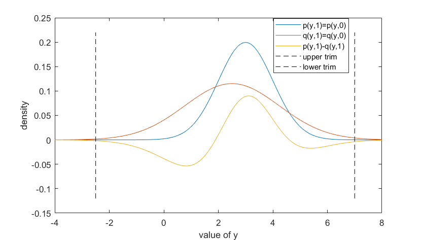
Refer to caption
Figure 2: Density of p⁡(y,d)p(y,d) and q⁡(y,d)q(y,d) of d∈{0,1}d\in\{0,1\}, and their difference.

The true identified value of L​A​T​EA~I​D​(F){LATE}^{ID}_{\tilde{A}}(F) is 1.73851.7385. Simulation results are given in Table 1. Coverage probability are calculated from 10001000 replications, and I compare the coverage probability under different sample size nn in each replication and the choice of trimming constant bb. The row of ‘known tail’ in Table 1 corresponds to the constraints 𝒴1u​t=𝒴1l​t=∅\mathcal{Y}^{ut}_{1}=\mathcal{Y}^{lt}_{1}=\varnothing, 𝒴0u​t=[Mu,∞)\mathcal{Y}^{ut}_{0}=[M_{u},\infty), and 𝒴0l​t=(−∞,Ml]\mathcal{Y}^{lt}_{0}=(-\infty,M_{l}] as in the simulation design. The row of ‘Conservative’ in Table 1 corresponds to the case that the tail set is unknown, and I take the union of confidence intervals under all 1616 possible tail conditions.

Table 1: Finite Sample Coverage Probability
α=0.05\alpha=0.05 n=1000 n=5000 n=5000
(b=0.02,h=0.4) (b=0.012,h=0.2) (b=0.0135,h=0.2)
Known Tail 0.965 0.963 0.935
Conservative 0.9825 0.988 0.975

The simulation result shows that if we can correctly impose the tail condition as in the known tail case, inference on the true LATE value based on (3.17) is asymptotically exact but can be sensitive to the choice of trimming sequence bnb_{n}. If we want to be agnostic about the true tail condition, the union method is conservative.

Simulation Setting II

When the IA-M assumption holds, by Vytlacil 2002, the potential outcome model is equivalent to the latent index model. In this simulation setting, let Ui∼U⁡[0,1]U_{i}\sim U[0,1] and Di=𝟙​(0.2+0.6​Zi>Ui)D_{i}=\mathbbm{1}(0.2+0.6Z_{i}>U_{i}), where U⁡[0,1]U[0,1] is a uniform distribution on interval [0,1][0,1], and Zi∼𝙱𝚎𝚛𝚗𝚘𝚞𝚕𝚕𝚒⁡(0.5)Z_{i}\sim\mathtt{Bernoulli}(0.5) is independent of UiU_{i}. The potential outcome (Yi​(1),Yi​(0))∼N⁡(μ,Σ)(Y_{i}(1),Y_{i}(0))\sim N(\mu,\Sigma), where μ=[2,1.5]\mu=[2,1.5] and V​a​r​(Yi​(1))=2Var(Y_{i}(1))=2, V​a​r​(Yi​(0))=1.5Var(Y_{i}(0))=1.5, C​o​r​r​(Yi​(1),Yi​(0))=0.7Corr(Y_{i}(1),Y_{i}(0))=0.7. We can show L​A​T​EI​D​(F)=0.5LATE^{ID}(F)=0.5.

Let L​A​T​E^W​a​l​d\widehat{LATE}^{Wald} denote the Wald estimator of L​A​T​EI​D​(F)LATE^{ID}(F), and let L​A​T​E^N​e​w\widehat{LATE}^{New} denote the estimator in equation (3.16). Table 2 shows some summary statistics of the numerical difference between these two estimators over m=1000m=1000 simulation replications. The first row shows that when the sample size increase, the numerical difference of the two estimator converges to zero in the second moment. The second row in Table 2 reports the efficiency loss of L​A​T​E^N​e​w\widehat{LATE}^{New}. We see that at finite sample, not imposing IA-M assumption when it holds can lead to efficiency loss, but the efficiency loss decreases with sample size.

Table 2: Monte Carlo simulation over 10001000 replications.
n=500n=500 n=1000n=1000 n=2500n=2500 n=5000n=5000
V​a​r​[L​A​T​E^W​a​l​d−L​A​T​E^N​e​w]Var\left[\widehat{LATE}^{Wald}-\widehat{LATE}^{New}\right] 0.0097 0.0031 0.0011 0.0004
σ⁡(L​A​T​E^N​e​w)−σ⁡(L​A​T​E^W​a​l​d)\sigma(\widehat{LATE}^{New})-\sigma(\widehat{LATE}^{Wald}) 0.020 .008 0.006 0.003
MSE(L​A​T​E^N​e​w\widehat{LATE}^{New})−-MSE(L​A​T​E^W​a​l​d\widehat{LATE}^{Wald}) 0.0082 0.0023 0.0011 0.0004

3.4 Empirical Illustration

In this section, I apply my results in Proposition 3.3 and Theorem 2 to Card 1993, who studied the causal effect of college attendance on earnings. In this application, the outcome variable YiY_{i} is an individual ii’s log wage in 1976, Di=1D_{i}=1 means individual ii attended a four-year college, and Zi=1Z_{i}=1 means the individual was born near a four-year college. This data set has been used by both Kitagawa 2015 and Mourifié and Wan 2017 to test the IA-M assumption, and they both reject the IA-M assumption. If a child grew up near a college, he or she may hear more stories of heavy tuition burden, which may discourage him or her from attending college. On the other hand, if this child grew up far away from a college, he or she may instead choose to attend college. Therefore, we would expect defiers to exist in this empirical setting. Moreover, it is unclear why this instrument is fully independent of the potential income, since the choice of residence may depend on parents’ potential income, which may be correlated with their children’s income.

I conditioned (Yi,Di,Zi)(Y_{i},D_{i},Z_{i}) on three characteristics: living in the south (S/NS), living in a metropolitan area (M/NM), and ethnic group (B/NB). I follow Mourifié and Wan 2017 in excluding subgroup NS/NM/B due to the small sample size, and also exclude subgroup NS/M/B due to the high frequency of Z=1Z=1. I conduct estimation and inference on each of the remaining 6 subgroups and the pooled sample. The choices of trimming sequence bnb_{n}, kernel bandwidth hh, upper and lower band Mu,MlM_{u},M_{l}, tail set 𝒴du​t,𝒴dl​t\mathcal{Y}_{d}^{ut},\mathcal{Y}_{d}^{lt} are specified in Appendix G.

Estimation results are reported in Table 3. I also report the LATE estimates when we directly use the IA-M assumption and Wald statistics. The estimated measure of compliers under A~\tilde{A} satisfying 3.1 conditioned on Zi=1Z_{i}=1 and Zi=0Z_{i}=0 are reported as P⁡(𝒴1,1)−Q⁡(𝒴1,1)P(\mathcal{Y}_{1},1)-Q(\mathcal{Y}_{1},1) and Q⁡(𝒴0,0)−P⁡(𝒴0,0)Q(\mathcal{Y}_{0},0)-P(\mathcal{Y}_{0},0), while the estimated measure of compliers under IA-M assumption is E⁡[Di|Zi=1]−E⁡[Di|Zi=0]E[D_{i}|Z_{i}=1]-E[D_{i}|Z_{i}=0]. The estimates of L​A​T​EA~I​D{LATE}^{ID}_{\tilde{A}} and L​A​T​EW​a​l​dLATE^{Wald} differ the most for three groups: S/NM/NB, S/M/NB and S/M/B. It should be noted that for all these three groups, estimated E⁡[Di|Zi=1]−E⁡[Di|Zi=0]E[D_{i}|Z_{i}=1]-E[D_{i}|Z_{i}=0] differs from P⁡(𝒴1,1)−Q⁡(𝒴1,1)P(\mathcal{Y}_{1},1)-Q(\mathcal{Y}_{1},1) and Q⁡(𝒴0,0)−P⁡(𝒴0,0)Q(\mathcal{Y}_{0},0)-P(\mathcal{Y}_{0},0). If we blindly use the identification result under the IA-M assumption and use the standard LATE Wald estimator, the ‘identified’ local average treatment effect can be negative (subgroups S/NM/NB and S/M/NB), or be unrealistically large (subgroup S/M/B). Once we use a strong extension, the estimated LATE for each of the 6 subgroups is positive, and the value of LATE is all between zero and one. We fail to reject education decrease future earning for the complier group (L​A​T​E<0LATE<0) for all 6 subgroups for the L​A​T​Ew​a​l​dLATE^{wald}. On the other hand, my method can reject the hypothesis L​A​T​E<0LATE<0 for the NS/NM/NB and the S/NM/B group at 95% confidence level. When I look at the African-American only, while L​A​T​Ew​a​l​dLATE^{wald} is large, the hypothesis fail to reject that education is harmful to their earning, while my method will reject the hypothesis L​A​T​Ew​a​l​dLATE^{wald} for the African-American is negative.

Table 3: Estimation Result under Extensions Assumption 3.1
Group NS,NM,NB NS,M,NB S,NM,NB S,NM,B S,M,NB S,M,B B-Group Only
P​r​(Zi=1)Pr(Z_{i}=1) 0.464 0.879 0.349 0.322 0.608 0.802 0.6188
Observations 429 1191 307 314 380 246 703
L​A​T​EA~I​D​(F)LATE^{ID}_{\tilde{A}}(F) 0.5599 0.1546 0.2524 0.4773 0.5276 0.4358 1.0993
CI for L​A​T​EA~I​D​(F)LATE^{ID}_{\tilde{A}}(F) [0.01, 1.11] [-0.51, 0.82] [-1.22, 1.73] [-0.09,1.04] [-2.54, 3.59] [-5.15, 6.02] [0.58, 1.62]
P⁡(𝒴1,1)−Q⁡(𝒴1,1)P(\mathcal{Y}_{1},1)-Q(\mathcal{Y}_{1},1) 0.1120 0.1084 0.0265 0.0739 0.0164 0.0338 0.0375
Q⁡(𝒴0,0)−P⁡(𝒴0,0)Q(\mathcal{Y}_{0},0)-P(\mathcal{Y}_{0},0) 0.1148 0.0960 0.0684 0.1495 0.0922 0.0308 0.1583
L​A​T​Ew​a​l​d​(F)LATE^{wald}(F) 0.5976 0.0761 -6.4251 1.1873 -1.5412 17.9620 5.0499
CI for L​A​T​Ew​a​l​d​(F){LATE}^{wald}(F) [-0.20 1.39] [-1.24, 1.39] [-105,92] [-0.53,2.90] [-5.09,2.01] [-1.7e4,1.7e4] [-6.16,16.26]
E⁡[Di|Zi=1]E[D_{i}|Z_{i}=1]
-E⁡[Di|Zi=0]E[D_{i}|Z_{i}=0]
0.1080 0.1084 -0.0070 0.0692 -0.0697 0.0002 0.0317

4 Application to Binary Outcome Sector Choice

In this section, I apply the method to a binary outcome sector choice model with a binary instrument (Mourifie et al. 2018). This model is incomplete. Observed outcome Yi∈{0,1}Y_{i}\in\{0,1\} is binary and the observed job sector choice Di∈{0,1}D_{i}\in\{0,1\} is binary. A binary instrument ZiZ_{i} is observed. The ϵ\epsilon variables include Yi​(1)Y_{i}(1) and Yi​(0)Y_{i}(0), which are the potential outcome in job sector 1 and 0 respectively, and the instrument variable ZiZ_{i}. Observed sector outcome YiY_{i} is generated through:

Yi=Yi​(1)​Di+Yi​(0)​(1−Di).Y_{i}=Y_{i}(1)D_{i}+Y_{i}(0)(1-D_{i}). (4.1)

Without imposing further assumptions, equation (4.1) does not specify how sector choice DiD_{i} is determined, and DiD_{i} can take values in one of the three sets {0},{1},{0,1}\{0\},\{1\},\{0,1\}. If we impose the classical Roy sector selection rule, for all Zi=z∈{0,1}Z_{i}=z\in\{0,1\} we have:

Di∈{{1}i​fYi​(1)>Yi​(0),{0}i​fYi​(0)<Yi​(1),{0,1}i​fYi​(1)=Yi​(0).D_{i}\in\begin{cases}\{1\}\quad&if\quad Y_{i}(1)>Y_{i}(0),\\ \{0\}\quad&if\quad Y_{i}(0)<Y_{i}(1),\\ \{0,1\}\quad&if\quad Y_{i}(1)=Y_{i}(0).\end{cases} (4.2)

The Roy sector selection rule (4.2) is just a special case of how DiD_{i} is determined. To specify the structure universe 𝒮\mathcal{S}, we consider all possible sector selection rules. 1010 10 For each Yi​(0)=y0,Yi​(1)=y1,Zi=zY_{i}(0)=y_{0},Y_{i}(1)=y_{1},Z_{i}=z, DiD_{i} can take values in three sets {0},{1},{0,1}\{0\},\{1\},\{0,1\}. Therefore, there are 383^{8} ways to specify the sector selection rule.

Definition 4.1.

A sector selection rule is a set-valued function

Ds​e​l:{0,1}3→{{0},{1},{0,1}},(y1,y0,z)→Ds​e​l​(y1,y0,z).\begin{split}D^{sel}:\{0,1\}^{3}&\rightarrow\{\{0\},\{1\},\{0,1\}\},\\ (y_{1},y_{0},z)&\rightarrow D^{sel}(y_{1},y_{0},z).\end{split}

Let 𝒟s​e​l\mathcal{D}^{sel} be the collection of all possible sector selection rules. Let Ds,s​e​l∈𝒟s​e​lD^{s,sel}\in\mathcal{D}^{sel} be a sector selection rule. Given a distribution Gs​(ϵ)G^{s}(\epsilon) and a Ds,s​e​lD^{s,sel}, the associated correspondence MsM^{s} is defined as:

Ms(Gs)≡{F∈ℱ:P​rF​(Yi=y,Di=d,Zi=z)=(C1y​0​z+C1y​1​z)​𝟙​(d=1)+(C00​y​z+C01​y​z)​𝟙​(d=0),holds for some vector​(Cdy​k​z)y,k,z,d∈{0,1}​ such that C1y​k​z+C0y​k​z=P​rGs​(Yi​(1)=y,Yi​(0)=k,Zi=z),Cy​k​zd=0ifDs,s​e​l(y,k,z)={1−d}andCy​k​zd≥0∀y,k,z,d∈{0,1}}.\begin{split}M^{s}(G^{s})\equiv\bigg\{F\in\mathcal{F}:&Pr_{F}(Y_{i}=y,D_{i}=d,Z_{i}=z)=(C^{y0z}_{1}+C^{y1z}_{1})\mathbbm{1}(d=1)+(C^{0yz}_{0}+C^{1yz}_{0})\mathbbm{1}(d=0),\\ &\text{holds for some vector}\left(C^{ykz}_{d}\right)_{y,k,z,d\in\{0,1\}}\text{ such that }\\ &C^{ykz}_{1}+C^{ykz}_{0}=Pr_{G^{s}}(Y_{i}(1)=y,Y_{i}(0)=k,Z_{i}=z),\\ &C^{ykz}_{d}=0\hskip 8.50012ptif\hskip 8.50012ptD^{s,sel}(y,k,z)=\{1-d\}\hskip 8.50012ptand\hskip 8.50012ptC^{ykz}_{d}\geq 0\hskip 8.50012pt\hskip 8.50012pt\forall y,k,z,d\in\{0,1\}\bigg\}.\end{split} (4.3)

In Definition 4.1, Cdy​k​zC^{ykz}_{d} is the probability of choosing sector dd when Yi​(1)=y,Yi​(0)=k,Zi=zY_{i}(1)=y,Y_{i}(0)=k,Z_{i}=z. When Ds,s​e​l​(y,k,z)D^{s,sel}(y,k,z) is the set {0,1}\{0,1\}, a structure ss associated with Ds,s​e​lD^{s,sel} does not specify how a sector choice is determined, so the only constraint is C1y​k​z+C0y​k​z=P​rGs​(Yi​(1)=y,Yi​(1)=k,Zi=z)C^{ykz}_{1}+C^{ykz}_{0}=Pr_{G^{s}}(Y_{i}(1)=y,Y_{i}(1)=k,Z_{i}=z). When Ds,s​e​l​(y,k,z)={d}D^{s,sel}(y,k,z)=\{d\}, the constraint C1−dy​k​z=0C^{ykz}_{1-d}=0 in the last row of (4.3) requires the probability of choosing sector 1−d1-d is zero. Given the set of sector selection rules 𝒟s​e​l\mathcal{D}^{sel}, we can specify the structure universe 𝒮\mathcal{S} in this application as follows:

𝒮={s=(Ms,Gs)|Gsis a distribution of (Yi(1),Yi(0),Zi),Msis associated with a Ds​e​l∈𝒟s,s​e​l}.\begin{split}\mathcal{S}=\bigg\{s=(M^{s},G^{s})\bigg|&G^{s}\,\,\text{is a distribution of }(Y_{i}(1),Y_{i}(0),Z_{i}),\quad\\ &M^{s}\,\,\text{is associated with a }D^{sel}\in\mathcal{D}^{s,sel}\bigg\}.\end{split} (4.4)

Instead of imposing the strong independent instrument condition (Yi​(1),Yi​(0))⟂Zi\left(Y_{i}(1),Y_{i}(0)\right)\perp Z_{i}, we require the instrument to have monotone effects on the potential outcomes:

Definition 4.2.

We say (Yi​(1),Yi​(0))|Zi=1(Y_{i}(1),Y_{i}(0))|Z_{i}=1 dominates (Yi​(1),Yi​(0))|Zi=0(Y_{i}(1),Y_{i}(0))|Z_{i}=0 at the best and worst outcomes if

P​r​(Yi​(1)=Yi​(0)=1|Zi=1)≥P​r​(Yi​(1)=Yi​(0)=1|Zi=0),P​r​(Yi​(1)=Yi​(0)=0|Zi=1)≤P​r​(Yi​(1)=Yi​(0)=0|Zi=0).\begin{split}Pr(Y_{i}(1)=Y_{i}(0)=1|Z_{i}=1)&\geq Pr(Y_{i}(1)=Y_{i}(0)=1|Z_{i}=0),\\ Pr(Y_{i}(1)=Y_{i}(0)=0|Z_{i}=1)&\leq Pr(Y_{i}(1)=Y_{i}(0)=0|Z_{i}=0).\end{split} (4.5)

Definition 4.2 only requires the instrument to generate the best (resp. worst) potential outcome Yi​(1)=Yi​(0)=1Y_{i}(1)=Y_{i}(0)=1 (resp. Yi​(1)=Yi​(0)=0Y_{i}(1)=Y_{i}(0)=0) with higher (resp. lower) probability at Zi=1Z_{i}=1 than that at Zi=0Z_{i}=0. This requirement is weaker than Assumption 5 in (Mourifie et al. 2018), where they require P​r​(Yi​(d)=1|Zi=1)≥P​r​(Yi​(d)=1|Zi=0)Pr(Y_{i}(d)=1|Z_{i}=1)\geq Pr(Y_{i}(d)=1|Z_{i}=0) for d∈{0,1}d\in\{0,1\} in addition to (4.5). 1111 11 Condition (4.5) along with the additional requirement P​r​(Yi​(1)=1|Zi=1)≥P​r​(Yi​(1)=1|Zi=0)Pr(Y_{i}(1)=1|Z_{i}=1)\geq Pr(Y_{i}(1)=1|Z_{i}=0) will imply 1−P​rF​(Yi=0,Di=1|Zi=1)≥P​rF​(Yi=1,Di=1|Zi=0)1-Pr_{F}(Y_{i}=0,D_{i}=1|Z_{i}=1)\geq Pr_{F}(Y_{i}=1,D_{i}=1|Z_{i}=0) for all outcome distributions FF. This implication holds even in the absence of the Roy selection condition. On the other hand, equation (4.5) alone does not imply any constraints on FF.

Dominance at the best and worst outcome in Definition 4.2 can accommodate broader empirical scenarios compared with Assumption 5 in (Mourifie et al. 2018). For example, suppose Yi​(d)=1Y_{i}(d)=1 means individual ii gets tenure in sector dd, and Zi=1Z_{i}=1 means individual ii participates in a job training program. If the skill obtained from the training program can be applied to both sectors, we would expect P​r​(Yi​(1)=Yi​(0)=1|Zi=1)≥P​r​(Yi​(1)=Yi​(0)=1|Zi=0)Pr(Y_{i}(1)=Y_{i}(0)=1|Z_{i}=1)\geq Pr(Y_{i}(1)=Y_{i}(0)=1|Z_{i}=0). On the other hand, each job sector may require specific skill that cannot be obtained from the job training program. If the training program is costly and prevents an individual ii from developing skills specific to the sector dd, it is possible that P​r​(Yi​(d)=1|Zi=1)≤P​r​(Yi​(d)=1|Zi=0)Pr(Y_{i}(d)=1|Z_{i}=1)\leq Pr(Y_{i}(d)=1|Z_{i}=0). Such a scenario violates Assumption 5 in Mourifie et al. 2018 but not (4.5). Lastly, P​r​(Yi​(1)=Yi​(0)=0|Zi=1)≤P​r​(Yi​(1)=Yi​(0)=0|Zi=0)Pr(Y_{i}(1)=Y_{i}(0)=0|Z_{i}=1)\leq Pr(Y_{i}(1)=Y_{i}(0)=0|Z_{i}=0) ensures the training program is beneficial: it increases the probability of success in at least one sector.

However, when (4.5) is combined with Roy’s selection assumption, they are jointly refutable. Formally, the assumption with Roy’s selection rule and a monotone instrument satisfying (4.5) is defined in the following.

Assumption 4.1.

The assumption of Roy’s selection rule with instrument condition (4.5), denoted as AR​o​yA^{Roy}, is the collection of structures such that

AR​o​y={s∈𝒮:Ms​is associated with the ​Ds​e​l​in​(4.2),Ms(Gs)satisfies(4.3),Gssatisfies(4.5)}.\begin{split}A^{Roy}=\bigg\{s\in\mathcal{S}:\,\,&M^{s}\,\,\text{is associated with the }\,\,D^{sel}\,\,\text{in}\,\,(\ref{eq: roy model, perfect selection D_i mapping}),\\ &M^{s}(G^{s})\,\,\text{satisfies}(\ref{eq: Roy appli, M^s}),\quad G^{s}\,\,\text{satisfies}(\ref{eq: roy model, dominating instrument at best and worst outcome})\bigg\}.\end{split} (4.6)

The following proposition characterizes the non-refutability and confirmation sets associated with AR​o​yA^{Roy}.

Proposition 4.1.

Let ℱn​f\mathcal{F}^{nf} be the collection of outcome distributions such that

P​rF​(Yi=0|Zi=1)≤P​rF​(Yi=0|Zi=0).\begin{split}Pr_{F}(Y_{i}=0|Z_{i}=1)\leq Pr_{F}(Y_{i}=0|Z_{i}=0).\end{split} (4.7)

The non-refutability and confirmation sets of AR​o​yA^{Roy} are

ℋ𝒮s​n​f​(AR​o​y)={s:Ms​(Gs)⊆ℱn​f},ℋ𝒮w​n​f​(AR​o​y)={s:Ms​(Gs)∩ℱn​f≠∅},ℋ𝒮s​c​o​n​(AR​o​y)=ℋ𝒮w​c​o​n​(AR​o​y)=∅.\begin{split}\mathcal{H}_{\mathcal{S}}^{snf}(A^{Roy})&=\{s:\,M^{s}(G^{s})\subseteq\mathcal{F}^{nf}\},\\ \mathcal{H}_{\mathcal{S}}^{wnf}(A^{Roy})&=\{s:\,M^{s}(G^{s})\cap\mathcal{F}^{nf}\neq\varnothing\},\\ \mathcal{H}_{\mathcal{S}}^{scon}(A^{Roy})&=\mathcal{H}_{\mathcal{S}}^{wcon}(A^{Roy})=\varnothing.\end{split}

Proposition 4.1 reveals several things: first ℋ𝒮s​n​f​(AR​o​y)≠𝒮\mathcal{H}_{\mathcal{S}}^{snf}(A^{Roy})\neq\mathcal{S}, so the assumption AR​o​yA^{Roy} is refutable; second, ℋ𝒮w​n​f​(AR​o​y)≠ℋ𝒮s​n​f​(AR​o​y)\mathcal{H}_{\mathcal{S}}^{wnf}(A^{Roy})\neq\mathcal{H}_{\mathcal{S}}^{snf}(A^{Roy}) so we cannot find a strong extension of AR​o​yA^{Roy}. Therefore, I look at the completion of the binary sector choice model. The completion given in Definition 2.12 is abstract and in the following I give an explicit form of 𝒞⁡(s)\mathcal{C}(s).

Recall that each ss in the incomplete space is associated with a sector decision rule, denoted by Ds,s​e​lD^{s,sel}. We consider a tie breaking rule associated with ss: (Cds∗,t​b​(y,k,z))y,k,z,d∈{0,1}\left(C^{s^{*},tb}_{d}(y,k,z)\right)_{y,k,z,d\in\{0,1\}}, which specifies the probability of choosing sector dd for different values of Yi​(0)=y,Yi​(1)=k,Zi=zY_{i}(0)=y,Y_{i}(1)=k,Z_{i}=z. Different values of the vector (Cds∗,t​b​(y,k,z))y,k,z,d∈{0,1}\left(C^{s^{*},tb}_{d}(y,k,z)\right)_{y,k,z,d\in\{0,1\}} correspond to different selections. The completion 𝒞⁡(s)\mathcal{C}(s) is the collection of Ms∗​(⋅)M^{s^{*}}(\cdot) such that

Ms∗(Gs)={F∈ℱ|∀y,k,z,d∈{0,1}:Cdy​k​z=Cds∗,t​b​(y,k,z)×P​rGs​(Yi​(1)=y,Yi​(0)=k,Zi=z),P​rF​(Yi=y,Di=d,Zi=z)=(Cdy​0​z+Cdy​1​z)​𝟙​(d=1)+(Cd0​y​z+Cd1​y​z)​𝟙​(d=0)holds for a vector ​(Cds∗,t​b​(y,k,z))y,k,z,d∈{0,1}​ such that ∑d=01Cs∗,t​bd(y,k,z)≡1,Cs∗,t​bd(y,k,z)=1 if Ds,s​e​l(y,k,z)={d}}.\begin{split}M^{s^{*}}(G^{s})=\bigg\{&F\in\mathcal{F}\bigg|\forall y,k,z,d\in\{0,1\}:C^{ykz}_{d}=C^{s^{*},tb}_{d}(y,k,z)\times Pr_{G^{s}}(Y_{i}(1)=y,Y_{i}(0)=k,Z_{i}=z),\\ &Pr_{F}(Y_{i}=y,D_{i}=d,Z_{i}=z)=(C^{y0z}_{d}+C^{y1z}_{d})\mathbbm{1}(d=1)+(C^{0yz}_{d}+C^{1yz}_{d})\mathbbm{1}(d=0)\\ &\text{holds for a vector }\left(C^{s^{*},tb}_{d}(y,k,z)\right)_{y,k,z,d\in\{0,1\}}\text{ such that }\\ &\sum_{d=0}^{1}C^{s^{*},tb}_{d}(y,k,z)\equiv 1,\quad C^{s^{*},tb}_{d}(y,k,z)=1\text{ if }D^{s,sel}(y,k,z)=\{d\}\bigg\}.\end{split} (4.8)

Compared with the incomplete mapping in (4.3), the tie breaking rule Cds∗,t​bC_{d}^{s^{*},tb} makes Ms∗​(Gs)M^{s^{*}}(G^{s}) a singleton. The completed universe is given in Definition 2.12 and the corresponding Roy assumption set in the completed structural universe is given in Definition Proposition 2.8.

Minimal Efficiency Loss and the Corresponding Strong Extension

I now consider a strong extension under the completed structure universe 𝒮∗\mathcal{S}^{*}. I first define the efficiency loss of a structure s∗s^{*}, which can be viewed as a deviation from Roy’s sector selection assumption.

Definition 4.3.

The efficiency loss of a structure s∗∈𝒮∗s^{*}\in\mathcal{S}^{*}

mE​L​(s∗)=EGs∗​[max⁡{Yi​(1),Yi​(0)}]−EF​[Yi]f​o​rF∈Ms∗​(Gs∗)m^{EL}(s^{*})=E_{G^{s^{*}}}[\max\{Y_{i}(1),Y_{i}(0)\}]-E_{F}[Y_{i}]\quad\quad for\quad F\in M^{s^{*}}(G^{s^{*}}) (4.9)

is the difference between the expected optimal sector selection outcome and the expected predicted outcome.

The efficiency loss is a function since Ms∗​(Gs∗)M^{s^{*}}(G^{s^{*}}) is a singleton. It is easy to see that when the Roy sector selection rule holds, mE​L​(s∗)=0m^{EL}(s^{*})=0. Conversely, by (4.1), mE​L​(s∗)=0m^{EL}(s^{*})=0 implies

Di={1ifYi​(1)>Yi​(0)0ifYi​(1)<Yi​(0)D_{i}=\begin{cases}1\quad\quad\text{if}\quad Y_{i}(1)>Y_{i}(0)\\ 0\quad\quad\text{if}\quad Y_{i}(1)<Y_{i}(0)\\ \end{cases}

with probability 1, so the Roy sector selection rule holds. Once we verify mE​L​(s∗)m^{EL}(s^{*}) is a well-behaved minimal deviation measure (see Definition 2.10), we can use minimal efficiency loss to construct a strong extension.

Assumption 4.2.

Let mm​i​n​(F)≡inf{mE​L​(s∗):F∈Ms∗​(Gs∗)​a​n​d​Gs∗​ satisfies ​(4.5)}m^{min}(F)\equiv\inf\{m^{EL}(s^{*}):F\in M^{s^{*}}(G^{s^{*}})\,\,and\,\,G^{s^{*}}\text{ satisfies }(\ref{eq: roy model, dominating instrument at best and worst outcome})\} be the minimal efficiency loss under FF. We call

A~=∪F∈ℱ{s∗:mE​L(s∗)=mm​i​n(F),Gs∗ satisfies (4.5)}\tilde{A}=\cup_{F\in\mathcal{F}}\left\{s^{*}:m^{EL}(s^{*})=m^{min}(F),\,G^{s^{*}}\text{ satisfies }(\ref{eq: roy model, dominating instrument at best and worst outcome})\right\}

the minimal efficiency loss extension of AR​o​yA^{Roy}.

Proposition 4.2.

A~∗R​o​y\tilde{A}^{*Roy} is a strong extension of A∗R​o​yA^{*Roy}. Moreover, given an observed distribution FF, the identified set for Gs∗G^{s^{*}} under A~∗R​o​y\tilde{A}^{*Roy} is

{Gs∗| there exists ​{Cdy​k​z}​∀y,k,z,d∈{0,1}​s.t.Cdy​k​z≥0,P​rF​(Yi=y,Di=d,Zi=z)=(Cdy​0​z+Cdy​1​z)​𝟙​(d=1)+(Cd0​y​z+Cd1​y​z)​𝟙​(d=0),Cy​k​z1+Cy​k​z0=PrGs∗(Yi(1)=y,Yi(0)=k,Zi=z),C0101=C1000=0,C1110+C0110P​rF​(Zi=0)≤C1111+C0111P​rF​(Zi=1),C1010+C0111=max{PrF(Yi=0,Zi=1)−P​rF​(Yi=0,Zi=0)​P​rF​(Zi=1)P​rF​(Zi=0),0}}.\begin{split}\Bigg\{G^{s^{*}}\bigg|&\text{ there exists }\{C_{d}^{ykz}\}\hskip 8.50012pt\forall{y,k,z,d\in\{0,1\}}\,\,s.t.\,\,C_{d}^{ykz}\geq 0,\\ &Pr_{F}(Y_{i}=y,D_{i}=d,Z_{i}=z)=(C^{y0z}_{d}+C^{y1z}_{d})\mathbbm{1}(d=1)+(C^{0yz}_{d}+C^{1yz}_{d})\mathbbm{1}(d=0),\\ &C^{ykz}_{1}+C^{ykz}_{0}=Pr_{G^{s*}}(Y_{i}(1)=y,Y_{i}(0)=k,Z_{i}=z),\\ &C^{010}_{1}=C^{100}_{0}=0,\hskip 8.50012pt\frac{C^{110}_{1}+C^{110}_{0}}{Pr_{F}(Z_{i}=0)}\leq\frac{C^{111}_{1}+C^{111}_{0}}{Pr_{F}(Z_{i}=1)},\\ &C^{101}_{0}+C^{011}_{1}=\max\left\{Pr_{F}(Y_{i}=0,Z_{i}=1)-\frac{Pr_{F}(Y_{i}=0,Z_{i}=0)Pr_{F}(Z_{i}=1)}{Pr_{F}(Z_{i}=0)},0\right\}\Bigg\}.\end{split} (4.10)

Proposition 4.2 characterizes the sharp identified set of distributions of (Yi​(1),Yi​(0),Zi)(Y_{i}(1),Y_{i}(0),Z_{i}). The identified set (4.10) under A~∗R​o​y\tilde{A}^{*Roy} satisfies: (1). There is no efficiency loss when Zi=0Z_{i}=0 (C1010=C0100=0C^{010}_{1}=C^{100}_{0}=0); (2). The minimal efficiency loss is max⁡{P​rF​(Yi=0,Zi=1)−P​rF​(Yi=0,Zi=0)​P​rF​(Zi=1)P​rF​(Zi=0),0}\max\left\{Pr_{F}(Y_{i}=0,Z_{i}=1)-\frac{Pr_{F}(Y_{i}=0,Z_{i}=0)Pr_{F}(Z_{i}=1)}{Pr_{F}(Z_{i}=0)},0\right\}; (3). Condition (4.5) holds as long as (C1110+C0110)​P​rF​(Zi=1)≤(C1111+C0111)​P​rF​(Zi=0)(C^{110}_{1}+C^{110}_{0}){Pr_{F}(Z_{i}=1)}\leq(C^{111}_{1}+C^{111}_{0}){Pr_{F}(Z_{i}=0)} holds. The identified set of Gs∗G^{s^{*}} is a polyhedron characterized by the 16-dimensional vector (Cdy​k​z)y,k,z,d∈{0,1}(C_{d}^{ykz})_{y,k,z,d\in\{0,1\}}. Many parameters of interest are linear functions of (Cdj​k​z)(C^{jkz}_{d}), and linear-programming can be used to find the identified set. One example is given in Corollary 4.1.

Corollary 4.1.

The identified set for P​r​(Yi​(1)=1|Zi=z)Pr(Y_{i}(1)=1|Z_{i}=z) under A~∗R​o​y\tilde{A}^{*Roy} is

P​r​(Yi=1,Di=1|Zi=0)≤P​r​(Yi​(1)=1|Zi=0)≤P​r​(Yi=1|Zi=0),P​r​(Yi=1,Di=1|Zi=1)≤P​r​(Yi​(1)=1|Zi=1)≤P​r​(Yi=1|Zi=1)+mE​L,m​i​n​(F)P​r​(Zi=1),\begin{split}Pr(Y_{i}=1,D_{i}=1|Z_{i}=0)\leq&Pr(Y_{i}(1)=1|Z_{i}=0)\leq Pr(Y_{i}=1|Z_{i}=0),\\ Pr(Y_{i}=1,D_{i}=1|Z_{i}=1)\leq&Pr(Y_{i}(1)=1|Z_{i}=1)\leq Pr(Y_{i}=1|Z_{i}=1)+\frac{m^{EL,min}(F)}{Pr(Z_{i}=1)},\\ \end{split}

where mE​L,m​i​n​(F)=max⁡{P​rF​(Yi=0,Zi=1)−P​rF​(Yi=0,Zi=0)​P​rF​(Zi=1)P​rF​(Zi=0),0}m^{EL,min}(F)=\max\left\{Pr_{F}(Y_{i}=0,Z_{i}=1)-\frac{Pr_{F}(Y_{i}=0,Z_{i}=0)Pr_{F}(Z_{i}=1)}{Pr_{F}(Z_{i}=0)},0\right\}.

It is worth noticing that if A∗R​o​yA^{*Roy} cannot be rejected by FF, the identified set for θ≡P​r​(Yi​(1)=1|Zi=1)\theta\equiv Pr(Y_{i}(1)=1|Z_{i}=1) is given by [P​r​(Yi=1,Di=1|Zi=1),P​r​(Yi=1|Zi=1)][Pr(Y_{i}=1,D_{i}=1|Z_{i}=1),Pr(Y_{i}=1|Z_{i}=1)]. However, suppose we ignore the testable implication of A∗R​o​yA^{*Roy} and directly use [P​r​(Yi=1,Di=1|Zi=1),P​r​(Yi=1|Zi=1)][Pr(Y_{i}=1,D_{i}=1|Z_{i}=1),Pr(Y_{i}=1|Z_{i}=1)] as the identified set for θ\theta, we get a spuriously informative identified set when mE​L,m​i​n​(F)>0m^{EL,min}(F)>0. This happens when the true structure that generates the data lies in A~∗R​o​y\A∗R​o​y\tilde{A}^{*Roy}\backslash{A}^{*Roy}, and the spuriously informative identified set is a proper subset of the true identified set.

The upper bound of the identified set for P​r​(Yi​(1)=1|Zi=1)Pr(Y_{i}(1)=1|Z_{i}=1) is not Fréchet differentiable with respect to FF due to the max\max operator. However, by Example 2 in Fang and Santos 2019, the upper bound P​r​(Yi=1|Zi=1)+mE​L,m​i​n​(F)P​r​(Zi=1)Pr(Y_{i}=1|Z_{i}=1)+\frac{m^{EL,min}(F)}{Pr(Z_{i}=1)} is directionally differentiable in FF. The bootstrap method in Fang and Santos 2019 can be used to construct confidence interval for P​r​(Yi​(1)=1|Zi=1)Pr(Y_{i}(1)=1|Z_{i}=1). However, since P​r​(Yi​(1)=1|Zi=1)Pr(Y_{i}(1)=1|Z_{i}=1) is partially identified and satisfies the conditions in Proposition 2.11, we cannot directly test a hypothesis on the value of P​r​(Yi​(1)=1|Zi=1)Pr(Y_{i}(1)=1|Z_{i}=1). Instead, we should test the equivalent existence hypothesis as in Proposition 2.13.

References

  • Bonhomme and Weidner (2018) Bonhomme, S. and M. Weidner (2018). Minimizing sensitivity to model misspecification. arXiv preprint arXiv:1807.02161.
  • Bresnahan and Reiss (1991) Bresnahan, T. F. and P. C. Reiss (1991). Empirical models of discrete games. Journal of Econometrics 48(1-2), 57–81.
  • Breusch (1986) Breusch, T. S. (1986). Hypothesis testing in unidentified models. The Review of Economic Studies 53(4), 635–651.
  • Card (1993) Card, D. (1993). Using geographic variation in college proximity to estimate the return to schooling.
  • Chesher and Rosen (2012) Chesher, A. and A. M. Rosen (2012). Simultaneous equations models for discrete outcomes: coherence, completeness, and identification. Technical report, cemmap working paper.
  • Christensen and Connault (2019) Christensen, T. and B. Connault (2019). Counterfactual sensitivity and robustness. arXiv preprint arXiv:1904.00989.
  • De Chaisemartin (2017) De Chaisemartin, C. (2017). Tolerating defiance? local average treatment effects without monotonicity. Quantitative Economics 8(2), 367–396.
  • Fang and Santos (2019) Fang, Z. and A. Santos (2019). Inference on directionally differentiable functions. The Review of Economic Studies 86(1), 377–412.
  • Galichon and Henry (2011) Galichon, A. and M. Henry (2011). Set identification in models with multiple equilibria. The Review of Economic Studies 78(4), 1264–1298.
  • Galichon and Henry (2013) Galichon, A. and M. Henry (2013). Dilation bootstrap. Journal of Econometrics 177(1), 109–115.
  • Hansen and Sargent (2007) Hansen, L. P. and T. J. Sargent (2007). Recursive robust estimation and control without commitment. Journal of Economic Theory 136(1), 1–27.
  • Hansen et al. (2006) Hansen, L. P., T. J. Sargent, G. Turmuhambetova, and N. Williams (2006). Robust control and model misspecification. Journal of Economic Theory 128(1), 45–90.
  • Imbens and Angrist (1994) Imbens, G. and J. Angrist (1994). Identification and estimation of local average treatment effects. Econometrica 62(2).
  • Jovanovic (1989) Jovanovic, B. (1989). Observable implications of models with multiple equilibria. Econometrica: Journal of the Econometric Society, 1431–1437.
  • Kedagni (2019) Kedagni, D. (2019). Identification of treatment effects with mismeasured imperfect instruments. Available at SSRN 3388373.
  • Kitagawa (2009) Kitagawa, T. (2009). Identification region of the potential outcome distributions under instrument independence. Working Paper.
  • Kitagawa (2015) Kitagawa, T. (2015). A test for instrument validity. Econometrica 83(5), 2043–2063.
  • Koopmans and Reiersol (1950) Koopmans, T. C. and O. Reiersol (1950). The identification of structural characteristics. The Annals of Mathematical Statistics 21(2), 165–181.
  • Manski (2019) Manski, C. F. (2019). Econometrics for decision making: Building foundations sketched by haavelmo and wald.
  • Manski and Tetenov (2020) Manski, C. F. and A. Tetenov (2020). Statistical decision properties of imprecise trials assessing covid-19 drugs.
  • Masten and Poirier (2018) Masten, M. and A. Poirier (2018). Salvaging falsified instrumental variable models. Working Paper.
  • Mourifie et al. (2018) Mourifie, I., M. Henry, and R. Méango (2018). Sharp bounds and testability of a roy model of stem major choices. Available at SSRN 2043117.
  • Mourifié and Wan (2017) Mourifié, I. and Y. Wan (2017). Testing local average treatment effect assumptions. Review of Economics and Statistics 99(2), 305–313.
  • Roy (1951) Roy, A. D. (1951). Some thoughts on the distribution of earnings. Oxford economic papers 3(2), 135–146.
  • Tamer (2003) Tamer, E. (2003). Incomplete simultaneous discrete response model with multiple equilibria. The Review of Economic Studies 70(1), 147–165.
  • Vytlacil (2002) Vytlacil, E. (2002). Independence, monotonicity, and latent index models: An equivalence result. Econometrica 70(1), 331–341.

Appendix A Discussion of Property 1

When the structure universe 𝒮\mathcal{S} is complete, the following proposition provides sufficient high level conditions to check whether ΘA~I​D\Theta_{\tilde{A}}^{ID} is a continuous correspondence in FF.

Proposition A.1.

Let (ℱ,dF)(\mathcal{F},d_{F}) and (Θ,dθ)(\Theta,d_{\theta}) be metric spaces, and let 𝒮\mathcal{S} be a complete structure universe. Let τℱ\tau_{\mathcal{F}} be the topology on ℱ\mathcal{F} induced by dFd_{F}. Let A=Aj∩(∩l≠jAl)A=A_{j}\cap(\cap_{l\neq j}A_{l}), and let jj be the index, mjm_{j} be the well-defined relaxation measure in Definition 2.11. We equip the ∩l≠jAl\cap_{l\neq j}A_{l} space with the weak topology τA−j\tau_{A_{-j}} induced by the mapping h⁡(s)=Ms​(Gs)h(s)=M^{s}(G^{s}) 1212 12 This is a slight abuse of the notation since h⁡(s)h(s) is a single-valued correspondence and its image space is 2ℱ2^{\mathcal{F}}. I abuse the notation and use h⁡(s)h(s) to denote the Ms​(Gs)M^{s}(G^{s}) mapping composited with the unique selection from the image set Ms​(Gs)M^{s}(G^{s}). :

τA−j≡{O⊂∩l≠jAl:O=h−1(P)∩(∩l≠jAl)forsomeP∈τℱ}.\tau_{A_{-j}}\equiv\{O\subset\cap_{l\neq j}A_{l}:\,O=h^{-1}(P)\cap(\cap_{l\neq j}A_{l})\,\,for\,\,some\,\,P\in\tau_{\mathcal{F}}\}.

Suppose: (1) θ(s):∩l≠jAl→Θ\theta(s):\cap_{l\neq j}A_{l}\rightarrow\Theta is a continuous function; and (2) the function

min(F;mj)≡inf{mj(s):F∈Ms(Gs)ands∈∩l≠jAl}\min(F;m_{j})\equiv\inf\{m_{j}(s):F\in M^{s}(G^{s})\quad and\quad s\in\cap_{l\neq j}A_{l}\}

is a continuous mapping from ℱ\mathcal{F} to ℝ\mathbb{R}. If mj−1:ℝ⇉∩l≠jAlm_{j}^{-1}:\mathbb{R}\rightrightarrows\cap_{l\neq j}A_{l} is an upper (resp. lower) hemicontinuous correspondence, then ΘA~I​D​(F)\Theta^{ID}_{\tilde{A}}(F) is an upper (resp. lower) hemicontinuous correspondence from (ℱ,dF)(\mathcal{F},d_{F}) to (Θ,dθ)(\Theta,d_{\theta}).

Proof.

See Online Appendix F.2. ∎

Here is a reasoning behind Property 1: We may want a continuous relation between the structure universe 𝒮\mathcal{S} and the observation space ℱ\mathcal{F}. When the true structure ss change a little, the predicted observation distribution should not change drastically. Similarly, the parameter of interest θ\theta should also be continuous with respect to change in the true structure. The relation can be represented as ℱ←Ms​(Gs)𝒮→θ⁡(s)Θ\mathcal{F}\xleftarrow{M^{s}(G^{s})}\mathcal{S}\xrightarrow{\,\,\theta(s)\,\,}\Theta. Unfortunately, there may not exist a natural topology embedded in 𝒮\mathcal{S}. The weak topology defined in Proposition A.1 is the smallest topology such that the mapping Ms​(Gs)M^{s}(G^{s}) is continuous. The construction of τA−j\tau_{A_{-j}} in Proposition A.1 uses the inverse of Ms​(Gs)M^{s}(G^{s}) to induce a topology on the structure universe 𝒮\mathcal{S}. With this construction, the relations become: ℱ→(Ms​(Gs))−1𝒮→θ⁡(s)Θ\mathcal{F}\xrightarrow{(M^{s}(G^{s}))^{-1}}\mathcal{S}\xrightarrow{\,\,\theta(s)\,\,}\Theta. The identified set can then be viewed as the composite mapping of (Ms​(Gs))−1(M^{s}(G^{s}))^{-1} and θ\theta, defined on the extended assumption A~⊂𝒮\tilde{A}\subset\mathcal{S}. If θ⁡(s)\theta(s) is continuous, the composite map should also be continuous. Therefore, Property 1 can be viewed as a consequence of the continuity of ℱ→𝒮\mathcal{F}\rightarrow\mathcal{S} and the continuity of 𝒮→Θ\mathcal{S}\rightarrow\Theta.

Appendix B Two LATE-Consistent Extensions

B.1 Minimal Distance to Marginal Independence as LATE-consistent Extension

Testable implications (3.8) also arise from the independent instrument assumption. In this section, I provide a relaxed assumption that relax the independent instrument assumption while keeping the ‘No Defiers’ assumption. However, independence of an instrument on the potential outcomes is an infinite-dimensional constraint. As a result, there are infinitely many ways to relax it and will result in different identified sets when the IA-M Assumption is rejected.

I keep the exclusion restriction Yi​(d,z)=Yi​(d,1−z)Y_{i}(d,z)=Y_{i}(d,1-z), and only consider the marginal distribution of Yi​(d,z)Y_{i}(d,z). By the MsM^{s} mapping defined in (3.4), the probability measure P​rGs​(Yi​(d1,1)∈Bd1​1,Di​(1)=d1,Di​(0)=d0|Zi=1)Pr_{G^{s}}(Y_{i}(d_{1},1)\in B_{d_{1}1},D_{i}(1)=d_{1},D_{i}(0)=d_{0}|Z_{i}=1) and P​rGs​(Yi​(d0,0)∈Bd1​1,Di​(1)=d1,Di​(0)=d0|Zi=0)Pr_{G^{s}}(Y_{i}(d_{0},0)\in B_{d_{1}1},D_{i}(1)=d_{1},D_{i}(0)=d_{0}|Z_{i}=0) are absolutely continuous with respect to μF\mu_{F}, and denote for d1,d0,z∈{0,1}d_{1},d_{0},z\in\{0,1\}

gyd1​1s​(y,d1,d0|Zi=1)=d​P​rGs​(Yi​(d1,1)∈Bd1​1,Di​(1)=d1,Di​(0)=d0|Zi=1)d​μF,gyd0​0s​(y,d1,d0|Zi=0)=d​P​rGs​(Yi​(d0,0)∈Bd0​0,Di​(1)=d1,Di​(0)=d0|Zi=0)d​μF\begin{split}g^{s}_{y_{d_{1}1}}(y,d_{1},d_{0}|Z_{i}=1)&=\frac{dPr_{G^{s}}(Y_{i}(d_{1},1)\in B_{d_{1}1},D_{i}(1)=d_{1},D_{i}(0)=d_{0}|Z_{i}=1)}{d\mu_{F}},\\ g^{s}_{y_{d_{0}0}}(y,d_{1},d_{0}|Z_{i}=0)&=\frac{dPr_{G^{s}}(Y_{i}(d_{0},0)\in B_{d_{0}0},D_{i}(1)=d_{1},D_{i}(0)=d_{0}|Z_{i}=0)}{d\mu_{F}}\end{split}

as the Radon-Nikodym derivatives with respect to μF\mu_{F}. Throughout this section, I use gyd​zs​(y,d,d′|Zi)g^{s}_{y_{dz}}(y,d,d^{\prime}|Z_{i}) to denote the density of Gs​(Yi​(d,z)∈Bd​z,Di​(1)=d,Di​(0)=0|Zi)G^{s}(Y_{i}(d,z)\in B_{dz},D_{i}(1)=d,D_{i}(0)=0|Z_{i}).

We consider the following deviation measure:

mM​I​(s)={∑d=01∫𝒴[gyd​1s​(y,d,d|Zi=1)−gyd​0s​(y,d,d|Zi=0)]2​d​μF​(y)i​f​Yi​(d,z)=Yi​(d,1−z)​Gs−a.s,+∞o​t​h​e​r​w​i​s​e.m^{MI}(s)=\begin{cases}\begin{split}&\sum_{d=0}^{1}\int_{\mathcal{Y}}\left[g^{s}_{y_{d1}}(y,d,d|Z_{i}=1)-g^{s}_{y_{d0}}(y,d,d|Z_{i}=0)\right]^{2}d\mu_{F}(y)\end{split}\hskip 8.50012pt&if\hskip 8.50012ptY_{i}(d,z)=Y_{i}(d,1-z)\,\,\,\,G^{s}-a.s,\\ +\infty\hskip 8.50012pt&otherwise.\end{cases}

The mM​Im^{MI} measures the difference of marginal distributions of the potential outcomes when the instrument ZiZ_{i} takes different values. When d=1d=1, gy11s​(y,1,1|Zi=1)g^{s}_{y_{11}}(y,1,1|Z_{i}=1) is the marginal density of Yi​(1,1)=Yi​(1,0)Y_{i}(1,1)=Y_{i}(1,0) and Di​(1)=Di​(0)=1D_{i}(1)=D_{i}(0)=1 conditional on Zi=1Z_{i}=1, and gy10s​(y,1,1|Zi=0)g^{s}_{y_{10}}(y,1,1|Z_{i}=0) is the same object but conditional on Zi=0Z_{i}=0. Note that when the instrument ZiZ_{i} is independent of the potential outcomes, for d∈{0,1}d\in\{0,1\} and almost all yy, gyd​1s​(y,d,d|Zi=1)−gyd​0s​(y,d,d|Zi=0)=0g^{s}_{y_{d1}}(y,d,d|Z_{i}=1)-g^{s}_{y_{d0}}(y,d,d|Z_{i}=0)=0 holds. Therefore, mM​I​(s)=0m^{MI}(s)=0 whenever ss satisfies the independent instrument assumption.

Assumption B.1.

(Minimal Distance to Marginal Independent Instrument) Let mm​i​n​(F)≡inf{mM​I​(s):F∈Ms​(Gs)​a​n​d​s∈AE​R∩AT​I−C​P∩AN​D}m^{min}(F)\equiv\inf\{m^{MI}(s):F\in M^{s}(G^{s})\,\,and\,\,s\in A^{ER}\cap A^{TI-CP}\cap A^{ND}\} be the minimal distance. We call

A~=∪F∈ℱ{s∈AE​R∩AT​I−C​P∩AN​D:mM​I(s)=mm​i​n(F),F∈Ms(Gs)}\tilde{A}=\cup_{F\in\mathcal{F}}\left\{s\in A^{ER}\cap A^{TI-CP}\cap A^{ND}:m^{MI}(s)=m^{min}(F),\,\,F\in M^{s}(G^{s})\right\}

the minimal marginal dependence extension.

We do not give up the independent instrument assumption completely: We still keep type independent instrument assumption for the compliers (AT​I−C​PA^{TI-CP}). With AT​I−C​PA^{TI-CP}, we can show this relaxation is LATE-consistent.

Proposition B.1.

The A~\tilde{A} defined in Assumption B.1 is a LATE-consistent extension of AA.

The A~\tilde{A} defined in Assumption B.1 is LATE-consistent but not a strong extension. This is because when mM​I​(s)=0m^{MI}(s)=0, we cannot say ZiZ_{i} is an independent instrument under ss.1313 13 In particular, consider the indirect effect of instrument on ATE: θ~​(s)=E⁡[Yi​(1)−Yi​(0)|Zi=1]−E⁡[Yi​(1)−Yi​(0)|Zi=0].\tilde{\theta}(s)=E[Y_{i}(1)-Y_{i}(0)|Z_{i}=1]-E[Y_{i}(1)-Y_{i}(0)|Z_{i}=0]. Whenever the IA-M assumption AA is not rejected by FF, the identified set for is Θ~AI​D​(F)={0}\tilde{\Theta}_{A}^{ID}(F)=\{0\}. However, if we use the extension A~\tilde{A} in Assumption B.1, the identified set is not a singleton under FF.

B.2 Minimal Marginal Difference Extension

This section considers an extension that relaxes the exclusion restriction. The exclusion restriction fails when the instrument ziz_{i} has a direct effect on potential outcomes. Like the independent instrument assumption, the exclusion restriction is a distributional assumption and there are infinitely many ways to relax it. Let

gyd1​1s​(y,d1,d0|Zi=1)=d​P​rGs​(Yi​(d1,1),Di​(1)=d1,Di​(0)=d0|Zi=1)d​μFgyd0​0s​(y,d1,d0|Zi=0)=d​P​rGs​(Yi​(d0,0),Di​(1)=d1,Di​(0)=d0|Zi=0)d​μF\begin{split}g_{y_{d_{1}1}}^{s}(y,d_{1},d_{0}|Z_{i}=1)=\frac{dPr_{G^{s}}(Y_{i}(d_{1},1),D_{i}(1)=d_{1},D_{i}(0)=d_{0}|Z_{i}=1)}{d\mu_{F}}\\ g_{y_{d_{0}0}}^{s}(y,d_{1},d_{0}|Z_{i}=0)=\frac{dPr_{G^{s}}(Y_{i}(d_{0},0),D_{i}(1)=d_{1},D_{i}(0)=d_{0}|Z_{i}=0)}{d\mu_{F}}\end{split}

be the Radon-Nikodym derivatives of marginal distributions of GG with respect to μF\mu_{F}. We consider the following deviation measure:

mM​D​(s)=∫y[gy10s​(y,1,1|Zi=0)−gy11s​(y,1,1|Zi=1)]2​d​μF​(y)+∫y[gsy00(y,0,0|Zi=0)−gsy01(y,0,0|Zi=1)]2dμF(y).\begin{split}m^{MD}(s)&=\int_{y}[g^{s}_{y_{10}}(y,1,1|Z_{i}=0)-g^{s}_{y_{11}}(y,1,1|Z_{i}=1)]^{2}d\mu_{F}(y)\\ &+\int_{y}[g^{s}_{y_{00}}(y,0,0|Z_{i}=0)-g^{s}_{y_{01}}(y,0,0|Z_{i}=1)]^{2}d\mu_{F}(y).\end{split}

The quantity mM​D​(s)m^{MD}(s) measures the marginal distributions difference for potential outcomes. Under exclusion restriction and the independent instrument assumptions, Yi​(1,0)=Yi​(1,1)Y_{i}(1,0)=Y_{i}(1,1) holds almost surely and mM​Dm^{MD} equals zero. The converse is not true: when the independent instrument assumption holds, mM​D​(s)=0m^{MD}(s)=0 does not imply exclusion restriction.1414 14 This is because in the construction of mM​Dm^{MD}, we ignore the compliers and defiers.

Assumption B.2.

(Minimal Marginal Difference) Let AE​R−C​P={s:Yi(d,1)=Yi(d,0)|Di(1)−Di(0)=1a.s.}A^{ER-CP}=\{s:Y_{i}(d,1)=Y_{i}(d,0)|D_{i}(1)-D_{i}(0)=1\,a.s.\} ge the exclusion restriction for the compliers. Let mm​i​n​(F)≡inf{mM​D​(s):F∈Ms​(Gs)​a​n​d​s∈AE​R−C​P∩AT​I∩AN​D}m^{min}(F)\equiv\inf\{m^{MD}(s):F\in M^{s}(G^{s})\,\,and\,\,s\in A^{ER-CP}\cap A^{TI}\cap A^{ND}\} be the minimal distance. We call

A~=∪F∈ℱ{s∈AE​R−C​P∩AT​I∩AN​D:mM​D(s)=mm​i​n(F),F∈Ms(Gs)}\tilde{A}=\cup_{F\in\mathcal{F}}\left\{s\in A^{ER-CP}\cap A^{TI}\cap A^{ND}:m^{MD}(s)=m^{min}(F),\,\,F\in M^{s}(G^{s})\right\}

the minimal marginal difference extension.

Condition 3 in Assumption B.2 is similar to the type independence for compliers condition in Assumption B.1, under which we can generate informative constraint on LATE. We can show this extension is LATE-consistent.

Proposition B.2.

The A~\tilde{A} defined in Assumption B.2 is a LATE-consistent extension of AA.

We should note that the extension in Assumption B.2 also relaxes the independent instrument assumption, since I only require the instrument to be type independent. This is because, if we use the fully independent instrument ZiZ_{i}, the measure mM​D​(s)m^{MD}(s) is not a well-behaved relaxation measure.

Proposition B.3.

(I)The measure mM​D​(s)m^{MD}(s) is not a well-behaved measure with respect to {AN​D,AF​I}\{A^{ND},A^{FI}\}, where

AF​I={s:(Yi(1,1),Yi(0,1),Yi(0,1),Yi(0,0),Di(1),Di(0))⟂Zi}.A^{FI}=\{s:\quad(Y_{i}(1,1),Y_{i}(0,1),Y_{i}(0,1),Y_{i}(0,0),D_{i}(1),D_{i}(0))\perp Z_{i}\}.

(II) The measure mM​D​(s)m^{MD}(s) is not a well-behaved measure with respect to {AN​D,AT​I,AE​M−C}\{A^{ND},A^{TI},A^{EM-C}\}, where AE​M−CA^{EM-C} is the assumption that measure of compliers does not change with the value of ZiZ_{i}

AE​M−C={s:PrGs(Di(1)=1,Di(0)=0|Zi=1)=PrGs(Di(1)=1,Di(0)=0|Zi=0)}.A^{EM-C}=\{s:\quad Pr_{G^{s}}(D_{i}(1)=1,D_{i}(0)=0|Z_{i}=1)=Pr_{G^{s}}(D_{i}(1)=1,D_{i}(0)=0|Z_{i}=0)\}.
Remark B.1.

Recall by Definition 2.10, a relaxation measure is well-defined if inf{mj(s):F∈Ms(Gs),s∈∩l≠jAl}\inf\{m_{j}(s):F\in M^{s}(G^{s}),\,\,s\in\cap_{l\neq j}A_{l}\} is finite and achievable by some s∈∩l≠jAls\in\cap_{l\neq j}A_{l} for all FF. In the case (I) of Proposition B.3, there exists an F0F_{0} such that {mM​D(s):F∈Ms(Gs),s∈AN​D∩AF​I}=∅\{m^{MD}(s):F\in M^{s}(G^{s}),\,\,s\in A^{ND}\cap A^{FI}\}=\varnothing and infimum over ∅\varnothing is +∞+\infty; In the case (II) of Proposition B.3, while inf{mj(s):F∈Ms(Gs),s∈AN​D∩AT​I∩AE​M−C}\inf\{m_{j}(s):F\in M^{s}(G^{s}),\,\,s\in A^{ND}\cap A^{TI}\cap A^{EM-C}\} exists, it is not achievable by any structure s∈AN​D∩AT​I∩AE​M−Cs\in A^{ND}\cap A^{TI}\cap A^{EM-C}.

Appendix C Proofs in Section 2

C.1 Lemmas

Lemma C.1.

The following three conditions are equivalent:

  1. 1.

    ℋ𝒮w​n​f​(A)=ℋ𝒮s​c​o​n​(A)\mathcal{H}_{\mathcal{S}}^{wnf}(A)=\mathcal{H}_{\mathcal{S}}^{scon}(A);

  2. 2.

    A=ℋ𝒮w​n​f​(A)A=\mathcal{H}_{\mathcal{S}}^{wnf}(A);

  3. 3.

    A=ℋ𝒮s​c​o​n​(A)A=\mathcal{H}_{\mathcal{S}}^{scon}(A).

Proof.

Recall that the following set relations hold:

ℋ𝒮s​c​o​n​(A)⊆ℋ𝒮w​c​o​n​(A)⊆A⊆ℋ𝒮s​n​f​(A)⊆ℋ𝒮w​n​f​(A).\mathcal{H}_{\mathcal{S}}^{scon}(A)\subseteq\mathcal{H}_{\mathcal{S}}^{wcon}(A)\subseteq A\subseteq\mathcal{H}_{\mathcal{S}}^{snf}(A)\subseteq\mathcal{H}_{\mathcal{S}}^{wnf}(A). (C.1)

1⇒21\Rightarrow 2 holds by the sandwich form (C.1).

To show 2⇒32\Rightarrow 3, it suffices to show that A⊆ℋ𝒮s​c​o​n​(A)A\subseteq\mathcal{H}_{\mathcal{S}}^{scon}(A), because (C.1) holds. Suppose A⊈ℋ𝒮s​c​o​n​(A)A\nsubseteq\mathcal{H}_{\mathcal{S}}^{scon}(A), so there exists a s∈A\ℋ𝒮s​c​o​n​(A)s\in A\backslash\mathcal{H}_{\mathcal{S}}^{scon}(A). Since s∉ℋ𝒮s​c​o​n​(A)s\notin\mathcal{H}_{\mathcal{S}}^{scon}(A), by Definition 2.7, there exists an s∗∈Acs^{*}\in A^{c} such that Ms​(Gs)∩Ms∗​(Gs∗)≠∅M^{s}(G^{s})\cap M^{s^{*}}(G^{s^{*}})\neq\varnothing. Now, since s∈As\in A, Ms​(Gs)∩Ms∗​(Gs∗)≠∅M^{s}(G^{s})\cap M^{s^{*}}(G^{s^{*}})\neq\varnothing implies that s∗∈ℋ𝒮w​n​f​(A)s^{*}\in\mathcal{H}^{wnf}_{\mathcal{S}}(A). However, by condition 2 in this Lemma, ℋ𝒮w​n​f​(A)=A\mathcal{H}^{wnf}_{\mathcal{S}}(A)=A, s∗∈As^{*}\in A, so this yields the contradiction.

To show 3⇒13\Rightarrow 1, it suffices to show that ℋ𝒮w​n​f​(A)⊆A\mathcal{H}_{\mathcal{S}}^{wnf}(A)\subseteq A, because (C.1) holds. Suppose ℋ𝒮w​n​f​(A)⊈A\mathcal{H}_{\mathcal{S}}^{wnf}(A)\nsubseteq A, there exists an s∈ℋ𝒮w​n​f​(A)\As\in\mathcal{H}_{\mathcal{S}}^{wnf}(A)\backslash A. By the definition of ℋ𝒮w​n​f​(A)\mathcal{H}_{\mathcal{S}}^{wnf}(A):

Ms(Gs)∩[∪s∗∈AMs∗(Gs∗)]≠∅.M^{s}(G^{s})\cap[\cup_{s^{*}\in A}M^{s^{*}}(G^{s^{*}})]\neq\varnothing.

By condition 3 in this Lemma, A=ℋ𝒮s​c​o​n​(A)A=\mathcal{H}_{\mathcal{S}}^{scon}(A), we have

Ms(Gs)∩[∪s∗∈ℋ𝒮s​c​o​n​(A)Ms∗(Gs∗)]≠∅.M^{s}(G^{s})\cap[\cup_{s^{*}\in\mathcal{H}_{\mathcal{S}}^{scon}(A)}M^{s^{*}}(G^{s^{*}})]\neq\varnothing.

So we can find an s∗∈ℋ𝒮s​c​o​n​(A)s^{*}\in\mathcal{H}_{\mathcal{S}}^{scon}(A) such that Ms∗​(Gs∗)∩Ms​(Gs)≠∅M^{s^{*}}(G^{s^{*}})\cap M^{s}(G^{s})\neq\varnothing. However, by the definition of ℋ𝒮s​c​o​n​(A)\mathcal{H}_{\mathcal{S}}^{scon}(A), Ms∗(Gs∗)∩(∪s′∈AcMs′(Gs′))=∅M^{s^{*}}(G^{s^{*}})\cap\left(\cup_{s^{\prime}\in A^{c}}M^{s^{\prime}}(G^{s^{\prime}})\right)=\varnothing. As a result, s∈As\in A must hold. This contradicts s∈ℋ𝒮w​n​f​(A)\As\in\mathcal{H}_{\mathcal{S}}^{wnf}(A)\backslash A. ∎

C.2 Proof of Proposition 2.1

Proof.

1. If s∈[ℋ𝒮s​n​f​(A)]cs\in\left[\mathcal{H}_{\mathcal{S}}^{snf}(A)\right]^{c}, by Definition 2.6 Ms(Gs)∩[∪s∗∈AMs∗(Gs∗)]c≠∅M^{s}(G^{s})\cap\left[\cup_{s^{*}\in A}M^{s^{*}}(G^{s^{*}})\right]^{c}\neq\varnothing. Since (Ac)c=A(A^{c})^{c}=A, we have

[∪s∗∈AMs∗(Gs∗)]c=∩s∗∈(Ac)c[Ms∗(Gs∗)]c.\left[\cup_{s^{*}\in A}M^{s^{*}}(G^{s^{*}})\right]^{c}=\cap_{s^{*}\in(A^{c})^{c}}[M^{s^{*}}(G^{s^{*}})]^{c}. (C.2)

Therefore, s∈ℋ𝒮w​c​o​n​(Ac)s\in\mathcal{H}_{\mathcal{S}}^{wcon}(A^{c}) and ℋ𝒮s​n​f​(A)c⊆ℋ𝒮w​c​o​n​(Ac)\mathcal{H}_{\mathcal{S}}^{snf}(A)^{c}\subseteq\mathcal{H}_{\mathcal{S}}^{wcon}(A^{c}).

Similarly, if s∈ℋ𝒮w​c​o​n​(Ac)s\in\mathcal{H}_{\mathcal{S}}^{wcon}(A^{c}), by Definition 2.7 Ms(Gs)∩(∩s∗∈(Ac)c[Ms∗(Gs∗)]c)=∅M^{s}(G^{s})\cap\left(\cap_{s^{*}\in(A^{c})^{c}}[M^{s^{*}}(G^{s^{*}})]^{c}\right)=\varnothing. Since (Ac)c=A(A^{c})^{c}=A, we have [∪s∗∈AMs∗(Gs∗)]c=∩s∗∈(Ac)c[Ms∗(Gs∗)]c.\left[\cup_{s^{*}\in A}M^{s^{*}}(G^{s^{*}})\right]^{c}=\cap_{s^{*}\in(A^{c})^{c}}[M^{s^{*}}(G^{s^{*}})]^{c}.. We can use equation C.2 to show ℋ𝒮s​n​f​(A)c⊇ℋ𝒮w​c​o​n​(Ac)\mathcal{H}_{\mathcal{S}}^{snf}(A)^{c}\supseteq\mathcal{H}_{\mathcal{S}}^{wcon}(A^{c}).

2.If s∈[ℋ𝒮w​n​f​(A)]cs\in[\mathcal{H}_{\mathcal{S}}^{wnf}(A)]^{c}, by Definition 2.6 ∀s∗∈A\forall s^{*}\in A, Ms​(Gs)∩Ms∗​(Gs∗)=∅M^{s}(G^{s})\cap M^{s^{*}}(G^{s^{*}})=\varnothing. As a result, Ms(Gs)⊆[∪s∗∈AMs∗(Gs∗)]M^{s}(G^{s})\subseteq\left[\cup_{s^{*}\in A}M^{s^{*}}(G^{s^{*}})\right]. Since (Ac)c=A(A^{c})^{c}=A and

Ms(Gs)⊆∩s∗∈(Ac)c(Ms∗(Gs∗)c).M^{s}(G^{s})\subseteq\cap_{s^{*}\in(A^{c})^{c}}\left(M^{s^{*}}(G^{s^{*}})^{c}\right).

By the definition of ℋ𝒮s​c​o​n​(Ac)\mathcal{H}_{\mathcal{S}}^{scon}(A^{c}), we have s∈ℋ𝒮s​c​o​n​(Ac)s\in\mathcal{H}_{\mathcal{S}}^{scon}(A^{c}). We can use the the same set operation to find the reversed inclusion.

3. Suppose not, we can find s∈ℋ𝒮w​c​o​n​(A)s\in\mathcal{H}_{\mathcal{S}}^{wcon}(A) but s∉ℋ𝒮w​c​o​n​(ℋ𝒮w​c​o​n​(A))s\notin\mathcal{H}_{\mathcal{S}}^{wcon}(\mathcal{H}_{\mathcal{S}}^{wcon}(A)). By the definition of weak confirmation set, it means there exists s∗∈ℋ𝒮w​c​o​n​(A)cs^{*}\in\mathcal{H}_{\mathcal{S}}^{wcon}(A)^{c} such that

Ms​(Gs)∩[Ms∗​(Gs∗)]c=∅⇔Ms​(Gs)⊆Ms∗​(Gs∗).M^{s}(G^{s})\cap[M^{s^{*}}(G^{s^{*}})]^{c}=\varnothing\Leftrightarrow M^{s}(G^{s})\subseteq M^{s^{*}}(G^{s^{*}}).

Now, since s∈ℋ𝒮w​c​o​n​(A)s\in\mathcal{H}_{\mathcal{S}}^{wcon}(A), by definition Ms(Gs)∩[∩s~∈AcMs~(Gs~)c]≠∅.M^{s}(G^{s})\cap[\cap_{\tilde{s}\in A^{c}}M^{\tilde{s}}(G^{\tilde{s}})^{c}]\neq\varnothing. Since Ms​(Gs)⊆Ms∗​(Gs∗)M^{s}(G^{s})\subseteq M^{s^{*}}(G^{s^{*}}), we have Ms∗(Gs∗)∩[∩s~∈AcMs~(Gs~)c]≠∅M^{s^{*}}(G^{s^{*}})\cap[\cap_{\tilde{s}\in A^{c}}M^{\tilde{s}}(G^{\tilde{s}})^{c}]\neq\varnothing, which by definition implies s∗∈ℋ𝒮w​c​o​n​(A)s^{*}\in\mathcal{H}_{\mathcal{S}}^{wcon}(A). This is a contradiction.

4. The last statement follows from 3 and 1 by set operation. ∎

C.3 Proof of Proposition 2.2

Proof.

First we note that by the definition of the strong non-refutability set, we have

∪s∈AMs(Gs)=∪s∈ℋ𝒮s​n​f​(A)Ms(Gs).\cup_{s\in A}M^{s}(G^{s})=\cup_{s\in\mathcal{H}^{snf}_{\mathcal{S}}(A)}M^{s}(G^{s}).

If AA is refutable in the Breusch sense (Definition 2.5), then there exists F0F_{0} that can reject AA, so ℱ≠∪s∈AMs(Gs)\mathcal{F}\neq\cup_{s\in A}M^{s}(G^{s}). Since ℱ=∪s∈𝒮Ms(Gs)\mathcal{F}=\cup_{s\in\mathcal{S}}M^{s}(G^{s}) by the definition of structure universe, so ∪s∈ℋ𝒮s​n​f​(A)Ms(Gs)≠∪s∈𝒮Ms(Gs)\cup_{s\in\mathcal{H}^{snf}_{\mathcal{S}}(A)}M^{s}(G^{s})\neq\cup_{s\in\mathcal{S}}M^{s}(G^{s}). Therefore, ℋ𝒮s​n​f​(A)≠𝒮\mathcal{H}_{\mathcal{S}}^{snf}(A)\neq\mathcal{S} holds.

Conversely, if AA is non-refutable, then ∪s∈AMs(Gs)=ℱ\cup_{s\in A}M^{s}(G^{s})=\mathcal{F} must hold. Then by definition ℋ𝒮s​n​f​(A)={s∈𝒮:Ms​(Gs)⊆ℱ}=𝒮\mathcal{H}^{snf}_{\mathcal{S}}(A)=\{s\in\mathcal{S}:M^{s}(G^{s})\subseteq\mathcal{F}\}=\mathcal{S}. ∎

C.4 Proof of Proposition 2.3

Proof.

Define 𝒮−1(F)={s∈S:F∈Ms(Gs)}\mathcal{S}^{-1}(F)=\{s\in S:\quad F\in M^{s}(G^{s})\} as the pre-image of FF. When ℋ𝒮s​n​f​(A)=𝒮\mathcal{H}_{\mathcal{S}}^{snf}(A)=\mathcal{S}, AA is non-refutable, so A∩𝒮−1​(F)≠∅A\cap\mathcal{S}^{-1}(F)\neq\varnothing holds for all FF. By the definition of the identified set, ΘAI​D​(F)={θ⁡(s)|s∈A∩𝒮−1​(F)}≠∅\Theta_{A}^{ID}(F)=\{\theta(s)|\,s\in A\cap\mathcal{S}^{-1}(F)\}\neq\varnothing holds for all θ\theta.

Conversely, if ΘAI​D​(F)=∅\Theta_{A}^{ID}(F)=\varnothing for some θ\theta and FF, that means A∩𝒮−1​(F)=∅A\cap\mathcal{S}^{-1}(F)=\varnothing by definition of identified set. As a result, AA is refutable, since F∉∪s∈AMs(Gs)F\notin\cup_{s\in A}M^{s}(G^{s}), or equivalently ℋ𝒮s​n​f​(A)≠𝒮\mathcal{H}_{\mathcal{S}}^{snf}(A)\neq\mathcal{S}. ∎

C.5 Proof of Proposition 2.4

Proof.

First note that A⊆A~A\subseteq\tilde{A} and ΘA~I​D​(F)⊋ΘAI​D​(F){\Theta}^{ID}_{\tilde{A}}(F)\supsetneq\Theta^{ID}_{A}(F). We prove the proposition by contradiction. Suppose A~\tilde{A} is not a strong extension, then there exists a parameter of interest θ\theta and FF such that: 1.ΘAI​D​(F)≠∅\Theta^{ID}_{A}(F)\neq\varnothing, and 2.ΘA~I​D​(F)\ΘAI​D​(F)≠∅{\Theta}^{ID}_{\tilde{A}}(F)\backslash\Theta^{ID}_{A}(F)\neq\varnothing. Therefore, we can find some s∈A~\As\in\tilde{A}\backslash A such that F∈Ms​(Gs)F\in M^{s}(G^{s}) and θ⁡(s)∈ΘA~I​D​(F)\ΘAI​D​(F)\theta(s)\in{\Theta}^{ID}_{\tilde{A}}(F)\backslash\Theta^{ID}_{A}(F). By Definition 2.6, F∈Ms(Gs)∩(∪s′∈AMs′(Gs′)≠∅F\in M^{s}(G^{s})\cap(\cup_{s^{\prime}\in A}M^{s^{\prime}}(G^{s^{\prime}})\neq\varnothing implies s∈ℋ𝒮w​n​f​(A)s\in\mathcal{H}_{\mathcal{S}}^{wnf}(A). As a result, ℋ𝒮w​n​f​(A)∩A~≠A\mathcal{H}_{\mathcal{S}}^{wnf}(A)\cap\tilde{A}\neq A.

Conversely, if ℋ𝒮w​n​f​(A)∩A~≠A\mathcal{H}_{\mathcal{S}}^{wnf}(A)\cap\tilde{A}\neq A, there exists s~∈(A~\A)∩ℋ𝒮w​n​f​(A)\tilde{s}\in(\tilde{A}\backslash A)\cap\mathcal{H}_{\mathcal{S}}^{wnf}(A). By the definition of ℋ𝒮w​n​f​(A)\mathcal{H}_{\mathcal{S}}^{wnf}(A), we can find some s∗∈As^{*}\in A and an FF such that F∈Ms∗​(Gs∗)∩Ms~​(Gs~)F\in M^{s^{*}}(G^{s^{*}})\cap M^{\tilde{s}}(G^{\tilde{s}}). Let the parameter of interest θ\theta be the structure itself: θ⁡(s)=s\theta(s)=s. Then s~∈ΘA~I​D​(F)\ΘAI​D​(F).\tilde{s}\in\Theta^{ID}_{\tilde{A}}(F)\backslash\Theta_{A}^{ID}(F). So A~\tilde{A} is not θ\theta-consistent hence is not a strong extension. ∎

C.6 Proof of Proposition 2.5

Proof.

First,the maximal extension A~=A∪[ℋ𝒮s​n​f​(A)]c\tilde{A}=A\cup[\mathcal{H}_{\mathcal{S}}^{snf}(A)]^{c}, so we can write

∪s∈A~Ms(Gs)=[∪s∈AMs(Gs)]∪[∪s∈[ℋ𝒮s​n​f​(A)]cMs(Gs)]\cup_{s\in\tilde{A}}M^{s}(G^{s})=[\cup_{s\in{A}}M^{s}(G^{s})]\cup[\cup_{s\in[\mathcal{H}_{\mathcal{S}}^{snf}(A)]^{c}}M^{s}(G^{s})] (C.3)

. By Definition 2.6, ∪s∈AMs(Gs)=∪s∈ℋ𝒮s​n​f​(A)Ms(Gs)\cup_{s\in{A}}M^{s}(G^{s})=\cup_{s\in\mathcal{H}_{\mathcal{S}}^{snf}(A)}M^{s}(G^{s}), so along with (C.3), we have

∪s∈A~Ms(Gs)=∪s∈𝒮Ms(Gs)=ℱ.\cup_{s\in\tilde{A}}M^{s}(G^{s})=\cup_{s\in\mathcal{S}}M^{s}(G^{s})=\mathcal{F}.

As a result, A~\tilde{A} is non-refutable and hence a well-defined extension. And by construction A~∩ℋ𝒮s​n​f​(A)=A\tilde{A}\cap\mathcal{H}_{\mathcal{S}}^{snf}(A)=A, so A~\tilde{A} is a strong extension.

To show A~=A∪[ℋ𝒮s​n​f​(A)]c\tilde{A}=A\cup[\mathcal{H}_{\mathcal{S}}^{snf}(A)]^{c} is maximal, let A~′\tilde{A}^{\prime} be any strong extension. Suppose A~′⊈A~\tilde{A}^{\prime}\nsubseteq\tilde{A}, then we can find s∈A~′\A~s\in\tilde{A}^{\prime}\backslash\tilde{A}. By A~=A∪[ℋ𝒮s​n​f​(A)]c\tilde{A}=A\cup[\mathcal{H}_{\mathcal{S}}^{snf}(A)]^{c}, s∉As\notin A and s∉[ℋ𝒮s​n​f​(A)]cs\notin[\mathcal{H}_{\mathcal{S}}^{snf}(A)]^{c} holds. As a result s∈ℋ𝒮s​n​f​(A)\As\in\mathcal{H}_{\mathcal{S}}^{snf}(A)\backslash A holds, and A~′∩ℋ𝒮s​n​f​(A)≠A\tilde{A}^{\prime}\cap\mathcal{H}_{\mathcal{S}}^{snf}(A)\neq A. Since 𝒮\mathcal{S} is a complete structure universe, ℋ𝒮s​n​f​(A~′)=ℋ𝒮w​n​f​(A~′)\mathcal{H}_{\mathcal{S}}^{snf}(\tilde{A}^{\prime})=\mathcal{H}_{\mathcal{S}}^{wnf}(\tilde{A}^{\prime}). As a result, A~′∩ℋ𝒮w​n​f​(A)≠A\tilde{A}^{\prime}\cap\mathcal{H}_{\mathcal{S}}^{wnf}(A)\neq A. By Proposition 2.4, A~′\tilde{A}^{\prime} is not a strong extension. This leads to a contradiction. ∎

C.7 Proof of Proposition 2.6

Proof.

By ℋ𝒮w​n​f​(A)\ℋ𝒮s​n​f​(A)≠∅\mathcal{H}_{\mathcal{S}}^{wnf}(A)\backslash\mathcal{H}_{\mathcal{S}}^{snf}(A)\neq\penalty\ \varnothing and Definition 2.6, we can find an F∗F^{*} such that

F∗∈(∪s∈ℋ𝒮w​n​f​(A)Ms(Gs))\(∪s∈ℋ𝒮s​n​f​(A)Ms(Gs)).F^{*}\in\left(\cup_{s\in\mathcal{H}_{\mathcal{S}}^{wnf}(A)}M^{s}(G^{s})\right)\bigg\backslash\left(\cup_{s\in\mathcal{H}_{\mathcal{S}}^{snf}(A)}M^{s}(G^{s})\right).

This means that F∗F^{*} cannot be generated by any structures in ℋ𝒮s​n​f​(A)\mathcal{H}_{\mathcal{S}}^{snf}(A).

Let A~\tilde{A} be any well-defined extension, and it must satisfy F∗∈∪s∈A~Ms(Gs)F^{*}\in\cup_{s\in\tilde{A}}M^{s}(G^{s}). By the condition (∪s∈ℋ𝒮w​n​f​(A)Ms(Gs))∩(∪s∈[ℋ𝒮w​n​f​(A)]cMs(Gs))=∅\left(\cup_{s\in\mathcal{H}_{\mathcal{S}}^{wnf}(A)}M^{s}(G^{s})\right)\cap\left(\cup_{s\in[\mathcal{H}_{\mathcal{S}}^{wnf}(A)]^{c}}M^{s}(G^{s})\right)=\varnothing, F∗F^{*} can only be generated by structures in ℋ𝒮w​n​f​(A)\mathcal{H}_{\mathcal{S}}^{wnf}(A). As a result, A~\tilde{A} must include a structure s∗∈ℋ𝒮w​n​f​(A)\ℋ𝒮s​n​f​(A)s^{*}\in\mathcal{H}_{\mathcal{S}}^{wnf}(A)\backslash\mathcal{H}_{\mathcal{S}}^{snf}(A) such that F∗∈Ms∗​(Gs∗)F^{*}\in M^{s^{*}}(G^{s^{*}}). This means A~∩ℋ𝒮w​n​f​(A)≠A\tilde{A}\cap\mathcal{H}_{\mathcal{S}}^{wnf}(A)\neq A. By Proposition 2.4, A~\tilde{A} cannot be a strong extension. ∎

C.8 Proof of Proposition 2.7

Proof.

First I show A~\tilde{A} defined through minimal deviation extension is a well-defined extension. For any F∈ℱF\in\mathcal{F}, let s1∈∩l≠jAls_{1}\in\cap_{l\neq j}A_{l} be the structure that achieves the minimal deviation, i.e. mj​(s1)=mm​i​n​(F)m_{j}(s_{1})=m^{min}(F) and F∈Ms1​(Gs1)F\in M^{s^{1}}(G^{s^{1}}). By the definition of the minimal deviation extension, s1∈A~s_{1}\in\tilde{A}. Therefore, A~\tilde{A} is a well-defined extension.

Second, we show the θ\theta-consistent result. For any FF such that ΘAI​D​(F)≠∅\Theta_{A}^{ID}(F)\neq\varnothing, there exists some structure s2∈As_{2}\in A such that F∈Ms2​(Gs2)F\in M^{s_{2}}(G^{s_{2}}). Moreover, s2∈As_{2}\in A, by Definition 2.10 mj​(s2)=0m_{j}(s_{2})=0. Let s2∗s_{2}^{*} be any structure in A~\tilde{A} that also rationalizes FF, i.e. F∈Ms2∗​(Gs2∗)F\in M^{s_{2}^{*}}(G^{s_{2}^{*}}). By construction of A~\tilde{A}, s2∗s^{*}_{2} achieves minimal deviation (mj​(s2∗)=mm​i​n​(F)m_{j}(s_{2}^{*})=m^{min}(F)), so s2∗s_{2}^{*} must satisfy 0≤mj​(s2∗)≤mj​(s2)0\leq m_{j}(s_{2}^{*})\leq m_{j}(s_{2}). This implies that mj​(s2∗)=0m_{j}(s_{2}^{*})=0 holds for any s2∗∈A~s_{2}^{*}\in\tilde{A} such that F∈Ms2∗​(Gs2∗)F\in M^{s_{2}^{*}}(G^{s_{2}^{*}}). Then the identified set ΘA~I​D​(F)\Theta^{ID}_{\tilde{A}}(F) satisfies

ΘA~I​D​(F)={θ(s):s∈A~andF∈Ms(Gs)}={θ(s):s∈A~andF∈Ms(Gs)andmj(s)=0}={θ(s):s∈∩l≠jAlandF∈Ms(Gs)andmj(s)=0}\begin{split}\Theta^{ID}_{\tilde{A}}(F)&=\{\theta(s):s\in\tilde{A}\quad and\quad F\in M^{s}(G^{s})\}\\ &=\{\theta(s):s\in\tilde{A}\quad and\quad F\in M^{s}(G^{s})\quad and\quad m_{j}(s)=0\}\\ &=\{\theta(s):s\in\cap_{l\neq j}A_{l}\quad and\quad F\in M^{s}(G^{s})\quad and\quad m_{j}(s)=0\}\end{split}

The first equality holds by definition of the identified set, the second holds by mj​(s2∗)=0m_{j}(s_{2}^{*})=0 for all s2∗∈A~s_{2}^{*}\in\tilde{A}, the third equality holds by the definition of A~\tilde{A} and mj≥0m_{j}\geq 0. So A~\tilde{A} is θ\theta-consistent if

ΘAI​D(F)={θ(s):s∈∩l≠jAlandF∈Ms(Gs)andmj(s)=0}\Theta_{A}^{ID}(F)=\{\theta(s):s\in\cap_{l\neq j}A_{l}\quad and\quad F\in M^{s}(G^{s})\quad and\quad m_{j}(s)=0\}

holds.

Last, I prove the strong extension statement by contradiction. Suppose A~\tilde{A} is not a strong extension, then there exist some s3∈(ℋ𝒮w​n​f​(A)\A)∩A~s_{3}\in(\mathcal{H}_{\mathcal{S}}^{wnf}(A)\backslash A)\cap\tilde{A}, s4∈As_{4}\in A, and an observable distribution FF such that F∈Ms3​(Gs3)∩Ms4​(Gs4)≠∅F\in M^{s_{3}}(G^{s_{3}})\cap M^{s_{4}}(G^{s_{4}})\neq\varnothing. Since s4∈As_{4}\in A, mj​(s4)=mm​i​n​(F)=0m_{j}(s_{4})=m^{min}(F)=0. By construction, s3∈A~s_{3}\in\tilde{A}, and s3s_{3} achieves the minimal deviation, so mj​(s3)=mm​i​n​(F)=0m_{j}(s_{3})=m^{min}(F)=0 must hold. Since s3∉A=∩lAls_{3}\notin A=\cap_{l}A_{l}, but at the same time s3∈∩l≠jAls_{3}\in\cap_{l\neq j}A_{l}, then it must be the case that Aj≠{s∈∩l≠jAl:mj(s)=0}A_{j}\neq\{s\in\cap_{l\neq j}A_{l}:\,\,m_{j}(s)=0\} holds. The result follows by contradiction. ∎

C.9 Proof of Lemma 2.1

Proof.

⇒\Rightarrow: Suppose ℋA~s​c​o​n​(H)≠ℋA~w​n​f​(H)\mathcal{H}_{\tilde{A}}^{scon}(H)\neq\mathcal{H}_{\tilde{A}}^{wnf}(H), by Lemma C.1, there exists an s∈ℋA~w​n​f​(H)s\in\mathcal{H}_{\tilde{A}}^{wnf}(H) but s∉Hs\notin H. By definition of s∈ℋA~w​n​f​(H)s\in\mathcal{H}_{\tilde{A}}^{wnf}(H), ∃F∈Ms(Gs)∩(∪s∗∈HMs∗(Gs∗))\exists F\in M^{s}(G^{s})\cap(\cup_{s^{*}\in H}M^{s^{*}}(G^{s^{*}})), it means HH cannot be decided by FF, because F∈∪s∗∈HcMs∗(Gs∗)F\in\cup_{s^{*}\in H^{c}}M^{s^{*}}(G^{s^{*}}) and there exists some s′∈Hs^{\prime}\in H such that F∈Ms′​(Gs′)F\in M^{s^{\prime}}(G^{s^{\prime}}).

⇐\Leftarrow: Suppose there exists FF such that HH can not be decided by FF, then F∈∪s∗∈[Hc∩A~]Ms∗(Gs∗)F\in\cup_{s^{*}\in[H^{c}\cap{\tilde{A}}]}M^{s^{*}}(G^{s^{*}}) and F∈∪s∈HMs(Gs)F\in\cup_{s\in H}M^{s}(G^{s}). This means we can find an s∈[Hc∩A~]s\in[H^{c}\cap\tilde{A}], such that F∈Ms​(Gs)F\in M^{s}(G^{s}), and find s~∈H\tilde{s}\in H such that F∈Ms~​(Gs~)F\in M^{\tilde{s}}(G^{\tilde{s}}). By Definition 2.6, s∈ℋA~w​n​f​(H)s\in\mathcal{H}_{\tilde{A}}^{wnf}(H). As a result, H≠ℋA~w​n​f​(H)H\neq\mathcal{H}_{\tilde{A}}^{wnf}(H). By Lemma C.1, ℋA~s​c​o​n​(H)⊊H\mathcal{H}_{\tilde{A}}^{scon}(H)\subsetneq H, we have ℋA~s​c​o​n​(H)≠ℋA~w​n​f​(H)\mathcal{H}_{\tilde{A}}^{scon}(H)\neq\mathcal{H}_{\tilde{A}}^{wnf}(H). ∎

C.10 Proof of Proposition 2.9

Proof.

By Lemma 2.1 and C.1, HH is not strongly binary decidable implies H≠ℋA~w​n​f​(H)H\neq\mathcal{H}_{\tilde{A}}^{wnf}(H). So we can find s∈Hs\in H and s~∈ℋA~w​n​f​(H)\H\tilde{s}\in\mathcal{H}_{\tilde{A}}^{wnf}(H)\backslash H and an F~\tilde{F} such that F~∈Ms​(Gs)∩Ms~​(Gs~)\tilde{F}\in M^{s}(G^{s})\cap M^{\tilde{s}}(G^{\tilde{s}}). Let 𝔽~n\tilde{\mathbb{F}}_{n} be any empirical distribution sampled from F~\tilde{F} such that 𝔽~n\tilde{\mathbb{F}}_{n} converges to F~\tilde{F} weakly. If (2.5) holds for some α<1\alpha<1, then since s~∈Hc\tilde{s}\in H^{c}, we look at the LHS of equation (2.6):

infF∈∪s∈AcMs(Gs)limsupn→∞P​r​(Tn​(𝔽n,η)=0)≤limsupn→∞P​r​(Tn​(𝔽~n,η~)=0)=limsupn→∞1−P​r​(Tn​(𝔽~n,η~)=1)=1−liminfn→∞P​r​(Tn​(𝔽~n,η~)=1)≤(1)1−(1−α)=α<1,\begin{split}\quad\inf_{F\in\cup_{s\in A^{c}}M^{s}(G^{s})}&{\lim\sup}_{n\rightarrow\infty}Pr(T_{n}(\mathbb{F}_{n},\mathbf{\eta})=0)\\ &\leq{\lim\sup}_{n\rightarrow\infty}Pr(T_{n}(\tilde{\mathbb{F}}_{n},\tilde{\eta})=0)\\ &={\lim\sup}_{n\rightarrow\infty}1-Pr(T_{n}(\tilde{\mathbb{F}}_{n},\tilde{\eta})=1)\\ &=1-{\lim\inf}_{n\rightarrow\infty}Pr(T_{n}(\tilde{\mathbb{F}}_{n},\tilde{\eta})=1)\\ &\leq_{(1)}1-(1-\alpha)=\alpha<1,\end{split}

where inequality (1)(1) follows by the test consistency requirement (2.5) for s∈Hs\in H and F~∈Ms​(Gs)\tilde{F}\in M^{s}(G^{s}). Therefore, we cannot achieve pointwise size control and test consistency simultaneously. ∎

C.11 Proof of Proposition 2.10

C.11.1 Some Lemmas and Additional Propositions

Lemma C.2.

If the hypothesis H={s∈A~:θ⁡(s)∈Θ0}H=\{s\in{\tilde{A}}:\,\theta(s)\in\Theta^{0}\} is strongly binary decidable, then for all F∈ℱF\in\mathcal{F}, exactly one of the following holds:

  1. 1.

    Θ0∩ΘA~I​D​(F)=∅\Theta^{0}\cap\Theta^{ID}_{{\tilde{A}}}(F)=\varnothing;

  2. 2.

    ΘA~I​D​(F)⊆Θ0\Theta^{ID}_{{\tilde{A}}}(F)\subseteq\Theta^{0}.

Proof.

Note that 1 and 2 in the Lemma cannot hold simultaneously, since A~\tilde{A} is non-refutable (see Proposition 2.3). Now suppose both 1 and 2 do not hold. Then we can find an FF and parameter values θv​a​l,θ~v​a​l\theta^{val},\tilde{\theta}^{val} such that: (ii). θv​a​l∈Θ0∩ΘA~I​D​(F)\theta^{val}\in\Theta^{0}\cap\Theta^{ID}_{{\tilde{A}}}(F); and (i​iii). θ~v​a​l∈ΘA~I​D​(F)\Θ0\tilde{\theta}^{val}\in\Theta^{ID}_{{\tilde{A}}}(F)\backslash\Theta^{0}. Condition (ii) implies that FF can be generated by a structure in HH:F∈∪s∈HMs(Gs).F\in\cup_{s\in H}M^{s}(G^{s}). Condition (i​iii) implies that there exists a θ~∈Hc∩A~\tilde{\theta}\in H^{c}\cap{\tilde{A}} such that F∈Ms​(Gs)F\in M^{s}(G^{s}). As a result, F∈∪s∈Hc∩A~Ms(Gs).F\in\cup_{s\in H^{c}\cap{\tilde{A}}}M^{s}(G^{s}). Therefore, by Definition 2.13, HH is not binary decidable by FF. ∎

Lemma C.3.

Let ΘA~I​D,ϵ​(F)={θ∈Θ|dθ​(θ,ΘA~I​D​(F))<ϵ}\Theta^{ID,\epsilon}_{\tilde{A}}(F)=\{\theta\in\Theta\big|d_{\theta}(\theta,\Theta_{\tilde{A}}^{ID}(F))<\epsilon\} be the ϵ\epsilon-enlargement of identified set ΘA~I​D​(F)\Theta_{\tilde{A}}^{ID}(F). Let Assumption 2.1 holds, then ∀ϵ>0\forall\epsilon>0, there exists a δ⁡(ϵ)>0\delta(\epsilon)>0 such that for all θ~∈Θ\ΘA~I​D,ϵ​(F)\tilde{\theta}\in\Theta\backslash\Theta^{ID,\epsilon}_{\tilde{A}}(F) and ∀s\forall s such that θ⁡(s)=θ~\theta(s)=\tilde{\theta}, the following holds:

infF∗∈Ms​(Gs)dℱ~​(F∗,F)≥δ⁡(ϵ).\inf_{F^{*}\in M^{s}(G^{s})}d_{\tilde{\mathcal{F}}}(F^{*},F)\geq\delta(\epsilon).
Proof.

Since ΘA~I​D​(F)\Theta_{\tilde{A}}^{ID}(F) is upper hemicontinuous at FF, and ΘA~I​D,ϵ​(F)\Theta^{ID,\epsilon}_{\tilde{A}}(F) is an open neighborhood of ΘA~I​D​(F)\Theta_{\tilde{A}}^{ID}(F), there exists an open neighborhood UU of FF such that ΘA~I​D​(F∗)⊆ΘA~I​D,ϵ​(F)\Theta^{ID}_{\tilde{A}}(F^{*})\subseteq\Theta^{ID,\epsilon}_{\tilde{A}}({F}) for all F~∈U\tilde{F}\in U. Let δ⁡(ϵ)=supF1,F2∈Udℱ~​(F1,F2)/2\delta(\epsilon)=\sup_{F_{1},F_{2}\in U}d_{\tilde{\mathcal{F}}}(F_{1},F_{2})/2 be the diameter of UU. Consider any θ~∈Θ\ΘA~I​D,ϵ​(F)\tilde{\theta}\in\Theta\backslash\Theta^{ID,\epsilon}_{\tilde{A}}(F) and ss such that θ⁡(s)=θ~\theta(s)=\tilde{\theta}.

We claim that Ms​(Gs)∩U=∅M^{s}(G^{s})\cap U=\varnothing. Suppose not, there exists an F~∈Ms​(Gs)∩U\tilde{F}\in M^{s}(G^{s})\cap U and by the upper hemi-continuity property in the previous paragraph, θ~=θ⁡(s)∈ΘA~I​D​(F~)⊆ΘA~I​D,ϵ​(F)\tilde{\theta}=\theta(s)\in\Theta^{ID}_{\tilde{A}}(\tilde{F})\subseteq\Theta^{ID,\epsilon}_{\tilde{A}}(F) ⇒\Rightarrow, which is a contradiction. Since Ms​(Gs)∩U=∅M^{s}(G^{s})\cap U=\varnothing holds, infF∗∈Ms​(Gs)dℱ~​(F∗,F)≥δ⁡(ϵ)\inf_{F^{*}\in M^{s}(G^{s})}d_{\tilde{\mathcal{F}}}(F^{*},F)\geq\delta(\epsilon) holds. ∎

We now introduce the following notation:

Jn​(F,cn,an)≡{F∗∈ℱ∪ℱd|dℱ~​(F∗,F)<cn/an},J_{n}(F;c_{n},a_{n})\equiv\left\{F^{*}\in\mathcal{F}\cup\mathcal{F}^{d}\big|d_{\tilde{\mathcal{F}}}(F^{*},F)<c_{n}/\sqrt{a_{n}}\right\},

which is a generalization of the dilation map in Galichon and Henry 2013. We consider the following set:

Θ^I​D={θ(s)|s∈A~,𝔽n∈Jn(Ms(Gs);cn,an)}.\hat{\Theta}^{ID}=\{\theta(s)\big|s\in{\tilde{A}}\,,\,\,\mathbb{F}_{n}\in J_{n}(M^{s}(G^{s});c_{n},a_{n})\}. (C.4)
Proposition C.1.

Under Assumption 2.1, ΘA~I​D​(F)⊆Θ^I​D\Theta_{\tilde{A}}^{ID}(F)\subseteq\hat{\Theta}^{ID} with probability approaching 1, and dH​(ΘA~I​D​(F),Θ^I​D)=op​(1)d_{H}(\Theta_{\tilde{A}}^{ID}(F),\hat{\Theta}^{ID})=o_{p}(1), where dHd_{H} is the Hausdorff distance.

Proof.

Recall that 𝔽n\mathbb{F}_{n} is the empirical distribution sampled from the observed distribution FF.

If θ~∈ΘA~I​D​(F)\tilde{\theta}\in\Theta_{\tilde{A}}^{ID}(F), there exists an ss such that θ⁡(s)=θ~\theta(s)=\tilde{\theta}, and F∈Ms​(Gs)F\in M^{s}(G^{s}). Therefore, we have that

infF∗∈Ms​(Gs)an​dℱ~​(𝔽n,F∗)≤an​dℱ~​(𝔽n,F)≤cn\inf_{F^{*}\in M^{s}(G^{s})}\sqrt{a_{n}}d_{\tilde{\mathcal{F}}}(\mathbb{F}_{n},F^{*})\leq\sqrt{a_{n}}d_{\tilde{\mathcal{F}}}(\mathbb{F}_{n},F)\leq c_{n} (C.5)

holds with probability approaching 1 by the assumption of this proposition. In equation (C.5), the right hand side cnc_{n} does not depend on the value of θ~\tilde{\theta}. Therefore ΘA~I​D​(F)⊆Θ^I​D\Theta_{\tilde{A}}^{ID}(F)\subseteq\hat{\Theta}^{ID} with probability approaching 1. This proves the first claim.

Next, I show dH(Θ^I​D,ΘA~I​D(F))→p0d_{H}(\hat{\Theta}^{ID},\Theta_{\tilde{A}}^{ID}(F))\rightarrow_{p}0 by showing that Θ^I​D\hat{\Theta}^{ID} does not intersect Θ\ΘI​D,ϵ\Theta\backslash\Theta^{ID,\epsilon} with probability approaching 1 for all ϵ>0\epsilon>0. By the definition of Θ^I​D​(F)\hat{\Theta}^{ID}(F), it suffices to show that

infs:θ⁡(s)∈Θ\ΘA~I​D,ϵ​(F)[infF∗∈Ms​(Gs)dℱ~(𝔽n,F∗)]>cn/an\inf_{s:\theta(s)\in\Theta\backslash\Theta^{ID,\epsilon}_{\tilde{A}}(F)}\left[\inf_{F^{*}\in M^{s}(G^{s})}d_{\tilde{\mathcal{F}}}(\mathbb{F}_{n},F^{*})\right]>c_{n}/\sqrt{a_{n}}

holds with probability approaching 1. Note that

infs:θ⁡(s)∈Θ\ΘA~I​D,ϵ​(F)[infF∗∈Ms​(Gs)dℱ~(𝔽n,F∗)]≥infs:θ⁡(s)∈Θ\ΘA~I​D,ϵ​(F)[infF∗∈Ms​(Gs)dℱ~(F,F∗)−dℱ~(𝔽n,F)]≥δ⁡(ϵ)−Op​(1/an),\begin{split}&\quad\inf_{s:\theta(s)\in\Theta\backslash\Theta^{ID,\epsilon}_{\tilde{A}}(F)}\left[\inf_{F^{*}\in M^{s}(G^{s})}d_{\tilde{\mathcal{F}}}(\mathbb{F}_{n},F^{*})\right]\\ &\geq\inf_{s:\theta(s)\in\Theta\backslash\Theta^{ID,\epsilon}_{\tilde{A}}(F)}\left[\inf_{F^{*}\in M^{s}(G^{s})}d_{\tilde{\mathcal{F}}}(F,F^{*})-d_{\tilde{\mathcal{F}}}(\mathbb{F}_{n},F)\right]\\ &\geq\delta(\epsilon)-O_{p}(1/\sqrt{a_{n}}),\end{split}

where the last inequality follows from Lemma C.3. Since cn/an→0c_{n}/\sqrt{a_{n}}\rightarrow 0, P​r​(δ⁡(ϵ)−Op​(1/an)>cn/an)→1Pr(\delta(\epsilon)-O_{p}(1/\sqrt{a_{n}})>c_{n}/\sqrt{a_{n}})\rightarrow 1. Therefore, ΘA~I​D\Theta^{ID}_{\tilde{A}} does not intersect Θ\ΘI​D,ϵ\Theta\backslash\Theta^{ID,\epsilon} with probability approaching 1. ∎

C.11.2 Main Proof of Proposition 2.10

Proof.

Let Θ^I​D\hat{\Theta}^{ID} be the set given in (C.4). We consider a test statistic T1​(𝔽n,η)T_{1}(\mathbb{F}_{n},\eta) such that T1​(𝔽n,η)=1T_{1}(\mathbb{F}_{n},\eta)=1 if Θ0∩Θ^I​D≠∅\Theta^{0}\cap\hat{\Theta}^{ID}\neq\varnothing, and T1​(𝔽n,η)=0T_{1}(\mathbb{F}_{n},\eta)=0 otherwise.

By Proposition C.1, for any ϵ>0\epsilon>0, ΘA~I​D​(F)⊂Θ^I​D⊂ΘA~I​D,ϵ​(F)\Theta^{ID}_{{\tilde{A}}}(F)\subset\hat{\Theta}^{ID}\subset\Theta^{ID,\epsilon}_{{\tilde{A}}}(F) holds with probability approaching 1, where ΘA~I​D,ϵ​(F)={θ∈Θ|d⁡(θ,ΘA~I​D​(F))<ϵ}\Theta^{ID,\epsilon}_{\tilde{A}}(F)=\{\theta\in\Theta\big|d(\theta,\Theta_{\tilde{A}}^{ID}(F))<\epsilon\}.

By Lemma C.2, for any F∈∪s∈HMs(Gs)F\in\cup_{s\in H}M^{s}(G^{s}), ΘA~I​D​(F)⊆Θ0\Theta^{ID}_{{\tilde{A}}}(F)\subseteq\Theta^{0} holds. Therefore

liminfn→∞P​r​(T1​(𝔽n,η)=1)=liminfn→∞P​r​(Θ^I​D∩Θ0≠∅)≥liminfn→∞P​r​(ΘA~I​D​(F)⊆Θ^I​D)=1.\begin{split}{\lim\inf}_{n\rightarrow\infty}Pr(T_{1}(\mathbb{F}_{n},\mathbf{\eta})=1)&={\lim\inf}_{n\rightarrow\infty}Pr(\hat{\Theta}^{ID}\cap\Theta^{0}\neq\varnothing)\\ &\geq{\lim\inf}_{n\rightarrow\infty}Pr(\Theta^{ID}_{{\tilde{A}}}(F)\subseteq\hat{\Theta}^{ID})=1.\end{split}

This shows that the test statistic T1T_{1} achieves pointwise size control.

To show the test consistency, let s∈Hc∩A~s\in H^{c}\cap\tilde{A} be any structure such that θ⁡(s)∈[Θ0]c\theta(s)\in[\Theta^{0}]^{c} and F∈Ms​(Gs)F\in M^{s}(G^{s}). By definition F∈∪s∈[Hc∩A~]Ms(Gs)F\in\cup_{s\in[H^{c}\cap\tilde{A}]}M^{s}(G^{s}). Since Θ0\Theta^{0} is closed, we can find an ϵ>0\epsilon>0 such that θ⁡(s)∈[Θ0,ϵ]c\theta(s)\in[\Theta^{0,\epsilon}]^{c}, where Θ0,ϵ\Theta^{0,\epsilon} is the ϵ\epsilon-enlargement of Θ0\Theta^{0}. By Lemma C.2, ΘA~I​D​(F)∩Θ0,ϵ=∅\Theta^{ID}_{{\tilde{A}}}(F)\cap\Theta^{0,\epsilon}=\varnothing, or equivalently ΘA~I​D,ϵ​(F)∩Θ0=∅\Theta^{ID,\epsilon}_{{\tilde{A}}}(F)\cap\Theta^{0}=\varnothing holds. Therefore

limsupn→∞P​r​(T1​(𝔽n,η)=0)=limsupn→∞P​r​(Θ^I​D∩Θ0=∅)≥limsupn→∞Pr(Θ^I​D⊆ΘI​D,ϵA~(F))=(∗)1.\begin{split}{\lim\sup}_{n\rightarrow\infty}Pr(T_{1}(\mathbb{F}_{n},\mathbf{\eta})=0)&={\lim\sup}_{n\rightarrow\infty}Pr(\hat{\Theta}^{ID}\cap\Theta^{0}=\varnothing)\\ &\geq{\lim\sup}_{n\rightarrow\infty}Pr(\hat{\Theta}^{ID}\subseteq\Theta^{ID,\epsilon}_{{\tilde{A}}}(F))=_{(*)}1.\end{split}

where (∗)(*) follows by Proposition C.1. As a result, the test statistic T1T_{1} achieves the test consistency (2.6). ∎

C.12 Proof of Proposition 2.11

Proof.

I first show the result for the point identified parameter θ\theta. By Lemma C.1, it suffices to show ℋA~w​n​f​(H)=H\mathcal{H}_{{\tilde{A}}}^{wnf}(H)=H. Since H⊆ℋA~w​n​f​(H)H\subseteq\mathcal{H}_{{\tilde{A}}}^{wnf}(H) it suffices to show ℋA~w​n​f​(H)⊆H\mathcal{H}_{{\tilde{A}}}^{wnf}(H)\subseteq H.

Take a structure s~∈ℋA~w​n​f​(H)\tilde{s}\in\mathcal{H}_{{\tilde{A}}}^{wnf}(H), by definition, there exists an s′∈Hs^{\prime}\in H and an FF such that F∈Ms~​(Gs~)∩Ms′​(Gs′)F\in M^{\tilde{s}}(G^{\tilde{s}})\cap M^{s^{\prime}}(G^{s^{\prime}}). By definition of the identified set ΘA~I​D(F)={θ(s):s∈A~,F∈Ms(Gs)}\Theta_{\tilde{A}}^{ID}(F)=\{\theta(s):s\in\tilde{A},\,\,F\in M^{s}(G^{s})\}, and therefore {θ⁡(s~),θ⁡(s′)}⊆ΘA~I​D​(F)\{\theta(\tilde{s}),\theta(s^{\prime})\}\subseteq\Theta_{\tilde{A}}^{ID}(F). By point identification assumption, ΘA~I​D​(F)\Theta_{\tilde{A}}^{ID}(F) is a singleton, so θ⁡(s~)=θ⁡(s′)∈Θ0\theta(\tilde{s})=\theta(s^{\prime})\in\Theta_{0}. This shows s~∈H\tilde{s}\in H.

Now I show the result for the partially identified θ\theta. Without loss of generality, let’s assume ΘA~I​D​(F)\ΘA~I​D​(F′)≠∅\Theta_{\tilde{A}}^{ID}(F)\backslash\Theta_{\tilde{A}}^{ID}(F^{\prime})\neq\emptyset. Let θ1∈ΘA~I​D​(F)∩ΘA~I​D​(F′)\theta_{1}\in\Theta_{\tilde{A}}^{ID}(F)\cap\Theta_{\tilde{A}}^{ID}(F^{\prime}) and θ2∈ΘA~I​D​(F)\ΘA~I​D​(F′)\theta_{2}\in\Theta_{\tilde{A}}^{ID}(F)\backslash\Theta_{\tilde{A}}^{ID}(F^{\prime}). I claim that H={s∈A~:θ⁡(s)∈Θ0}H=\{s\in\tilde{A}:\theta(s)\in\Theta_{0}\} is not binary decidable for Θ0={θ2}\Theta_{0}=\{\theta_{2}\}.

Indeed, let Sk={s∈A~:θ⁡(s)=θk}S_{k}=\{s\in\tilde{A}:\theta(s)=\theta_{k}\} for k=1,2k=1,2. Then H=S2H=S_{2} and ℋA~w​n​f​(H)=S1∪S2\mathcal{H}_{\tilde{A}}^{wnf}(H)=S_{1}\cup S_{2}. By our assumption of Proposition 2.11, Sk≠∅S_{k}\neq\emptyset for all k=1,2k=1,2, so H≠ℋA~w​n​f​(H)H\neq\mathcal{H}_{\tilde{A}}^{wnf}(H). By Lemma C.1, HH is not strongly binary decidable. ∎

C.13 Proof of Proposition 2.12

Proof.

Let He​x​tH^{ext} be any non-trivial strongly binary decidable extension (He​x​t≠A~H^{ext}\neq\tilde{A}). By Lemma 2.1 and C.1, we have He​x​t=ℋA~w​n​f​(He​x​t)=ℋA~s​c​o​n​(He​x​t)H^{ext}=\mathcal{H}^{wnf}_{{\tilde{A}}}(H^{ext})=\mathcal{H}^{scon}_{{\tilde{A}}}(H^{ext}). By (C.1), we have He​x​t=ℋA~s​n​f​(He​x​t)H^{ext}=\mathcal{H}^{snf}_{{\tilde{A}}}(H^{ext}).

Since H⊆He​x​tH\subseteq H^{ext}, we have

ℋA~s​n​f​(H)⊆ℋA~s​n​f​(He​x​t)=He​x​t.\mathcal{H}^{snf}_{{\tilde{A}}}(H)\subseteq\mathcal{H}^{snf}_{{\tilde{A}}}(H^{ext})=H^{ext}.

The above inclusion says that any binary decidable extension must includes ℋA~s​n​f​(H)\mathcal{H}^{snf}_{{\tilde{A}}}(H). If we show ℋA~s​n​f​(H)\mathcal{H}^{snf}_{{\tilde{A}}}(H) is a strongly binary decidable extension, it must be the smallest.

Note that by definition of ℋA~s​n​f​(H)\mathcal{H}_{{\tilde{A}}}^{snf}(H), ∪s∈ℋA~s​n​f​(H)Ms(Gs)=∪s∈HMs(Gs).\cup_{s\in\mathcal{H}_{{\tilde{A}}}^{snf}(H)}M^{s}(G^{s})=\cup_{s\in H}M^{s}(G^{s}). By applying Definition 2.6, we have

ℋA~w​n​f​(ℋA~s​n​f​(H))={s∈A~:Ms(Gs)∩(∪s∗∈ℋA~s​n​f​(H)Ms∗(Gs∗))≠∅}={s∈A~:Ms(Gs)∩(∪s∗∈HMs∗(Gs∗))≠∅}=ℋA~w​n​f​(H)=ℋA~s​n​f​(H),\begin{split}\mathcal{H}_{{\tilde{A}}}^{wnf}(\mathcal{H}_{{\tilde{A}}}^{snf}(H))&=\left\{s\in{\tilde{A}}:M^{s}(G^{s})\cap\left(\cup_{s^{*}\in\mathcal{H}_{{\tilde{A}}}^{snf}(H)}M^{s^{*}}(G^{s^{*}})\right)\neq\varnothing\right\}\\ &=\left\{s\in{\tilde{A}}:M^{s}(G^{s})\cap\left(\cup_{s^{*}\in H}M^{s^{*}}(G^{s^{*}})\right)\neq\varnothing\right\}\\ &=\mathcal{H}_{{\tilde{A}}}^{wnf}(H)=\mathcal{H}_{{\tilde{A}}}^{snf}(H),\end{split}

where the last equality holds by the assumption that ℋA~w​n​f​(H)=ℋA~s​n​f​(H)\mathcal{H}_{{\tilde{A}}}^{wnf}(H)=\mathcal{H}_{{\tilde{A}}}^{snf}(H). The above equality implies Condition 3 in Lemma C.1 holds for ℋA~s​n​f​(H)\mathcal{H}_{{\tilde{A}}}^{snf}(H). As a result, ℋA~w​n​f​(ℋA~s​n​f​(H))=ℋA~s​c​o​n​(ℋA~s​n​f​(H))\mathcal{H}_{{\tilde{A}}}^{wnf}(\mathcal{H}_{{\tilde{A}}}^{snf}(H))=\mathcal{H}_{{\tilde{A}}}^{scon}(\mathcal{H}_{{\tilde{A}}}^{snf}(H)). So ℋA~s​n​f​(H)\mathcal{H}_{{\tilde{A}}}^{snf}(H) is strongly binary decidable by Lemma 2.1.

Let Hs​u​bH^{sub} be any non-trivial strongly binary decidable subset set (He​x​t≠∅H^{ext}\neq\emptyset). By Lemma 2.1 and C.1, it implies

Hs​u​b=ℋA~s​c​o​n​(Hs​u​b)=ℋA~w​c​o​n​(Hs​u​b).H^{sub}=\mathcal{H}^{scon}_{{\tilde{A}}}(H^{sub})=\mathcal{H}^{wcon}_{{\tilde{A}}}(H^{sub}).

Since Hs​u​b⊆HH^{sub}\subseteq H, we have

Hs​u​b=ℋA~s​c​o​n​(Hs​u​b)⊆ℋA~s​c​o​n​(H).H^{sub}=\mathcal{H}^{scon}_{{\tilde{A}}}(H^{sub})\subseteq\mathcal{H}^{scon}_{{\tilde{A}}}(H).

The above inclusion says any strongly binary decidable shrinkage must be included in ℋA~s​c​o​n​(H)\mathcal{H}^{scon}_{{\tilde{A}}}(H). If we can show that ℋA~s​c​o​n​(H)\mathcal{H}^{scon}_{{\tilde{A}}}(H) is a strongly binary decidable subset set, it must be the largest. By the same argument as shown in the proof of non-refutability set, we can show ℋA~s​c​o​n​(ℋA~w​c​o​n​(H))=ℋA~s​c​o​n​(H)=ℋA~w​c​o​n​(H)\mathcal{H}^{scon}_{{\tilde{A}}}(\mathcal{H}^{wcon}_{{\tilde{A}}}(H))=\mathcal{H}^{scon}_{{\tilde{A}}}(H)=\mathcal{H}^{wcon}_{{\tilde{A}}}(H), so by Lemma C.1, it is equivalent to

ℋA~s​c​o​n​(ℋA~w​c​o​n​(H))=ℋA~w​n​f​(ℋA~w​c​o​n​(H)).\mathcal{H}^{scon}_{{\tilde{A}}}(\mathcal{H}^{wcon}_{{\tilde{A}}}(H))=\mathcal{H}^{wnf}_{{\tilde{A}}}(\mathcal{H}^{wcon}_{{\tilde{A}}}(H)).

As a result, ℋA~w​c​o​n​(H)\mathcal{H}^{wcon}_{{\tilde{A}}}(H) is strongly binary decidable by Lemma 2.1. ∎

C.14 Proof of Proposition 2.13

Proof.

I first prove the first part of the proposition.

"1⇒21\Rightarrow 2": If ∃s∈H\exists s\in H and F∈Ms​(Gs)F\in M^{s}(G^{s}), and since FF is what we observe, then F∈Ms0​(Gs0)F\in M^{s^{0}}(G^{s^{0}}) holds. By definition s0∈ℋA~w​n​f​(H)s^{0}\in\mathcal{H}_{{\tilde{A}}}^{wnf}(H). By assumption (ℋA~w​n​f​(H)\ℋA~s​n​f​(H))=∅\left(\mathcal{H}_{{\tilde{A}}}^{wnf}(H)\backslash\mathcal{H}_{{\tilde{A}}}^{snf}(H)\right)=\varnothing, we have s0∈ℋA~s​n​f​(H)s^{0}\in\mathcal{H}_{{\tilde{A}}}^{snf}(H)

"1⇐21\Leftarrow 2": If s0∈ℋA~s​n​f​(H)s^{0}\in\mathcal{H}_{{\tilde{A}}}^{snf}(H) and F∈Ms0​(Gs0)F\in M^{s^{0}}(G^{s^{0}}), by definition of ℋA~s​n​f​(H)\mathcal{H}_{{\tilde{A}}}^{snf}(H), there exists an s∈Hs\in H such that F∈Ms​(Gs)F\in M^{s}(G^{s}).

I now show the second part of the proposition.

"1⇒21\Rightarrow 2": If {s∈A~:F∈Ms​(Gs)}⊂H\{s\in\tilde{A}:F\in M^{s}(G^{s})\}\subset H, and since FF is what we observe, then F∈Ms0​(Gs0)F\in M^{s^{0}}(G^{s^{0}}) holds. By definition s0∈ℋA~w​c​o​n​(H)s^{0}\in\mathcal{H}_{{\tilde{A}}}^{wcon}(H). By assumption (ℋA~w​c​o​n​(H)\ℋA~s​c​o​n​(H))=∅\left(\mathcal{H}_{{\tilde{A}}}^{wcon}(H)\backslash\mathcal{H}_{{\tilde{A}}}^{scon}(H)\right)=\varnothing, it implies that s0∈ℋA~s​c​o​n​(H)s^{0}\in\mathcal{H}_{{\tilde{A}}}^{scon}(H).

"2⇒12\Rightarrow 1": Suppose 1 does not hold. So we can find a structure s∗∈Hcs^{*}\in H^{c} such that F∈Ms∗​(Gs∗)F\in M^{s^{*}}(G^{s^{*}}). Since F∈Ms0​(Gs0)F\in M^{s_{0}}(G^{s_{0}}), F∈(∪s∈[Hc∩A~]Ms(Gs))∩Ms0(Gs0)F\in\left(\cup_{s\in[H^{c}\cap\tilde{A}]}M^{s}(G^{s})\right)\cap M^{s_{0}}(G^{s_{0}}) holds. As a result, Ms0(Gs0)⊈(∩s∈[Hc∩A~]Ms(Gs)c)M^{s_{0}}(G^{s_{0}})\nsubseteq\left(\cap_{s\in[H^{c}\cap\tilde{A}]}M^{s}(G^{s})^{c}\right), so 2 does not hold. ∎

Appendix D Proof in Section 3

D.1 Proof of Theorem 1

Proof.

By the definition of P⁡(B,d)P(B,d) and Q⁡(B,d)Q(B,d) in (3.6), they are measures since they are generated by probability measures. Moreover, they are finite measures, bounded above by 1.

Now, suppose the testable implication in the Radon-Nikodym form (3.10) holds, then for any Borel measurable set BB,

P⁡(B,1)−Q⁡(B,1)=∫Bp⁡(y,1)−q⁡(y,1)​d​μF≥0Q⁡(B,0)−P⁡(B,0)=∫Bq⁡(y,0)−p⁡(y,0)​d​μF≥0\begin{split}P(B,1)-Q(B,1)=\int_{B}p(y,1)-q(y,1)d\mu_{F}\geq 0\\ Q(B,0)-P(B,0)=\int_{B}q(y,0)-p(y,0)d\mu_{F}\geq 0\end{split}

holds.

Conversely, suppose testable implication in Radon-Nikodym form (3.10) fails. Without loss of generality, let B1B_{1} be the set that μF​(B1)>0\mu_{F}(B_{1})>0 and p⁡(y,1)−q⁡(y,1)<0p(y,1)-q(y,1)<0 for all y∈B1y\in B_{1}. By Lemma F.1, there exist a measurable set B1′⊆B1B_{1}^{\prime}\subseteq B_{1} with μF​(B1′)>0\mu_{F}(B_{1}^{\prime})>0 such that

∫B1′p⁡(y,1)−q⁡(y,1)​d​μF<0.\int_{B_{1}^{\prime}}p(y,1)-q(y,1)d\mu_{F}<0.

As a result,

P⁡(B1′,1)−Q⁡(B1′,1)=∫B1′p⁡(y,1)−q⁡(y,1)​d​μF<0P(B_{1}^{\prime},1)-Q(B_{1}^{\prime},1)=\int_{B_{1}^{\prime}}p(y,1)-q(y,1)d\mu_{F}<0

So the testable implication (3.8) fails. ∎

D.2 Proofs in Section 3.1

D.2.1 Proof of Lemma 3.2

Proof.

Let A′=AE​R∩AT​I∩AE​M−N​T​A​T∩AN​DA^{\prime}=A^{ER}\cap A^{TI}\cap A^{EM-NTAT}\cap A^{ND} be the alternative representation, and let AA be the representation in (3.7). Note that if ZiZ_{i} is an instrument independent of the potential outcomes, then: (1). ZiZ_{i} is also type independent; (2). The measure of always takers and never takers is independent of ZiZ_{i}. Therefore, we have A⊆A′A\subseteq A^{\prime}.

Conversely, let s∈A′s\in A^{\prime}. It suffices to show the condition {Yi​(d,z),Di​(z)}d,z∈{0,1}⟂Zi\{Y_{i}(d,z),D_{i}(z)\}_{d,z\in\{0,1\}}\perp Z_{i} holds for ss. For any B1,B0B_{1},B_{0} set, by the exclusion restriction of ss we have

PrGs(Yi(1,0)=Yi(1,1)∈B1,Yi(0,0)=Yi(0,1)∈B0,Di(1)=1,Di(0)=0|Zi=1)=(1)PrGs(Yi(1,0)=Yi(1,1)∈B1,Yi(0,0)=Yi(0,1)∈B0|Di(1)=1,Di(0)=0,Zi=1)×P​rGs​(Di​(1)=1,Di​(0)=0|Zi=1)=(2)PrGs(Yi(1,0)=Yi(1,1)∈B1,Yi(0,0)=Yi(0,1)∈B0|Di(1)=1,Di(0)=0,Zi=1)×(1−P​rGs​(Di​(1)=1,Di​(0)=1|Zi=1)−P​rGs​(Di​(1)=0,Di​(0)=0|Zi=1))=(3)PrGs(Yi(1,0)=Yi(1,1)∈B1,Yi(0,0)=Yi(0,1)∈B0|Di(1)=1,Di(0)=0,Zi=0)×(1−P​rGs​(Di​(1)=1,Di​(0)=1|Zi=1)−P​rGs​(Di​(1)=0,Di​(0)=0|Zi=1))=(4)PrGs(Yi(1,0)=Yi(1,1)∈B1,Yi(0,0)=Yi(0,1)∈B0|Di(1)=1,Di(0)=0,Zi=0)×(1−P​rGs​(Di​(1)=1,Di​(0)=1|Zi=0)−P​rGp​(Di​(1)=0,Di​(0)=0|Zi=0))=(5)PrGs(Yi(1,0)=Yi(1,1)∈B1,Yi(0,0)=Yi(0,1)∈B0,Di(1)=1,Di(0)=0|Zi=0),\begin{split}&\quad Pr_{G^{s}}(Y_{i}(1,0)=Y_{i}(1,1)\in B_{1},Y_{i}(0,0)=Y_{i}(0,1)\in B_{0},D_{i}(1)=1,D_{i}(0)=0|Z_{i}=1)\\ &=_{(1)}Pr_{G^{s}}(Y_{i}(1,0)=Y_{i}(1,1)\in B_{1},Y_{i}(0,0)=Y_{i}(0,1)\in B_{0}|D_{i}(1)=1,D_{i}(0)=0,Z_{i}=1)\\ &\quad\times Pr_{G^{s}}(D_{i}(1)=1,D_{i}(0)=0|Z_{i}=1)\\ &=_{(2)}Pr_{G^{s}}(Y_{i}(1,0)=Y_{i}(1,1)\in B_{1},Y_{i}(0,0)=Y_{i}(0,1)\in B_{0}|D_{i}(1)=1,D_{i}(0)=0,Z_{i}=1)\\ &\times(1-Pr_{G^{s}}(D_{i}(1)=1,D_{i}(0)=1|Z_{i}=1)-Pr_{G^{s}}(D_{i}(1)=0,D_{i}(0)=0|Z_{i}=1))\\ &=_{(3)}Pr_{G^{s}}(Y_{i}(1,0)=Y_{i}(1,1)\in B_{1},Y_{i}(0,0)=Y_{i}(0,1)\in B_{0}|D_{i}(1)=1,D_{i}(0)=0,Z_{i}=0)\\ &\times(1-Pr_{G^{s}}(D_{i}(1)=1,D_{i}(0)=1|Z_{i}=1)-Pr_{G^{s}}(D_{i}(1)=0,D_{i}(0)=0|Z_{i}=1))\\ &=_{(4)}Pr_{G^{s}}(Y_{i}(1,0)=Y_{i}(1,1)\in B_{1},Y_{i}(0,0)=Y_{i}(0,1)\in B_{0}|D_{i}(1)=1,D_{i}(0)=0,Z_{i}=0)\\ &\times(1-Pr_{G^{s}}(D_{i}(1)=1,D_{i}(0)=1|Z_{i}=0)-Pr_{G^{p}}(D_{i}(1)=0,D_{i}(0)=0|Z_{i}=0))\\ &=_{(5)}Pr_{G^{s}}(Y_{i}(1,0)=Y_{i}(1,1)\in B_{1},Y_{i}(0,0)=Y_{i}(0,1)\in B_{0},D_{i}(1)=1,D_{i}(0)=0|Z_{i}=0),\end{split} (D.1)

where (1) and (5) follow by the formula of conditional probability, (2) follows by Di​(1)≥Di​(0)D_{i}(1)\geq D_{i}(0) almost surely under s∈A′s\in A^{\prime}, (3) follows by the type independence instrument assumption, (4) follows by the measure of always takers and never takers is independent of ZiZ_{i}. We can similarly show for j=0,1j=0,1:

PrGs(Yi(1,0)=Yi(1,1)∈B1,Yi(0,0)=Yi(0,1)∈B0,Di(1)=Di(0)=j|Zi=1)=PrGs(Yi(1,0)=Yi(1,1)∈B1,Yi(0,0)=Yi(0,1)∈B0,Di(1)=Di(0)=j|Zi=0).\begin{split}&\quad Pr_{G^{s}}(Y_{i}(1,0)=Y_{i}(1,1)\in B_{1},Y_{i}(0,0)=Y_{i}(0,1)\in B_{0},D_{i}(1)=D_{i}(0)=j|Z_{i}=1)\\ &=Pr_{G^{s}}(Y_{i}(1,0)=Y_{i}(1,1)\in B_{1},Y_{i}(0,0)=Y_{i}(0,1)\in B_{0},D_{i}(1)=D_{i}(0)=j|Z_{i}=0).\end{split} (D.2)

We then use (D.1) and (D.2) to conclude the independence condition {Yi​(d,z),Di​(z)}d,z∈{0,1}⟂Zi\{Y_{i}(d,z),D_{i}(z)\}_{d,z\in\{0,1\}}\perp Z_{i} holds when there are no defiers. So s∈As\in A and A′⊆AA^{\prime}\subseteq A holds. ∎

D.2.2 Proof of Proposition 3.1

Proof.

Let A~′\tilde{A}^{\prime} be the extension constructed in Assumption B.1, and let A~m​a​x\tilde{A}^{max} be the extension constructed in Proposition 3.1. By Proposition B.1, A~′\tilde{A}^{\prime} is a well-defined extension, so ℋ𝒮s​n​f​(A~′)=𝒮\mathcal{H}_{\mathcal{S}}^{snf}(\tilde{A}^{\prime})=\mathcal{S}. By construction, A~′⊆A~m​a​x\tilde{A}^{\prime}\subseteq\tilde{A}^{max}, so 𝒮=ℋ𝒮s​n​f​(A~′)⊆ℋ𝒮s​n​f​(A~m​a​x)⊆𝒮\mathcal{S}=\mathcal{H}_{\mathcal{S}}^{snf}(\tilde{A}^{\prime})\subseteq\mathcal{H}_{\mathcal{S}}^{snf}(\tilde{A}^{max})\subseteq\mathcal{S}. Therefore, A~\tilde{A} is a well-defined extension. Moreover, A~m​a​x∩ℋ𝒮s​n​f​(A)=A∩AE​R∩AN​D=A\tilde{A}^{max}\cap\mathcal{H}_{\mathcal{S}}^{snf}(A)=A\cap A^{ER}\cap A^{ND}=A, so A~m​a​x\tilde{A}^{max} is a strong extension. When (3.10) holds for FF, the identification result follows by equation (3.12) and Definition 2.9.

We now show that the identified set in Proposition 3.1 when the constraint (3.10) fails. First, conditional on the compliers group Di​(1)=1,Di​(0)=0D_{i}(1)=1,D_{i}(0)=0 and Zi=1Z_{i}=1, we know Yi​(1,z)∈(𝒴¯P⁡(B,1),𝒴¯P⁡(B,1))Y_{i}(1,z)\in(\underline{\mathcal{Y}}_{P(B,1)},\bar{\mathcal{Y}}_{P(B,1)}). Similarly, conditional on the compliers group and Zi=0Z_{i}=0 and Yi​(0,z)∈(𝒴¯Q⁡(B,0),𝒴¯Q⁡(B,0))Y_{i}(0,z)\in(\underline{\mathcal{Y}}_{Q(B,0)},\bar{\mathcal{Y}}_{Q(B,0)}). Therefore, the identified set is valid. We now show the sharpness of this identified set by explicitly construct a sequence of structures that achieves the bound.

Step 1. Construction of a GsG^{s}.

To find the identified set L​A​T​EA~m​a​xI​D​(F)LATE_{\tilde{A}^{max}}^{ID}(F) when FF fails (3.10), we consider the following GsG^{s} for all measurable sets Bd​zB_{dz}:

P​rGs​(Yi​(d,z)∈Bd​z∀d,z∈{0,1},Di​(1)=1,Di​(0)=1|Zi=z)={Ga​(Yi​(0,0)∈B00∩B01)×∫B10∩B11p⁡(y,1)−gc1​s​(y)​d​μF​(y)i​fz=1,Ga​(Yi​(0,0)∈B00∩B01)×∫B10∩B11q⁡(y,1)​d​μF​(y)i​fz=0,\begin{split}&Pr_{G^{s}}(Y_{i}(d,z)\in B_{dz}\quad\forall d,z\in\{0,1\},D_{i}(1)=1,D_{i}(0)=1|Z_{i}=z)\\ &=\begin{cases}G^{a}(Y_{i}(0,0)\in B_{00}\cap B_{01})\times\int_{B_{10}\cap B_{11}}p(y,1)-g_{c}^{1s}(y)d\mu_{F}(y)\quad&if\quad z=1,\\ G^{a}(Y_{i}(0,0)\in B_{00}\cap B_{01})\times\int_{B_{10}\cap B_{11}}q(y,1)d\mu_{F}(y)\quad&if\quad z=0,\end{cases}\end{split} (D.3)

where GaG^{a} is any probability measure, and

P​rGs​(Yi​(d,z)∈Bd​z∀d,z∈{0,1},Di​(1)=0,Di​(0)=0|Zi=z)={Gn​(Yi​(1,1)∈B11∩B10)×∫B01∩B00q⁡(y,0)−gc0​s​(y)​d​μF​(y)i​fz=0,Gn​(Yi​(1,1)∈B11∩B10)×∫B01∩B00p⁡(y,0)​d​μF​(y)i​fz=1,\begin{split}&Pr_{G^{s}}(Y_{i}(d,z)\in B_{dz}\quad\forall d,z\in\{0,1\},D_{i}(1)=0,D_{i}(0)=0|Z_{i}=z)\\ &=\begin{cases}G^{n}(Y_{i}(1,1)\in B_{11}\cap B_{10})\times\int_{B_{01}\cap B_{00}}q(y,0)-g_{c}^{0s}(y)d\mu_{F}(y)\quad&if\quad z=0,\\ G^{n}(Y_{i}(1,1)\in B_{11}\cap B_{10})\times\int_{B_{01}\cap B_{00}}p(y,0)d\mu_{F}(y)\quad&if\quad z=1,\end{cases}\end{split} (D.4)

where GnG^{n} is any probability measure. We can consider the gc1​sg_{c}^{1s} and gc0​sg_{c}^{0s} to take the form

gc1​s​(y)=α​𝟙​(y∈[k1−ϵ,k1])×p⁡(y,1)/2+(1−α)​𝟙​(y∈[k1′,k1′+ϵ])×p⁡(y,1)/2,gc0​s​(y)=β​𝟙​(y∈[k0,k0+ϵ])×q⁡(y,0)/2+(1−β)​𝟙​(y∈[k0′−ϵ,k0′])×q⁡(y,0)/2,\begin{split}g_{c}^{1s}(y)=\alpha\mathbbm{1}(y\in[k_{1}-\epsilon,k_{1}])\times p({y},1)/2+(1-\alpha)\mathbbm{1}(y\in[k_{1}^{\prime},k_{1}^{\prime}+\epsilon])\times p({y},1)/2,\\ g_{c}^{0s}(y)=\beta\mathbbm{1}(y\in[k_{0},k_{0}+\epsilon])\times q({y},0)/2+(1-\beta)\mathbbm{1}(y\in[k_{0}^{\prime}-\epsilon,k_{0}^{\prime}])\times q({y},0)/2,\\ \end{split}

where α,β,ϵ\alpha,\beta,\epsilon are parameters that we can choose and k0=𝒴¯Q⁡(B,0)k_{0}=\underline{\mathcal{Y}}_{Q(B,0)}, k1=𝒴¯P⁡(B,1)k_{1}=\bar{\mathcal{Y}}_{P(B,1)}, k0′=𝒴¯P⁡(B,0)k_{0}^{\prime}=\bar{\mathcal{Y}}_{P(B,0)} and k1′=𝒴¯P⁡(B,1)k_{1}^{\prime}=\underline{\mathcal{Y}}_{P(B,1)}. Let

CZ=1=∫ygc1​s​(y)​d​μF​(y)a​n​dCZ=0=∫ygc0​s​(y)​d​μF​(y),\begin{split}C^{Z=1}=\int_{y}g_{c}^{1s}(y)d\mu_{F}(y)\quad and\quad C^{Z=0}=\int_{y}g_{c}^{0s}(y)d\mu_{F}(y),\\ \end{split} (D.5)

and define:

P​rGs​(Yi​(d,z)∈Bd​z∀d,z∈{0,1},Di​(1)=1,Di​(0)=0|Zi=z)=∫B00∩B01gc1​s​(y)​d​μF​(y)×∫B10∩B11gc0​s​(y)​d​μF​(y)CZ=1−z,\begin{split}&Pr_{G^{s}}(Y_{i}(d,z)\in B_{dz}\quad\forall d,z\in\{0,1\},D_{i}(1)=1,D_{i}(0)=0|Z_{i}=z)\\ &=\frac{\int_{B_{00}\cap B_{01}}g_{c}^{1s}(y)d\mu_{F}(y)\times\int_{B_{10}\cap B_{11}}g_{c}^{0s}(y)d\mu_{F}(y)}{C^{Z=1-z}},\end{split} (D.6)
P​rGs​(Yi​(d,z)∈Bd​z∀d,z∈{0,1},Di​(1)=0,Di​(0)=1|Zi=z)≡0.Pr_{G^{s}}(Y_{i}(d,z)\in B_{dz}\quad\forall d,z\in\{0,1\},D_{i}(1)=0,D_{i}(0)=1|Z_{i}=z)\equiv 0. (D.7)

We shall keep in mind that gc1​sg_{c}^{1s} and gc0​sg_{c}^{0s} are the densities of the potential outcomes conditional on the compliers. We will use gc1​sg_{c}^{1s} and gc0​sg_{c}^{0s} to calculate LATE.

In this construction of GsG^{s}, we only allow the compliers to exist near the boundary of the support (𝒴¯P⁡(B,1),𝒴¯P⁡(B,1))(\underline{\mathcal{Y}}_{P(B,1)},\bar{\mathcal{Y}}_{P(B,1)}) when Zi=1Z_{i}=1 and Yi​(0,z)∈(𝒴¯Q⁡(B,0),𝒴¯Q⁡(B,0))Y_{i}(0,z)\in(\underline{\mathcal{Y}}_{Q(B,0)},\bar{\mathcal{Y}}_{Q(B,0)}) when Zi=0Z_{i}=0. The parameter ϵ\epsilon control the closeness to the boundaries, and α,β\alpha,\beta control the share of mixture at the two boundaries.

Step 2. Check the constructed GsG^{s} is in A~m​a​x\tilde{A}^{max}.

We first show the constructed GsG^{s} is a probability measure, since

∑d1,d0∈{0,1}P​rGs​(Yi​(d,z)∈𝒴∀d,z∈{0,1},Di​(1)=d1,Di​(0)=d0|Zi=1)=P⁡(𝒴,1)+P⁡(𝒴,0)=1∑d1,d0∈{0,1}P​rGs​(Yi​(d,z)∈𝒴∀d,z∈{0,1},Di​(1)=d1,Di​(0)=d0|Zi=0)=Q⁡(𝒴,1)+Q⁡(𝒴,0)=1.\begin{split}&\quad\sum_{d_{1},d_{0}\in\{0,1\}}Pr_{G^{s}}(Y_{i}(d,z)\in\mathcal{Y}\quad\forall d,z\in\{0,1\},D_{i}(1)=d_{1},D_{i}(0)=d_{0}|Z_{i}=1)\\ &=P(\mathcal{Y},1)+P(\mathcal{Y},0)=1\\ &\quad\sum_{d_{1},d_{0}\in\{0,1\}}Pr_{G^{s}}(Y_{i}(d,z)\in\mathcal{Y}\quad\forall d,z\in\{0,1\},D_{i}(1)=d_{1},D_{i}(0)=d_{0}|Z_{i}=0)\\ &=Q(\mathcal{Y},1)+Q(\mathcal{Y},0)=1.\end{split}

By our construction of GsG^{s}, the ‘No Defiers’ assumption holds. The exclusion restriction holds by the construction of GsG^{s} and Lemma F.2. To keep the proof short, we omit the proof of F∈Ms​(Gs)F\in M^{s}(G^{s}). The procedure is the same as equation (D.15) in the proof of Lemma D.1.

Step 3. Find the LATE as a function of (α,β,ϵ)(\alpha,\beta,\epsilon).

The LATE for this GsG^{s} is

L​A​T​E​(s)=∫y​gc1​s​(y)​d​μF​(y)∫gc1​s​(y)​d​μF​(y)−∫y​gc0​s​(y)​d​μF​(y)∫gc0​s​(y)​d​μF​(y)=α​∫k1−ϵk1y​p​(y,1)/2​d​μF​(y)+(1−α)​∫k1′k1′+ϵy​p​(y,1)/2​d​μF​(y)α​∫k1−ϵk1p⁡(y,1)/2​d​μF​(y)+(1−α)​∫k1′k1′+ϵp⁡(y,1)/2​d​μF​(y)−β​∫k0k0+ϵy​q​(y,0)/2​d​μF​(y)+(1−β)​∫k0′−ϵk0′y​q​(y,0)/2​d​μF​(y)β​∫k0k0+ϵq⁡(y,0)/2​d​μF​(y)+(1−β)​∫k0′−ϵk0′q⁡(y,0)/2​d​μF​(y)≡κ⁡(α,β,ϵ).\begin{split}LATE(s)&=\frac{\int yg_{c}^{1s}(y)d\mu_{F}(y)}{\int g_{c}^{1s}(y)d\mu_{F}(y)}-\frac{\int yg_{c}^{0s}(y)d\mu_{F}(y)}{\int g_{c}^{0s}(y)d\mu_{F}(y)}\\ &=\frac{\alpha\int_{k_{1}-\epsilon}^{k_{1}}yp(y,1)/2d\mu_{F}(y)+(1-\alpha)\int_{k^{\prime}_{1}}^{k^{\prime}_{1}+\epsilon}yp(y,1)/2d\mu_{F}(y)}{\alpha\int_{k_{1}-\epsilon}^{k_{1}}p(y,1)/2d\mu_{F}(y)+(1-\alpha)\int_{k^{\prime}_{1}}^{{k^{\prime}_{1}+\epsilon}}p(y,1)/2d\mu_{F}(y)}\\ &-\frac{\beta\int_{k_{0}}^{k_{0}+\epsilon}yq(y,0)/2d\mu_{F}(y)+(1-\beta)\int_{k_{0}^{\prime}-\epsilon}^{k_{0}^{\prime}}yq(y,0)/2d\mu_{F}(y)}{\beta\int_{k_{0}}^{k_{0}+\epsilon}q(y,0)/2d\mu_{F}(y)+(1-\beta)\int_{k_{0}^{\prime}-\epsilon}^{k_{0}^{\prime}}q(y,0)/2d\mu_{F}(y)}\\ &\equiv\kappa(\alpha,\beta,\epsilon).\end{split} (D.8)

Since F∈Ms​(Gs)F\in M^{s}(G^{s}), κ⁡(α,β,ϵ)∈L​A​T​EA~m​a​xI​D​(F)\kappa(\alpha,\beta,\epsilon)\in LATE_{\tilde{A}^{max}}^{ID}(F) must hold. It is easy to see that κ⁡(1,0,ϵ)≥k1−ϵ−k0′\kappa(1,0,\epsilon)\geq k_{1}-\epsilon-k_{0}^{\prime} and κ⁡(0,1,ϵ)≤k1′+ϵ−k0\kappa(0,1,\epsilon)\leq k_{1}^{\prime}+\epsilon-k_{0}. Since κ\kappa is a continuous function ofn (α,β)(\alpha,\beta), by the intermediate value theorem, by continuously varying the values of α,β\alpha,\beta, we can achieve all values of the identified LATE in the interval [k1′+ϵ−k0,k1−ϵ−k0′][k_{1}^{\prime}+\epsilon-k_{0},k_{1}-\epsilon-k_{0}^{\prime}]. By taking ϵ→0\epsilon\rightarrow 0 we can see that by taking different combination of (α,β,ϵ)(\alpha,\beta,\epsilon), L​A​T​E​(s)LATE(s) can achieve all value in (k1′−k0,k1−k0′)(k_{1}^{\prime}-k_{0},k_{1}-k_{0}^{\prime}). This proves the form of the identified set in the Proposition.

∎

D.2.3 Lemmas for Proposition 3.2

Lemma D.1.

Let FF be any distribution of outcome, and let p⁡(y,d),q⁡(y,d)p(y,d),q(y,d) be the Radon-Nikodym derivatives with respect to μF\mu_{F}. Consider the following GsG^{s} for all d,z∈{0,1}d,z\in\{0,1\}: let P​rGs​(Zi=z)=P​rF​(Zi=z)Pr_{G^{s}}(Z_{i}=z)=Pr_{F}(Z_{i}=z), and

P​rGs​(Yi​(d,z)∈Bd​z,Di​(1)=1,Di​(0)=1|Zi=1)=P​rGs​(Yi​(d,z)∈Bd​z,Di​(1)=1,Di​(0)=1|Zi=0)=Ga​(Yi​(0,0)∈B00∩B01)×∫B11∩B10(min⁡{p⁡(y,1),q⁡(y,1)})​d​μF​(y),\begin{split}&Pr_{G^{s}}(Y_{i}(d,z)\in B_{dz},D_{i}(1)=1,D_{i}(0)=1|Z_{i}=1)=Pr_{G^{s}}(Y_{i}(d,z)\in B_{dz},D_{i}(1)=1,D_{i}(0)=1|Z_{i}=0)\\ &=G^{a}(Y_{i}(0,0)\in B_{00}\cap B_{01})\times\int_{B_{11}\cap B_{10}}(\min\{p(y,1),q(y,1)\})d\mu_{F}(y),\end{split} (D.9)

where GaG^{a} is any probability measure, and

P​rGs​(Yi​(d,z)∈Bd​z,Di​(1)=0,Di​(0)=0|Zi=1)=P​rGs​(Yi​(d,z)∈Bd​z,Di​(1)=0,Di​(0)=0|Zi=0)=Gn​(Yi​(1,1)∈B11∩B10)×∫B00∩B01(min⁡{p⁡(y,0),q⁡(y,0)})​d​μF​(y),\begin{split}&Pr_{G^{s}}(Y_{i}(d,z)\in B_{dz},D_{i}(1)=0,D_{i}(0)=0|Z_{i}=1)=Pr_{G^{s}}(Y_{i}(d,z)\in B_{dz},D_{i}(1)=0,D_{i}(0)=0|Z_{i}=0)\\ &=G^{n}(Y_{i}(1,1)\in B_{11}\cap B_{10})\times\int_{B_{00}\cap B_{01}}(\min\{p(y,0),q(y,0)\})d\mu_{F}(y),\end{split} (D.10)

where GnG^{n} is any probability measure. Let

P​rGs​(Di​(1)=1,Di​(0)=0|Zi=1)=P⁡(𝒴1,1)−Q⁡(𝒴1,1),P​rGs​(Di​(1)=1,Di​(0)=0|Zi=0)=Q⁡(𝒴0,0)−P⁡(𝒴0,0),P​rGs​(Di​(1)=0,Di​(0)=1|Zi=0)=Q⁡(𝒴1c,1)−P⁡(𝒴1c,1),P​rGs​(Di​(1)=0,Di​(0)=1|Zi=1)=P⁡(𝒴0c,0)−Q⁡(𝒴0c,0),\begin{split}Pr_{G^{s}}(D_{i}(1)=1,D_{i}(0)=0|Z_{i}=1)=P(\mathcal{Y}_{1},1)-Q(\mathcal{Y}_{1},1),\\ Pr_{G^{s}}(D_{i}(1)=1,D_{i}(0)=0|Z_{i}=0)=Q(\mathcal{Y}_{0},0)-P(\mathcal{Y}_{0},0),\\ Pr_{G^{s}}(D_{i}(1)=0,D_{i}(0)=1|Z_{i}=0)=Q(\mathcal{Y}_{1}^{c},1)-P(\mathcal{Y}_{1}^{c},1),\\ Pr_{G^{s}}(D_{i}(1)=0,D_{i}(0)=1|Z_{i}=1)=P(\mathcal{Y}_{0}^{c},0)-Q(\mathcal{Y}_{0}^{c},0),\end{split} (D.11)

be the ZiZ_{i}-conditional probabilities of the compliers and defiers, and construct

P​rGs​(Yi​(d,z)∈Bd​z|Di​(1)=1,Di​(0)=0,Zi=1)=P​rGs​(Yi​(d,z)∈Bd​z|Di​(1)=1,Di​(0)=0,Zi=0)=∫B00∩B​01max⁡{q⁡(y,0)−p⁡(y,0),0}​d​μF​(y)×∫B11∩B10max⁡{p⁡(y,1)−q⁡(y),0}​d​μF​(y)(P⁡(𝒴1,1)−Q⁡(𝒴1,1))×(Q⁡(𝒴0,0)−P⁡(𝒴0,0)),\begin{split}&Pr_{G^{s}}(Y_{i}(d,z)\in B_{dz}|D_{i}(1)=1,D_{i}(0)=0,Z_{i}=1)=Pr_{G^{s}}(Y_{i}(d,z)\in B_{dz}|D_{i}(1)=1,D_{i}(0)=0,Z_{i}=0)\\ &=\frac{\int_{B_{00}\cap B{01}}\max\{q(y,0)-p(y,0),0\}d\mu_{F}(y)\times\int_{B_{11}\cap B_{10}}\max\{p(y,1)-q(y),0\}d\mu_{F}(y)}{(P(\mathcal{Y}_{1},1)-Q(\mathcal{Y}_{1},1))\times(Q(\mathcal{Y}_{0},0)-P(\mathcal{Y}_{0},0))},\end{split} (D.12)

and

P​rGs​(Yi​(d,z)∈Bd​z|Di​(1)=0,Di​(0)=1,Zi=1)=P​rGs​(Yi​(d,z)∈Bd​z|Di​(1)=0,Di​(0)=1,Zi=0)=∫B00∩B​01max⁡{p⁡(y,0)−q⁡(y,0),0}​d​μF​(y)×∫B11∩B10max⁡{q⁡(y,1)−p⁡(y,1),0}​d​μF​(y)(Q⁡(𝒴1c,1)−P⁡(𝒴1c,1))×(P⁡(𝒴0c,0)−Q⁡(𝒴0c,0)).\begin{split}&Pr_{G^{s}}(Y_{i}(d,z)\in B_{dz}|D_{i}(1)=0,D_{i}(0)=1,Z_{i}=1)=Pr_{G^{s}}(Y_{i}(d,z)\in B_{dz}|D_{i}(1)=0,D_{i}(0)=1,Z_{i}=0)\\ &=\frac{\int_{B_{00}\cap B{01}}\max\{p(y,0)-q(y,0),0\}d\mu_{F}(y)\times\int_{B_{11}\cap B_{10}}\max\{q(y,1)-p(y,1),0\}d\mu_{F}(y)}{(Q(\mathcal{Y}_{1}^{c},1)-P(\mathcal{Y}_{1}^{c},1))\times(P(\mathcal{Y}_{0}^{c},0)-Q(\mathcal{Y}_{0}^{c},0))}.\end{split} (D.13)

Then the constructed GsG^{s} satisfies: (1). GsG^{s} is a probability measure; (2). Gs∈AT​I∩AE​R∩AE​M−A​T​N​TG^{s}\in A^{TI}\cap A^{ER}\cap A^{EM-ATNT}; (3). F∈Ms​(Gs)F\in M^{s}(G^{s}); (4). md​(s)=mm​i​n​(F)m^{d}(s)=m^{min}(F), with mm​i​n​(F)m^{min}(F) defined in Assumption 3.1.

Proof.

I first check that GsG^{s} is a probability measure. Since the marginal distribution of ZiZ_{i} under GsG^{s} coincide with the distribution of outcome FF, it suffices to check the measure of Yi​(d,z),Di​(1),Di​(0)Y_{i}(d,z),D_{i}(1),D_{i}(0) is a probability measure conditional on Zi=1Z_{i}=1 and Zi=0Z_{i}=0. To do this, we have

∑d1,d0∈{0,1}P​rGs​(Yd​z∈𝒴,Di​(1)=d1,Di​(0)=d0|Zi=1)=∫𝒴(1)⁡min⁡{p⁡(y,1),q⁡(y,1)}​d​μF​(y)+∫𝒴min⁡{p⁡(y,0),q⁡(y,0)}​d​μF​(y)+(P⁡(𝒴1,1)−Q⁡(𝒴1,1))+(P⁡(𝒴0c,0)−Q⁡(𝒴0c,0))=(2)(P(𝒴1c,1)+Q(𝒴1,1))+(P(𝒴0,0)+Q(𝒴0c,0))+(P(𝒴1,1)−Q(𝒴1,1))+(P(𝒴0c,0)−Q(𝒴0c,0))=P⁡(𝒴,1)+P⁡(𝒴,0)=1,\begin{split}&\quad\sum_{d_{1},d_{0}\in\{0,1\}}Pr_{G^{s}}(Y_{dz}\in\mathcal{Y},D_{i}(1)=d_{1},D_{i}(0)=d_{0}|Z_{i}=1)\\ &=_{(1)}\int_{\mathcal{Y}}\min\{p(y,1),q(y,1)\}d\mu_{F}(y)+\int_{\mathcal{Y}}\min\{p(y,0),q(y,0)\}d\mu_{F}(y)\\ &+(P(\mathcal{Y}_{1},1)-Q(\mathcal{Y}_{1},1))+(P(\mathcal{Y}_{0}^{c},0)-Q(\mathcal{Y}_{0}^{c},0))\\ &=_{(2)}(P(\mathcal{Y}_{1}^{c},1)+Q(\mathcal{Y}_{1},1))+(P(\mathcal{Y}_{0},0)+Q(\mathcal{Y}_{0}^{c},0))+(P(\mathcal{Y}_{1},1)-Q(\mathcal{Y}_{1},1))+(P(\mathcal{Y}_{0}^{c},0)-Q(\mathcal{Y}_{0}^{c},0))\\ &=P(\mathcal{Y},1)+P(\mathcal{Y},0)=1,\end{split}

where equality (1) holds by construction of GsG^{s}, and equality (2) holds by the definition of 𝒴1\mathcal{Y}_{1} and 𝒴0\mathcal{Y}_{0}. Similarly, for the measure conditional on Zi=0Z_{i}=0, we have

∑d1,d0∈{0,1}P​rGs​(Yd​z∈𝒴,Di​(1)=d1,Di​(0)=d0|Zi=0)=∫𝒴min⁡{p⁡(y,1),q⁡(y,1)}​d​μF​(y)+∫𝒴min⁡{p⁡(y,0),q⁡(y,0)}​d​μF​(y)+(Q⁡(𝒴0,0)−P⁡(𝒴0,0))+(Q⁡(𝒴1c,1)−Q⁡(𝒴1c,1))=Q⁡(𝒴,0)+Q⁡(𝒴,1)=1.\begin{split}&\quad\sum_{d_{1},d_{0}\in\{0,1\}}Pr_{G^{s}}(Y_{dz}\in\mathcal{Y},D_{i}(1)=d_{1},D_{i}(0)=d_{0}|Z_{i}=0)\\ &=\int_{\mathcal{Y}}\min\{p(y,1),q(y,1)\}d\mu_{F}(y)+\int_{\mathcal{Y}}\min\{p(y,0),q(y,0)\}d\mu_{F}(y)\\ &+(Q(\mathcal{Y}_{0},0)-P(\mathcal{Y}_{0},0))+(Q(\mathcal{Y}_{1}^{c},1)-Q(\mathcal{Y}_{1}^{c},1))\\ &=Q(\mathcal{Y},0)+Q(\mathcal{Y},1)=1.\end{split}

This checks that GsG^{s} is a probability measure.

The type independence condition s∈AT​Is\in A^{TI} follows directly by the construction of GsG^{s} in (D.9)-(D.13). The property that measure of always taker and never taker is independent of ZZ also follow directly from the construction of GsG^{s} in (D.9) and (D.10).

To show that exclusion restriction (Yi​(1,1)=Yi​(0,1)Y_{i}(1,1)=Y_{i}(0,1) and Yi​(0,1)=Yi​(0,0)Y_{i}(0,1)=Y_{i}(0,0) a.s.), I check the conditions in Lemma F.2. By construction,

P​rGs​(Yi​(1,1)∈B11,Yi​(1,0)∈B10|Zi=1)=P​rGs​(Yi​(1,1)∈B11,Yi​(1,0)∈B10|Zi=0)=∫B11∩B10(min⁡{p⁡(y,1),q⁡(y,1)})​d​μF​(y)+Gn​(Yi​(1,1)∈B11∩B10)+∫B11∩B10max{p(y,1)−q(y),0}dμF(y)+∫B11∩B10max{q(y,1)−p(y,1)}dμF(y),\begin{split}&Pr_{G^{s}}(Y_{i}(1,1)\in B_{11},Y_{i}(1,0)\in B_{10}|Z_{i}=1)=Pr_{G^{s}}(Y_{i}(1,1)\in B_{11},Y_{i}(1,0)\in B_{10}|Z_{i}=0)\\ &=\int_{B_{11}\cap B_{10}}(\min\{p(y,1),q(y,1)\})d\mu_{F}(y)+G^{n}(Y_{i}(1,1)\in B_{11}\cap B_{10})\\ &+\int_{B_{11}\cap B_{10}}\max\{p(y,1)-q(y),0\}d\mu_{F}(y)+\int_{B_{11}\cap B_{10}}\max\{q(y,1)-p(y,1)\}d\mu_{F}(y),\end{split} (D.14)

where the right hand side of (D.14) depends only on the set B11∩B10B_{11}\cap B_{10}. Therefore, by Lemma F.2, Yi​(1,1)=Yi​(1,0)Y_{i}(1,1)=Y_{i}(1,0) almost surely. Similarly, we can use Lemma F.2 to check Yi​(0,1)=Yi​(0,0)Y_{i}(0,1)=Y_{i}(0,0) almost surely. As a result, the exclusion restriction holds.

Then I check GsG^{s} can generate the data distribution FF, i.e. F∈Ms​(Gs)F\in M^{s}(G^{s}). To do this, I check that the model-predicted observable distribution coincides with the observed data distribution.

P​rMs​(Gs)​(Yi∈B,Di=1|Zi=1)⏟M​o​d​e​l​P​r​e​d​i​c​t​e​d​O​u​t​c​o​m​e​D​i​s​t​r​i​b​u​t​i​o​n=∑j=01(3)⁡P​rGs​(Yi​(1,1)∈B,Yi​(0,1)∈𝒴,Di​(1)=1,Di​(0)=j|Zi=1)=(4)[Q(B∩𝒴1,1)+P(B∩𝒴1c,1)]+[P(B∩𝒴1,1)−Q(B∩𝒴1,1)]=P⁡(B,1)=(5)P​rF​(Yi∈B,Di=1|Zi=1)⏟O​b​s​e​r​v​e​d​O​u​t​c​o​m​e​D​i​s​t​r​i​b​u​t​i​o​n,\begin{split}\underbrace{Pr_{M^{s}(G^{s})}(Y_{i}\in B,D_{i}=1|Z_{i}=1)}_{Model\,\,Predicted\,\,Outcome\,\,Distribution}&=_{(3)}\sum_{j=0}^{1}Pr_{G^{s}}(Y_{i}(1,1)\in B,Y_{i}(0,1)\in\mathcal{Y},D_{i}(1)=1,D_{i}(0)=j|Z_{i}=1)\\ &=_{(4)}[Q(B\cap\mathcal{Y}_{1},1)+P(B\cap\mathcal{Y}_{1}^{c},1)]+\left[P(B\cap\mathcal{Y}_{1},1)-Q(B\cap\mathcal{Y}_{1},1)\right]\\ &=P(B,1)\\ &=_{(5)}\underbrace{Pr_{F}(Y_{i}\in B,D_{i}=1|Z_{i}=1)}_{Observed\,\,Outcome\,\,Distribution},\end{split} (D.15)

where equality (3) holds by the potential outcome framework (3.1), (4) holds by the construction of GsG^{s}, and (5) holds by the definition of P⁡(B,1)P(B,1). Similarly,

P​rMs​(Gs)​(Yi∈B,Di=0|Zi=1)⏟M​o​d​e​l​P​r​e​d​i​c​t​e​d​O​u​t​c​o​m​e​D​i​s​t​r​i​b​u​t​i​o​n=∑j=01P​rGs​(Yi​(0,1)∈B,Yi​(1,1)∈𝒴,Di​(1)=0,Di​(0)=j|Zi=1)=[P⁡(B∩𝒴0,0)+Q⁡(B∩𝒴0c,0)]+[P⁡(B∩𝒴0c,0)−Q⁡(B∩𝒴0c,0)]=P⁡(B,0)=P​rF​(Yi∈B,Di=0|Zi=1)⏟O​b​s​e​r​v​e​d​O​u​t​c​o​m​e​D​i​s​t​r​i​b​u​t​i​o​n.\begin{split}\underbrace{Pr_{M^{s}(G^{s})}(Y_{i}\in B,D_{i}=0|Z_{i}=1)}_{Model\,\,Predicted\,\,Outcome\,\,Distribution}&=\sum_{j=0}^{1}Pr_{G^{s}}(Y_{i}(0,1)\in B,Y_{i}(1,1)\in\mathcal{Y},D_{i}(1)=0,D_{i}(0)=j|Z_{i}=1)\\ &=[P(B\cap\mathcal{Y}_{0},0)+Q(B\cap\mathcal{Y}_{0}^{c},0)]+\left[P(B\cap\mathcal{Y}_{0}^{c},0)-Q(B\cap\mathcal{Y}_{0}^{c},0)\right]\\ &=P(B,0)\\ &=\underbrace{Pr_{F}(Y_{i}\in B,D_{i}=0|Z_{i}=1)}_{Observed\,\,Outcome\,\,Distribution}.\end{split}

Similar relations between GsG^{s} and P​rFPr_{F} also hold when Zi=0Z_{i}=0. This checks F∈Ms​(Gs)F\in M^{s}(G^{s}).

In the last step, I check that GsG^{s} achieves the minimal probability of defiers. We first find a lower bound for mm​i​n​(F)m^{min}(F), and show that md​(s)m^{d}(s) achieves this lower bound.

Consider any s∗∈AE​R∩AT​I∩AE​M−A​T​N​Ts^{*}\in A^{ER}\cap A^{TI}\cap A^{EM-ATNT}, and F∈Ms∗​(Gs∗)F\in M^{s^{*}}(G^{s^{*}}). We have

PrGs∗(Yi(1,0)=Yi(1,1)∈B1,Yi(0,0)=Yi(0,1)∈𝒴,Di(1)=1,Di(0)=1|Zi=1)=(6)PrGs∗(Yi(1,0)=Yi(1,1)∈B1,Yi(0,0)=Yi(0,1)∈𝒴|Di(1)=1,Di(0)=1,Zi=1)Pr(Di(1)=1,Di(0)=1|Zi=1)=(7)PrGs∗(Yi(1,0)=Yi(1,1)∈B1,Yi(0,0)=Yi(0,1)∈𝒴|Di(1)=1,Di(0)=1,Zi=0)Pr(Di(1)=1,Di(0)=1|Zi=0)=PrGs∗(Yi(1,0)=Yi(1,1)∈B1,Yi(0,0)=Yi(0,1)∈𝒴,Di(1)=1,Di(0)=1|Zi=0),\begin{split}&Pr_{G^{s^{*}}}(Y_{i}(1,0)=Y_{i}(1,1)\in B_{1},Y_{i}(0,0)=Y_{i}(0,1)\in\mathcal{Y},D_{i}(1)=1,D_{i}(0)=1|Z_{i}=1)\\ &=_{(6)}Pr_{G^{s^{*}}}(Y_{i}(1,0)=Y_{i}(1,1)\in B_{1},Y_{i}(0,0)=Y_{i}(0,1)\in\mathcal{Y}|D_{i}(1)=1,D_{i}(0)=1,Z_{i}=1)Pr(D_{i}(1)=1,D_{i}(0)=1|Z_{i}=1)\\ &=_{(7)}Pr_{G^{s^{*}}}(Y_{i}(1,0)=Y_{i}(1,1)\in B_{1},Y_{i}(0,0)=Y_{i}(0,1)\in\mathcal{Y}|D_{i}(1)=1,D_{i}(0)=1,Z_{i}=0)Pr(D_{i}(1)=1,D_{i}(0)=1|Z_{i}=0)\\ &=Pr_{G^{s^{*}}}(Y_{i}(1,0)=Y_{i}(1,1)\in B_{1},Y_{i}(0,0)=Y_{i}(0,1)\in\mathcal{Y},D_{i}(1)=1,D_{i}(0)=1|Z_{i}=0),\end{split} (D.16)

where equality (6) holds by the Bayes’ rule, (7) holds by s∗∈AE​R∩AT​I∩AE​M−A​T​N​Ts^{*}\in A^{ER}\cap A^{TI}\cap A^{EM-ATNT}. Now we consider the following decompositions:

P⁡(B1,1)=PrGs∗(Yi(1,0)=Yi(1,1)∈B1,Yi(0,0)=Yi(0,1)∈𝒴,Di(1)=1,Di(0)=1|Zi=1)+PrGs∗(Yi(1,0)=Yi(1,1)∈B1,Yi(0,0)=Yi(0,1)∈𝒴,Di(1)=1,Di(0)=0|Zi=1),Q⁡(B1,1)=PrGs∗(Yi(1,0)=Yi(1,1)∈B1,Yi(0,0)=Yi(0,1)∈𝒴,Di(1)=1,Di(0)=1|Zi=0)+PrGs∗(Yi(1,0)=Yi(1,1)∈B1,Yi(0,0)=Yi(0,1)∈𝒴,Di(1)=0,Di(0)=1|Zi=0),\begin{split}P(B_{1},1)&=Pr_{G^{s^{*}}}(Y_{i}(1,0)=Y_{i}(1,1)\in B_{1},Y_{i}(0,0)=Y_{i}(0,1)\in\mathcal{Y},D_{i}(1)=1,D_{i}(0)=1|Z_{i}=1)\\ &+Pr_{G^{s^{*}}}(Y_{i}(1,0)=Y_{i}(1,1)\in B_{1},Y_{i}(0,0)=Y_{i}(0,1)\in\mathcal{Y},D_{i}(1)=1,D_{i}(0)=0|Z_{i}=1),\\ Q(B_{1},1)&=Pr_{G^{s^{*}}}(Y_{i}(1,0)=Y_{i}(1,1)\in B_{1},Y_{i}(0,0)=Y_{i}(0,1)\in\mathcal{Y},D_{i}(1)=1,D_{i}(0)=1|Z_{i}=0)\\ &+Pr_{G^{s^{*}}}(Y_{i}(1,0)=Y_{i}(1,1)\in B_{1},Y_{i}(0,0)=Y_{i}(0,1)\in\mathcal{Y},D_{i}(1)=0,D_{i}(0)=1|Z_{i}=0),\end{split} (D.17)

and use (D.16) to get:

P⁡(B1,1)−Q⁡(B1,1)=PrGs∗(Yi(1,0)=Yi(1,1)∈B1,Yi(0,0)=Yi(0,1)∈𝒴,Di(1)=1,Di(0)=0|Zi=1)−PrGs∗(Yi(1,0)=Yi(1,1)∈B1,Yi(0,0)=Yi(0,1)∈𝒴,Di(1)=0,Di(0)=1|Zi=0).\begin{split}P(B_{1},1)-Q(B_{1},1)&=Pr_{G^{s^{*}}}(Y_{i}(1,0)=Y_{i}(1,1)\in B_{1},Y_{i}(0,0)=Y_{i}(0,1)\in\mathcal{Y},D_{i}(1)=1,D_{i}(0)=0|Z_{i}=1)\\ &-Pr_{G^{s^{*}}}(Y_{i}(1,0)=Y_{i}(1,1)\in B_{1},Y_{i}(0,0)=Y_{i}(0,1)\in\mathcal{Y},D_{i}(1)=0,D_{i}(0)=1|Z_{i}=0).\end{split} (D.18)

Take B1=𝒴1cB_{1}=\mathcal{Y}_{1}^{c}, we have

P​r​(Di​(1)=0,Di​(0)=1|Zi=0)≥PrGs∗(Yi(1,0)=Yi(1,1)∈𝒴1c,Yi(0,0)=Yi(0,1)∈𝒴,Di(1)=0,Di(0)=1|Zi=0)=PrGs∗(Yi(1,0)=Yi(1,1)∈𝒴1c,Yi(0,0)=Yi(0,1)∈𝒴,Di(1)=1,Di(0)=0|Zi=1)+Q(𝒴1c,1)−P(𝒴1c,1)≥Q⁡(𝒴1c,1)−P⁡(𝒴1c,1),\begin{split}&Pr(D_{i}(1)=0,D_{i}(0)=1|Z_{i}=0)\\ &\geq Pr_{G^{s^{*}}}(Y_{i}(1,0)=Y_{i}(1,1)\in\mathcal{Y}_{1}^{c},Y_{i}(0,0)=Y_{i}(0,1)\in\mathcal{Y},D_{i}(1)=0,D_{i}(0)=1|Z_{i}=0)\\ &=Pr_{G^{s^{*}}}(Y_{i}(1,0)=Y_{i}(1,1)\in\mathcal{Y}_{1}^{c},Y_{i}(0,0)=Y_{i}(0,1)\in\mathcal{Y},D_{i}(1)=1,D_{i}(0)=0|Z_{i}=1)+Q(\mathcal{Y}_{1}^{c},1)-P(\mathcal{Y}_{1}^{c},1)\\ &\geq Q(\mathcal{Y}_{1}^{c},1)-P(\mathcal{Y}_{1}^{c},1),\end{split} (D.19)

and similarly, we can show P​r​(Di​(1)=0,Di​(0)=1|Zi=1)≥P⁡(𝒴0c,0)−Q⁡(𝒴0c,0)Pr(D_{i}(1)=0,D_{i}(0)=1|Z_{i}=1)\geq P(\mathcal{Y}_{0}^{c},0)-Q(\mathcal{Y}_{0}^{c},0). So the total measure of defiers satisfies

md​(s∗)≥[Q⁡(𝒴1c,1)−P⁡(𝒴1c,1)]​P​r​(Zi=0)+[P⁡(𝒴0c,0)−Q⁡(𝒴0c,0)]​P​r​(Zi=1).\begin{split}m^{d}(s^{*})&\geq[Q(\mathcal{Y}_{1}^{c},1)-P(\mathcal{Y}_{1}^{c},1)]Pr(Z_{i}=0)+[P(\mathcal{Y}_{0}^{c},0)-Q(\mathcal{Y}_{0}^{c},0)]Pr(Z_{i}=1).\end{split}

Therefore, we get a lower bound mm​i​n​(F)≥[Q⁡(𝒴1c,1)−P⁡(𝒴1c,1)]​P​r​(Zi=0)+[P⁡(𝒴0c,0)−Q⁡(𝒴0c,0)]​P​r​(Zi=1)m^{min}(F)\geq[Q(\mathcal{Y}_{1}^{c},1)-P(\mathcal{Y}_{1}^{c},1)]Pr(Z_{i}=0)+[P(\mathcal{Y}_{0}^{c},0)-Q(\mathcal{Y}_{0}^{c},0)]Pr(Z_{i}=1).

On the other hand, the by the construction of GsG^{s}, the measure of defiers under GsG^{s} is

md​(s)=[Q⁡(𝒴1c,1)−P⁡(𝒴1c,1)]​P​r​(Zi=0)+[P⁡(𝒴0c,0)−Q⁡(𝒴0c,0)]​P​r​(Zi=1).m^{d}(s)=[Q(\mathcal{Y}_{1}^{c},1)-P(\mathcal{Y}_{1}^{c},1)]Pr(Z_{i}=0)+[P(\mathcal{Y}_{0}^{c},0)-Q(\mathcal{Y}_{0}^{c},0)]Pr(Z_{i}=1).

So the constructed ss achieves the minimal measure of defiers. ∎

D.2.4 Proof of Proposition 3.2

Proof.

By Lemma D.1, for any F∈ℱF\in\mathcal{F}, we can construct a GsG^{s} that achieves the minimal measure of defiers. Therefore, mdm^{d} is a well-behaved relaxation measure with respect to AE​R,AT​I,AE​M−N​T​A​TA^{ER},A^{TI},A^{EM-NTAT}. So by Proposition 2.7, the minimal defier assumption with type independent instrument is a strong extension because md​(s)=0m^{d}(s)=0 if and only if Di​(1)≥Di​(0)D_{i}(1)\geq D_{i}(0) almost surely. ∎

D.3 Proofs in Section 3.2

D.3.1 Proof of Proposition 3.3

Proof.

Because P⁡(B,d)P(B,d) and Q⁡(B,d)Q(B,d) are absolutely continuous with respect to some denominating measure μF\mu_{F}, equation (3.4) implies that P​rGs​(Yi​(d,z)∈B,Di​(z)=d,Di​(1−z)=d′|Zi=z)Pr_{G^{s}}(Y_{i}(d,z)\in B,D_{i}(z)=d,D_{i}(1-z)=d^{\prime}|Z_{i}=z) are also absolutely continuous with respect to μF\mu_{F} for all d,z,d′∈{0,1}d,z,d^{\prime}\in\{0,1\}. So we will use the Radon-Nikodym density of GsG^{s} with respect to μF\mu_{F} throughout this proof: We use gyd​zs​(y,d,d′|Zi)g^{s}_{y_{dz}}(y,d,d^{\prime}|Z_{i}) to denote the density of Gs​(Yi​(d,z)∈Bd​z,Di​(1)=d,Di​(0)=0|Zi)G^{s}(Y_{i}(d,z)\in B_{dz},D_{i}(1)=d,D_{i}(0)=0|Z_{i}).

Note that the exclusion restriction holds under Assumption 3.1. Given a structure ss, the conditional density of Yi​(1,1)Y_{i}(1,1) given Di​(1)−Di​(0)=1D_{i}(1)-D_{i}(0)=1 and Zi=1Z_{i}=1 is

gy11s​(y,1,0|Zi=1)​d​μF​(y)∫𝒴gy11s​(y,1,0|Zi=1)​d​μF​(y).\frac{g_{y_{11}}^{s}(y,1,0|Z_{i}=1)d\mu_{F}(y)}{\int_{\mathcal{Y}}g_{y_{11}}^{s}(y,1,0|Z_{i}=1)d\mu_{F}(y)}.

Similarly, conditional density of Yi​(0,0)Y_{i}(0,0) given Di​(1)−Di​(0)=1D_{i}(1)-D_{i}(0)=1 and Zi=0Z_{i}=0 is

gy00s​(y,1,0|Zi=0)​d​μF​(y)∫𝒴gy00s​(y,1,0|Zi=0)​d​μF​(y).\frac{g_{y_{00}}^{s}(y,1,0|Z_{i}=0)d\mu_{F}(y)}{\int_{\mathcal{Y}}g_{y_{00}}^{s}(y,1,0|Z_{i}=0)d\mu_{F}(y)}.

So for any structure ss, such that F∈Ms​(Gs)F\in M^{s}(G^{s}), we have

L​A​T​E​(s)=∫𝒴y​gy11s​(y,1,0|Zi=1)​d​μF​(y)∫𝒴gy11s​(y,1,0|Zi=1)​d​μF​(y)−∫𝒴y​gy00s​(y,1,0|Zi=0)​d​μF​(y)∫𝒴gy00s​(y,1,0|Zi=0)​d​μF​(y)∈L​A​T​EI​D​(F),LATE(s)=\frac{\int_{\mathcal{Y}}yg_{y_{11}}^{s}(y,1,0|Z_{i}=1)d\mu_{F}(y)}{\int_{\mathcal{Y}}g_{y_{11}}^{s}(y,1,0|Z_{i}=1)d\mu_{F}(y)}-\frac{\int_{\mathcal{Y}}yg_{y_{00}}^{s}(y,1,0|Z_{i}=0)d\mu_{F}(y)}{\int_{\mathcal{Y}}g_{y_{00}}^{s}(y,1,0|Z_{i}=0)d\mu_{F}(y)}\in LATE^{ID}(F),

where the denominator ∫𝒴gyz​zs​(y,1,0|Zi=z)​d​μF​(y)\int_{\mathcal{Y}}g_{y_{zz}}^{s}(y,1,0|Z_{i}=z)d\mu_{F}(y) represent the measure of compliers conditioned on Zi=zZ_{i}=z. To show the identified LATE satisfies expression (3.11), it suffices to show

gy11s​(y,1,0|Zi=1)=max⁡{p⁡(y,1)−q⁡(y,1),0}a​n​dgy00s​(y,1,0|Zi=0)=max⁡{q⁡(y,0)−p⁡(y,0),0}\begin{split}&g_{y_{11}}^{s}(y,1,0|Z_{i}=1)=\max\{p(y,1)-q(y,1),0\}\\ and\quad&g_{y_{00}}^{s}(y,1,0|Z_{i}=0)=\max\{q(y,0)-p(y,0),0\}\end{split}

hold for all s∈A~s\in\tilde{A}.

First, A~\tilde{A} satisfies Assumption 3.1, and Lemma D.1 implies the minimal measure of defiers:

mm​i​n​(F)=[Q⁡(𝒴1c,1)−P⁡(𝒴1c,1)]​P​r​(Zi=0)+[P⁡(𝒴0c,0)−Q⁡(𝒴0c,0)]​P​r​(Zi=1).\begin{split}m^{min}(F)=[Q(\mathcal{Y}_{1}^{c},1)-P(\mathcal{Y}_{1}^{c},1)]Pr(Z_{i}=0)+[P(\mathcal{Y}_{0}^{c},0)-Q(\mathcal{Y}_{0}^{c},0)]Pr(Z_{i}=1).\end{split}

Now we look at the equation (D.19) from Lemma D.1:

P​r​(Di​(1)=0,Di​(0)=1|Zi=0)=P​rGs​(Yi​(1,0)∈𝒴1c,Yi​(0,0)∈𝒴,Di​(1)=0,Di​(0)=1|Zi=0)+P​rGs​(Yi​(1,0)∈𝒴1,Yi​(0,0)∈𝒴,Di​(1)=0,Di​(0)=1|Zi=0)≥(1)PrGs(Yi(1,0)∈𝒴1c,Yi(0,0)∈𝒴,Di(1)=0,Di(0)=1|Zi=0)=(2)PrGs(Yi(1,1)∈𝒴1c,Yi(0,1)∈𝒴,Di(1)=1,Di(0)=0|Zi=1)+Q(𝒴1c,1)−P(𝒴1c,1)≥(3)Q(𝒴1c,1)−P(𝒴1c,1),\begin{split}&Pr(D_{i}(1)=0,D_{i}(0)=1|Z_{i}=0)\\ &=Pr_{G^{s}}(Y_{i}(1,0)\in\mathcal{Y}_{1}^{c},Y_{i}(0,0)\in\mathcal{Y},D_{i}(1)=0,D_{i}(0)=1|Z_{i}=0)\\ &+Pr_{G^{s}}(Y_{i}(1,0)\in\mathcal{Y}_{1},Y_{i}(0,0)\in\mathcal{Y},D_{i}(1)=0,D_{i}(0)=1|Z_{i}=0)\\ &\geq_{(1)}Pr_{G^{s}}(Y_{i}(1,0)\in\mathcal{Y}_{1}^{c},Y_{i}(0,0)\in\mathcal{Y},D_{i}(1)=0,D_{i}(0)=1|Z_{i}=0)\\ &=_{(2)}Pr_{G^{s}}(Y_{i}(1,1)\in\mathcal{Y}_{1}^{c},Y_{i}(0,1)\in\mathcal{Y},D_{i}(1)=1,D_{i}(0)=0|Z_{i}=1)+Q(\mathcal{Y}_{1}^{c},1)-P(\mathcal{Y}_{1}^{c},1)\\ &\geq_{(3)}Q(\mathcal{Y}_{1}^{c},1)-P(\mathcal{Y}_{1}^{c},1),\end{split}

where the first inequality (1) holds with equality if and only if gy10s​(y,0,1|Z=0)=0g_{y_{10}}^{s}(y,0,1|Z=0)=0 for all y∈𝒴1y\in\mathcal{Y}_{1}, equality (2) holds by (D.19), and inequality (3) holds with equality if and only if gy11s​(y,1,0|Zi=1)=0g_{y_{11}}^{s}(y,1,0|Z_{i}=1)=0 for all y∈𝒴1cy\in\mathcal{Y}_{1}^{c}. Similarly, we can write the condition for Zi=1Z_{i}=1:

P​r​(Di​(1)=0,Di​(0)=1|Zi=1)=P​rGs​(Yi​(0,1)∈𝒴0c,Yi​(1,1)∈𝒴,Di​(1)=0,Di​(0)=1|Zi=1)+P​rGs​(Yi​(0,1)∈𝒴0,Yi​(1,1)∈𝒴,Di​(1)=0,Di​(0)=1|Zi=1)≥P​rGs​(Yi​(0,1)∈𝒴0c,Yi​(1,1)∈𝒴,Di​(1)=0,Di​(0)=1|Zi=1)=P​rGs​(Yi​(01)∈𝒴0c,Yi​(1,1)∈𝒴,Di​(1)=1,Di​(0)=0|Zi=0)+P⁡(𝒴0c,0)−Q⁡(𝒴0c,0)≥P⁡(𝒴0c,0)−Q⁡(𝒴0c,0),\begin{split}&Pr(D_{i}(1)=0,D_{i}(0)=1|Z_{i}=1)\\ &=Pr_{G^{s}}(Y_{i}(0,1)\in\mathcal{Y}_{0}^{c},Y_{i}(1,1)\in\mathcal{Y},D_{i}(1)=0,D_{i}(0)=1|Z_{i}=1)\\ &+Pr_{G^{s}}(Y_{i}(0,1)\in\mathcal{Y}_{0},Y_{i}(1,1)\in\mathcal{Y},D_{i}(1)=0,D_{i}(0)=1|Z_{i}=1)\\ &\geq Pr_{G^{s}}(Y_{i}(0,1)\in\mathcal{Y}_{0}^{c},Y_{i}(1,1)\in\mathcal{Y},D_{i}(1)=0,D_{i}(0)=1|Z_{i}=1)\\ &=Pr_{G^{s}}(Y_{i}(01)\in\mathcal{Y}_{0}^{c},Y_{i}(1,1)\in\mathcal{Y},D_{i}(1)=1,D_{i}(0)=0|Z_{i}=0)+P(\mathcal{Y}_{0}^{c},0)-Q(\mathcal{Y}_{0}^{c},0)\\ &\geq P(\mathcal{Y}_{0}^{c},0)-Q(\mathcal{Y}_{0}^{c},0),\end{split}

where the first inequality with equality holds if and only if gy01s​(y,0,1|Z=1)=0g_{y_{01}}^{s}(y,0,1|Z=1)=0 for all y∈𝒴0y\in\mathcal{Y}_{0} and the last inequality holds with equality if and only if gy00s​(y,1,0|Zi=0)=0g_{y_{00}}^{s}(y,1,0|Z_{i}=0)=0 for all y∈𝒴0cy\in\mathcal{Y}_{0}^{c}. Therefore, md​(s)=mm​i​n​(F)m^{d}(s)=m^{min}(F) if and only if the density conditions:

gy10s​(y,0,1|Zi=0)=0∀y∈𝒴1gy11s​(y,1,0|Zi=1)=0∀y∈𝒴1cgy01s​(y,0,1|Zi=1)=0∀y∈𝒴0gy00s​(y,1,0|Zi=0)=0∀y∈𝒴0c\begin{split}g_{y_{10}}^{s}(y,0,1|Z_{i}=0)=0\quad\forall y\in\mathcal{Y}_{1}\\ g_{y_{11}}^{s}(y,1,0|Z_{i}=1)=0\quad\forall y\in\mathcal{Y}_{1}^{c}\\ g_{y_{01}}^{s}(y,0,1|Z_{i}=1)=0\quad\forall y\in\mathcal{Y}_{0}\\ g_{y_{00}}^{s}(y,1,0|Z_{i}=0)=0\quad\forall y\in\mathcal{Y}_{0}^{c}\\ \end{split} (D.20)

hold. Now, take Radon-Nikodym derivatives of (D.18) with respect to μF\mu_{F}, we have

p⁡(y,1)−q⁡(y,1)=gy11s​(y,1,0|Zi=1)−gy10s​(y,0,1|Z=0).p(y,1)-q(y,1)=g_{y_{11}}^{s}(y,1,0|Z_{i}=1)-g_{y_{10}}^{s}(y,0,1|Z=0).

Combine the expression of p⁡(y,1)−q⁡(y,1)p(y,1)-q(y,1) and equation (D.20), we have gy11s​(y,1,0|Z=1)=max⁡{p⁡(y,1)−q⁡(y,1),0}g_{y_{11}}^{s}(y,1,0|Z=1)=\max\{p(y,1)-q(y,1),0\} must hold for all s∈A~s\in\tilde{A}. We can symmetrically get gy00​(y,0,1|Z=0)=max⁡{q⁡(y,0)−p⁡(y,0),0}g_{y_{00}}(y,0,1|Z=0)=\max\{q(y,0)-p(y,0),0\} must hold for all s∈A~s\in\tilde{A}. ∎

D.3.2 Proof of Proposition 3.4

Proof.

To show that L​A​T​EA~1I​D​(F){LATE}^{ID}_{\tilde{A}_{1}}(F) is not upper hemicontinuous with respect to ||⋅||1,∞||\cdot||_{1,\infty}, let’s consider an F0F_{0} such that the corresponding densities p0​(y,d)p^{0}(y,d) and q0​(y,d)q^{0}(y,d) satisfy (−1)1−d​(p0​(y,d)−q0​(y,d))≥0(-1)^{1-d}(p^{0}(y,d)-q^{0}(y,d))\geq 0 for all y∈𝒴,d∈{0,1}y\in\mathcal{Y},d\in\{0,1\}; Moreover, suppose (1). there exists a set 𝒴1z​e​r​o\mathcal{Y}^{zero}_{1} set such that p0​(y,1)−q0​(y,1)=0p^{0}(y,1)-q^{0}(y,1)=0 for all y∈𝒴1z​e​r​oy\in\mathcal{Y}^{zero}_{1} and μF​(𝒴1z​e​r​o)>0\mu_{F}(\mathcal{Y}^{zero}_{1})>0; (2). there exists a constant c>0c>0 such that the density p0​(y,1)>cp^{0}(y,1)>c for all y∈𝒴1z​e​r​oy\in\mathcal{Y}^{zero}_{1}.

Then F0F_{0} satisfies the IA-M assumption by Theorem 1, but the density condition (3.10) is binding on the positively measured set 𝒴1z​e​r​o\mathcal{Y}^{zero}_{1}. For any ϵ>0\epsilon>0, we consider an FϵF^{\epsilon} such that the corresponding pϵ​(y,d)p^{\epsilon}(y,d) and qϵ​(y,d)q^{\epsilon}(y,d) satisfy:

  1. 1.

    qϵ​(y,d)=q0​(y,d)q^{\epsilon}(y,d)=q^{0}(y,d), pϵ​(y,0)=p0​(y,0)p^{\epsilon}(y,0)=p^{0}(y,0) for all y∈𝒴,d∈{0,1}y\in\mathcal{Y},d\in\{0,1\};

  2. 2.

    We find two sets 𝒴s​u​b,1\mathcal{Y}^{sub,1} and 𝒴s​u​b,2\mathcal{Y}^{sub,2} such that 𝒴s​u​b,j⊆𝒴1z​e​r​o\mathcal{Y}^{sub,j}\subseteq\mathcal{Y}^{zero}_{1} for j=1,2j=1,2 and μF​(𝒴s​u​b,1)=μF​(𝒴s​u​b,2)>0\mu_{F}(\mathcal{Y}^{sub,1})=\mu_{F}(\mathcal{Y}^{sub,2})>0;

  3. 3.

    pϵ​(y,1)=p0​(y,1)−min⁡{ϵ,c/2}p^{\epsilon}(y,1)=p^{0}(y,1)-\min\{\epsilon,c/2\} for all y∈𝒴s​u​b,1y\in\mathcal{Y}^{sub,1}, and pϵ​(y,1)=p0​(y,1)+min⁡{ϵ,c/2}p^{\epsilon}(y,1)=p^{0}(y,1)+\min\{\epsilon,c/2\} for all y∈𝒴s​u​b,2y\in\mathcal{Y}^{sub,2}, and pϵ​(y,1)=p⁡(y,1)p^{\epsilon}(y,1)=p(y,1) for all y∈𝒴\(𝒴s​u​b,1∪𝒴s​u​b,2)y\in\mathcal{Y}\backslash(\mathcal{Y}^{sub,1}\cup\mathcal{Y}^{sub,2}).

Then Fϵ∈ℱF^{\epsilon}\in\mathcal{F} is a probability measure, and ‖F0−Fϵ‖1,∞≤ϵ||F_{0}-F^{\epsilon}||_{1,\infty}\leq\epsilon. However, on the set 𝒴s​u​b,1\mathcal{Y}^{sub,1}, FϵF^{\epsilon} fails the density constraint (3.10) in Theorem 1. By Proposition 3.1,

L​A​T​EA~1I​D​(Fϵ)=(𝒴¯Q⁡(B,0)−𝒴¯P⁡(B,1),−𝒴¯Q⁡(B,0)+𝒴¯P⁡(B,1)).LATE^{ID}_{\tilde{A}_{1}}(F^{\epsilon})=\left(\underline{\mathcal{Y}}_{Q(B,0)}-\bar{\mathcal{Y}}_{P(B,1)},-\underline{\mathcal{Y}}_{Q(B,0)}+\bar{\mathcal{Y}}_{P(B,1)}\right).

On the other hand, L​A​T​EA~1I​D​(F0)LATE^{ID}_{\tilde{A}_{1}}(F_{0}) is a singleton. Since ϵ\epsilon is arbitrarily small, L​A​T​EA~1I​D​(F)LATE^{ID}_{\tilde{A}_{1}}(F) is not upper hemicontinuous at F=F0F=F_{0}.

On the other hand, recall that under A~2\tilde{A}_{2}, the point-identified LATE

L​A​T​EA~2I​D​(F)=∫𝒴1y⁡(p⁡(y,1)−q⁡(y,1))​d​μF​(y)P⁡(𝒴1,1)−Q⁡(𝒴1,1)−∫𝒴0y⁡(q⁡(y,0)−p⁡(y,0))​d​μF​(y)Q⁡(𝒴0,0)−P⁡(𝒴0,0){LATE}_{\tilde{A}_{2}}^{ID}(F)=\frac{\int_{\mathcal{Y}_{1}}{y(p(y,1)-q(y,1))}d\mu_{F}(y)}{P(\mathcal{Y}_{1},1)-Q(\mathcal{Y}_{1},1)}-\frac{\int_{\mathcal{Y}_{0}}{y(q(y,0)-p(y,0))}d\mu_{F}(y)}{Q(\mathcal{Y}_{0},0)-P(\mathcal{Y}_{0},0)} (D.21)

is the difference between two fractions. To show L​A​T​EA~2I​D​(F){LATE}_{\tilde{A}_{2}}^{ID}(F) is continuous at F0F_{0} with respect to ||⋅||1,∞||\cdot||_{1,\infty}, it suffices to show that all numerators and denominators in the fractions are continuous at F0F_{0}. Without loss of generality, I assume μF\mu_{F} is a finite measure. 1515 15 Note that for any measure μ⁡(y)\mu(y) on 𝒴\mathcal{Y}, we can construct a finite measure μ~​(y)\tilde{\mu}(y) from a positive and integrable function ζ⁡(y)\zeta(y) such that ζ⁡(y)>0\zeta(y)>0 holds μ⁡(y)\mu(y) almost surely, and μ~​(B)=∫Bζ⁡(y)​𝑑μ​(y)\tilde{\mu}(B)=\int_{B}\zeta(y)d\mu(y) for all measurable set BB. Then μ~\tilde{\mu} is a finite measure. Moreover, μ\mu is absolute continuous with respect to μ~\tilde{\mu}. Note that we can write

∫𝒴1y⁡(p⁡(y,1)−q⁡(y,1))​d​μF​(y)=∫𝒴y​max⁡{p⁡(y,1)−q⁡(y,1),0}​d​μF​(y),P⁡(𝒴1,1)−Q⁡(𝒴1,1)=∫𝒴1(p⁡(y,1)−q⁡(y,1))​d​μF​(y)=∫𝒴max⁡{p⁡(y,1)−q⁡(y,1),0}​d​μF​(y).\begin{split}\int_{\mathcal{Y}_{1}}{y(p(y,1)-q(y,1))}d\mu_{F}(y)&=\int_{\mathcal{Y}}y\max\{p(y,1)-q(y,1),0\}d\mu_{F}(y),\\ P(\mathcal{Y}_{1},1)-Q(\mathcal{Y}_{1},1)=\int_{\mathcal{Y}_{1}}{(p(y,1)-q(y,1))}d\mu_{F}(y)&=\int_{\mathcal{Y}}\max\{p(y,1)-q(y,1),0\}d\mu_{F}(y).\end{split}

Therefore, for any FηF^{\eta} such that ‖F0−Fη‖1,∞<ϵ||F_{0}-F^{\eta}||_{1,\infty}<\epsilon:

∫𝒴y⁡(max⁡{p0​(y,1)−q0​(y,1),0}−max⁡{pη​(y,1)−qη​(y,1),0})​d​μF​(y)≤2​ϵ​∫𝒴y​d​μF​(y)≤2​ϵ​max⁡{|Msu|,|Msl|}​μF​(𝒴),\begin{split}&\quad\int_{\mathcal{Y}}y\left(\max\{p^{0}(y,1)-q^{0}(y,1),0\}-\max\{p^{\eta}(y,1)-q^{\eta}(y,1),0\}\right)d\mu_{F}(y)\\ &\leq 2\epsilon\int_{\mathcal{Y}}yd\mu_{F}(y)\leq 2\epsilon\max\{|M_{s}^{u}|,|M_{s}^{l}|\}\mu_{F}(\mathcal{Y}),\end{split}

which shows the numerator ∫𝒴1y⁡(p⁡(y,1)−q⁡(y,1))​d​μF​(y)\int_{\mathcal{Y}_{1}}{y(p(y,1)-q(y,1))}d\mu_{F}(y) is continuous in FF. We also have

∫𝒴(max⁡{p0​(y,1)−q0​(y,1),0}−max⁡{pη​(y,1)−qη​(y,1),0})​d​μF​(y)≤2​ϵ​d​μF​(y)≤2​ϵ​μF​(𝒴),\begin{split}&\quad\int_{\mathcal{Y}}\left(\max\{p^{0}(y,1)-q^{0}(y,1),0\}-\max\{p^{\eta}(y,1)-q^{\eta}(y,1),0\}\right)d\mu_{F}(y)\\ &\leq 2\epsilon d\mu_{F}(y)\leq 2\epsilon\mu_{F}(\mathcal{Y}),\end{split}

which shows the denominator P⁡(𝒴1,1)−Q⁡(𝒴1,1)P(\mathcal{Y}_{1},1)-Q(\mathcal{Y}_{1},1) is continuous in FF. We can show the other two terms corresponding to 𝒴0\mathcal{Y}_{0} are continuous in FF by similar arguments. The continuity of L​A​T​EA~2I​D​(F)LATE_{\tilde{A}_{2}}^{ID}(F) follows by observing that f⁡(x1,x2,x3,x4)=x1x2−x3x4f(x_{1},x_{2},x_{3},x_{4})=\frac{x_{1}}{x_{2}}-\frac{x_{3}}{x_{4}} is continuous whenever x3,x4≠0x_{3},x_{4}\neq 0. ∎

D.4 Proofs in Section 3.3

D.4.1 Lemmas for Theorem 2

We first define the following objects:

fnl,m​(y)≡1n​hn​∑i=1nK⁡(Yi−yhn)​𝟙​(Di=l,Zi=m),f¯nl,m​(y)≡1hn​E​[K⁡(Yi−yhn)​𝟙​(Di=l,Zi=m)].\begin{split}f^{l,m}_{n}(y)&\equiv\frac{1}{nh_{n}}\sum_{i=1}^{n}K\left(\frac{Y_{i}-y}{h_{n}}\right)\mathbbm{1}(D_{i}=l,Z_{i}=m),\\ \bar{f}^{l,m}_{n}(y)&\equiv\frac{1}{h_{n}}E\left[K\left(\frac{Y_{i}-y}{h_{n}}\right)\mathbbm{1}(D_{i}=l,Z_{i}=m)\right].\end{split} (D.22)
Lemma D.2.

Let hn=n−γh_{n}=n^{-\gamma} for some γ∈(0,1)\gamma\in(0,1), such that n​hn|log⁡hn|→∞\frac{nh_{n}}{|\log h_{n}|}\rightarrow\infty. Define an=min⁡{n​hnlog⁡hn−1,hn−2}a_{n}=\min\{\sqrt{\frac{nh_{n}}{\log h_{n}^{-1}}},h_{n}^{-2}\}. Suppose assumptions 3.5 and 3.6 hold, then there exists a constant CC such that for all d,z∈{0,1}d,z\in\{0,1\}, we have

limsupn→∞an​supy|1n​hn​∑i=1nK⁡(Yi−yhn)​𝟙​(Di=d,Zi=z)−p⁡(y,1)​P​r​(Zi=z)|≤Ca.s..\begin{split}&\lim\sup_{n\rightarrow\infty}a_{n}\sup_{y}|\frac{1}{nh_{n}}\sum_{i=1}^{n}K\left(\frac{Y_{i}-y}{h_{n}}\right)\mathbbm{1}(D_{i}=d,Z_{i}=z)-p(y,1)Pr(Z_{i}=z)|\leq C\quad a.s..\end{split} (D.23)
Proof.

I prove the inequality for d=z=1d=z=1 and the rest inequalities follow similarly. Using the notation of fn1,1f_{n}^{1,1} and f¯n1,1\bar{f}_{n}^{1,1}, by the triangular inequality

an​supy|fn1,1​(y)−p⁡(y,1)​P​r​(Zi=1)|≤an​supy|f¯n1,1​(y)−p⁡(y,1)​P​r​(Zi=1)|+an​|fn1,1​(y)−f¯n1,1​(y)|≤an​supy|f¯n1,1​(y)−p⁡(y,1)​P​r​(Zi=1)|+n​hnlog⁡hn−1​|fn1,1​(y)−f¯n1,1​(y)|.\begin{split}a_{n}\sup_{y}|f_{n}^{1,1}(y)-p(y,1)Pr(Z_{i}=1)|&\leq a_{n}\sup_{y}|\bar{f}_{n}^{1,1}(y)-p(y,1)Pr(Z_{i}=1)|+a_{n}|f_{n}^{1,1}(y)-\bar{f}_{n}^{1,1}(y)|\\ &\leq a_{n}\sup_{y}|\bar{f}_{n}^{1,1}(y)-p(y,1)Pr(Z_{i}=1)|+\sqrt{\frac{nh_{n}}{\log h_{n}^{-1}}}|f_{n}^{1,1}(y)-\bar{f}_{n}^{1,1}(y)|.\\ \end{split}

The first term an​supy|f¯n1,1​(y)−p⁡(y,1)​P​r​(Zi=1)|a_{n}\sup_{y}|\bar{f}_{n}^{1,1}(y)-p(y,1)Pr(Z_{i}=1)| is the bias term and can be bounded as:

an​supy|f¯n1,1​(y)−p⁡(y,1)​P​r​(Zi=1)|=an​|1hn​∫tK⁡(t−yhn)​f​(t|Di=1,Zi=1)−f⁡(y|Di=1,Zi=1)​dt|​P​r​(Di=1,Zi=1)=an​|∫uK⁡(u)​[f⁡(y+u​hn|Di=1,Zi=1)−f⁡(y|Di=1,Zi=1)]​dt|​P​r​(Di=1,Zi=1)=an​|∫uK⁡(u)​u​hn​f′​(y|Di=1,Zi=1)+K⁡(u)​u2​hn2​f′′​(y|Di=1,Zi=1)+o⁡(hn2)|​P​r​(Di=1,Zi=1)≤hn−2​|∫uK⁡(u)​u2​hn2​f′′​(y|Di=1,Zi=1)+o⁡(hn2)|​P​r​(Di=1,Zi=1)≤|∫uK⁡(u)​u2​f′′​(y|Di=1,Zi=1)|​P​r​(Di=1,Zi=1)+o⁡(1).\begin{split}&\quad a_{n}\sup_{y}|\bar{f}_{n}^{1,1}(y)-p(y,1)Pr(Z_{i}=1)|\\ &=a_{n}\left|\frac{1}{h_{n}}\int_{t}K(\frac{t-y}{h_{n}})f(t|D_{i}=1,Z_{i}=1)-f(y|D_{i}=1,Z_{i}=1)dt\right|Pr(D_{i}=1,Z_{i}=1)\\ &=a_{n}\left|\int_{u}K(u)[f(y+uh_{n}|D_{i}=1,Z_{i}=1)-f(y|D_{i}=1,Z_{i}=1)]dt\right|Pr(D_{i}=1,Z_{i}=1)\\ &=a_{n}\left|\int_{u}K(u)uh_{n}f^{\prime}(y|D_{i}=1,Z_{i}=1)+K(u)u^{2}h_{n}^{2}f^{\prime\prime}(y|D_{i}=1,Z_{i}=1)+o(h_{n}^{2})\right|Pr(D_{i}=1,Z_{i}=1)\\ &\leq h_{n}^{-2}\left|\int_{u}K(u)u^{2}h_{n}^{2}f^{\prime\prime}(y|D_{i}=1,Z_{i}=1)+o(h_{n}^{2})\right|Pr(D_{i}=1,Z_{i}=1)\\ &\leq\left|\int_{u}K(u)u^{2}f^{\prime\prime}(y|D_{i}=1,Z_{i}=1)\right|Pr(D_{i}=1,Z_{i}=1)+o(1).\end{split} (D.24)

Let C¯\bar{C} be the constant in Lemma F.5, and set set C=C¯+|∫uK⁡(u)​u2​f′′​(y|Di=1,Zi=1)|C=\bar{C}+\left|\int_{u}K(u)u^{2}f^{\prime\prime}(y|D_{i}=1,Z_{i}=1)\right|. The result follows. ∎

Lemma D.3.

Let hn=n−γh_{n}=n^{-\gamma} for some γ∈(0,1)\gamma\in(0,1), such that n​hn|log⁡hn|→∞\frac{nh_{n}}{|\log h_{n}|}\rightarrow\infty and let an=min⁡{n​hnlog⁡hn−1,hn−2}a_{n}=\min\{\sqrt{\frac{nh_{n}}{\log h_{n}^{-1}}},h_{n}^{-2}\}. If there exists a constant c>0c>0 such that P​r​(Zi=1)∈[c,1−c]Pr(Z_{i}=1)\in[c,1-c], and supy[max(p(y,d),q(y,d)]<∞\sup_{y}[\max(p(y,d),q(y,d)]<\infty, then for any ϵ>0\epsilon>0 such that

n−ϵ​an​supy|fh​(y,1)−(p⁡(y,1)−q⁡(y,1))|=op​(1)n−ϵ​an​supy|fh​(y,0)−(q⁡(y,0)−p⁡(y,0))|=op​(1).\begin{split}n^{-\epsilon}a_{n}\sup_{y}|f_{h}(y,1)-(p(y,1)-q(y,1))|=o_{p}(1)\\ n^{-\epsilon}a_{n}\sup_{y}|f_{h}(y,0)-(q(y,0)-p(y,0))|=o_{p}(1).\end{split} (D.25)
Proof.

Note that

|fh​(y,1)−(p⁡(y,1)−q⁡(y,1))|≤supy|fn1,1​(y)1n​∑i=1n𝟙​(Zi=1)−p⁡(y,1)​P​r​(Zi=1)P​r​(Zi=1)|+supy|fn1,0​(y)1n​∑i=1n𝟙​(Zi=1)−q⁡(y,1)​P​r​(Zi=1)P​r​(Zi=1)|.\begin{split}|f_{h}(y,1)-(p(y,1)-q(y,1))|&\leq\sup_{y}\left|\frac{f^{1,1}_{n}(y)}{\frac{1}{n}\sum_{i=1}^{n}\mathbbm{1}(Z_{i}=1)}-\frac{p(y,1)Pr(Z_{i}=1)}{Pr(Z_{i}=1)}\right|\\ &+\sup_{y}\left|\frac{f^{1,0}_{n}(y)}{\frac{1}{n}\sum_{i=1}^{n}\mathbbm{1}(Z_{i}=1)}-\frac{q(y,1)Pr(Z_{i}=1)}{Pr(Z_{i}=1)}\right|.\end{split} (D.26)

For the first term in (D.26), we have

n−ϵ​an​supy|fn1,1​(y)1n​∑i=1n𝟙​(Zi=1)−p⁡(y,1)​P​r​(Zi=1)P​r​(Zi=1)|≤n−ϵ​an​|fn1,1​(y)1n​∑i=1n𝟙​(Zi=1)−fn1,1​(y)P​r​(Zi=1)|+n−ϵ​an​|fn1,1​(y)P​r​(Zi=1)−p⁡(y,1)P​r​(Zi=1)|=(∗)ann−ϵsupy[p(y,1)+op(1)]×[11/n∑i=1n𝟙(Zi=1)−1P​r​(Zi=1)]+n−ϵ​an​supy|fn1,1​(y)−p⁡(y,1)​P​r​(Zi=1)|P​r​(Zi=1)=supy⋆⁡[p⁡(y,1)+o⁡(1)]​n−ϵ​an​Op​(1n)+1P​r​(Zi=1)​n−ϵ​an​supy|fn1,1​(y)−p⁡(y,1)​P​r​(Zi=1)|≤supyp⁡(y,1)​Op​(n−2​ϵ​hnlog⁡hn−1)+O⁡(n−ϵ)=op​(1),\begin{split}&n^{-\epsilon}a_{n}\sup_{y}\left|\frac{f^{1,1}_{n}(y)}{\frac{1}{n}\sum_{i=1}^{n}\mathbbm{1}(Z_{i}=1)}-\frac{p(y,1)Pr(Z_{i}=1)}{Pr(Z_{i}=1)}\right|\\ &\leq n^{-\epsilon}a_{n}\left|\frac{f^{1,1}_{n}(y)}{\frac{1}{n}\sum_{i=1}^{n}\mathbbm{1}(Z_{i}=1)}-\frac{f^{1,1}_{n}(y)}{Pr(Z_{i}=1)}\right|+n^{-\epsilon}a_{n}\left|\frac{f^{1,1}_{n}(y)}{Pr(Z_{i}=1)}-\frac{p(y,1)}{Pr(Z_{i}=1)}\right|\\ &=_{(*)}a_{n}n^{-\epsilon}\sup_{y}[p(y,1)+o_{p}(1)]\times\left[\frac{1}{1/n\sum_{i=1}^{n}\mathbbm{1}(Z_{i}=1)}-\frac{1}{Pr(Z_{i}=1)}\right]+\frac{n^{-\epsilon}a_{n}\sup_{y}|f_{n}^{1,1}(y)-p(y,1)Pr(Z_{i}=1)|}{Pr(Z_{i}=1)}\\ &=_{\star}\sup_{y}[p(y,1)+o(1)]n^{-\epsilon}a_{n}O_{p}(\frac{1}{\sqrt{n}})+\frac{1}{Pr(Z_{i}=1)}n^{-\epsilon}a_{n}\sup_{y}|f_{n}^{1,1}(y)-p(y,1)Pr(Z_{i}=1)|\\ &\leq\sup_{y}p(y,1)O_{p}\left(\sqrt{\frac{n^{-2\epsilon}h_{n}}{\log h_{n}^{-1}}}\right)+O(n^{-\epsilon})\\ &=o_{p}(1),\end{split}

where equality (∗)(*) follows by Lemma D.2, equality ⋆\star follows by |∑i=1n𝟙​(Zi=1)−P​r​(Zi=1)|=Op​(1/n)|\sum_{i=1}^{n}\mathbbm{1}(Z_{i}=1)-Pr(Z_{i}=1)|=O_{p}(1/\sqrt{n}) and continuous mapping holds when P​r​(Zi=1)>0Pr(Z_{i}=1)>0. By the same argument, the second term in (D.26) is also op​(1)o_{p}(1). The result follows. ∎

Lemma D.4.

(Limit Distribution of Infeasible Components) Recall f⁡(y,1)=p⁡(y,1)−q⁡(y,1)f(y,1)=p(y,1)-q(y,1) and f⁡(y,0)=q⁡(y,0)−p⁡(y,0)f(y,0)=q(y,0)-p(y,0). Suppose E⁡[‖Yi‖2+δ]<∞E[||Y_{i}||^{2+\delta}]<\infty for some δ>0\delta>0. Define the infeasible trimming set

𝒴di​n​f​s​b(bn)={y∈𝒴:f(y,d)≥bny∈[Ml,Mu]}∪𝒴du​t∪𝒴dl​t.\mathcal{Y}_{d}^{infsb}(b_{n})=\{y\in\mathcal{Y}:f(y,d)\geq b_{n}\quad y\in[M_{l},M_{u}]\}\cup\mathcal{Y}_{d}^{ut}\cup\mathcal{Y}_{d}^{lt}.

Let 𝐗i​(bn)\bm{X}_{i}(b_{n}) and Σ\Sigma be

𝑿i​(bn)=(𝟙​(Zi=0)𝟙​(Zi=1)Yi​𝟙​(Di=1,Zi=1)​𝟙​(Yi∈𝒴1i​n​f​s​b​(bn))Yi​𝟙​(Di=1,Zi=0)​𝟙​(Yi∈𝒴1i​n​f​s​b​(bn))Yi​𝟙​(Di=0,Zi=0)​𝟙​(Yi∈𝒴0i​n​f​s​b​(bn))Yi​𝟙​(Di=0,Zi=1)​𝟙​(Yi∈𝒴0i​n​f​s​b​(bn))𝟙​(Di=1,Zi=1)​𝟙​(Yi∈𝒴1i​n​f​s​b​(bn))𝟙​(Di=1,Zi=0)​𝟙​(Yi∈𝒴1i​n​f​s​b​(bn))𝟙​(Di=0,Zi=0)​𝟙​(Yi∈𝒴0i​n​f​s​b​(bn))𝟙​(Di=0,Zi=1)​𝟙​(Yi∈𝒴0i​n​f​s​b​(bn)))a​n​dΣ=V​a​r​(𝟙​(Zi=0)𝟙​(Zi=1)Yi​𝟙​(Di=1,Zi=1)​𝟙​(Yi∈𝒴1)Yi​𝟙​(Di=1,Zi=0)​𝟙​(Yi∈𝒴1)Yi​𝟙​(Di=0,Zi=0)​𝟙​(Yi∈𝒴0)Yi​𝟙​(Di=0,Zi=1)​𝟙​(Yi∈𝒴0)𝟙​(Di=1,Zi=1)​𝟙​(Yi∈𝒴1)𝟙​(Di=1,Zi=0)​𝟙​(Yi∈𝒴1)𝟙​(Di=0,Zi=0)​𝟙​(Yi∈𝒴0)𝟙​(Di=0,Zi=1)​𝟙​(Yi∈𝒴0)).\bm{X}_{i}(b_{n})=\begin{pmatrix}\mathbbm{1}(Z_{i}=0)\\ \mathbbm{1}(Z_{i}=1)\\ Y_{i}\mathbbm{1}(D_{i}=1,Z_{i}=1)\mathbbm{1}(Y_{i}\in\mathcal{Y}_{1}^{infsb}(b_{n}))\\ Y_{i}\mathbbm{1}(D_{i}=1,Z_{i}=0)\mathbbm{1}(Y_{i}\in\mathcal{Y}_{1}^{infsb}(b_{n}))\\ Y_{i}\mathbbm{1}(D_{i}=0,Z_{i}=0)\mathbbm{1}(Y_{i}\in\mathcal{Y}_{0}^{infsb}(b_{n}))\\ Y_{i}\mathbbm{1}(D_{i}=0,Z_{i}=1)\mathbbm{1}(Y_{i}\in\mathcal{Y}_{0}^{infsb}(b_{n}))\\ \mathbbm{1}(D_{i}=1,Z_{i}=1)\mathbbm{1}(Y_{i}\in\mathcal{Y}_{1}^{infsb}(b_{n}))\\ \mathbbm{1}(D_{i}=1,Z_{i}=0)\mathbbm{1}(Y_{i}\in\mathcal{Y}_{1}^{infsb}(b_{n}))\\ \mathbbm{1}(D_{i}=0,Z_{i}=0)\mathbbm{1}(Y_{i}\in\mathcal{Y}_{0}^{infsb}(b_{n}))\\ \mathbbm{1}(D_{i}=0,Z_{i}=1)\mathbbm{1}(Y_{i}\in\mathcal{Y}_{0}^{infsb}(b_{n}))\\ \end{pmatrix}\hskip 8.50012pt\hskip 8.50012ptand\hskip 8.50012pt\hskip 8.50012pt\Sigma=Var\begin{pmatrix}\mathbbm{1}(Z_{i}=0)\\ \mathbbm{1}(Z_{i}=1)\\ Y_{i}\mathbbm{1}(D_{i}=1,Z_{i}=1)\mathbbm{1}(Y_{i}\in\mathcal{Y}_{1})\\ Y_{i}\mathbbm{1}(D_{i}=1,Z_{i}=0)\mathbbm{1}(Y_{i}\in\mathcal{Y}_{1})\\ Y_{i}\mathbbm{1}(D_{i}=0,Z_{i}=0)\mathbbm{1}(Y_{i}\in\mathcal{Y}_{0})\\ Y_{i}\mathbbm{1}(D_{i}=0,Z_{i}=1)\mathbbm{1}(Y_{i}\in\mathcal{Y}_{0})\\ \mathbbm{1}(D_{i}=1,Z_{i}=1)\mathbbm{1}(Y_{i}\in\mathcal{Y}_{1})\\ \mathbbm{1}(D_{i}=1,Z_{i}=0)\mathbbm{1}(Y_{i}\in\mathcal{Y}_{1})\\ \mathbbm{1}(D_{i}=0,Z_{i}=0)\mathbbm{1}(Y_{i}\in\mathcal{Y}_{0})\\ \mathbbm{1}(D_{i}=0,Z_{i}=1)\mathbbm{1}(Y_{i}\in\mathcal{Y}_{0})\end{pmatrix}. (D.27)

Then for any bn→0b_{n}\rightarrow 0, 1n∑i=1n(𝐗i(bn)−E[𝐗i(bn)])→dN(0,Σ)\frac{1}{\sqrt{n}}\sum_{i=1}^{n}(\bm{X}_{i}(b_{n})-E[\bm{X}_{i}(b_{n})])\rightarrow_{d}N(0,\Sigma) where

Proof.

The sequence {𝑿i​(bn)−E⁡[𝑿i​(bn)]}i=1n\{\bm{X}_{i}(b_{n})-E[\bm{X}_{i}(b_{n})]\}_{i=1}^{n} forms a triangular array and since we assume E⁡[‖Yi‖2+δ]<∞E[||Y_{i}||^{2+\delta}]<\infty holds, we have

E⁡[‖𝑿i​(bn)‖22+δ]≤max⁡{E⁡[Yi2+δ],1}<∞.E[||\bm{X}_{i}(b_{n})||^{2+\delta}_{2}]\leq\max\{E[Y_{i}^{2+\delta}],1\}<\infty.

and the variance of 𝑿i​(bn)\bm{X}_{i}(b_{n}) is

V​a​r​(𝑿i​(bn))=Var(𝟙​(Zi=0)𝟙​(Zi=1)Yi​𝟙​(Di=1,Zi=1)​𝟙​(Yi∈𝒴1i​n​f​s​b​(bn))Yi​𝟙​(Di=1,Zi=0)​𝟙​(Yi∈𝒴1i​n​f​s​b​(bn))Yi​𝟙​(Di=0,Zi=0)​𝟙​(Yi∈𝒴0i​n​f​s​b​(bn))Yi​𝟙​(Di=0,Zi=1)​𝟙​(Yi∈𝒴0i​n​f​s​b​(bn))𝟙​(Di=1,Zi=1)​𝟙​(Yi∈𝒴1i​n​f​s​b​(bn))𝟙​(Di=1,Zi=0)​𝟙​(Yi∈𝒴1i​n​f​s​b​(bn))𝟙​(Di=0,Zi=0)​𝟙​(Yi∈𝒴0i​n​f​s​b​(bn))𝟙​(Di=0,Zi=1)​𝟙​(Yi∈𝒴0i​n​f​s​b​(bn)))→pΣ\begin{split}Var(\bm{X}_{i}(b_{n}))&=Var\begin{pmatrix}\mathbbm{1}(Z_{i}=0)\\ \mathbbm{1}(Z_{i}=1)\\ Y_{i}\mathbbm{1}(D_{i}=1,Z_{i}=1)\mathbbm{1}(Y_{i}\in\mathcal{Y}_{1}^{infsb}(b_{n}))\\ Y_{i}\mathbbm{1}(D_{i}=1,Z_{i}=0)\mathbbm{1}(Y_{i}\in\mathcal{Y}_{1}^{infsb}(b_{n}))\\ Y_{i}\mathbbm{1}(D_{i}=0,Z_{i}=0)\mathbbm{1}(Y_{i}\in\mathcal{Y}_{0}^{infsb}(b_{n}))\\ Y_{i}\mathbbm{1}(D_{i}=0,Z_{i}=1)\mathbbm{1}(Y_{i}\in\mathcal{Y}_{0}^{infsb}(b_{n}))\\ \mathbbm{1}(D_{i}=1,Z_{i}=1)\mathbbm{1}(Y_{i}\in\mathcal{Y}_{1}^{infsb}(b_{n}))\\ \mathbbm{1}(D_{i}=1,Z_{i}=0)\mathbbm{1}(Y_{i}\in\mathcal{Y}_{1}^{infsb}(b_{n}))\\ \mathbbm{1}(D_{i}=0,Z_{i}=0)\mathbbm{1}(Y_{i}\in\mathcal{Y}_{0}^{infsb}(b_{n}))\\ \mathbbm{1}(D_{i}=0,Z_{i}=1)\mathbbm{1}(Y_{i}\in\mathcal{Y}_{0}^{infsb}(b_{n}))\end{pmatrix}\rightarrow_{p}\Sigma\end{split}

where the convergence holds by dominated convergence theorem: since 𝟙​(f⁡(y,d)≥bn)→𝟙​(f⁡(y,d)≥0)\mathbbm{1}(f(y,d)\geq b_{n})\rightarrow\mathbbm{1}(f(y,d)\geq 0) pointwisely, and Xi​(bn)X_{i}(b_{n}) is bounded by the integrable variable Yi2Y_{i}^{2}, so we can alternatively write:

𝒴d={y∈𝒴:f(y,d)≥0y∈[Ml,Mu]}∪𝒴du​t∪𝒴dl​t,\mathcal{Y}_{d}=\{y\in\mathcal{Y}:f(y,d)\geq 0\quad y\in[M_{l},M_{u}]\}\cup\mathcal{Y}_{d}^{ut}\cup\mathcal{Y}_{d}^{lt},

therefore 𝟙​(y∈𝒴di​n​f​s​b​(bn))→𝟙​(y∈𝒴d)\mathbbm{1}(y\in\mathcal{Y}_{d}^{infsb}(b_{n}))\rightarrow\mathbbm{1}(y\in\mathcal{Y}_{d}) pointwisely. Last, by Lyapunov CLT, the triangular array converges in distribution to N⁡(0,Σ)N(0,\Sigma). ∎

Lemma D.5.

Let hn=n−1/5h_{n}=n^{-1/5} and bn=n−1/4/lognb_{n}=n^{-1/4}/\log n, and Assumption 3.2 - 3.7 holds, then for all d,k∈{0,1}d,k\in\{0,1\} and t¯F,t¯F∈ℝ−∞,+∞\underline{t}_{F},\bar{t}_{F}\in\mathbb{R}_{-\infty,+\infty} on the extended real line,

|1n∑i=1nYi[𝟙​(Di=d,Zi=d)P​r​(Zi=d)−𝟙​(Di=d,Zi=1−d)P​r​(Zi=1−d)](𝟙(Yi∈𝒴^1(bn))−𝟙(Yi∈𝒴1i​n​f​s​b(bn))|≡Term  1=op(1/n),|1n∑i=1n[𝟙​(Di=d,Zi=d)P​r​(Zi=d)−𝟙​(Di=d,Zi=1−d)P​r​(Zi=1−d)](𝟙(Yi∈𝒴^1(bn))−𝟙(Yi∈𝒴1i​n​f​s​b(bn))|≡Term  2=op(1/n),|1n∑i=1nYi𝟙(Di=d,Zi=k)(𝟙(Yi∈𝒴^1(bn))−𝟙(Yi∈𝒴1i​n​f​s​b(bn))|≡Term  3=op(1),|1n∑i=1n𝟙(Di=d,Zi=k)(𝟙(Yi∈𝒴^1(bn))−𝟙(Yi∈𝒴1i​n​f​s​b(bn))|≡Term  4=op(1).\begin{split}&\bigg|\frac{1}{n}\sum_{i=1}^{n}Y_{i}\left[\frac{\mathbbm{1}(D_{i}=d,Z_{i}=d)}{Pr(Z_{i}=d)}-\frac{\mathbbm{1}(D_{i}=d,Z_{i}=1-d)}{Pr(Z_{i}=1-d)}\right](\mathbbm{1}(Y_{i}\in\hat{\mathcal{Y}}_{1}(b_{n}))-\mathbbm{1}(Y_{i}\in\mathcal{Y}_{1}^{infsb}(b_{n}))\bigg|\equiv Term\,\,1=o_{p}(1/\sqrt{n}),\\ &\bigg|\frac{1}{n}\sum_{i=1}^{n}\left[\frac{\mathbbm{1}(D_{i}=d,Z_{i}=d)}{Pr(Z_{i}=d)}-\frac{\mathbbm{1}(D_{i}=d,Z_{i}=1-d)}{Pr(Z_{i}=1-d)}\right](\mathbbm{1}(Y_{i}\in\hat{\mathcal{Y}}_{1}(b_{n}))-\mathbbm{1}(Y_{i}\in\mathcal{Y}_{1}^{infsb}(b_{n}))\bigg|\equiv Term\,\,2=o_{p}(1/\sqrt{n}),\\ &\bigg|\frac{1}{n}\sum_{i=1}^{n}Y_{i}\mathbbm{1}(D_{i}=d,Z_{i}=k)(\mathbbm{1}(Y_{i}\in\hat{\mathcal{Y}}_{1}(b_{n}))-\mathbbm{1}(Y_{i}\in\mathcal{Y}_{1}^{infsb}(b_{n}))\bigg|\equiv Term\,\,3=o_{p}(1),\\ &\bigg|\frac{1}{n}\sum_{i=1}^{n}\mathbbm{1}(D_{i}=d,Z_{i}=k)(\mathbbm{1}(Y_{i}\in\hat{\mathcal{Y}}_{1}(b_{n}))-\mathbbm{1}(Y_{i}\in\mathcal{Y}_{1}^{infsb}(b_{n}))\bigg|\equiv Term\,\,4=o_{p}(1).\end{split} (D.28)
Proof.

I prove the case for d=k=1d=k=1, the rest holds similarly. I look at n\sqrt{n}Term 1 first. For any ϵ>0\epsilon>0,

Pr(|nn∑i=1nYi[𝟙​(Di=1,Zi=1)P​r​(Zi=1)−𝟙​(Di=1,Zi=0)P​r​(Zi=0)]×(𝟙(Yi∈𝒴^1(bn))−𝟙(Yi∈𝒴1i​n​f​s​b(bn))|>ϵ)≤Pr(supy|fh(y,1)−f(y,1)|≥cn−2/5+ϵ)+Pr(nn∑i=1n|Yi[𝟙​(Di=1,Zi=1)P​r​(Zi=1)−𝟙​(Di=1,Zi=0)P​r​(Zi=0)]×𝟙(|f(Yi,1)|<bn+cn−2/5+ϵ,Yi∈[Ml,Mu])|>ϵ),\begin{split}&Pr\Bigg(\Bigg|\frac{\sqrt{n}}{n}\sum_{i=1}^{n}Y_{i}\left[\frac{\mathbbm{1}(D_{i}=1,Z_{i}=1)}{Pr(Z_{i}=1)}-\frac{\mathbbm{1}(D_{i}=1,Z_{i}=0)}{Pr(Z_{i}=0)}\right]\times(\mathbbm{1}(Y_{i}\in\hat{\mathcal{Y}}_{1}(b_{n}))-\mathbbm{1}(Y_{i}\in\mathcal{Y}_{1}^{infsb}(b_{n}))\Bigg|>\epsilon\Bigg)\\ &\leq Pr(\sup_{y}|f_{h}(y,1)-f(y,1)|\geq cn^{-2/5+\epsilon})\\ &+Pr\bigg(\frac{\sqrt{n}}{n}\sum_{i=1}^{n}\bigg|Y_{i}\left[\frac{\mathbbm{1}(D_{i}=1,Z_{i}=1)}{Pr(Z_{i}=1)}-\frac{\mathbbm{1}(D_{i}=1,Z_{i}=0)}{Pr(Z_{i}=0)}\right]\times\mathbbm{1}(|f(Y_{i},1)|<b_{n}+cn^{-2/5+\epsilon},\,\,\,\,\,Y_{i}\in[M_{l},M_{u}])\bigg|>\epsilon\bigg),\end{split} (D.29)

where the inequality hold because on the event supy|fh(y,1)−f(y,1)|<cn−2/5+ϵ\sup_{y}|f_{h}(y,1)-f(y,1)|<cn^{-2/5+\epsilon}:

|𝟙(Yi∈𝒴^1(bn))−𝟙(Yi∈𝒴1i​n​f​s​b(bn))|≤𝟙(|f(Yi,1)|<bn+cn−2/5+ϵ,Yi∈[Ml,Mu]).\left|\mathbbm{1}(Y_{i}\in\hat{\mathcal{Y}}_{1}(b_{n}))-\mathbbm{1}(Y_{i}\in\mathcal{Y}_{1}^{infsb}(b_{n}))\right|\leq\mathbbm{1}(|f(Y_{i},1)|<b_{n}+cn^{-2/5+\epsilon},\,\,\,\,\,Y_{i}\in[M_{l},M_{u}]).

Note that

Var(|nn∑i=1nYi[𝟙​(Di=1,Zi=1)P​r​(Zi=1)−𝟙​(Di=1,Zi=0)P​r​(Zi=0)](𝟙(|f(Yi,1)|<bn+cn−2/5+ϵ,Yi∈[Ml,Mu]))|)≤E(|nn∑i=1nYi[𝟙​(Di=1,Zi=1)P​r​(Zi=1)−𝟙​(Di=1,Zi=0)P​r​(Zi=0)](𝟙(|f(Yi,1)|<bn+cn−2/5+ϵ,Yi∈[Ml,Mu]))|2)≤E[|Y2i[𝟙​(Di=1,Zi=1)P​r​(Zi=1)−𝟙​(Di=1,Zi=0)P​r​(Zi=0)]2(𝟙(|f(Yi,1)|<bn+cn−2/5+ϵ,Yi∈[Ml,Mu]))|]⏟A+(n−1)E[|Yi||𝟙​(Di=1,Zi=1)P​r​(Zi=1)−𝟙​(Di=1,Zi=0)P​r​(Zi=0)|𝟙(|f(Yi,1)|<bn+cn−2/5+ϵ,Yi∈[Ml,Mu]]2⏟B,\footnotesize\begin{split}&Var\left(\left|\frac{\sqrt{n}}{n}\sum_{i=1}^{n}Y_{i}\left[\frac{\mathbbm{1}(D_{i}=1,Z_{i}=1)}{Pr(Z_{i}=1)}-\frac{\mathbbm{1}(D_{i}=1,Z_{i}=0)}{Pr(Z_{i}=0)}\right](\mathbbm{1}(|f(Y_{i},1)|<b_{n}+cn^{-2/5+\epsilon},\,\,\,\,\,Y_{i}\in[M_{l},M_{u}]))\right|\right)\\ &\leq E\left(\left|\frac{\sqrt{n}}{n}\sum_{i=1}^{n}Y_{i}\left[\frac{\mathbbm{1}(D_{i}=1,Z_{i}=1)}{Pr(Z_{i}=1)}-\frac{\mathbbm{1}(D_{i}=1,Z_{i}=0)}{Pr(Z_{i}=0)}\right](\mathbbm{1}(|f(Y_{i},1)|<b_{n}+cn^{-2/5+\epsilon},Y_{i}\in[M_{l},M_{u}]))\right|^{2}\right)\\ &\leq\underbrace{E\left[\left|\ Y^{2}_{i}\left[\frac{\mathbbm{1}(D_{i}=1,Z_{i}=1)}{Pr(Z_{i}=1)}-\frac{\mathbbm{1}(D_{i}=1,Z_{i}=0)}{Pr(Z_{i}=0)}\right]^{2}(\mathbbm{1}(|f(Y_{i},1)|<b_{n}+cn^{-2/5+\epsilon},\,\,\,\,\,Y_{i}\in[M_{l},M_{u}]))\right|\right]}_{A}\\ &+\underbrace{(n-1)E\left[|Y_{i}|\left|\frac{\mathbbm{1}(D_{i}=1,Z_{i}=1)}{Pr(Z_{i}=1)}-\frac{\mathbbm{1}(D_{i}=1,Z_{i}=0)}{Pr(Z_{i}=0)}\right|\mathbbm{1}(|f(Y_{i},1)|<b_{n}+cn^{-2/5+\epsilon},\,\,\,\,\,Y_{i}\in[M_{l},M_{u}]\right]^{2}}_{B},\\ \end{split}

Term A=o⁡(1)A=o(1) by the dominated convergence theorem since

𝟙(|f(Yi,1)|<bn+cn−2/5+ϵ,Yi∈[Ml,Mu])→0,\mathbbm{1}(|f(Y_{i},1)|<b_{n}+cn^{-2/5+\epsilon},\,\,\,\,\,Y_{i}\in[M_{l},M_{u}])\rightarrow 0,

and the second moment of YiY_{i} is bounded by assumption. For term BB, by Assumption 3.7,

E[Yi|𝟙​(Di=1,Zi=1)P​r​(Zi=1)−𝟙​(Di=1,Zi=0)P​r​(Zi=0)|𝟙(|f(Yi,1)|<bn+cn−2/5+ϵ,Yi∈[Ml,Mu]))]≤max{|Ml|,|Mu|}E[|𝟙​(Di=1,Zi=1)P​r​(Zi=1)−𝟙​(Di=1,Zi=0)P​r​(Zi=0)|𝟙(|f(Yi,1)|<bn+cn−2/5+ϵ,Yi∈[Ml,Mu])]=O((bn+cn−2/5+ϵ)2)=O(1n​log2​n),\begin{split}&E\left[Y_{i}\left|\frac{\mathbbm{1}(D_{i}=1,Z_{i}=1)}{Pr(Z_{i}=1)}-\frac{\mathbbm{1}(D_{i}=1,Z_{i}=0)}{Pr(Z_{i}=0)}\right|\mathbbm{1}(|f(Y_{i},1)|<b_{n}+cn^{-2/5+\epsilon},\,\,\,\,\,Y_{i}\in[M_{l},M_{u}]))\right]\\ &\leq\max\{|M_{l}|,|M_{u}|\}E\left[\left|\frac{\mathbbm{1}(D_{i}=1,Z_{i}=1)}{Pr(Z_{i}=1)}-\frac{\mathbbm{1}(D_{i}=1,Z_{i}=0)}{Pr(Z_{i}=0)}\right|\mathbbm{1}(|f(Y_{i},1)|<b_{n}+cn^{-2/5+\epsilon},\,\,\,\,\,Y_{i}\in[M_{l},M_{u}])\right]\\ &=O((b_{n}+cn^{-2/5+\epsilon})^{2})=O(\frac{1}{\sqrt{n}\log^{2}n}),\end{split}

therefore B=(n−1)​O​(1n​log4​n)=o⁡(1)B=(n-1)O(\frac{1}{n\log^{4}n})=o(1). Therefore, the last term in (D.29) is o(1) by mean squared error convergence. Since Pr(supy|fh(y,1)−f(y,1)|≥cn−2/5+ϵ)→0Pr(\sup_{y}|f_{h}(y,1)-f(y,1)|\geq cn^{-2/5+\epsilon})\rightarrow 0 by Lemma D.3, n\sqrt{n}Term 1 is op​(1)o_{p}(1). Proof of Term 2 is similar to Term 1.

Then I look at Term 3:

Pr(|1n∑i=1nYi𝟙(Di=1,Zi=1)(𝟙(Yi∈𝒴^1(bn)))−𝟙(Yi∈𝒴1i​n​f​s​b(bn)))|>ϵ)≤Pr(supy|fh(y,1)−f(y,1)|≥cn−2/5+ϵ)+Pr(1n∑i=1n|Yi𝟙(Di=1,Zi=1)𝟙(|f(Yi,1)|<bn+cn−2/5+ϵ,Yi∈[Ml,Mu]))|>ϵ).\begin{split}&Pr\Bigg(\bigg|\frac{1}{n}\sum_{i=1}^{n}Y_{i}\mathbbm{1}(D_{i}=1,Z_{i}=1)(\mathbbm{1}(Y_{i}\in\hat{\mathcal{Y}}_{1}(b_{n})))-\mathbbm{1}(Y_{i}\in\mathcal{Y}_{1}^{infsb}(b_{n})))\bigg|>\epsilon\Bigg)\\ &\leq Pr(\sup_{y}|f_{h}(y,1)-f(y,1)|\geq cn^{-2/5+\epsilon})+Pr\Bigg(\frac{1}{n}\sum_{i=1}^{n}\bigg|Y_{i}\mathbbm{1}(D_{i}=1,Z_{i}=1)\mathbbm{1}(|f(Y_{i},1)|<b_{n}+cn^{-2/5+\epsilon},\,\,\,Y_{i}\in[M_{l},M_{u}]))\bigg|>\epsilon\Bigg).\end{split}

Note that

Var(|1n∑i=1nYi𝟙(Di=1,Zi=1)𝟙(|f(Yi,1)|<bn+cn−2/5+ϵ,Yi∈[Ml,Mu]))|)≤E(|1n∑i=1nYi𝟙(Di=1,Zi=1)𝟙(|f(Yi,1)|<bn+cn−2/5+ϵ,Yi∈[Ml,Mu]))|2)≤1nE(|Yi2𝟙(|f(Yi,1)|<bn+cn−2/5+ϵ,Yi∈[Ml,Mu])|)⏟C+n−1n(E|Yi𝟙(Di=1,Zi=1)𝟙(|f(Yi,1)|<bn+cn−2/5+ϵ,Yi∈[Ml,Mu])|)2⏟D.\begin{split}&Var\left(\bigg|\frac{1}{n}\sum_{i=1}^{n}Y_{i}\mathbbm{1}(D_{i}=1,Z_{i}=1)\mathbbm{1}(|f(Y_{i},1)|<b_{n}+cn^{-2/5+\epsilon},\,\,\,Y_{i}\in[M_{l},M_{u}]))\bigg|\right)\\ &\leq E\left(\bigg|\frac{1}{n}\sum_{i=1}^{n}Y_{i}\mathbbm{1}(D_{i}=1,Z_{i}=1)\mathbbm{1}(|f(Y_{i},1)|<b_{n}+cn^{-2/5+\epsilon},\,\,\,Y_{i}\in[M_{l},M_{u}]))\bigg|^{2}\right)\\ &\leq\underbrace{\frac{1}{n}E\left(\bigg|Y_{i}^{2}\mathbbm{1}(|f(Y_{i},1)|<b_{n}+cn^{-2/5+\epsilon},\,\,\,Y_{i}\in[M_{l},M_{u}])\bigg|\right)}_{C}\\ &+\underbrace{\frac{n-1}{n}\left(E\bigg|Y_{i}\mathbbm{1}(D_{i}=1,Z_{i}=1)\mathbbm{1}(|f(Y_{i},1)|<b_{n}+cn^{-2/5+\epsilon},\,\,\,Y_{i}\in[M_{l},M_{u}])\bigg|\right)^{2}}_{D}.\end{split}

Term C→0C\rightarrow 0 and Term D→0D\rightarrow 0 by dominated convergence theorem, since bn+cn−2/5+ϵ→0b_{n}+cn^{-2/5+\epsilon}\rightarrow 0. The result for Term 3 in the lemma holds by mean squared error convergence. The result for Term 4 holds by similar argument. ∎

Lemma D.6.

(Asymptotic Linear Expansion of numerators and denominators of (3.16) ) Let hn≍n−1/5h_{n}\asymp n^{-1/5}, bn≍n−1/4/lognb_{n}\asymp n^{-1/4}/\log n, cn≍n−2/5+ϵc_{n}\asymp n^{-2/5+\epsilon} and 0<ϵ<0.150<\epsilon<0.15 as in Lemma D.5, And Assumption 3.2 -3.7 holds, then:

|1n​∑i=1nYi​[𝟙​(Di=1,Zi=1)1n​∑j=1n𝟙​(Zj=1)−𝟙​(Di=1,Zi=0)1n​∑j=1n𝟙​(Zj=0)]​𝟙​(Yi∈𝒴^1​(bn))−∫𝒴1y⁡(p⁡(y,1)−q⁡(y,1))​𝑑y−E⁡[Yi​𝟙​(Di=1,Zi=1)​𝟙​(Yi∈𝒴1)]P​r​(Zi=1)​P​r​(Zi=0)​[1n​∑j=1n𝟙​(Zj=0)−P​r​(Zj=0)]+E⁡[Yi​𝟙​(Di=1,Zi=0)​𝟙​(Yi∈𝒴1)]P​r​(Zi=1)​P​r​(Zi=0)​[1n​∑j=1n𝟙​(Zj=1)−P​r​(Zj=1)]−1n​P​r​(Zi=1)∑i=1n(Yi𝟙(Di=1,Zi=1)𝟙(Yi∈𝒴1i​n​f​s​b(bn))−E[Yi𝟙(Di=1,Zi=1)𝟙(Yi∈𝒴1i​n​f​s​b(bn))])+1n​P​r​(Zi=0)∑i=1n(Yi𝟙(Di=1,Zi=0)𝟙(Yi∈𝒴1i​n​f​s​b(bn))−E[Yi𝟙(Di=1,Zi=0)𝟙(Yi∈𝒴1i​n​f​s​b(bn))])|=op(1/n),\footnotesize\begin{split}\bigg|&\hskip 8.50012pt\frac{1}{n}\sum_{i=1}^{n}Y_{i}\left[\frac{\mathbbm{1}(D_{i}=1,Z_{i}=1)}{\frac{1}{n}\sum_{j=1}^{n}\mathbbm{1}(Z_{j}=1)}-\frac{\mathbbm{1}(D_{i}=1,Z_{i}=0)}{\frac{1}{n}\sum_{j=1}^{n}\mathbbm{1}(Z_{j}=0)}\right]\mathbbm{1}(Y_{i}\in\hat{\mathcal{Y}}_{1}(b_{n}))-\int_{\mathcal{Y}_{1}}y(p(y,1)-q(y,1))dy\\ &-\frac{E[Y_{i}\mathbbm{1}(D_{i}=1,Z_{i}=1)\mathbbm{1}(Y_{i}\in\mathcal{Y}_{1})]}{Pr(Z_{i}=1)Pr(Z_{i}=0)}\left[{\frac{1}{n}\sum_{j=1}^{n}\mathbbm{1}(Z_{j}=0)}-{Pr(Z_{j}=0)}\right]\\ &+\frac{E[Y_{i}\mathbbm{1}(D_{i}=1,Z_{i}=0)\mathbbm{1}(Y_{i}\in\mathcal{Y}_{1})]}{Pr(Z_{i}=1)Pr(Z_{i}=0)}\left[{\frac{1}{n}\sum_{j=1}^{n}\mathbbm{1}(Z_{j}=1)}-{Pr(Z_{j}=1)}\right]\\ &-\frac{1}{n{Pr(Z_{i}=1)}}\sum_{i=1}^{n}\left(Y_{i}\mathbbm{1}(D_{i}=1,Z_{i}=1)\mathbbm{1}(Y_{i}\in\mathcal{Y}_{1}^{infsb}(b_{n}))-E[Y_{i}\mathbbm{1}(D_{i}=1,Z_{i}=1)\mathbbm{1}(Y_{i}\in\mathcal{Y}_{1}^{infsb}(b_{n}))]\right)\\ &+\frac{1}{n{Pr(Z_{i}=0)}}\sum_{i=1}^{n}\left(Y_{i}\mathbbm{1}(D_{i}=1,Z_{i}=0)\mathbbm{1}(Y_{i}\in\mathcal{Y}_{1}^{infsb}(b_{n}))-E[Y_{i}\mathbbm{1}(D_{i}=1,Z_{i}=0)\mathbbm{1}(Y_{i}\in\mathcal{Y}_{1}^{infsb}(b_{n}))]\right)\bigg|=o_{p}(1/\sqrt{n})\end{split}, (D.30)
|1n​∑i=1nYi​[𝟙​(Di=0,Zi=0)1n​∑j=1n𝟙​(Zj=0)−𝟙​(Di=0,Zi=1)1n​∑j=1n𝟙​(Zj=1)]​𝟙​(Yi∈𝒴^0​(bn))−∫𝒴0y⁡(q⁡(y,0)−p⁡(y,0))​𝑑y−E⁡[Yi​𝟙​(Di=0,Zi=0)​𝟙​(Yi∈𝒴0)]P​r​(Zi=1)​P​r​(Zi=0)​[1n​∑j=1n𝟙​(Zj=1)−P​r​(Zj=1)]+E⁡[Yi​𝟙​(Di=0,Zi=1)​𝟙​(Yi∈𝒴0)]P​r​(Zi=1)​P​r​(Zi=0)​[1n​∑j=1n𝟙​(Zj=0)−P​r​(Zj=0)]−1n​P​r​(Zi=0)∑i=1n(Yi𝟙(Di=0,Zi=0)𝟙(Yi∈𝒴0i​n​f​s​b(bn))−E[Yi𝟙(Di=0,Zi=0)𝟙(Yi∈𝒴0i​n​f​s​b(bn))])+1n​P​r​(Zi=1)∑i=1n(Yi𝟙(Di=0,Zi=1)𝟙(Yi∈𝒴0i​n​f​s​b(bn))−E[Yi𝟙(Di=0,Zi=1)𝟙(Yi∈𝒴0i​n​f​s​b(bn))])|=op(1/n),\footnotesize\begin{split}\bigg|&\hskip 8.50012pt\frac{1}{n}\sum_{i=1}^{n}Y_{i}\left[\frac{\mathbbm{1}(D_{i}=0,Z_{i}=0)}{\frac{1}{n}\sum_{j=1}^{n}\mathbbm{1}(Z_{j}=0)}-\frac{\mathbbm{1}(D_{i}=0,Z_{i}=1)}{\frac{1}{n}\sum_{j=1}^{n}\mathbbm{1}(Z_{j}=1)}\right]\mathbbm{1}(Y_{i}\in\hat{\mathcal{Y}}_{0}(b_{n}))-\int_{\mathcal{Y}_{0}}y(q(y,0)-p(y,0))dy\\ &-\frac{E[Y_{i}\mathbbm{1}(D_{i}=0,Z_{i}=0)\mathbbm{1}(Y_{i}\in\mathcal{Y}_{0})]}{Pr(Z_{i}=1)Pr(Z_{i}=0)}\left[{\frac{1}{n}\sum_{j=1}^{n}\mathbbm{1}(Z_{j}=1)}-{Pr(Z_{j}=1)}\right]\\ &+\frac{E[Y_{i}\mathbbm{1}(D_{i}=0,Z_{i}=1)\mathbbm{1}(Y_{i}\in\mathcal{Y}_{0})]}{Pr(Z_{i}=1)Pr(Z_{i}=0)}\left[{\frac{1}{n}\sum_{j=1}^{n}\mathbbm{1}(Z_{j}=0)}-{Pr(Z_{j}=0)}\right]\\ &-\frac{1}{n{Pr(Z_{i}=0)}}\sum_{i=1}^{n}\left(Y_{i}\mathbbm{1}(D_{i}=0,Z_{i}=0)\mathbbm{1}(Y_{i}\in\mathcal{Y}_{0}^{infsb}(b_{n}))-E[Y_{i}\mathbbm{1}(D_{i}=0,Z_{i}=0)\mathbbm{1}(Y_{i}\in\mathcal{Y}_{0}^{infsb}(b_{n}))]\right)\\ &+\frac{1}{n{Pr(Z_{i}=1)}}\sum_{i=1}^{n}\left(Y_{i}\mathbbm{1}(D_{i}=0,Z_{i}=1)\mathbbm{1}(Y_{i}\in\mathcal{Y}_{0}^{infsb}(b_{n}))-E[Y_{i}\mathbbm{1}(D_{i}=0,Z_{i}=1)\mathbbm{1}(Y_{i}\in\mathcal{Y}_{0}^{infsb}(b_{n}))]\right)\bigg|=o_{p}(1/\sqrt{n}),\end{split} (D.31)
|1n​∑i=1n[𝟙​(Di=1,Zi=1)1n​∑j=1n𝟙​(Zj=1)−𝟙​(Di=1,Zi=0)1n​∑j=1n𝟙​(Zj=0)]​𝟙​(Yi∈𝒴^1​(bn))−∫𝒴1(p⁡(y,1)−q⁡(y,1))​𝑑y−E⁡[𝟙​(Di=1,Zi=1)​𝟙​(Yi∈𝒴1)]P​r​(Zi=1)​P​r​(Zi=0)​[1n​∑j=1n𝟙​(Zj=0)−P​r​(Zj=0)]+E⁡[𝟙​(Di=1,Zi=0)​𝟙​(Yi∈𝒴1)]P​r​(Zi=1)​P​r​(Zi=0)​[1n​∑j=1n𝟙​(Zj=1)−P​r​(Zj=1)]−1n​P​r​(Zi=1)∑i=1n(𝟙(Di=1,Zi=1)𝟙(Yi∈𝒴1i​n​f​s​b(bn))−E[𝟙(Di=1,Zi=1)𝟙(Yi∈𝒴1i​n​f​s​b(bn))])+1n​P​r​(Zi=0)∑i=1n(𝟙(Di=1,Zi=0)𝟙(Yi∈𝒴1i​n​f​s​b(bn))−E[𝟙(Di=1,Zi=0)𝟙(Yi∈𝒴1i​n​f​s​b(bn))])|=op(1/n),\footnotesize\begin{split}\bigg|&\hskip 8.50012pt\frac{1}{n}\sum_{i=1}^{n}\left[\frac{\mathbbm{1}(D_{i}=1,Z_{i}=1)}{\frac{1}{n}\sum_{j=1}^{n}\mathbbm{1}(Z_{j}=1)}-\frac{\mathbbm{1}(D_{i}=1,Z_{i}=0)}{\frac{1}{n}\sum_{j=1}^{n}\mathbbm{1}(Z_{j}=0)}\right]\mathbbm{1}(Y_{i}\in\hat{\mathcal{Y}}_{1}(b_{n}))-\int_{\mathcal{Y}_{1}}(p(y,1)-q(y,1))dy\\ &-\frac{E[\mathbbm{1}(D_{i}=1,Z_{i}=1)\mathbbm{1}(Y_{i}\in\mathcal{Y}_{1})]}{Pr(Z_{i}=1)Pr(Z_{i}=0)}\left[{\frac{1}{n}\sum_{j=1}^{n}\mathbbm{1}(Z_{j}=0)}-{Pr(Z_{j}=0)}\right]\\ &+\frac{E[\mathbbm{1}(D_{i}=1,Z_{i}=0)\mathbbm{1}(Y_{i}\in\mathcal{Y}_{1})]}{Pr(Z_{i}=1)Pr(Z_{i}=0)}\left[{\frac{1}{n}\sum_{j=1}^{n}\mathbbm{1}(Z_{j}=1)}-{Pr(Z_{j}=1)}\right]\\ &-\frac{1}{n{Pr(Z_{i}=1)}}\sum_{i=1}^{n}\left(\mathbbm{1}(D_{i}=1,Z_{i}=1)\mathbbm{1}(Y_{i}\in\mathcal{Y}_{1}^{infsb}(b_{n}))-E[\mathbbm{1}(D_{i}=1,Z_{i}=1)\mathbbm{1}(Y_{i}\in\mathcal{Y}_{1}^{infsb}(b_{n}))]\right)\\ &+\frac{1}{n{Pr(Z_{i}=0)}}\sum_{i=1}^{n}\left(\mathbbm{1}(D_{i}=1,Z_{i}=0)\mathbbm{1}(Y_{i}\in\mathcal{Y}_{1}^{infsb}(b_{n}))-E[\mathbbm{1}(D_{i}=1,Z_{i}=0)\mathbbm{1}(Y_{i}\in\mathcal{Y}_{1}^{infsb}(b_{n}))]\right)\bigg|=o_{p}(1/\sqrt{n})\end{split}, (D.32)
|1n​∑i=1n[𝟙​(Di=0,Zi=0)1n​∑j=1n𝟙​(Zj=0)−𝟙​(Di=0,Zi=1)1n​∑j=1n𝟙​(Zj=1)]​𝟙(∈𝒴^0​(bn))−∫𝒴0y⁡(q⁡(y,0)−p⁡(y,0))​𝑑y−E⁡[𝟙​(Di=0,Zi=0)​𝟙​(Yi∈𝒴0)]P​r​(Zi=1)​P​r​(Zi=0)​[1n​∑j=1n𝟙​(Zj=1)−P​r​(Zj=1)]+E⁡[𝟙​(Di=0,Zi=1)​𝟙​(Yi∈𝒴0)]P​r​(Zi=1)​P​r​(Zi=0)​[1n​∑j=1n𝟙​(Zj=0)−P​r​(Zj=0)]−1n​P​r​(Zi=0)∑i=1n(𝟙(Di=0,Zi=0)𝟙(Yi∈𝒴0i​n​f​s​b(bn))−E[𝟙(Di=0,Zi=0)𝟙(Yi∈𝒴0i​n​f​s​b(bn))])+1n​P​r​(Zi=1)∑i=1n(𝟙(Di=0,Zi=1)𝟙(Yi∈𝒴0i​n​f​s​b(bn))−E[𝟙(Di=0,Zi=1)𝟙(Yi∈𝒴0i​n​f​s​b(bn))])|=op(1/n),\footnotesize\begin{split}\bigg|&\hskip 8.50012pt\frac{1}{n}\sum_{i=1}^{n}\left[\frac{\mathbbm{1}(D_{i}=0,Z_{i}=0)}{\frac{1}{n}\sum_{j=1}^{n}\mathbbm{1}(Z_{j}=0)}-\frac{\mathbbm{1}(D_{i}=0,Z_{i}=1)}{\frac{1}{n}\sum_{j=1}^{n}\mathbbm{1}(Z_{j}=1)}\right]\mathbbm{1}(\in\hat{\mathcal{Y}}_{0}(b_{n}))-\int_{\mathcal{Y}_{0}}y(q(y,0)-p(y,0))dy\\ &-\frac{E[\mathbbm{1}(D_{i}=0,Z_{i}=0)\mathbbm{1}(Y_{i}\in\mathcal{Y}_{0})]}{Pr(Z_{i}=1)Pr(Z_{i}=0)}\left[{\frac{1}{n}\sum_{j=1}^{n}\mathbbm{1}(Z_{j}=1)}-{Pr(Z_{j}=1)}\right]\\ &+\frac{E[\mathbbm{1}(D_{i}=0,Z_{i}=1)\mathbbm{1}(Y_{i}\in\mathcal{Y}_{0})]}{Pr(Z_{i}=1)Pr(Z_{i}=0)}\left[{\frac{1}{n}\sum_{j=1}^{n}\mathbbm{1}(Z_{j}=0)}-{Pr(Z_{j}=0)}\right]\\ &-\frac{1}{n{Pr(Z_{i}=0)}}\sum_{i=1}^{n}\left(\mathbbm{1}(D_{i}=0,Z_{i}=0)\mathbbm{1}(Y_{i}\in\mathcal{Y}_{0}^{infsb}(b_{n}))-E[\mathbbm{1}(D_{i}=0,Z_{i}=0)\mathbbm{1}(Y_{i}\in\mathcal{Y}_{0}^{infsb}(b_{n}))]\right)\\ &+\frac{1}{n{Pr(Z_{i}=1)}}\sum_{i=1}^{n}\left(\mathbbm{1}(D_{i}=0,Z_{i}=1)\mathbbm{1}(Y_{i}\in\mathcal{Y}_{0}^{infsb}(b_{n}))-E[\mathbbm{1}(D_{i}=0,Z_{i}=1)\mathbbm{1}(Y_{i}\in\mathcal{Y}_{0}^{infsb}(b_{n}))]\right)\bigg|=o_{p}(1/\sqrt{n}),\end{split} (D.33)
Proof.

I prove the first statement (D.30), and the rest of statements hold similarly by changing the value of DiD_{i} and ZiZ_{i}.

We look at the expansion

1n​∑i=1nYi​[𝟙​(Di=1,Zi=1)1n​∑j=1n𝟙​(Zj=1)−𝟙​(Di=1,Zi=0)1n​∑j=1n𝟙​(Zj=0)]​𝟙​(Yi∈𝒴^1​(bn))−∫𝒴1y⁡(p⁡(y,1)−q⁡(y,1))​𝑑y=1n​∑i=1nYi​[𝟙​(Di=1,Zi=1)1n​∑j=1n𝟙​(Zj=1)−𝟙​(Di=1,Zi=1)P​r​(Zj=1)]​𝟙​(Yi∈𝒴^1​(bn))⏟A1−1n​∑i=1nYi​[𝟙​(Di=1,Zi=0)1n​∑j=1n𝟙​(Zj=0)−𝟙​(Di=1,Zi=0)P​r​(Zj=0)]​𝟙​(Yi∈𝒴^1​(bn))⏟A2+1n​∑i=1nYi​[𝟙​(Di=1,Zi=1)P​r​(Zi=1)−𝟙​(Di=1,Zi=0)P​r​(Zi=0)]​(𝟙​(Yi∈𝒴^1​(bn))−𝟙​(Yi∈𝒴1i​n​f​s​b​(bn+cn)))⏟B+1n​∑i=1nYi​[𝟙​(Di=1,Zi=1)P​r​(Zi=1)−𝟙​(Di=1,Zi=0)P​r​(Zi=0)]​𝟙​(Yi∈𝒴1i​n​f​s​b​(bn+cn))⏟C1−∫y⁡(p⁡(y,1)−q⁡(y,1))​𝟙​(y∈𝒴1i​n​f​s​b​(bn+cn))​dy⏟C2+∫𝒴y⁡(p⁡(y,1)−q⁡(y,1))​(𝟙​(y∈𝒴1i​n​f​s​b​(bn+cn))−𝟙​(y∈𝒴1))​dy⏟D.\footnotesize\begin{split}&\hskip 8.50012pt\frac{1}{n}\sum_{i=1}^{n}Y_{i}\left[\frac{\mathbbm{1}(D_{i}=1,Z_{i}=1)}{\frac{1}{n}\sum_{j=1}^{n}\mathbbm{1}(Z_{j}=1)}-\frac{\mathbbm{1}(D_{i}=1,Z_{i}=0)}{\frac{1}{n}\sum_{j=1}^{n}\mathbbm{1}(Z_{j}=0)}\right]\mathbbm{1}(Y_{i}\in\hat{\mathcal{Y}}_{1}(b_{n}))-\int_{\mathcal{Y}_{1}}y(p(y,1)-q(y,1))dy\\ &=\underbrace{\frac{1}{n}\sum_{i=1}^{n}Y_{i}\left[\frac{\mathbbm{1}(D_{i}=1,Z_{i}=1)}{\frac{1}{n}\sum_{j=1}^{n}\mathbbm{1}(Z_{j}=1)}-\frac{\mathbbm{1}(D_{i}=1,Z_{i}=1)}{Pr(Z_{j}=1)}\right]\mathbbm{1}(Y_{i}\in\hat{\mathcal{Y}}_{1}(b_{n}))}_{A_{1}}\\ &-\underbrace{\frac{1}{n}\sum_{i=1}^{n}Y_{i}\left[\frac{\mathbbm{1}(D_{i}=1,Z_{i}=0)}{\frac{1}{n}\sum_{j=1}^{n}\mathbbm{1}(Z_{j}=0)}-\frac{\mathbbm{1}(D_{i}=1,Z_{i}=0)}{Pr(Z_{j}=0)}\right]\mathbbm{1}(Y_{i}\in\hat{\mathcal{Y}}_{1}(b_{n}))}_{A_{2}}\\ &+\underbrace{\frac{1}{n}\sum_{i=1}^{n}Y_{i}\left[\frac{\mathbbm{1}(D_{i}=1,Z_{i}=1)}{Pr(Z_{i}=1)}-\frac{\mathbbm{1}(D_{i}=1,Z_{i}=0)}{Pr(Z_{i}=0)}\right](\mathbbm{1}(Y_{i}\in\hat{\mathcal{Y}}_{1}(b_{n}))-\mathbbm{1}(Y_{i}\in\mathcal{Y}_{1}^{infsb}(b_{n}+c_{n})))}_{B}\\ &+\underbrace{\frac{1}{n}\sum_{i=1}^{n}Y_{i}\left[\frac{\mathbbm{1}(D_{i}=1,Z_{i}=1)}{Pr(Z_{i}=1)}-\frac{\mathbbm{1}(D_{i}=1,Z_{i}=0)}{Pr(Z_{i}=0)}\right]\mathbbm{1}(Y_{i}\in\mathcal{Y}_{1}^{infsb}(b_{n}+c_{n}))}_{C_{1}}\\ &-\underbrace{\int y(p(y,1)-q(y,1))\mathbbm{1}(y\in\mathcal{Y}_{1}^{infsb}(b_{n}+c_{n}))dy}_{C_{2}}\\ &+\underbrace{\int_{\mathcal{Y}}y(p(y,1)-q(y,1))(\mathbbm{1}(y\in\mathcal{Y}_{1}^{infsb}(b_{n}+c_{n}))-\mathbbm{1}(y\in\mathcal{Y}_{1}))dy}_{D}.\end{split} (D.34)

The expansion holds by adding and subtracting the same terms repeatedly. For term A1A_{1}, we can write it as

A1=1n​∑i=1nYi​𝟙​(Di=1,Zi=1)​𝟙​(Yi∈𝒴^1​(bn))​[11n​∑j=1n𝟙​(Zj=1)−1P​r​(Zj=1)]=(1)[1n∑i=1nYi𝟙(Di=1,Zi=1)𝟙(Yi∈𝒴1i​n​f​s​b(bn+cn)+op(1)][11n​∑j=1n𝟙​(Zj=1)−1P​r​(Zj=1)]=(2)[E[Yi𝟙(Di=1,Zi=1)𝟙(Yi∈𝒴1i​n​f​s​b(bn+cn))]+op(1)][11n​∑j=1n𝟙​(Zj=1)−1P​r​(Zj=1)]=(3)E⁡[Yi​𝟙​(Di=1,Zi=1)​𝟙​(Yi∈𝒴1i​n​f​s​b​(bn+cn))]+op​(1)P​r​(Zi=1)​P​r​(Zi=0)[1n∑j=1n𝟙(Zj=0)−Pr(Zj=0)]×P​r​(Zi=1)​P​r​(Zi=0)1n​∑j=1n𝟙​(Zi=1)​1n​∑j=1n𝟙​(Zi=0)=(4)E⁡[Yi​𝟙​(Di=1,Zi=1)​𝟙​(Yi∈𝒴1i​n​f​s​b​(bn+cn))]+op​(1)P​r​(Zi=1)​P​r​(Zi=0)[1n∑j=1n𝟙(Zj=0)−Pr(Zj=0)]×(1+op(1))=(5)E⁡[Yi​𝟙​(Di=1,Zi=1)​𝟙​(Yi∈𝒴1)]+op​(1)P​r​(Zi=1)​P​r​(Zi=0)[1n∑j=1n𝟙(Zj=0)−Pr(Zj=0)]×(1+op(1))=(6)E⁡[Yi​𝟙​(Di=1,Zi=1)​𝟙​(Yi∈𝒴1)]P​r​(Zi=1)​P​r​(Zi=0)[1n∑j=1n𝟙(Zj=0)−Pr(Zj=0)]+op(1/n)\begin{split}A_{1}&=\frac{1}{n}\sum_{i=1}^{n}Y_{i}\mathbbm{1}(D_{i}=1,Z_{i}=1)\mathbbm{1}(Y_{i}\in\hat{\mathcal{Y}}_{1}(b_{n}))\left[\frac{1}{\frac{1}{n}\sum_{j=1}^{n}\mathbbm{1}(Z_{j}=1)}-\frac{1}{Pr(Z_{j}=1)}\right]\\ &=_{(1)}\left[\frac{1}{n}\sum_{i=1}^{n}Y_{i}\mathbbm{1}(D_{i}=1,Z_{i}=1)\mathbbm{1}(Y_{i}\in\mathcal{Y}_{1}^{infsb}(b_{n}+c_{n})+o_{p}(1)\right]\left[\frac{1}{\frac{1}{n}\sum_{j=1}^{n}\mathbbm{1}(Z_{j}=1)}-\frac{1}{Pr(Z_{j}=1)}\right]\\ &=_{(2)}\left[E[Y_{i}\mathbbm{1}(D_{i}=1,Z_{i}=1)\mathbbm{1}(Y_{i}\in\mathcal{Y}_{1}^{infsb}(b_{n}+c_{n}))]+o_{p}(1)\right]\left[\frac{1}{\frac{1}{n}\sum_{j=1}^{n}\mathbbm{1}(Z_{j}=1)}-\frac{1}{Pr(Z_{j}=1)}\right]\\ &=_{(3)}\frac{E[Y_{i}\mathbbm{1}(D_{i}=1,Z_{i}=1)\mathbbm{1}(Y_{i}\in\mathcal{Y}_{1}^{infsb}(b_{n}+c_{n}))]+o_{p}(1)}{Pr(Z_{i}=1)Pr(Z_{i}=0)}\left[{\frac{1}{n}\sum_{j=1}^{n}\mathbbm{1}(Z_{j}=0)}-{Pr(Z_{j}=0)}\right]\\ &\times\frac{Pr(Z_{i}=1)Pr(Z_{i}=0)}{\frac{1}{n}\sum_{j=1}^{n}\mathbbm{1}(Z_{i}=1)\frac{1}{n}\sum_{j=1}^{n}\mathbbm{1}(Z_{i}=0)}\\ &=_{(4)}\frac{E[Y_{i}\mathbbm{1}(D_{i}=1,Z_{i}=1)\mathbbm{1}(Y_{i}\in\mathcal{Y}_{1}^{infsb}(b_{n}+c_{n}))]+o_{p}(1)}{Pr(Z_{i}=1)Pr(Z_{i}=0)}\left[{\frac{1}{n}\sum_{j=1}^{n}\mathbbm{1}(Z_{j}=0)}-{Pr(Z_{j}=0)}\right]\times(1+o_{p}(1))\\ &=_{(5)}\frac{E[Y_{i}\mathbbm{1}(D_{i}=1,Z_{i}=1)\mathbbm{1}(Y_{i}\in\mathcal{Y}_{1})]+o_{p}(1)}{Pr(Z_{i}=1)Pr(Z_{i}=0)}\left[{\frac{1}{n}\sum_{j=1}^{n}\mathbbm{1}(Z_{j}=0)}-{Pr(Z_{j}=0)}\right]\times(1+o_{p}(1))\\ &=_{(6)}\frac{E[Y_{i}\mathbbm{1}(D_{i}=1,Z_{i}=1)\mathbbm{1}(Y_{i}\in\mathcal{Y}_{1})]}{Pr(Z_{i}=1)Pr(Z_{i}=0)}\left[{\frac{1}{n}\sum_{j=1}^{n}\mathbbm{1}(Z_{j}=0)}-{Pr(Z_{j}=0)}\right]+o_{p}(1/\sqrt{n})\end{split}

where equality (1) holds by Lemma D.5 Term 1 with d=1d=1; equality (2) holds by the Glivenko-Cantalli theorem for changing class of set; equality (3) holds because we multiply and divide the same term; equality (4) holds by the continuous mapping theorem; equality (5) holds by dominated convergence theorem since 𝟙​(y∈𝒴1i​n​f​s​b​(bn+cn))→𝟙​(y∈𝒴1)\mathbbm{1}(y\in\mathcal{Y}_{1}^{infsb}(b_{n}+c_{n}))\rightarrow\mathbbm{1}(y\in\mathcal{Y}_{1}); equality (6) holds by observing that 1n​∑j=1n𝟙​(Zj=0)−P​r​(Zj=0)=op​(1/n){\frac{1}{n}\sum_{j=1}^{n}\mathbbm{1}(Z_{j}=0)}-{Pr(Z_{j}=0)}=o_{p}(1/\sqrt{n}) and then we apply Slutsky’s theorem to get the equality.

Similarly, apply Lemma D.5 Term 3 with d=1,k=0d=1,k=0 we have

A2=E⁡[Yi​𝟙​(Di=1,Zi=0)​𝟙​(Yi∈𝒴1)]P​r​(Zi=1)​P​r​(Zi=0)​[1n​∑j=1n𝟙​(Zj=1)−P​r​(Zj=1)]+op​(1/n).A_{2}=\frac{E[Y_{i}\mathbbm{1}(D_{i}=1,Z_{i}=0)\mathbbm{1}(Y_{i}\in\mathcal{Y}_{1})]}{Pr(Z_{i}=1)Pr(Z_{i}=0)}\left[{\frac{1}{n}\sum_{j=1}^{n}\mathbbm{1}(Z_{j}=1)}-{Pr(Z_{j}=1)}\right]+o_{p}(1/\sqrt{n}).

By Lemma D.5, B=op​(1/n)B=o_{p}(1/\sqrt{n}) Term 1. By Assumption 3.7 and the choice of ϵ\epsilon,

D≤max⁡{|Mu|,|Ml|}​O​((bn+cn)2)=Op​(n−0.5/log2⁡n)=op​(1/n).D\leq\max\{|M_{u}|,|M_{l}|\}O((b_{n}+c_{n})^{2})=O_{p}(n^{-0.5}/\log^{2}n)=o_{p}(1/\sqrt{n}).

The result follows since C1−C2C_{1}-C_{2} term corresponds to the last two terms in (D.30).

The rest of the equalities in Lemma D.6 hold by applying different values of d,kd,k in Lemma D.5. ∎

D.4.2 Proof of Theorem 2

Proof.

Let 𝑿i​(bn)\bm{X}_{i}(b_{n}) be the vector in Lemma D.4. Now let

π^=(1n​∑i=1NYi​[𝟙​(Di=1,Zi=1)1N​∑j=1N𝟙​(Zj=1)−𝟙​(Di=1,Zi=0)1N​∑j=1N𝟙​(Zj=0)]​𝟙​(Yi∈𝒴^1​(bn))1n​∑i=1nYi​[𝟙​(Di=0,Zi=0)1n​∑j=1n𝟙​(Zj=0)−𝟙​(Di=0,Zi=1)1n​∑j=1n𝟙​(Zj=1)]​𝟙​(Yi∈𝒴^0​(bn))1n​∑i=1N[𝟙​(Di=1,Zi=1)1N​∑j=1N𝟙​(Zj=1)−𝟙​(Di=1,Zi=0)1N​∑j=1N𝟙​(Zj=0)]​𝟙​(Yi∈𝒴^1​(bn))1n​∑i=1n[𝟙​(Di=0,Zi=0)1n​∑j=1n𝟙​(Zj=0)−𝟙​(Di=0,Zi=1)1n​∑j=1n𝟙​(Zj=1)]​𝟙​(Yi∈𝒴^0​(bn)))π=(∫𝒴1y⁡(p⁡(y,1)−q⁡(y,1))​𝑑y∫𝒴0y⁡(q⁡(y,0)−p⁡(y,0))​𝑑y∫𝒴1(p⁡(y,1)−q⁡(y,1))​𝑑y∫𝒴0(q⁡(y,0)−p⁡(y,0))​𝑑y)\hat{\pi}=\begin{pmatrix}\frac{1}{n}\sum_{i=1}^{N}Y_{i}\left[\frac{\mathbbm{1}(D_{i}=1,Z_{i}=1)}{\frac{1}{N}\sum_{j=1}^{N}\mathbbm{1}(Z_{j}=1)}-\frac{\mathbbm{1}(D_{i}=1,Z_{i}=0)}{\frac{1}{N}\sum_{j=1}^{N}\mathbbm{1}(Z_{j}=0)}\right]\mathbbm{1}(Y_{i}\in\hat{\mathcal{Y}}_{1}(b_{n}))\\ \frac{1}{n}\sum_{i=1}^{n}Y_{i}\left[\frac{\mathbbm{1}(D_{i}=0,Z_{i}=0)}{\frac{1}{n}\sum_{j=1}^{n}\mathbbm{1}(Z_{j}=0)}-\frac{\mathbbm{1}(D_{i}=0,Z_{i}=1)}{\frac{1}{n}\sum_{j=1}^{n}\mathbbm{1}(Z_{j}=1)}\right]\mathbbm{1}(Y_{i}\in\hat{\mathcal{Y}}_{0}(b_{n}))\\ \frac{1}{n}\sum_{i=1}^{N}\left[\frac{\mathbbm{1}(D_{i}=1,Z_{i}=1)}{\frac{1}{N}\sum_{j=1}^{N}\mathbbm{1}(Z_{j}=1)}-\frac{\mathbbm{1}(D_{i}=1,Z_{i}=0)}{\frac{1}{N}\sum_{j=1}^{N}\mathbbm{1}(Z_{j}=0)}\right]\mathbbm{1}(Y_{i}\in\hat{\mathcal{Y}}_{1}(b_{n}))\\ \frac{1}{n}\sum_{i=1}^{n}\left[\frac{\mathbbm{1}(D_{i}=0,Z_{i}=0)}{\frac{1}{n}\sum_{j=1}^{n}\mathbbm{1}(Z_{j}=0)}-\frac{\mathbbm{1}(D_{i}=0,Z_{i}=1)}{\frac{1}{n}\sum_{j=1}^{n}\mathbbm{1}(Z_{j}=1)}\right]\mathbbm{1}(Y_{i}\in\hat{\mathcal{Y}}_{0}(b_{n}))\end{pmatrix}\quad\quad\pi=\begin{pmatrix}\int_{\mathcal{Y}_{1}}y(p(y,1)-q(y,1))dy\\ \int_{\mathcal{Y}_{0}}y(q(y,0)-p(y,0))dy\\ \int_{\mathcal{Y}_{1}}(p(y,1)-q(y,1))dy\\ \int_{\mathcal{Y}_{0}}(q(y,0)-p(y,0))dy\end{pmatrix}

By Lemma D.6,

n​(π^−π)=op​(1)+Γ​n​(𝑿i​(bn)−E⁡[𝑿i​(bn)]),\sqrt{n}(\hat{\pi}-\pi)=o_{p}(1)+\Gamma\sqrt{n}(\bm{X}_{i}(b_{n})-E[\bm{X}_{i}(b_{n})]),

where Γ\Gamma matrix is specified in Theorem 2. And we notice that L​A​T​E^=π^1π^3−π^2π^4\widehat{LATE}=\frac{\hat{\pi}_{1}}{\hat{\pi}_{3}}-\frac{\hat{\pi}_{2}}{\hat{\pi}_{4}}, and L​A​T​E~I​D=π1π3−π2π4\widetilde{LATE}^{ID}=\frac{\pi_{1}}{\pi_{3}}-\frac{\pi_{2}}{\pi_{4}}, and Π\Pi in Theorem 2 is the Jacobian matrix of function f⁡(π)=π1π3−π2π4f(\pi)=\frac{\pi_{1}}{\pi_{3}}-\frac{\pi_{2}}{\pi_{4}}. The result follows by delta method.

∎

Appendix E Proofs in Section 4

E.1 Proof of Proposition 4.1

Proof.

To show the non-refutability sets ℋ𝒮s​n​f​(AR​o​y)\mathcal{H}_{\mathcal{S}}^{snf}(A^{Roy}) and ℋ𝒮w​n​f​(AR​o​y)\mathcal{H}_{\mathcal{S}}^{wnf}(A^{Roy}), it suffices to show ∪s∈AR​o​yMs(Gs)=ℱn​f\cup_{s\in A^{Roy}}M^{s}(G^{s})=\mathcal{F}^{nf} by Definition 2.6. Note that for any s∈AR​o​ys\in A^{Roy} such that F∈Ms​(Gs)F\in M^{s}(G^{s}),

P​rF​(Yi=0,Zi=1)P​rF​(Zi=1)=(1)P​rGs​(Yi​(1)=0,Yi​(0)=0,Zi=1)P​rGs​(Zi=1)≤(2)P​rGs​(Yi​(1)=0,Yi​(0)=0,Zi=0)P​rGs​(Zi=0)=P​rF​(Yi=0,Zi=0)P​rF​(Zi=0),\begin{split}\frac{Pr_{F}(Y_{i}=0,Z_{i}=1)}{Pr_{F}(Z_{i}=1)}&=_{(1)}\frac{Pr_{G^{s}}(Y_{i}(1)=0,Y_{i}(0)=0,Z_{i}=1)}{Pr_{G^{s}}(Z_{i}=1)}\\ &\leq_{(2)}\frac{Pr_{G^{s}}(Y_{i}(1)=0,Y_{i}(0)=0,Z_{i}=0)}{Pr_{G^{s}}(Z_{i}=0)}\\ &=\frac{Pr_{F}(Y_{i}=0,Z_{i}=0)}{Pr_{F}(Z_{i}=0)},\end{split}

where (1) holds by the Roy sector selection rule, and inequality (2) holds by (4.5). Therefore ∪s∈AR​o​yMs(Gs)⊆ℱn​f\cup_{s\in A^{Roy}}M^{s}(G^{s})\subseteq\mathcal{F}^{nf}.

Conversely, if FF satisfies P​rF​(Yi=0,Zi=1)P​rF​(Zi=1)≤P​rF​(Yi=0,Zi=0)P​rF​(Zi=0)\frac{Pr_{F}(Y_{i}=0,Z_{i}=1)}{Pr_{F}(Z_{i}=1)}\leq\frac{Pr_{F}(Y_{i}=0,Z_{i}=0)}{Pr_{F}(Z_{i}=0)}, we consider the following ss:

P​rGs​(Yi​(1)=0,Yi​(0)=0,Zi=0)=P​rF​(Yi=0,Zi=0)P​rGs​(Yi​(1)=0,Yi​(0)=1,Zi=0)=P​rF​(Yi=1,Di=0,Zi=0)P​rGs​(Yi​(1)=1,Yi​(0)=0,Zi=0)=P​rF​(Yi=1,Di=1,Zi=0)P​rGs​(Yi​(1)=1,Yi​(0)=1,Zi=0)=0P​rGs​(Yi​(1)=0,Yi​(0)=0,Zi=1)=P​rF​(Yi=0,Zi=1)P​rGs​(Yi​(1)=0,Yi​(0)=1,Zi=0)=0P​rGs​(Yi​(1)=1,Yi​(0)=0,Zi=0)=0P​rGs​(Yi​(1)=1,Yi​(0)=1,Zi=0)=P​rF​(Yi=1,Zi=1)\begin{split}Pr_{G^{s}}(Y_{i}(1)=0,Y_{i}(0)=0,Z_{i}=0)&=Pr_{F}(Y_{i}=0,Z_{i}=0)\\ Pr_{G^{s}}(Y_{i}(1)=0,Y_{i}(0)=1,Z_{i}=0)&=Pr_{F}(Y_{i}=1,D_{i}=0,Z_{i}=0)\\ Pr_{G^{s}}(Y_{i}(1)=1,Y_{i}(0)=0,Z_{i}=0)&=Pr_{F}(Y_{i}=1,D_{i}=1,Z_{i}=0)\\ Pr_{G^{s}}(Y_{i}(1)=1,Y_{i}(0)=1,Z_{i}=0)&=0\\ Pr_{G^{s}}(Y_{i}(1)=0,Y_{i}(0)=0,Z_{i}=1)&=Pr_{F}(Y_{i}=0,Z_{i}=1)\\ Pr_{G^{s}}(Y_{i}(1)=0,Y_{i}(0)=1,Z_{i}=0)&=0\\ Pr_{G^{s}}(Y_{i}(1)=1,Y_{i}(0)=0,Z_{i}=0)&=0\\ Pr_{G^{s}}(Y_{i}(1)=1,Y_{i}(0)=1,Z_{i}=0)&=Pr_{F}(Y_{i}=1,Z_{i}=1)\\ \end{split}

and MsM^{s} is the Roy sector selection rule (4.2) and Ms​(Gs)M^{s}(G^{s}) is implied by (4.3). By the construction of GsG^{s}, and set

C0110=C1110=C0001=C1001=0,C0111=P​rF​(Yi=1,Di=0,Zi=1),C1111=P​rF​(Yi=1,Di=1,Zi=1),C0000=P​rF​(Yi=0,Di=0,Zi=0),C1000=P​rF​(Yi=0,Di=1,Zi=0),\begin{split}C^{110}_{0}=C^{110}_{1}&=C^{001}_{0}=C^{001}_{1}=0,\\ C^{111}_{0}=Pr_{F}(Y_{i}=1,D_{i}=0,Z_{i}=1),\quad&\quad C^{111}_{1}=Pr_{F}(Y_{i}=1,D_{i}=1,Z_{i}=1),\\ C^{000}_{0}=Pr_{F}(Y_{i}=0,D_{i}=0,Z_{i}=0),\quad&\quad C^{000}_{1}=Pr_{F}(Y_{i}=0,D_{i}=1,Z_{i}=0),\end{split}

we can show F∈Ms​(Gs)F\in M^{s}(G^{s}). As a result, ℱn​f⊆∪s∈AR​o​yMs(Gs)\mathcal{F}^{nf}\subseteq\cup_{s\in A^{Roy}}M^{s}(G^{s}). Therefore, ∪s∈AR​o​yMs(Gs)=ℱn​f\cup_{s\in A^{Roy}}M^{s}(G^{s})=\mathcal{F}^{nf}.

To show ℋ𝒮w​c​o​n​(AR​o​y)=ℋ𝒮s​c​o​n​(AR​o​y)=∅\mathcal{H}_{\mathcal{S}}^{wcon}(A^{Roy})=\mathcal{H}_{\mathcal{S}}^{scon}(A^{Roy})=\varnothing, it suffices to show ∪s∈(AR​o​y)cMs(Gs)=ℱ\cup_{s\in(A^{Roy})^{c}}M^{s}(G^{s})=\mathcal{F} by Definition 2.7.

For any F∈ℱF\in\mathcal{F}, we consider the unrestricted sector selection rule Du​n​cD^{unc}, i.e. Du​n​c​(y1,y0,z)={0,1}D^{unc}(y_{1},y_{0},z)=\{0,1\} for all values of y1,y0,z∈{0,1}y_{1},y_{0},z\in\{0,1\}. A unconstrained structure su​n​cs^{unc} corresponding to Du​n​cD^{unc} satisfies:

Msu​n​c​(Gsu​n​c)={F:P​rF​(Zi=z)=P​rGsu​n​c​(Zi=z)}.M^{s^{unc}}(G^{s^{unc}})=\{F:Pr_{F}(Z_{i}=z)=Pr_{G^{s^{unc}}}(Z_{i}=z)\}. (E.1)

In other words, the unconstrained selection rule does not specify how the job sector is picked for all cases. Now, consider a structure s=(Ms,Gs)s=(M^{s},G^{s}) such that: (1). MsM^{s} corresponds to Du​n​cD^{unc}, and (2). GsG^{s} satisfies P​rGs​(Zi=z)=P​rF​(Zi=z)Pr_{G^{s}}(Z_{i}=z)=Pr_{F}(Z_{i}=z). By (E.1), F∈Ms​(Gs)F\in M^{s}(G^{s}) must hold. This shows that ∪s∈AcMs(Gs)=ℱ\cup_{s\in A^{c}}M^{s}(G^{s})=\mathcal{F}. By definition of confirmation sets 2.7, ℋ𝒮s​c​o​n​(AR​o​y)=ℋ𝒮w​c​o​n​(AR​o​y)=∅\mathcal{H}_{\mathcal{S}}^{scon}(A^{Roy})=\mathcal{H}_{\mathcal{S}}^{wcon}(A^{Roy})=\varnothing holds.

∎

E.2 Proof of Proposition 4.2

I first set up some notations for the proof. For any completed structure s∗s^{*}, let

Dis∗={1w​i​t​h​p​r​o​b​a​b​i​l​i​t​y​p1j​k​z,s∗,w​h​e​n​Yi​(1)=j,Yi​(0)=k,Zi=z,0w​i​t​h​p​r​o​b​a​b​i​l​i​t​y​p0j​k​z,s∗,w​h​e​n​Yi​(1)=j,Yi​(0)=k,Zi=z,D_{i}^{s^{*}}=\begin{cases}1\quad\quad with\,\,probability\,\,p^{jkz,s^{*}}_{1},\,\,when\,\,Y_{i}(1)=j,Y_{i}(0)=k,Z_{i}=z,\\ 0\quad\quad with\,\,probability\,\,p^{jkz,s^{*}}_{0},\,\,when\,\,Y_{i}(1)=j,Y_{i}(0)=k,Z_{i}=z,\\ \end{cases}

where p1j​k​z,s∗+p0j​k​z,s∗=1p^{jkz,s^{*}}_{1}+p^{jkz,s^{*}}_{0}=1 and p1j​k​z,s∗∈[0,1]p^{jkz,s^{*}}_{1}\in[0,1]. Also, let

Cdj​k​z​(s∗)=P​r​(Yi​(1)=j,Yi​(0)=k,Zi=z)×pdj​k​z,s∗.C_{d}^{jkz}(s^{*})=Pr(Y_{i}(1)=j,Y_{i}(0)=k,Z_{i}=z)\times p^{jkz,s^{*}}_{d}.

The quantity pdj​k​z,s∗p^{jkz,s^{*}}_{d} under structure s∗s^{*} can be viewed as the probability of selecting sector dd when Yi​(1)=j,Yi​(0)=k,Zi=zY_{i}(1)=j,Y_{i}(0)=k,Z_{i}=z. Instead of using the selection rule to characterize s∗s^{*}, we use the Cdj​k​z,s∗C_{d}^{jkz,s^{*}} to characterize s∗s^{*}: Each structure can then be represented by a Gs∗G^{s^{*}} and the numbers {Cdj​k​z​(s∗)}d,j,k,z∈{0,1}\{C_{d}^{jkz}(s^{*})\}_{d,j,k,z\in\{0,1\}}. The set of structures that are consistent with observation FF and (4.5) is given by

{s∗:C1j​1​z​(s∗)+C1j​0​z​(s∗)=P​rF​(Yi=j,Di=1,Zi=z),C01​k​z​(s∗)+C00​k​z​(s∗)=P​rF​(Yi=k,Di=1,Zi=z),C1j​k​z+C0j​k​z=P​rGs∗​(Yi​(1)=j,Yi​(0)=k,Zi=z),and(4.5)holds}.\begin{split}\Bigg\{s^{*}:\,\,&C_{1}^{j1z}(s^{*})+C_{1}^{j0z}(s^{*})=Pr_{F}(Y_{i}=j,D_{i}=1,Z_{i}=z),\\ &C_{0}^{1kz}(s^{*})+C_{0}^{0kz}(s^{*})=Pr_{F}(Y_{i}=k,D_{i}=1,Z_{i}=z),\\ &C_{1}^{jkz}+C_{0}^{jkz}=Pr_{G^{s^{*}}}(Y_{i}(1)=j,Y_{i}(0)=k,Z_{i}=z),\\ &and\,\,(\ref{eq: roy model, dominating instrument at best and worst outcome})\,\,holds\Bigg\}.\end{split}

Also, to abbreviate the notation of Gs∗G^{s^{*}}, we let qy1y0z,s∗=PrGs∗(Yi(1)=y1,Yi(0)=y0,Zi=z)q^{y_{1}y_{0}z,s*}=Pr_{G^{s^{*}}}(Y_{i}(1)=y_{1},Y_{i}(0)=y_{0},Z_{i}=z). The proof of Proposition 4.2 is based on the following lemmas.

E.2.1 Lemmas

Lemma E.1.

Let s∗s^{*} be any structure such that F∈Ms∗​(Gs∗)F\in M^{s^{*}}(G^{s^{*}}) and (4.5) holds, there exists an s~∗\tilde{s}^{*} such that F∈Ms~∗​(Gs~∗)F\in M^{\tilde{s}^{*}}(G^{\tilde{s}^{*}}) such that s~∗\tilde{s}^{*} satisfies (4.5) and Cdj​k​1​(s∗)=Cdj​k​1​(s~∗)C_{d}^{jk1}(s^{*})=C_{d}^{jk1}(\tilde{s}^{*}) for all d,j,k∈{0,1}d,j,k\in\{0,1\}, and C0100​(s~∗)=C1010​(s~∗)=0C_{0}^{100}(\tilde{s}^{*})=C_{1}^{010}(\tilde{s}^{*})=0. Moreover, mE​L​(s∗)≥mE​L​(s~∗)m^{EL}(s^{*})\geq m^{EL}(\tilde{s}^{*}), with equality hold if and only if C0100​(s∗)=C1010​(s∗)=0C_{0}^{100}({s}^{*})=C_{1}^{010}({s}^{*})=0.

Remark E.1.

This lemma shows that it suffices to consider structures such that the efficiency loss at Zi=0Z_{i}=0 is zero (C0100​(s~∗)=C1010​(s~∗)=0C_{0}^{100}(\tilde{s}^{*})=C_{1}^{010}(\tilde{s}^{*})=0).

Proof.

Given s∗s^{*}, we construct s~∗\tilde{s}^{*} such that qj​k​1,s∗=qj​k​1,s~∗q^{jk1,s^{*}}=q^{jk1,\tilde{s}^{*}} for j,k∈{0,1}j,k\in\{0,1\} and Cdj​k​1​(s∗)=Cdj​k​1​(s~∗)C_{d}^{jk1}(s^{*})=C_{d}^{jk1}(\tilde{s}^{*}). The definition of s∗{s}^{*} implies

C1j​1​z​(s∗)+C1j​01​(s∗)=P​rF​(Yi=j,Di=1,Zi=1),C01​k​z​(s∗)+C00​k​1​(s∗)=P​rF​(Yi=k,Di=1,Zi=1).\begin{split}&C_{1}^{j1z}(s^{*})+C_{1}^{j01}(s^{*})=Pr_{F}(Y_{i}=j,D_{i}=1,Z_{i}=1),\\ &C_{0}^{1kz}(s^{*})+C_{0}^{0k1}(s^{*})=Pr_{F}(Y_{i}=k,D_{i}=1,Z_{i}=1).\\ \end{split}

Now, let C0100​(s~∗)=C1010​(s~∗)=0C_{0}^{100}(\tilde{s}^{*})=C_{1}^{010}(\tilde{s}^{*})=0, and let

C0000​(s~∗)=C0000​(s∗)+C0100​(s∗),C1000​(s~∗)=C1000​(s∗)+C1010​(s∗),C0010​(s~∗)=C0010​(s∗),C1100​(s~∗)=C1100​(s∗),C1110​(s~∗)=C1110​(s∗),C0110​(s~∗)=C0110​(s∗),q000,s~∗=q000,s∗+C0100​(s∗)+C1010​(s∗),q110,s~∗=q110,s∗,q100,s~∗=q100,s∗−C0100​(s∗),q010,s~∗=q010,s∗−C1010​(s∗).\begin{split}C^{000}_{0}(\tilde{s}^{*})&=C^{000}_{0}(s^{*})+C^{100}_{0}(s^{*}),\\ C^{000}_{1}(\tilde{s}^{*})&=C^{000}_{1}(s^{*})+C^{010}_{1}(s^{*}),\\ C^{010}_{0}(\tilde{s}^{*})=C^{010}_{0}({s}^{*}),\quad&\quad C^{100}_{1}(\tilde{s}^{*})=C^{100}_{1}({s}^{*}),\\ C^{110}_{1}(\tilde{s}^{*})=C^{110}_{1}({s}^{*}),\quad&\quad C^{110}_{0}(\tilde{s}^{*})=C^{110}_{0}({s}^{*}),\\ q^{000,\tilde{s}^{*}}=q^{000,s^{*}}+C^{100}_{0}(s^{*})+C^{010}_{1}(s^{*}),\quad&\quad q^{110,\tilde{s}^{*}}=q^{110,{s}^{*}},\\ q^{100,\tilde{s}^{*}}=q^{100,s^{*}}-C^{100}_{0}(s^{*}),\quad&\quad q^{010,\tilde{s}^{*}}=q^{010,s^{*}}-C^{010}_{1}(s^{*}).\\ \end{split}

The construction of s~∗\tilde{s}^{*} above essentially moves the original efficiency loss allocation C0100​(s∗)C^{100}_{0}(s^{*}) and C1010​(s∗)C^{010}_{1}(s^{*}) to the event that Yi​(1)=Yi​(0)=0,Zi=0Y_{i}(1)=Y_{i}(0)=0,Z_{i}=0. By construction of s~∗\tilde{s}^{*}, F∈Ms∗​(Gs∗)F\in M^{s^{*}}(G^{s^{*}}): For example to check P​rF​(Yi=0,Di=0,Zi=0)Pr_{F}(Y_{i}=0,D_{i}=0,Z_{i}=0) can be generated by our structure ss, we write:

C0000​(s~∗)+C0100​(s~∗)=C0000​(s~∗)=C0000​(s∗)+C0100​(s∗)=P​rF​(Yi=0,Di=0,Zi=0),\begin{split}&\,C^{000}_{0}(\tilde{s}^{*})+C^{100}_{0}(\tilde{s}^{*})\\ &=C^{000}_{0}(\tilde{s}^{*})\\ &=C^{000}_{0}(s^{*})+C^{100}_{0}(s^{*})\\ &=Pr_{F}(Y_{i}=0,D_{i}=0,Z_{i}=0),\end{split}

where the first equality holds by construction C0100​(s~∗)=0C^{100}_{0}(\tilde{s}^{*})=0, and the third equality holds because F∈Ms∗​(Gs∗)F\in M^{s^{*}}(G^{s^{*}}). By the definition of mE​L​(s∗)m^{EL}(s^{*}) in (4.9), we can show mE​L​(s∗)−mE​L​(s~∗)=C0100​(s∗)+C1010​(s∗)m^{EL}(s^{*})-m^{EL}(\tilde{s}^{*})=C^{100}_{0}(s^{*})+C^{010}_{1}(s^{*}). So mE​L​(s∗)≥mE​L​(s~∗)m^{EL}(s^{*})\geq m^{EL}(\tilde{s}^{*}) with equality holds iff C0100​(s∗)=C1010​(s∗)=0C^{100}_{0}(s^{*})=C^{010}_{1}(s^{*})=0.

Last, it suffices to check s~∗\tilde{s}^{*} satisfies (4.5). Since P​rF​(Zi=z)=P​rGs​(Zi=z)Pr_{F}(Z_{i}=z)=Pr_{G^{s}}(Z_{i}=z) for all F∈Ms​(Gs)F\in M^{s}(G^{s}), we will use FF to denote the marginal distribution of ZiZ_{i}. To check the first inequality in (4.5), we want to show

q110,s~∗P​rF​(Zi=0)≤q111,s~∗P​rF​(Zi=1).\frac{q^{110,\tilde{s}^{*}}}{Pr_{F}(Z_{i}=0)}\leq\frac{q^{111,\tilde{s}^{*}}}{Pr_{F}(Z_{i}=1)}.

Note that since s∗s^{*} satisfies q110,s∗P​rF​(Zi=0)≤q111,s∗P​rF​(Zi=1)\frac{q^{110,{s}^{*}}}{Pr_{F}(Z_{i}=0)}\leq\frac{q^{111,{s}^{*}}}{Pr_{F}(Z_{i}=1)}, and q11​z,s~∗=q11​z,s∗q^{11z,\tilde{s}^{*}}=q^{11z,{s}^{*}} for z=0,1z=0,1 by the construction of s~∗\tilde{s}^{*}, then q110,s~∗P​rF​(Zi=0)≤q111,s~∗P​rF​(Zi=1)\frac{q^{110,\tilde{s}^{*}}}{Pr_{F}(Z_{i}=0)}\leq\frac{q^{111,\tilde{s}^{*}}}{Pr_{F}(Z_{i}=1)} holds. For the second inequality in (4.5), we want to show

q001,s~∗P​rF​(Zi=1)≤q000,s~∗P​rF​(Zi=0).\frac{q^{001,\tilde{s}^{*}}}{Pr_{F}(Z_{i}=1)}\leq\frac{q^{000,\tilde{s}^{*}}}{Pr_{F}(Z_{i}=0)}.

Note that since q001,s∗P​rF​(Zi=1)≤q000,s∗P​rF​(Zi=0)\frac{q^{001,{s}^{*}}}{Pr_{F}(Z_{i}=1)}\leq\frac{q^{000,{s}^{*}}}{Pr_{F}(Z_{i}=0)} holds for s∗s^{*}, and q001,s~∗=q001,s∗q^{001,\tilde{s}^{*}}=q^{001,{s}^{*}}, q000,s~∗=q000,s∗+C0100​(s∗)+C1010​(s∗)>q000,s∗q^{000,\tilde{s}^{*}}=q^{000,s^{*}}+C^{100}_{0}(s^{*})+C^{010}_{1}(s^{*})>q^{000,s^{*}}, so q001,s~∗P​rF​(Zi=1)≤q000,s~∗P​rF​(Zi=0)\frac{q^{001,\tilde{s}^{*}}}{Pr_{F}(Z_{i}=1)}\leq\frac{q^{000,\tilde{s}^{*}}}{Pr_{F}(Z_{i}=0)} holds for s~∗\tilde{s}^{*}. The result follows. ∎

Lemma E.2.

For any s∗s^{*} satisfying (4.5) and C0100​(s∗)=C1010​(s∗)=0C_{0}^{100}({s}^{*})=C_{1}^{010}({s}^{*})=0 and F∈Ms∗​(Gs∗)F\in M^{s^{*}}(G^{s^{*}}), consider a structure s~∗\tilde{s}^{*}:

q000,s~∗=P​rF​(Yi=0,Zi=0),q010,s~∗=P​rF​(Yi=1,Di=0,Zi=0),q110,s~∗=0,q100,s~∗=P​rF​(Yi=1,Di=1,Zi=0),C0000​(s~∗)=C1000​(s~∗)=q000,s~∗/2,C0100​(s~∗)=C1010​(s~∗)=C0110​(s~∗)=C1110​(s~∗)=0,C0010​(s~∗)=q010,s~∗,C1100​(s~∗)=q100,s~∗,\begin{split}q^{000,\tilde{s}^{*}}=Pr_{F}(Y_{i}=0,Z_{i}=0),\quad&\quad q^{010,\tilde{s}^{*}}=Pr_{F}(Y_{i}=1,D_{i}=0,Z_{i}=0),\\ q^{110,\tilde{s}^{*}}=0,\quad&\quad q^{100,\tilde{s}^{*}}=Pr_{F}(Y_{i}=1,D_{i}=1,Z_{i}=0),\\ C^{000}_{0}(\tilde{s}^{*})=C^{000}_{1}(\tilde{s}^{*})=q^{000,\tilde{s}^{*}}/2,\quad&\quad C^{100}_{0}(\tilde{s}^{*})=C^{010}_{1}(\tilde{s}^{*})=C^{110}_{0}(\tilde{s}^{*})=C^{110}_{1}(\tilde{s}^{*})=0,\\ C^{010}_{0}(\tilde{s}^{*})=q^{010,\tilde{s}^{*}},\quad&\quad C^{100}_{1}(\tilde{s}^{*})=q^{100,\tilde{s}^{*}},\end{split} (E.2)

and

C1110(s~∗)=PrF(Yi=1,Di=0,Zi=1),C1111(s~∗)=PrF(Yi=1,Di=1,Zi=1),C1010(s~∗)=C1010(s∗),C0111(s~∗)=C0111(s∗),C1101​(s~∗)=C0011​(s~∗)=0,C0001​(s~∗)=P​rF​(Yi=0,Di=0,Zi=1)−C0101​(s~∗)=C0001​(s∗),C1001​(s~∗)=P​rF​(Yi=0,Di=1,Zi=1)−C1011​(s~∗)=C1001​(s∗),qj​k​1,s~∗=C1j​k​1​(s~∗)+C0j​k​1​(s~∗).\begin{split}&C^{111}_{0}(\tilde{s}^{*})=Pr_{F}(Y_{i}=1,D_{i}=0,Z_{i}=1),\quad\quad C^{111}_{1}(\tilde{s}^{*})=Pr_{F}(Y_{i}=1,D_{i}=1,Z_{i}=1),\\ &C^{101}_{0}(\tilde{s}^{*})=C^{101}_{0}(s^{*}),\quad\quad C^{011}_{1}(\tilde{s}^{*})=C^{011}_{1}({s}^{*}),\\ &C^{101}_{1}(\tilde{s}^{*})=C^{011}_{0}(\tilde{s}^{*})=0,\\ &C^{001}_{0}(\tilde{s}^{*})=Pr_{F}(Y_{i}=0,D_{i}=0,Z_{i}=1)-C^{101}_{0}(\tilde{s}^{*})=C^{001}_{0}({s}^{*}),\\ &C^{001}_{1}(\tilde{s}^{*})=Pr_{F}(Y_{i}=0,D_{i}=1,Z_{i}=1)-C^{011}_{1}(\tilde{s}^{*})=C^{001}_{1}({s}^{*}),\\ &q^{jk1,\tilde{s}^{*}}=C^{jk1}_{1}(\tilde{s}^{*})+C^{jk1}_{0}(\tilde{s}^{*}).\end{split} (E.3)

Then F∈Ms~∗​(Gs~∗)F\in M^{\tilde{s}^{*}}(G^{\tilde{s}^{*}}) and Gs~∗G^{\tilde{s}^{*}} satisfies (4.5). Moreover, mE​L​(s∗)=mE​L​(s~∗)m^{EL}(s^{*})=m^{EL}(\tilde{s}^{*}).

Remark E.2.

This Lemma gives a ‘representative’ of the structures s~∗\tilde{s}^{*} in Lemma E.1.

Proof.

By the construction of s~∗\tilde{s}^{*},

C1j​1​z​(s~∗)+C1j​0​z​(s~∗)=P​rF​(Yi=j,Di=1,Zi=z)C01​k​z​(s~∗)+C00​k​z​(s~∗)=P​rF​(Yi=k,Di=1,Zi=z),\begin{split}&C_{1}^{j1z}(\tilde{s}^{*})+C_{1}^{j0z}(\tilde{s}^{*})=Pr_{F}(Y_{i}=j,D_{i}=1,Z_{i}=z)\\ &C_{0}^{1kz}(\tilde{s}^{*})+C_{0}^{0kz}(\tilde{s}^{*})=Pr_{F}(Y_{i}=k,D_{i}=1,Z_{i}=z),\\ \end{split}

and Cdj​k​z≥0C^{jkz}_{d}\geq 0 for all j,k,z,d∈{0,1}j,k,z,d\in\{0,1\}. Also,

mE​L​(s~∗)=C0100​(s~∗)+C1010​(s~∗)+C0101​(s~∗)+C1011​(s~∗)=C0101​(s~∗)+C1011​(s~∗)=C0101​(s~)+C1011​(s~)=mE​L​(s∗),\begin{split}m^{EL}(\tilde{s}^{*})&=C^{100}_{0}(\tilde{s}^{*})+C^{010}_{1}(\tilde{s}^{*})+C^{101}_{0}(\tilde{s}^{*})+C^{011}_{1}(\tilde{s}^{*})\\ &=C^{101}_{0}(\tilde{s}^{*})+C^{011}_{1}(\tilde{s}^{*})\\ &=C^{101}_{0}(\tilde{s})+C^{011}_{1}(\tilde{s})=m^{EL}(s^{*}),\end{split}

so it remains to check Gs~∗G^{\tilde{s}^{*}} satisfies (4.5).

Since by the construction of s~∗\tilde{s}^{*}, P​rGs~∗​(Yi​(1)=1,Yi​(0)=1,Zi=0)=q110,s~∗=0Pr_{G^{\tilde{s}^{*}}}(Y_{i}(1)=1,Y_{i}(0)=1,Z_{i}=0)=q^{110,\tilde{s}^{*}}=0, so the first inequality in (4.5) holds automatically. Also, since the second inequality in (4.5) holds for s∗s^{*}, we have

P​rGs∗​(Yi​(1)=0,Yi​(0)=0,Zi=1)P​rGs∗​(Zi=1)≤P​rGs∗​(Yi​(1)=0,Yi​(0)=0,Zi=0)P​rGs∗​(Zi=0).\begin{split}\frac{Pr_{G^{{s}^{*}}}(Y_{i}(1)=0,Y_{i}(0)=0,Z_{i}=1)}{Pr_{G^{{s}^{*}}}(Z_{i}=1)}\leq\frac{Pr_{G^{{s}^{*}}}(Y_{i}(1)=0,Y_{i}(0)=0,Z_{i}=0)}{Pr_{G^{{s}^{*}}}(Z_{i}=0)}.\end{split}

By construction, P​rGs∗​(Yi​(1)=0,Yi​(0)=0,Zi=0)=P​rGs~∗​(Yi​(1)=0,Yi​(0)=0,Zi=0)Pr_{G^{{s}^{*}}}(Y_{i}(1)=0,Y_{i}(0)=0,Z_{i}=0)=Pr_{G^{\tilde{s}^{*}}}(Y_{i}(1)=0,Y_{i}(0)=0,Z_{i}=0), and P​rGs~∗​(Zi=z)=P​rGs∗​(Zi=z)Pr_{G^{\tilde{s}^{*}}}(Z_{i}=z)=Pr_{G^{{s}^{*}}}(Z_{i}=z). Also

P​rGs~∗​(Yi​(1)=0,Yi​(0)=0,Zi=1)=(1)PrF(Yi=0,Zi=1)−C1010(s~∗)−C0111(s~∗)=(2)PrF(Yi=0,Zi=1)−C1010(s∗)−C0111(s∗)=(3)PrGs∗(Yi(1)=0,Yi(0)=0,Zi=1),\begin{split}Pr_{G^{\tilde{s}^{*}}}(Y_{i}(1)=0,Y_{i}(0)=0,Z_{i}=1)&=_{(1)}Pr_{F}(Y_{i}=0,Z_{i}=1)-C^{101}_{0}(\tilde{s}^{*})-C^{011}_{1}(\tilde{s}^{*})\\ &=_{(2)}Pr_{F}(Y_{i}=0,Z_{i}=1)-C^{101}_{0}({s}^{*})-C^{011}_{1}({s}^{*})\\ &=_{(3)}Pr_{G^{{s}^{*}}}(Y_{i}(1)=0,Y_{i}(0)=0,Z_{i}=1),\end{split}

where (1) follows by the construction of s~∗\tilde{s}^{*}, (2) follows by C0101​(s~∗)=C0101​(s∗)C^{101}_{0}(\tilde{s}^{*})=C^{101}_{0}({s}^{*}) and C0011​(s~∗)=C0011​(s∗)C^{011}_{0}(\tilde{s}^{*})=C^{011}_{0}({s}^{*}), (3) follows by F∈Ms∗​(Gs∗)F\in M^{s^{*}}(G^{s^{*}}). Therefore, we have

P​rGs~∗​(Yi​(1)=0,Yi​(0)=0,Zi=1)P​rGs~∗​(Zi=1)≤P​rGs~∗​(Yi​(1)=0,Yi​(0)=0,Zi=0)P​rGs~∗​(Zi=0),\begin{split}\frac{Pr_{G^{\tilde{s}^{*}}}(Y_{i}(1)=0,Y_{i}(0)=0,Z_{i}=1)}{Pr_{G^{\tilde{s}^{*}}}(Z_{i}=1)}\leq\frac{Pr_{G^{\tilde{s}^{*}}}(Y_{i}(1)=0,Y_{i}(0)=0,Z_{i}=0)}{Pr_{G^{\tilde{s}^{*}}}(Z_{i}=0)}\end{split},

which implies the second inequality in (4.5) also holds s~∗\tilde{s}^{*}. The result follows.

∎

Lemma E.3.

Given any F∈ℱF\in\mathcal{F}, for all structure s∗s^{*} that satisfies (4.5) and F∈Ms∗​(Gs∗)F\in M^{s^{*}}(G^{s^{*}}),

mE​L​(s∗)≥max⁡{0,P​rF​(Yi=0,Zi=1)−P​rF​(Yi=0,Zi=0)P​rF​(Zi=0)​P​r​(Zi=1)}.m^{EL}(s^{*})\geq\max\left\{0,{Pr_{F}(Y_{i}=0,Z_{i}=1)}-\frac{Pr_{F}(Y_{i}=0,Z_{i}=0)}{Pr_{F}(Z_{i}=0)}Pr(Z_{i}=1)\right\}.

Moreover, there exists a structure s~∗\tilde{s}^{*} achieves this lower bound.

Proof.

By Lemma E.1, to find the lower bound of efficiency loss, it suffices to look at the class of structures that has no efficiency loss at Zi=0Z_{i}=0, i.e. C0100​(s∗)=C1010​(s∗)=0C_{0}^{100}({s}^{*})=C_{1}^{010}({s}^{*})=0. By Lemma E.2, we can focus on the ‘representative’ type of structures that satisfies (E.2) and (E.3) with C0101​(s~∗)C^{101}_{0}(\tilde{s}^{*}) and C1011​(s~∗)C^{011}_{1}(\tilde{s}^{*}) undetermined. Let s~∗\tilde{s}^{*} be the representative structure in Lemma E.2. Note that s~∗\tilde{s}^{*} needs to be a structure, so in (E.3), we must have

0≤C0101​(s~∗)≤P​rF​(Yi=0,Di=0,Zi=1)0≤C1011​(s~∗)≤P​rF​(Yi=0,Di=1,Zi=1).\begin{split}0\leq C^{101}_{0}(\tilde{s}^{*})\leq Pr_{F}(Y_{i}=0,D_{i}=0,Z_{i}=1)\\ 0\leq C^{011}_{1}(\tilde{s}^{*})\leq Pr_{F}(Y_{i}=0,D_{i}=1,Z_{i}=1).\end{split}

Also, s~∗\tilde{s}^{*} has to satisfy (4.5). Since q110,s~∗=0q^{110,\tilde{s}^{*}}=0, the first inequality in (4.5) holds automatically. The second inequality in (4.5) requires

C1000​(s~∗)+C0000​(s~∗)P​rF​(Zi=0)≥C1001​(s~∗)+C0001​(s~∗)P​rF​(Zi=0).\frac{C^{000}_{1}(\tilde{s}^{*})+C^{000}_{0}(\tilde{s}^{*})}{Pr_{F}(Z_{i}=0)}\geq\frac{C^{001}_{1}(\tilde{s}^{*})+C^{001}_{0}(\tilde{s}^{*})}{Pr_{F}(Z_{i}=0)}.

By the construction of s~∗\tilde{s}^{*}, this is equivalent to

P​rF​(Yi=0,Zi=0)P​rF​(Zi=0)≥P​rF​(Yi=0,Zi=1)−C1011​(s~∗)−C0101​(s~∗)P​rF​(Zi=1).\frac{Pr_{F}(Y_{i}=0,Z_{i}=0)}{Pr_{F}(Z_{i}=0)}\geq\frac{Pr_{F}(Y_{i}=0,Z_{i}=1)-C^{011}_{1}(\tilde{s}^{*})-C^{101}_{0}(\tilde{s}^{*})}{Pr_{F}(Z_{i}=1)}.

The problem of finding the minimal efficiency loss becomes a linear programming problem:

min⁡C1011​(s~∗)+C0101​(s~∗)s.t.0≤C0101​(s~∗)≤P​rF​(Yi=0,Di=0,Zi=1),0≤C1011​(s~∗)≤P​rF​(Yi=0,Di=1,Zi=1),C1011​(s~∗)+C0101​(s~∗)≥P​rF​(Yi=0,Zi=1)−P​rF​(Yi=0,Zi=0)P​rF​(Zi=0)​P​r​(Zi=1).\begin{split}&\quad\quad\quad\quad\quad\quad\quad\quad\quad\quad\quad\quad\min C^{011}_{1}(\tilde{s}^{*})+C^{101}_{0}(\tilde{s}^{*})\\ &\quad\quad\quad\quad\quad\quad\quad\quad\quad\quad\quad\quad\quad\quad\quad\quad s.t.\\ &0\leq C^{101}_{0}(\tilde{s}^{*})\leq Pr_{F}(Y_{i}=0,D_{i}=0,Z_{i}=1),\\ &0\leq C^{011}_{1}(\tilde{s}^{*})\leq Pr_{F}(Y_{i}=0,D_{i}=1,Z_{i}=1),\\ &C^{011}_{1}(\tilde{s}^{*})+C^{101}_{0}(\tilde{s}^{*})\geq{Pr_{F}(Y_{i}=0,Z_{i}=1)}-\frac{Pr_{F}(Y_{i}=0,Z_{i}=0)}{Pr_{F}(Z_{i}=0)}Pr(Z_{i}=1).\end{split} (E.4)

Since

P​rF​(Yi=0,Di=1,Zi=1)+P​rF​(Yi=0,Di=0,Zi=1)−[P​rF​(Yi=0,Zi=1)−P​rF​(Yi=0,Zi=0)P​rF​(Zi=0)​P​r​(Zi=1)]>0\begin{split}&\quad Pr_{F}(Y_{i}=0,D_{i}=1,Z_{i}=1)+Pr_{F}(Y_{i}=0,D_{i}=0,Z_{i}=1)\\ &-\left[{Pr_{F}(Y_{i}=0,Z_{i}=1)}-\frac{Pr_{F}(Y_{i}=0,Z_{i}=0)}{Pr_{F}(Z_{i}=0)}Pr(Z_{i}=1)\right]>0\end{split}

always holds, so the feasible region is non-empty. This is a linear programming problem with bounded feasible set, so the minimal exists and can be achieved by some C1011​(s~∗),C0101​(s~∗)C^{011}_{1}(\tilde{s}^{*}),C^{101}_{0}(\tilde{s}^{*}), which corresponds to the structure that achieves the minimal efficiency loss. In particular, the minimum is achieved at the feasible point:

(C1011​(s~∗),C0101​(s~∗))=(0,max⁡{0,P​rF​(Yi=0,Zi=1)−P​rF​(Yi=0,Zi=0)P​rF​(Zi=0)​P​r​(Zi=1)}).(C^{011}_{1}(\tilde{s}^{*}),C^{101}_{0}(\tilde{s}^{*}))=\left(0,\max\left\{0,{Pr_{F}(Y_{i}=0,Z_{i}=1)}-\frac{Pr_{F}(Y_{i}=0,Z_{i}=0)}{Pr_{F}(Z_{i}=0)}Pr(Z_{i}=1)\right\}\right).

The result follows. ∎

E.2.2 Main Proof

Proof.

Lemma E.1 shows that it the identified set for Gs∗G^{s^{*}} must satisfy C1010​(s∗)=C0100​(s∗)=0C^{010}_{1}(s^{*})=C^{100}_{0}(s^{*})=0, i.e. no efficiency loss at Zi=0Z_{i}=0. Lemma E.3 shows the minimal efficiency loss is max⁡{0,P​rF​(Yi=0,Zi=1)−P​rF​(Yi=0,Zi=0)P​rF​(Zi=0)​P​r​(Zi=1)}\max\{0,{Pr_{F}(Y_{i}=0,Z_{i}=1)}-\frac{Pr_{F}(Y_{i}=0,Z_{i}=0)}{Pr_{F}(Z_{i}=0)}Pr(Z_{i}=1)\}. The result in Proposition (4.2) follows by imposing the minimal efficiency loss and condition (4.5). ∎

E.3 Proof of Corollary 4.1

Proof.

First note that P​r​(Yi​(1)=1|Zi=z)=C111​z+C011​z+C110​z+C010​zP​rF​(Zi=z)Pr(Y_{i}(1)=1|Z_{i}=z)=\frac{C^{11z}_{1}+C^{11z}_{0}+C^{10z}_{1}+C^{10z}_{0}}{Pr_{F}(Z_{i}=z)}, and

C111​z+C110​z=P​rF​(Yi=1,Di=1,Zi=z),C^{11z}_{1}+C^{10z}_{1}=Pr_{F}(Y_{i}=1,D_{i}=1,Z_{i}=z),

so the following inequalities holds by C011​z≥0C^{11z}_{0}\geq 0 and C010​z≥0C^{10z}_{0}\geq 0:

P​r​(Yi=1,Di=1|Zi=0)≤P​r​(Yi​(1)=1|Zi=0),P​r​(Yi=1,Di=1|Zi=1)≤P​r​(Yi​(1)=1|Zi=1).\begin{split}Pr(Y_{i}=1,D_{i}=1|Z_{i}=0)\leq&Pr(Y_{i}(1)=1|Z_{i}=0),\\ Pr(Y_{i}=1,D_{i}=1|Z_{i}=1)\leq&Pr(Y_{i}(1)=1|Z_{i}=1).\\ \end{split}

Given the identified set for Gs∗G^{s^{*}} in Proposition 4.2, we know C0100=0C^{100}_{0}=0, C0110≤P​rF​(Yi=1,Di=1,Zi=0)C^{110}_{0}\leq Pr_{F}(Y_{i}=1,D_{i}=1,Z_{i}=0), and C0111≤P​rF​(Yi=1,Di=1,Zi=1)C^{111}_{0}\leq Pr_{F}(Y_{i}=1,D_{i}=1,Z_{i}=1), C0101≤mE​L,m​i​n​(F)C^{101}_{0}\leq m^{EL,min}(F), so the following inequalities hold:

P​r​(Yi​(1)=1|Zi=0)≤P​r​(Yi=1|Zi=0),P​r​(Yi​(1)=1|Zi=1)≤P​r​(Yi=1|Zi=1)+mE​L,m​i​n​(F)P​r​(Zi=1).\begin{split}&Pr(Y_{i}(1)=1|Z_{i}=0)\leq Pr(Y_{i}=1|Z_{i}=0),\\ &Pr(Y_{i}(1)=1|Z_{i}=1)\leq Pr(Y_{i}=1|Z_{i}=1)+\frac{m^{EL,min}(F)}{Pr(Z_{i}=1)}.\\ \end{split}

To show the display in the corollary is sharp, it suffices to show that the bounds can be achieved by some Gs∗G^{s^{*}} in the identified set. The Gs∗G^{s^{*}} that can achieve the bounds are listed in the following table. The column title denotes the bound we try to achieve in Corollary 4.1, and column entries specify the value of Cdy1,y0,zC^{y_{1},y_{0},z}_{d} that will achieve the bound.

P​rF​(Yi=1,Di=1|Zi=0)=P​rG​(Yi​(1)=1|Zi=0)Pr_{F}(Y_{i}=1,D_{i}=1|Z_{i}=0)=Pr_{G}(Y_{i}(1)=1|Z_{i}=0) P​rF​(Yi=1|Zi=0)=P​rG​(Yi​(1)=1|Zi=0)Pr_{F}(Y_{i}=1|Z_{i}=0)=Pr_{G}(Y_{i}(1)=1|Z_{i}=0)
C0000C^{000}_{0} P​rF​(Yi=0,Zi=0)/2Pr_{F}(Y_{i}=0,Z_{i}=0)/2 P​rF​(Yi=0,Zi=0)/2Pr_{F}(Y_{i}=0,Z_{i}=0)/2
C1000C^{000}_{1} P​rF​(Yi=0,Zi=0)/2Pr_{F}(Y_{i}=0,Z_{i}=0)/2 P​rF​(Yi=0,Zi=0)/2Pr_{F}(Y_{i}=0,Z_{i}=0)/2
C0010C^{010}_{0} P​rF​(Yi=1,Di=0,Zi=0)Pr_{F}(Y_{i}=1,D_{i}=0,Z_{i}=0) 0
C1010C^{010}_{1} 0 0
C0100C^{100}_{0} 0 0
C1100C^{100}_{1} P​rF​(Yi=1,Di=1,Zi=0)Pr_{F}(Y_{i}=1,D_{i}=1,Z_{i}=0) P​rF​(Yi=1,Di=1,Zi=0)Pr_{F}(Y_{i}=1,D_{i}=1,Z_{i}=0)
C0110C^{110}_{0} 0 P​rF​(Yi=1,Di=0,Zi=0)Pr_{F}(Y_{i}=1,D_{i}=0,Z_{i}=0)
C1110C^{110}_{1} 0 0
C0001C^{001}_{0} P​rF​(Yi=0,Zi=0)/2−mE​L,m​i​n​(F)/2Pr_{F}(Y_{i}=0,Z_{i}=0)/2-m^{EL,min}(F)/2 P​rF​(Yi=0,Zi=0)/2−mE​L,m​i​n​(F)/2Pr_{F}(Y_{i}=0,Z_{i}=0)/2-m^{EL,min}(F)/2
C1001C^{001}_{1} P​rF​(Yi=0,Zi=0)/2−mE​L,m​i​n​(F)/2Pr_{F}(Y_{i}=0,Z_{i}=0)/2-m^{EL,min}(F)/2 P​rF​(Yi=0,Zi=0)/2−mE​L,m​i​n​(F)/2Pr_{F}(Y_{i}=0,Z_{i}=0)/2-m^{EL,min}(F)/2
C0011C^{011}_{0} 0 0
C1011C^{011}_{1} 0 0
C0101C^{101}_{0} mE​L,m​i​n​(F)m^{EL,min}(F) mE​L,m​i​n​(F)m^{EL,min}(F)
C1101C^{101}_{1} 0 0
C0111C^{111}_{0} P​rF​(Yi=1,Di=0,Zi=1)Pr_{F}(Y_{i}=1,D_{i}=0,Z_{i}=1) P​rF​(Yi=1,Di=0,Zi=1)Pr_{F}(Y_{i}=1,D_{i}=0,Z_{i}=1)
C1111C^{111}_{1} P​rF​(Yi=1,Di=1,Zi=1)Pr_{F}(Y_{i}=1,D_{i}=1,Z_{i}=1) P​rF​(Yi=1,Di=1,Zi=1)Pr_{F}(Y_{i}=1,D_{i}=1,Z_{i}=1)
P​rF​(Yi=1,Di=1|Zi=1)=P​rG​(Yi​(1)=1|Zi=1)Pr_{F}(Y_{i}=1,D_{i}=1|Z_{i}=1)=Pr_{G}(Y_{i}(1)=1|Z_{i}=1) P​rF​(Yi=1|Zi=1)+mE​L,m​i​n​(F)P​r​(Zi=1)=P​rG​(Yi​(1)=1|Zi=1)Pr_{F}(Y_{i}=1|Z_{i}=1)+\frac{m^{EL,min}(F)}{Pr(Z_{i}=1)}=Pr_{G}(Y_{i}(1)=1|Z_{i}=1)
C0000C^{000}_{0} P​rF​(Yi=0,Zi=0)/2Pr_{F}(Y_{i}=0,Z_{i}=0)/2 P​rF​(Yi=0,Zi=0)/2Pr_{F}(Y_{i}=0,Z_{i}=0)/2
C1000C^{000}_{1} P​rF​(Yi=0,Zi=0)/2Pr_{F}(Y_{i}=0,Z_{i}=0)/2 P​rF​(Yi=0,Zi=0)/2Pr_{F}(Y_{i}=0,Z_{i}=0)/2
C0010C^{010}_{0} P​rF​(Yi=1,Di=0,Zi=0)Pr_{F}(Y_{i}=1,D_{i}=0,Z_{i}=0) P​rF​(Yi=1,Di=0,Zi=0)Pr_{F}(Y_{i}=1,D_{i}=0,Z_{i}=0)
C1010C^{010}_{1} 0 0
C0100C^{100}_{0} 0 0
C1100C^{100}_{1} P​rF​(Yi=1,Di=1,Zi=0)Pr_{F}(Y_{i}=1,D_{i}=1,Z_{i}=0) P​rF​(Yi=1,Di=1,Zi=0)Pr_{F}(Y_{i}=1,D_{i}=1,Z_{i}=0)
C0110C^{110}_{0} 0 0
C1110C^{110}_{1} 0 0
C0001C^{001}_{0} P​rF​(Yi=0,Zi=0)/2−mE​L,m​i​n​(F)/2Pr_{F}(Y_{i}=0,Z_{i}=0)/2-m^{EL,min}(F)/2 P​rF​(Yi=0,Zi=0)/2−mE​L,m​i​n​(F)/2Pr_{F}(Y_{i}=0,Z_{i}=0)/2-m^{EL,min}(F)/2
C1001C^{001}_{1} P​rF​(Yi=0,Zi=0)/2−mE​L,m​i​n​(F)/2Pr_{F}(Y_{i}=0,Z_{i}=0)/2-m^{EL,min}(F)/2 P​rF​(Yi=0,Zi=0)/2−mE​L,m​i​n​(F)/2Pr_{F}(Y_{i}=0,Z_{i}=0)/2-m^{EL,min}(F)/2
C0011C^{011}_{0} P​rF​(Yi=1,Di=0,Zi=1)Pr_{F}(Y_{i}=1,D_{i}=0,Z_{i}=1) 0
C1011C^{011}_{1} mE​L,m​i​n​(F)m^{EL,min}(F) 0
C0101C^{101}_{0} 0 mE​L,m​i​n​(F)m^{EL,min}(F)
C1101C^{101}_{1} 0 0
C0111C^{111}_{0} 0 P​rF​(Yi=1,Di=0,Zi=1)Pr_{F}(Y_{i}=1,D_{i}=0,Z_{i}=1)
C1111C^{111}_{1} P​rF​(Yi=1,Di=1,Zi=1)Pr_{F}(Y_{i}=1,D_{i}=1,Z_{i}=1) P​rF​(Yi=1,Di=1,Zi=1)Pr_{F}(Y_{i}=1,D_{i}=1,Z_{i}=1)

∎

Appendices and Auxiliary Results for Online Publication

Appendix F Auxiliary Lemmas and Proofs

F.1 Lemmas Used in the Main Proofs

Lemma F.1.

Let p⁡(y,1)p(y,1) and q⁡(y,1)q(y,1) be the Radon-Nikodym derivatives defined in (3.9). Suppose there exists a set B1B_{1} such that μF​(B1)>0\mu_{F}(B_{1})>0 and q⁡(y,1)−p⁡(y,1)>0q(y,1)-p(y,1)>0 ∀y∈B1\forall y\in B_{1}. Then there exists a measurable set B1′⊆B1B_{1}^{\prime}\subseteq B_{1} with μF​(B1′)>0\mu_{F}(B_{1}^{\prime})>0 such that ∫B1′q⁡(y,1)−p⁡(y,1)​d​μF>0\int_{B_{1}^{\prime}}q(y,1)-p(y,1)d\mu_{F}>0.

Proof.

Since the Radon-Nikodym derivatives are measurable functions, the level set

B1t={y∈𝒴:q⁡(y,1)−p⁡(y,1)≥t}B_{1}^{t}=\{y\in\mathcal{Y}:q(y,1)-p(y,1)\geq t\}

is measurable. Consider the sequence of nested level set {B11/n}n=1∞\{B_{1}^{1/n}\}_{n=1}^{\infty}, and we have 𝟙(y∈B11/n)→p.w.𝟙(y∈B1)\mathbbm{1}(y\in B_{1}^{1/n})\rightarrow_{p.w.}\mathbbm{1}(y\in B_{1}). The dominated convergence theorem implies μF​(B11/n)→μF​(B1)\mu_{F}(B_{1}^{1/n})\rightarrow\mu_{F}(B_{1}).

Suppose there is no μF\mu_{F}-positively measured set B1′B_{1}^{\prime} that satisfies the condition ∫B1′q⁡(y,1)−p⁡(y,1)​d​μF>0\int_{B_{1}^{\prime}}q(y,1)-p(y,1)d\mu_{F}>0, then either of the following conditions hold

  1. 1.

    ∫B11/nq⁡(y,1)−p⁡(y,1)​d​μF=0\int_{B_{1}^{1/n}}q(y,1)-p(y,1)d\mu_{F}=0 for all nn;

  2. 2.

    μF​(B11/n)=0\mu_{F}(B_{1}^{1/n})=0 for all nn.

We first show condition 1 above implies condition 2. By condition 1 and the definition of B1−1/nB_{1}^{-1/n}, we have

∫B11/nq⁡(y,1)−p⁡(y,1)​d​μF≥1n​μF​(B11/n).\int_{B_{1}^{1/n}}q(y,1)-p(y,1)d\mu_{F}\geq\frac{1}{n}\mu_{F}(B_{1}^{1/n}).

If ∫B11/nq⁡(y,1)−p⁡(y,1)​d​μF=0\int_{B_{1}^{1/n}}q(y,1)-p(y,1)d\mu_{F}=0 holds, then μF​(B11/n)=0\mu_{F}(B_{1}^{1/n})=0 must hold for all nn.

Now, we can take the limit of n→∞n\rightarrow\infty and use the dominated convergence theorem to show μF(B1)=limn→∞μF(B1−1/n)=0\mu_{F}(B_{1})=\lim_{n\rightarrow\infty}\mu_{F}(B_{1}^{-1/n})=0. This contradicts μF​(B1)>0\mu_{F}(B_{1})>0.

∎

Lemma F.2.

Let X,Y,ZX,Y,Z be real random variables. Let GG be a probability measure of X,YX,Y and let FF the distribution of a real random variable ZZ. Suppose

P​rG​(X∈Bx,Y∈By)=P​rF​(Z∈Bx∩By)Pr_{G}(X\in B_{x},Y\in B_{y})=Pr_{F}(Z\in B_{x}\cap B_{y})

holds for all measurable set Bx,ByB_{x},B_{y}, then X=YX=Y holds GG-a.s..

Proof.

Let {xn}n=1∞\{x_{n}\}_{n=1}^{\infty} and {ym}m=1∞\{y_{m}\}_{m=1}^{\infty} be the exhausting lists of rational numbers. Then

{(x,y):x≠y}⊆[∪xn>ym(xn,∞)×(−∞,ym)]∪[∪xn<ym(−∞,xn)×(yn,∞)].\{(x,y):x\neq y\}\subseteq[\cup_{x_{n}>y_{m}}(x_{n},\infty)\times(-\infty,y_{m})]\cup[\cup_{x_{n}<y_{m}}(-\infty,x_{n})\times(y_{n},\infty)].

Indeed, for any pair of (x,y)(x,y), if x>yx>y and x−y=ϵ>0x-y=\epsilon>0, we can find rational numbers xnx_{n} and ymy_{m} such that x>xn−ϵ/3>ym+ϵ/3>yx>x_{n}-\epsilon/3>y_{m}+\epsilon/3>y and (x,y)∈(xn,∞)×(−∞,ym)(x,y)\in(x_{n},\infty)\times(-\infty,y_{m}). Symmetric arguments hold for x<yx<y. Then

P​rG​(X≠Y)=P​rG​((X,Y)∈{{(x,y):x≠y}})≤∑xn>ymP​rG​(X∈(xn,∞),Yi∈(−∞,ym))+∑xn<ymPrG(X∈(−∞,xn),Yi∈(ym,∞))=∑xn>ym(1)⁡P​rF​(Z∈(xn,∞)∩(−∞,ym))+∑xn<ymPrF(Z∈(−∞,xn)∩(ym,∞))=(2)∑xn<ym0+∑xn>ym0=(3)0,\begin{split}Pr_{G}(X\neq Y)&=Pr_{G}((X,Y)\in\{\{(x,y):x\neq y\}\})\\ &\leq\sum_{x_{n}>y_{m}}Pr_{G}(X\in(x_{n},\infty),Y_{i}\in(-\infty,y_{m}))\\ &+\sum_{x_{n}<y_{m}}Pr_{G}(X\in(-\infty,x_{n}),Y_{i}\in(y_{m},\infty))\\ &=_{(1)}\sum_{x_{n}>y_{m}}Pr_{F}(Z\in(x_{n},\infty)\cap(-\infty,y_{m}))\\ &+\sum_{x_{n}<y_{m}}Pr_{F}(Z\in(-\infty,x_{n})\cap(y_{m},\infty))\\ &=_{(2)}\sum_{x_{n}<y_{m}}0+\sum_{x_{n}>y_{m}}0=_{(3)}0,\\ \end{split}

where equality (1) holds by the assumption of the Lemma F.2, (2) holds because (xn,∞)∩(−∞,ym)=∅(x_{n},\infty)\cap(-\infty,y_{m})=\varnothing when xn>ymx_{n}>y_{m}, (3) holds because the summation over xn<ymx_{n}<y_{m} and xn>ymx_{n}>y_{m} is countable, and a countable summation of zero is zero.

∎

Lemma F.3.

(Gine and Guillou, 2002) Let 𝒢\mathcal{G} be a measurable uniformly bounded VC class of functions, such that

N⁡(𝒢,L2​(P),τ​‖G‖L2​(P))≤(Aτv),N(\mathcal{G},L_{2}(P),\tau||G||_{L_{2}(P)})\leq\left(\frac{A}{\tau}^{v}\right),

and let σ\sigma and UU be the number such that σ2≥supg∈𝒢V​a​rp​g\sigma^{2}\geq\sup_{g\in\mathcal{G}}Var_{p}g and U≥supg∈𝒢‖g‖∞U\geq\sup_{g\in\mathcal{G}}||g||_{\infty}, and 0<σ<U/20<\sigma<U/2, n​σ≥U​Ulog⁡σ\sqrt{n}\sigma\geq U\sqrt{\frac{U}{\log\sigma}}. Then there exist constant LL, CC that depends on AA and vv only such that

P​r​(CLOSEOPENsupg∈𝒢|∑i=1ng⁡(xi)−E​g​(xi)|>C​σ​n​log⁡Uσ)≤L​exp⁡{−C​log⁡(1+C/(4​L))L​log⁡Uσ}.\begin{split}Pr\Bigg(&\sup_{g\in\mathcal{G}}\left|\sum_{i=1}^{n}g(x_{i})-Eg(x_{i})\right|>C\sigma\sqrt{n}\sqrt{\log\frac{U}{\sigma}}\Bigg)\\ &\leq L\exp\left\{-\frac{C\log(1+C/(4L))}{L}\log\frac{U}{\sigma}\right\}.\end{split} (F.1)
Lemma F.4.

(Montgomery-Smith’s Maximal Inequality)

P​r​(maxk≤n⁡s​u​pg∈𝒢​|∑i=1kg⁡(xi)−E​g​(xi)|>t)≤9​P​r​(s​u​pg∈𝒢​|∑i=1ng⁡(xi)−E​g​(xi)|>t/30).Pr\Bigg(\max_{k\leq n}sup_{g\in\mathcal{G}}\left|\sum_{i=1}^{k}g(x_{i})-Eg(x_{i})\right|>t\Bigg)\leq 9Pr\Bigg(sup_{g\in\mathcal{G}}\left|\sum_{i=1}^{n}g(x_{i})-Eg(x_{i})\right|>t/30\Bigg). (F.2)
Lemma F.5.

Let hn=n−γh_{n}=n^{-\gamma} for some γ∈(0,1)\gamma\in(0,1), such that n​hn|log⁡hn|→∞\frac{nh_{n}}{|\log h_{n}|}\rightarrow\infty. Denote the estimator and its expectation of the estimator as

fnl,m​(y)≡1n​hn​∑i=1nK⁡(Yi−yhn)​𝟙​(Di=l,Zi=m)f¯nl,m​(y)≡1hn​E​[K⁡(Yi−yhn)​𝟙​(Di=l,Zi=m)].\begin{split}f^{l,m}_{n}(y)&\equiv\frac{1}{nh_{n}}\sum_{i=1}^{n}K\left(\frac{Y_{i}-y}{h_{n}}\right)\mathbbm{1}(D_{i}=l,Z_{i}=m)\\ \bar{f}^{l,m}_{n}(y)&\equiv\frac{1}{h_{n}}E\left[K\left(\frac{Y_{i}-y}{h_{n}}\right)\mathbbm{1}(D_{i}=l,Z_{i}=m)\right].\end{split} (F.3)

Then, the following uniform bounds holds for some constant C¯\bar{C}:

limsupn→∞(supyn​hnlog⁡hn−1​|fnl,m​(y)−f¯nl,m​(y)|)≤C¯a.s..\lim\sup_{n\rightarrow\infty}\left(\sup_{y}\sqrt{\frac{nh_{n}}{\log h_{n}^{-1}}}|f_{n}^{l,m}(y)-\bar{f}^{l,m}_{n}(y)|\right)\leq\bar{C}\quad a.s.. (F.4)
Proof.

We prove the a.s. convergence result for l=m=1l=m=1 and omit the superscript l,ml,m in fnf_{n} and f¯n\bar{f}_{n}, and the rest inequalities hold similarly. Use Montgomery-Smith’s Maximal inequality, we have

P​r​(max2k−1≤n≤2k⁡n​hnlog⁡hn−1​supy|fn​(y)−f¯n​(y)|>t)=Pr(max2k−1≤n≤2ksupy|∑i=1nK(Yi−yhn)𝟙(Di=1,Zi=1)OPEN−E⁡[K⁡(Yi−yhn)​𝟙​(Di=1,Zi=1)]|>t​n​hn​log⁡hn−1)≤9Pr(supy,h2k−1≤h≤h2k|∑i=12kK(Yi−yh)𝟙(Di=1,Zi=1)OPEN−E⁡[K⁡(Yi−yh)​𝟙​(Di=1,Zi=1)]|>t​2k−1​h2k​log⁡h2k−1/30).\begin{split}&Pr\Bigg(\max_{2^{k-1}\leq n\leq 2^{k}}\sqrt{\frac{nh_{n}}{\log h_{n}^{-1}}}\sup_{y}|f_{n}(y)-\bar{f}_{n}(y)|>t\Bigg)\\ &=Pr\Bigg(\max_{2^{k-1}\leq n\leq 2^{k}}\sup_{y}\bigg|\sum_{i=1}^{n}K\left(\frac{Y_{i}-y}{h_{n}}\right)\mathbbm{1}(D_{i}=1,Z_{i}=1)\\ \quad\quad&-E\left[K\left(\frac{Y_{i}-y}{h_{n}}\right)\mathbbm{1}(D_{i}=1,Z_{i}=1)\right]\bigg|>t\sqrt{nh_{n}\log h_{n}^{-1}}\Bigg)\\ &\leq 9Pr\Bigg(\sup_{y,h_{2^{k-1}}\leq h\leq h_{2^{k}}}\bigg|\sum_{i=1}^{2^{k}}K\left(\frac{Y_{i}-y}{h}\right)\mathbbm{1}(D_{i}=1,Z_{i}=1)\\ &-E\left[K\left(\frac{Y_{i}-y}{h}\right)\mathbbm{1}(D_{i}=1,Z_{i}=1)\right]\bigg|>t\sqrt{2^{k-1}h_{2^{k}}\log h_{2^{k}}^{-1}}/30\Bigg).\end{split} (F.5)

By Gine and Guillou (2002), the class of function 𝒦k={K(t−yh)|t∈R,h2k≤h≤h2k−1}\mathcal{K}_{k}=\{K(\frac{t-y}{h})\big|t\in R,h_{2^{k}}\leq h\leq h_{2^{k-1}}\} is a VC class, and we multiply it by a fixed function 𝟙​(d=1,z=1)\mathbbm{1}(d=1,z=1), the class of function 𝒦~k={K(t−yh)𝟙(d=1,z=1)|t∈R,h2k≤h≤h2k−1}\tilde{\mathcal{K}}_{k}=\{K(\frac{t-y}{h})\mathbbm{1}(d=1,z=1)\big|t\in R,h_{2^{k}}\leq h\leq h_{2^{k-1}}\} is still a VC class. So we take Uk=‖K⁡(y)‖∞U_{k}=||K(y)||_{\infty}, σk2=h2k−1​supy|f⁡(y|Di=1,Zi=1)|​∫tK2​(t)​𝑑t\sigma_{k}^{2}=h_{2^{k-1}}\sup_{y}|f(y|D_{i}=1,Z_{i}=1)|\int_{t}K^{2}(t)dt, then we have

supy,h2k≤h≤h2k−1V​a​r​[K⁡(Yi−yh)​𝟙​(Di=1,Zi=1)]≤supy,h2k≤h≤h2k−1E⁡[K2​(Yi−yh)​𝟙​(Di=1,Zi=1)]≤supy,h2k≤h≤h2k−1h​∫tK2​(t)​f​(y−t​h|Di=1,Zi=1)​dt×P​r​(Di=1,Zi=1)≤h​‖f‖∞​∫tK2​(t)​dt≤σk2,\begin{split}&\sup_{y,h_{2^{k}}\leq h\leq h_{2^{k-1}}}Var\left[K(\frac{Y_{i}-y}{h})\mathbbm{1}(D_{i}=1,Z_{i}=1)\right]\\ &\leq\sup_{y,h_{2^{k}}\leq h\leq h_{2^{k-1}}}E\left[K^{2}(\frac{Y_{i}-y}{h})\mathbbm{1}(D_{i}=1,Z_{i}=1)\right]\\ &\leq\sup_{y,h_{2^{k}}\leq h\leq h_{2^{k-1}}}h\int_{t}K^{2}(t)f(y-th|D_{i}=1,Z_{i}=1)dt\times Pr(D_{i}=1,Z_{i}=1)\\ &\leq h||f||_{\infty}\int_{t}K^{2}(t)dt\leq\sigma_{k}^{2},\end{split}

and supy,h2k≤h≤h2k−1|K⁡(Yi−yh)​𝟙​(Di=1,Zi=1)|≤Uk\sup_{y,h_{2^{k}}\leq h\leq h_{2^{k-1}}}\left|K(\frac{Y_{i}-y}{h})\mathbbm{1}(D_{i}=1,Z_{i}=1)\right|\leq U_{k}.

Then since h2k−1→0h_{2^{k-1}}\rightarrow 0 and 2k​h2klog⁡h2k−1→∞\frac{2^{k}h_{2^{k}}}{\log h_{2^{k}}^{-1}}\rightarrow\infty as k→∞k\rightarrow\infty, we can find k0k_{0} such that σk2≤Uk/2\sigma_{k}^{2}\leq U_{k}/2 and 2k​σk≥Uk​Uklog⁡σk\sqrt{2^{k}}\sigma_{k}\geq U_{k}\sqrt{\frac{U_{k}}{\log\sigma_{k}}} for all k≥k0k\geq k_{0}. So, we can apply (F.1).

Take t=30​C​2×2−γsupy|f(y|Di=1,Zi=1)|∫tK2(t)dtt=30C\sqrt{2\times 2^{-\gamma}\sup_{y}|f(y|D_{i}=1,Z_{i}=1)|\int_{t}K^{2}(t)dt}, then

t​2k−1​h2k​log⁡h2k−1/30=C​2k​(c​h2k)​log⁡h2k−1​supy|f⁡(y|Di=1,Zi=1)|​∫tK2​(t)​𝑑t≥C​2k​h2k−1​log⁡h2k−1​supy|f⁡(y|Di=1,Zi=1)|​∫tK2​(t)​𝑑t=C​2k​σk​log⁡h2k−1,\begin{split}t\sqrt{2^{k-1}h_{2^{k}}\log h_{2^{k}}^{-1}}/30&=C\sqrt{2^{k}(ch_{2^{k}})\log h_{2^{k}}^{-1}{\sup_{y}|f(y|D_{i}=1,Z_{i}=1)|\int_{t}K^{2}(t)dt}}\\ &\geq C\sqrt{2^{k}}\sqrt{h_{2^{k-1}}\log h_{2^{k}}^{-1}{\sup_{y}|f(y|D_{i}=1,Z_{i}=1)|\int_{t}K^{2}(t)dt}}\\ &=C\sqrt{2^{k}}\sigma_{k}\sqrt{\log{h_{2^{k}}^{-1}}},\end{split}

Since

h2k−1Uk/σk≥h2k−0.5​supy|f⁡(y|Di=1,Zi=1)|​∫tK2​(t)​𝑑t‖K⁡(y)‖∞→∞,\frac{h_{2^{k}}^{-1}}{U_{k}/\sigma_{k}}\geq\frac{h_{2^{k}}^{-0.5}\sqrt{\sup_{y}|f(y|D_{i}=1,Z_{i}=1)|\int_{t}K^{2}(t)dt}}{||K(y)||_{\infty}}\rightarrow\infty,

where we use the construction of σk\sigma_{k} and h2k−1≥h2k−1−1h_{2^{k}}^{-1}\geq h_{2^{k-1}}^{-1}, and hn→0h_{n}\rightarrow 0. So we can find k1k_{1} such that C​2k​σk​log⁡h2k−1>C​2k​σk​UkσkC\sqrt{2^{k}}\sigma_{k}\sqrt{\log{h_{2^{k}}^{-1}}}>C\sqrt{2^{k}}\sigma_{k}\sqrt{\frac{U_{k}}{\sigma_{k}}} holds for all k>k1k>k_{1}. Then for k>max⁡{k0,k1}k>\max\{k_{0},k_{1}\},

9Pr(supy,h2k−1≤h≤h2k|∑i=12kK(Yi−yh)𝟙(Di=1,Zi=1)OPEN−E⁡[K⁡(Yi−yh)​𝟙​(Di=1,Zi=1)]|>t​2k−1​h2k​log⁡h2k−1/30)≤9Pr(supy,h2k−1≤h≤h2k|∑i=12kK(Yi−yh)𝟙(Di=1,Zi=1)OPEN−E⁡[K⁡(Yi−yh)​𝟙​(Di=1,Zi=1)]|>C​2k​σk​Ukσk)≤L​exp⁡{−C​log⁡(1+C/(4​L))L​log⁡Ukσk}≤L​exp⁡{−C​log⁡(1+C/(4​L))L​log⁡‖K⁡(y)‖∞supy|f⁡(y|Di=1,Zi=1)|​∫tK2​(t)​𝑑t}​h2k−1≤C​o​n​s​t​a​n​t×(12γ)k−1.\begin{split}&9Pr\Bigg(\sup_{y,h_{2^{k-1}}\leq h\leq h_{2^{k}}}\bigg|\sum_{i=1}^{2^{k}}K\left(\frac{Y_{i}-y}{h}\right)\mathbbm{1}(D_{i}=1,Z_{i}=1)\\ &-E\left[K\left(\frac{Y_{i}-y}{h}\right)\mathbbm{1}(D_{i}=1,Z_{i}=1)\right]\bigg|>t\sqrt{2^{k-1}h_{2^{k}}\log h_{2^{k}}^{-1}}/30\Bigg)\\ &\leq 9Pr\Bigg(\sup_{y,h_{2^{k-1}}\leq h\leq h_{2^{k}}}\bigg|\sum_{i=1}^{2^{k}}K\left(\frac{Y_{i}-y}{h}\right)\mathbbm{1}(D_{i}=1,Z_{i}=1)\\ &-E\left[K\left(\frac{Y_{i}-y}{h}\right)\mathbbm{1}(D_{i}=1,Z_{i}=1)\right]\bigg|>C\sqrt{2^{k}}\sigma_{k}\sqrt{\frac{U_{k}}{\sigma_{k}}}\Bigg)\\ &\leq L\exp\left\{-\frac{C\log(1+C/(4L))}{L}\log\frac{U_{k}}{\sigma_{k}}\right\}\\ &\leq L\exp\left\{-\frac{C\log(1+C/(4L))}{L}\log\frac{||K(y)||_{\infty}}{\sqrt{\sup_{y}|f(y|D_{i}=1,Z_{i}=1)|\int_{t}K^{2}(t)dt}}\right\}h_{2^{k-1}}\\ &\leq Constant\times\left(\frac{1}{2^{\gamma}}\right)^{k-1}.\end{split} (F.6)

Note that ∑k=max⁡{k0,k1}+1∞(12γ)k−1<∞\sum_{k=\max\{k_{0},k_{1}\}+1}^{\infty}\left(\frac{1}{2^{\gamma}}\right)^{k-1}<\infty holds, so by Borel-Cantelli lemma,

P​r​(limsupn→∞n​hnlog⁡hn−1​supy|fn​(y)−f¯n​(y)|>30​C​2×2−γsupy|f(y|Di=1,Zi=1)|∫tK2(t)dt)=0.Pr\Bigg(\lim\sup_{n\rightarrow\infty}\sqrt{\frac{nh_{n}}{\log h_{n}^{-1}}}\sup_{y}|f_{n}(y)-\bar{f}_{n}(y)|>30C\sqrt{2\times 2^{-\gamma}\sup_{y}|f(y|D_{i}=1,Z_{i}=1)|\int_{t}K^{2}(t)dt}\Bigg)=0. (F.7)

∎

F.2 Proof of Proposition A.1

Proof.

Recall the definition of the identified set from Definition 2.8:

ΘA~I​D​(F)={θ(s):F∈Ms(Gs),s∈A~}={θ(s):s∈∩l≠jAl,F∈Ms(Gs),andmj(s)=min(F;mj)}=θ∘mj−1∘min⁡(F;mj)\begin{split}\Theta_{\tilde{A}}^{ID}(F)&=\{\theta(s):\quad F\in M^{s}(G^{s}),\,\,s\in\tilde{A}\}\\ &=\{\theta(s):s\in\cap_{l\neq j}A_{l},\,\,F\in M^{s}(G^{s}),\,\,and\,\,m_{j}(s)=\min(F;m_{j})\}\\ &=\theta\circ m_{j}^{-1}\circ\min(F;m_{j})\end{split}

where the second equality holds by the construction of the minimal deviation extension in Definition 2.11.

Since θ:∩l≠jAl→Θ\theta:\cap_{l\neq j}A_{l}\rightarrow\Theta and min⁡(F;mj):ℱ→ℝ\min(F;m_{j}):\mathcal{F}\rightarrow\mathbb{R} are continuous functions, by applying Lemma F.6 twice, we see that T​h​e​t​aA~I​D​(F)Theta_{\tilde{A}}^{ID}(F) is an upper (resp. lower) hemicontinuous correspondence if mj−1:ℝ→∩l≠jAlm_{j}^{-1}:\mathbb{R}\rightarrow\cap_{l\neq j}A_{l} is an upper (resp. lower) hemicontinuous correspondence.

∎

Lemma F.6.

Let (X,τX)(X,\tau_{X}), (Y,τY)(Y,\tau_{Y}) and (Z,τZ)(Z,\tau_{Z}) be three topological spaces. Let hx​y:X→Yh_{xy}:X\rightarrow Y and hz​x:Z→Xh_{zx}:Z\rightarrow X be continuous functions. If hy​z:Y⇉Zh_{yz}:Y\rightrightarrows Z is an upper hemicontinuous (resp. lower hemicontinuous) correspondence, then hy​z∘hx​yh_{yz}\circ h_{xy} and hy​z∘hz​xh_{yz}\circ h_{zx} are both uppe hemicontinuous (resp. lower hemicontinuous) correspondences.

Proof.

1. hy​z∘hx​yh_{yz}\circ h_{xy} is upper hemicontinuous.

Let OzO_{z} be any open set covering hy​z∘hx​y​(x)h_{yz}\circ h_{xy}(x). Since hy​zh_{yz} is upper hemicontinuous, then by definition there exists an open set OyO_{y} containing hx​y​(x)h_{xy}(x) such that for all y~∈Oy\tilde{y}\in O_{y}, we have hy​z​(y~)⊂Ozh_{yz}(\tilde{y})\subset O_{z}. By continuity of hx​yh_{xy}, Ox≡hx​y−1​(Oy)O_{x}\equiv h_{xy}^{-1}(O_{y}) is an open set, and for any x~∈Ox\tilde{x}\in O_{x}, hy​z∘hx​y​(x~)⊂Ozh_{yz}\circ h_{xy}(\tilde{x})\subset O_{z}. By definition, hy​z∘hx​yh_{yz}\circ h_{xy} is upper hemicontinuous.

2. hz​x∘hy​zh_{zx}\circ h_{yz} is upper hemicontinuous.

Let OxO_{x} be any open set covering hz​x∘hy​z​(y)h_{zx}\circ h_{yz}(y). Since hz​xh_{zx} is continuous, Oz≡hz​x−1​(Ox)O_{z}\equiv h_{zx}^{-1}(O_{x}) is an open set containing hy​z​(y)h_{yz}(y). Since hy​zh_{yz} is upper hemicontinuous, we can find an open set OyO_{y} containing yy such that for any y~∈Oy\tilde{y}\in O_{y}, hy​z​(y~)⊂Ozh_{yz}(\tilde{y})\subset O_{z} holds. We can then conclude

hz​x∘hy​z​(y~)⊂hz​x​(Oz)⊂Ox.h_{zx}\circ h_{yz}(\tilde{y})\subset h_{zx}(O_{z})\subset O_{x}.

By definition, hz​x∘hy​zh_{zx}\circ h_{yz} is upper hemicontinuous.

3. hy​z∘hx​yh_{yz}\circ h_{xy} is upper hemicontinuous.

Let OzO_{z} be any open set such that Oz∩hy​z∘hx​y​(x)≠∅O_{z}\cap h_{yz}\circ h_{xy}(x)\neq\varnothing. Since hy​zh_{yz} is lower hemicontinuous, then by definition there exists an open set OyO_{y} containing hx​y​(x)h_{xy}(x) such that for all y~∈Oy\tilde{y}\in O_{y}, we have Oz∩hy​z​(y~)≠∅O_{z}\cap h_{yz}(\tilde{y})\neq\varnothing. By continuity of hx​yh_{xy}, Ox≡hx​y−1​(Oy)O_{x}\equiv h_{xy}^{-1}(O_{y}) is an open set, and for any x~∈Ox\tilde{x}\in O_{x}, we have hx​y​(x~)⊂Oyh_{xy}(\tilde{x})\subset O_{y}. Therefore hy​z∘hx​y​(x~)∩Oz≠∅h_{yz}\circ h_{xy}(\tilde{x})\cap O_{z}\neq\varnothing. By definition, hy​z∘hx​yh_{yz}\circ h_{xy} is lower hemicontinuous.

4. hz​x∘hy​zh_{zx}\circ h_{yz} is lower hemicontinuous.

Let OxO_{x} be any open set such that Ox∩hz​x∘hy​z​(y)≠∅O_{x}\cap h_{zx}\circ h_{yz}(y)\neq\varnothing. Since hz​xh_{zx} is continuous, Oz≡hz​x−1​(Ox)O_{z}\equiv h_{zx}^{-1}(O_{x}) is an open set containing hy​z​(y)h_{yz}(y). Since hy​zh_{yz} is lower hemicontinuous, we can find an open set OyO_{y} containing yy such that for any y~∈Oy\tilde{y}\in O_{y}, hy​z​(y~)∩Oz≠∅h_{yz}(\tilde{y})\cap O_{z}\neq\varnothing holds. We can then conclude

∅≠hz​x∘hy​z​(y~)∩hz​x​(Oz)⊂hz​x∘hy​z​(y~)∩Ox.\varnothing\neq h_{zx}\circ h_{yz}(\tilde{y})\cap h_{zx}(O_{z})\subset h_{zx}\circ h_{yz}(\tilde{y})\cap O_{x}.

By definition, hz​x∘hy​zh_{zx}\circ h_{yz} is upper hemicontinuous. ∎

F.3 Proof of Propositions B.1 and B.2

F.3.1 Lemmas

Lemma F.7.

Let FF be any distribution of outcome, and let p⁡(y,d),q⁡(y,d)p(y,d),q(y,d) be the Radon-Nikodym derivatives with respect to μF\mu_{F}. Consider the following GsG^{s}:

P​rGs​(Yi​(d,z)∈Bd​z∀d,z∈{0,1},Di​(1)=1,Di​(0)=1|Zi=z)={Ga​(Yi​(0,0)∈B00∩B01)×∫B10∩B11min⁡{p⁡(y,1),q⁡(y,1)}​d​μF​(y)i​fz=1,Ga​(Yi​(0,0)∈B00∩B01)×∫B10∩B11q⁡(y,1)​d​μF​(y)i​fz=0,\begin{split}&Pr_{G^{s}}(Y_{i}(d,z)\in B_{dz}\quad\forall d,z\in\{0,1\},D_{i}(1)=1,D_{i}(0)=1|Z_{i}=z)\\ &=\begin{cases}G^{a}(Y_{i}(0,0)\in B_{00}\cap B_{01})\times\int_{B_{10}\cap B_{11}}\min\{p(y,1),q(y,1)\}d\mu_{F}(y)\quad&if\quad z=1,\\ G^{a}(Y_{i}(0,0)\in B_{00}\cap B_{01})\times\int_{B_{10}\cap B_{11}}q(y,1)d\mu_{F}(y)\quad&if\quad z=0,\end{cases}\end{split} (F.8)

where GaG^{a} is any probability measure, and

P​rGs​(Yi​(d,z)∈Bd​z∀d,z∈{0,1},Di​(1)=0,Di​(0)=0|Zi=z)={Gn​(Yi​(0,0)∈B00∩B01)×∫B10∩B11min⁡{p⁡(y,0),q⁡(y,0)}​d​μF​(y)i​fz=0,Gn​(Yi​(0,0)∈B00∩B01)×∫B10∩B11p⁡(y,0)​d​μF​(y)i​fz=1,\begin{split}&Pr_{G^{s}}(Y_{i}(d,z)\in B_{dz}\quad\forall d,z\in\{0,1\},D_{i}(1)=0,D_{i}(0)=0|Z_{i}=z)\\ &=\begin{cases}G^{n}(Y_{i}(0,0)\in B_{00}\cap B_{01})\times\int_{B_{10}\cap B_{11}}\min\{p(y,0),q(y,0)\}d\mu_{F}(y)\quad&if\quad z=0,\\ G^{n}(Y_{i}(0,0)\in B_{00}\cap B_{01})\times\int_{B_{10}\cap B_{11}}p(y,0)d\mu_{F}(y)\quad&if\quad z=1,\end{cases}\end{split} (F.9)

where GnG^{n} is any probability measure. Let

P​r​(Di​(1)=1,Di​(0)=0|Zi=1)=P⁡(𝒴1,1)−Q⁡(𝒴1,1)P​r​(Di​(1)=1,Di​(0)=0|Zi=0)=Q⁡(𝒴0,0)−P⁡(𝒴0,0),\begin{split}Pr(D_{i}(1)=1,D_{i}(0)=0|Z_{i}=1)=P(\mathcal{Y}_{1},1)-Q(\mathcal{Y}_{1},1)\\ Pr(D_{i}(1)=1,D_{i}(0)=0|Z_{i}=0)=Q(\mathcal{Y}_{0},0)-P(\mathcal{Y}_{0},0),\\ \end{split} (F.10)

and let:

PrGs(Yi(d,z)∈Bd​z∀d,z∈{0,1}|Di(1)=1,Di(0)=0,Zi=z),=∫B00∩B01min⁡{q⁡(y,0)−p⁡(y,0),0}​d​μF​(y)×∫B10∩B11min⁡{p⁡(y,1)−q⁡(y,1),0}​d​μF​(y)(P⁡(𝒴1,1)−Q⁡(𝒴1,1))​(Q⁡(𝒴0,0)−P⁡(𝒴0,0)),\begin{split}&Pr_{G^{s}}(Y_{i}(d,z)\in B_{dz}\quad\forall d,z\in\{0,1\}|D_{i}(1)=1,D_{i}(0)=0,Z_{i}=z),\\ &=\frac{\int_{B_{00}\cap B_{01}}\min\{q(y,0)-p(y,0),0\}d\mu_{F}(y)\times\int_{B_{10}\cap B_{11}}\min\{p(y,1)-q(y,1),0\}d\mu_{F}(y)}{(P(\mathcal{Y}_{1},1)-Q(\mathcal{Y}_{1},1))(Q(\mathcal{Y}_{0},0)-P(\mathcal{Y}_{0},0))},\end{split} (F.11)
P​rGs​(Yi​(d,z)∈Bd​z∀d,z∈{0,1},Di​(1)=0,Di​(0)=1|Zi=z)≡0.Pr_{G^{s}}(Y_{i}(d,z)\in B_{dz}\quad\forall d,z\in\{0,1\},D_{i}(1)=0,D_{i}(0)=1|Z_{i}=z)\equiv 0. (F.12)

Then the following results hold: (1). GG is a probability measure (2). Gs∈AE​R∩AN​D∩AT​I−C​PG^{s}\in A^{ER}\cap A^{ND}\cap A^{TI-CP}; (3). F∈Ms​(Gs)F\in M^{s}(G^{s}); (4). mM​D​(s)=mm​i​n​(F)m^{MD}(s)=m^{min}(F), where mm​i​n​(F)m^{min}(F) is defined in Assumption B.1.

Proof.

I first check that GG is a probability measure.

∑d1,d0∈{0,1}P​rGs​(Yi​(d,1)∈𝒴,Di​(1)=d1,Di​(0)=d0|Zi=1)=∫𝒴min⁡{p⁡(y,1),q⁡(y,1)}​d​μF​(y)+∫𝒴p⁡(y,0)​d​μF​(y)+(P⁡(𝒴1,1)−Q⁡(𝒴1,1))=(P⁡(𝒴1c,1)+Q⁡(𝒴1,1))+P⁡(𝒴,0)+(P⁡(𝒴1,1)−Q⁡(𝒴1,1))=P⁡(𝒴,1)+P⁡(𝒴,0)=1.\begin{split}&\quad\sum_{d_{1},d_{0}\in\{0,1\}}Pr_{G^{s}}(Y_{i}(d,1)\in\mathcal{Y},D_{i}(1)=d_{1},D_{i}(0)=d_{0}|Z_{i}=1)\\ &=\int_{\mathcal{Y}}\min\{p(y,1),q(y,1)\}d\mu_{F}(y)+\int_{\mathcal{Y}}p(y,0)d\mu_{F}(y)+(P(\mathcal{Y}_{1},1)-Q(\mathcal{Y}_{1},1))\\ &=(P(\mathcal{Y}_{1}^{c},1)+Q(\mathcal{Y}_{1},1))+P(\mathcal{Y},0)+(P(\mathcal{Y}_{1},1)-Q(\mathcal{Y}_{1},1))\\ &=P(\mathcal{Y},1)+P(\mathcal{Y},0)=1.\end{split}

We can check that the measure sum up to one for Zi=0Z_{i}=0. This checks GG is a probability measure.

Checking F∈Ms​(Gs)F\in M^{s}(G^{s}) is similar to the proofs in Lemma D.1. The type independence for compliers, ‘No Defiers’ assumptions hold for GsG^{s} by construction. Exclusion restriction holds by Lemma F.2.1616 16 See Lemma D.1 for the procedures for proof of this statement.

We now show a lower bound for the mm​i​n​(F)m^{min}(F). Let s∗s^{*} be any structure in AE​R∩AN​D∩AT​I−C​PA^{ER}\cap A^{ND}\cap A^{TI-CP} and F∈Ms∗​(Gs∗)F\in M^{s^{*}}(G^{s^{*}}) . We use the following decomposition:

P⁡(B1,1)=P​rGs∗​(Yi​(1,1)∈B1,Di​(1)=1,Di​(0)=1|Zi=1)+P​rGs∗​(Yi​(1,1)∈B1,Di​(1)=1,Di​(0)=0|Zi=1),Q⁡(B1,1)=P​rGs∗​(Yi​(1,0)∈B1,Di​(1)=1,Di​(0)=1|Zi=0)+P​rGs∗​(Yi​(1,0)∈B1,Di​(1)=0,Di​(0)=1|Zi=0)=(1)PrGs∗(Yi(1,0)∈B1,Di(1)=1,Di(0)=1|Zi=0),\begin{split}P(B_{1},1)&=Pr_{G^{s^{*}}}(Y_{i}(1,1)\in B_{1},D_{i}(1)=1,D_{i}(0)=1|Z_{i}=1)\\ &+Pr_{G^{s^{*}}}(Y_{i}(1,1)\in B_{1},D_{i}(1)=1,D_{i}(0)=0|Z_{i}=1),\\ Q(B_{1},1)&=Pr_{G^{s^{*}}}(Y_{i}(1,0)\in B_{1},D_{i}(1)=1,D_{i}(0)=1|Z_{i}=0)\\ &+Pr_{G^{s^{*}}}(Y_{i}(1,0)\in B_{1},D_{i}(1)=0,D_{i}(0)=1|Z_{i}=0)\\ &=_{(1)}Pr_{G^{s^{*}}}(Y_{i}(1,0)\in B_{1},D_{i}(1)=1,D_{i}(0)=1|Z_{i}=0),\end{split} (F.13)

where equality (1) follows by the ‘No Defiers’ condition. Take the Radon-Nikodym derivatives with respect to μF\mu_{F} on both sides to get

p⁡(y,1)=gy11s∗​(y,1,1|Zi=1)+gy10s∗​(y,1,0|Zi=1)q⁡(y,1)=gy10s∗​(y,1,1|Zi=0).\begin{split}p(y,1)&=g^{s^{*}}_{y_{11}}(y,1,1|Z_{i}=1)+g^{s^{*}}_{y_{10}}(y,1,0|Z_{i}=1)\\ q(y,1)&=g^{s^{*}}_{y_{10}}(y,1,1|Z_{i}=0).\end{split}

Take the difference between p⁡(y,1)p(y,1) and q⁡(y,1)q(y,1) to get

gy11s∗​(y,1,1|Zi=1)−gy10s∗​(y,1,1|Zi=0)=p⁡(y,1)−q⁡(y,1)−gy10s∗​(y,1,0|Zi=1).g^{s^{*}}_{y_{11}}(y,1,1|Z_{i}=1)-g^{s^{*}}_{y_{10}}(y,1,1|Z_{i}=0)=p(y,1)-q(y,1)-g^{s^{*}}_{y_{10}}(y,1,0|Z_{i}=1). (F.14)

Since gy10s∗​(y,1,0|Zi=1)≥0g^{s^{*}}_{y_{10}}(y,1,0|Z_{i}=1)\geq 0 1717 17 Note that (x−t)2≥(max⁡{−x,0})2(x-t)^{2}\geq(\max\{-x,0\})^{2} when t≥0t\geq 0 holds , we have

[gy11s∗​(y,1,1|Zi=1)−gy10s∗​(y,1,1|Zi=0)]2≥max⁡{−(p⁡(y,1)−q⁡(y,1)),0}2.\left[g^{s^{*}}_{y_{11}}(y,1,1|Z_{i}=1)-g^{s^{*}}_{y_{10}}(y,1,1|Z_{i}=0)\right]^{2}\geq\max\{-(p(y,1)-q(y,1)),0\}^{2}.

Similarly, using the decomposition of Q⁡(B,0)Q(B,0) and P⁡(B,0)P(B,0), we have

[gy00s∗​(y,0,0|Zi=0)−gy01s∗​(y,0,0|Zi=1)]2≥max⁡{−(q⁡(y,0)−p⁡(y,0)),0}2.\left[g^{s^{*}}_{y_{00}}(y,0,0|Z_{i}=0)-g^{s^{*}}_{y_{01}}(y,0,0|Z_{i}=1)\right]^{2}\geq\max\{-(q(y,0)-p(y,0)),0\}^{2}.

So the measure of deviation from marginal independence equals:

mM​I​(s∗)=∫[gy11s∗​(y,1,1|Zi=1)−gy10s∗​(y,1,1|Zi=0)]2+[gy00s∗​(y,0,0|Zi=0)−gy01s∗​(y,0,0|Zi=1)]2​d​μF​(y)≥∫max⁡{−(p⁡(y,1)−q⁡(y,1)),0}2+max⁡{−(q⁡(y,0)−p⁡(y,0)),0}2​d​μF​(y)=mM​I​(s),\begin{split}m^{MI}(s^{*})&=\int\left[g^{s^{*}}_{y_{11}}(y,1,1|Z_{i}=1)-g^{s^{*}}_{y_{10}}(y,1,1|Z_{i}=0)\right]^{2}\\ &+\left[g^{s^{*}}_{y_{00}}(y,0,0|Z_{i}=0)-g^{s^{*}}_{y_{01}}(y,0,0|Z_{i}=1)\right]^{2}d\mu_{F}(y)\\ &\geq\int\max\{-(p(y,1)-q(y,1)),0\}^{2}+\max\{-(q(y,0)-p(y,0)),0\}^{2}d\mu_{F}(y)\\ &=m^{MI}(s),\end{split}

where the last equality holds by construction of GsG^{s}. So this shows that ss achieves mm​i​n​(F)m^{min}(F). ∎

Lemma F.8.

Let FF be any distribution of outcome, and let p⁡(y,d),q⁡(y,d)p(y,d),q(y,d) be the Radon-Nikodym derivatives with respect to μF\mu_{F}. Let

P​rGs​(Di​(1)−Di​(0)=1|Zi=1)=P⁡(𝒴1,1)−Q⁡(𝒴1,1),P​rGs​(Di​(1)−Di​(0)=1|Zi=0)=Q⁡(𝒴0,0)−P⁡(𝒴0,0),P​rGs​(Di​(1)=Di​(0)=1|Zi=0)=Q⁡(𝒴,1),P​rGs​(Di​(1)=Di​(0)=1|Zi=1)=P⁡(𝒴,1)−P​rGs​(Di​(1)−Di​(0)=1|Zi=1),P​rGs​(Di​(1)=Di​(0)=0|Zi=1)=P⁡(𝒴,0)P​rGs​(Di​(1)=Di​(0)=1|Zi=0)=Q⁡(𝒴,0)−P​rGs​(Di​(1)−Di​(0)=1|Zi=0).\begin{split}&Pr_{G^{s}}(D_{i}(1)-D_{i}(0)=1|Z_{i}=1)=P(\mathcal{Y}_{1},1)-Q(\mathcal{Y}_{1},1),\\ &Pr_{G^{s}}(D_{i}(1)-D_{i}(0)=1|Z_{i}=0)=Q(\mathcal{Y}_{0},0)-P(\mathcal{Y}_{0},0),\\ &Pr_{G^{s}}(D_{i}(1)=D_{i}(0)=1|Z_{i}=0)=Q(\mathcal{Y},1),\\ &Pr_{G^{s}}(D_{i}(1)=D_{i}(0)=1|Z_{i}=1)=P(\mathcal{Y},1)-Pr_{G^{s}}(D_{i}(1)-D_{i}(0)=1|Z_{i}=1),\\ &Pr_{G^{s}}(D_{i}(1)=D_{i}(0)=0|Z_{i}=1)=P(\mathcal{Y},0)\\ &Pr_{G^{s}}(D_{i}(1)=D_{i}(0)=1|Z_{i}=0)=Q(\mathcal{Y},0)-Pr_{G^{s}}(D_{i}(1)-D_{i}(0)=1|Z_{i}=0).\\ \end{split} (F.15)

Consider the following GsG^{s}:

PrGs(Yd​z∈Bd​z∀d,z∈{0,1}|Di(1)=1,Di(0)=1,Zi=z)=Ga​(Yi​(0,0)∈B00)×Ga​(Yi​(0,1)∈B01)×∫B10q⁡(y,1)​d​μF​(y)×∫B11min⁡{p⁡(y,1),q⁡(y,1)}​d​μF​(y)P​rGs​(Di​(1)=Di​(0)=1|Zi=0)×P​rGs​(Di​(1)=Di​(0)=1|Zi=1),\begin{split}&Pr_{G^{s}}(Y_{dz}\in B_{dz}\quad\forall d,z\in\{0,1\}|D_{i}(1)=1,D_{i}(0)=1,Z_{i}=z)\\ &=\frac{G^{a}(Y_{i}(0,0)\in B_{00})\times G^{a}(Y_{i}(0,1)\in B_{01})\times\int_{B_{10}}q(y,1)d\mu_{F}(y)\times\int_{B_{11}}\min\{p(y,1),q(y,1)\}d\mu_{F}(y)}{Pr_{G^{s}}(D_{i}(1)=D_{i}(0)=1|Z_{i}=0)\times Pr_{G^{s}}(D_{i}(1)=D_{i}(0)=1|Z_{i}=1)},\end{split} (F.16)

where GaG^{a} is any probability distribution, and

PrGs(Yd​z∈Bd​z∀d,z∈{0,1}|Di(1)=0,Di(0)=0,Zi=z)=∫B01p⁡(y,0)​d​μF​(y)×∫B00min⁡{p⁡(y,0),q⁡(y,0)}​d​μF​(y)×Gn​(Yi​(1,0)∈B10)×Gn​(Yi​(1,1)∈B11)P​rGs​(Di​(1)=Di​(0)=0|Zi=0)×P​rGs​(Di​(1)=Di​(0)=0|Zi=1),\begin{split}&Pr_{G^{s}}(Y_{dz}\in B_{dz}\quad\forall d,z\in\{0,1\}|D_{i}(1)=0,D_{i}(0)=0,Z_{i}=z)\\ &=\frac{\int_{B_{01}}p(y,0)d\mu_{F}(y)\times\int_{B_{00}}\min\{p(y,0),q(y,0)\}d\mu_{F}(y)\times G^{n}(Y_{i}(1,0)\in B_{10})\times G^{n}(Y_{i}(1,1)\in B_{11})}{Pr_{G^{s}}(D_{i}(1)=D_{i}(0)=0|Z_{i}=0)\times Pr_{G^{s}}(D_{i}(1)=D_{i}(0)=0|Z_{i}=1)},\end{split} (F.17)

where GnG^{n} is any probability distribution, and

PrGs(Yd​z∈Bd​z∀d,z∈{0,1}|Di(1)=1,Di(0)=0,Zi=z)=∫B01∩B00max⁡{q⁡(y,0)−p⁡(y,0),0}​d​μF​(y)×∫B10∩B11min⁡{p⁡(y,1),q⁡(y,1)}​d​μF​(y)P​rGs​(Di​(1)−Di​(0)=1|Zi=0)×P​rGs​(Di​(1)−Di​(0)=1|Zi=1),\begin{split}&Pr_{G^{s}}(Y_{dz}\in B_{dz}\quad\forall d,z\in\{0,1\}|D_{i}(1)=1,D_{i}(0)=0,Z_{i}=z)\\ &=\frac{\int_{B_{01}\cap B_{00}}\max\{q(y,0)-p(y,0),0\}d\mu_{F}(y)\times\int_{B_{10}\cap B_{11}}\min\{p(y,1),q(y,1)\}d\mu_{F}(y)}{Pr_{G^{s}}(D_{i}(1)-D_{i}(0)=1|Z_{i}=0)\times Pr_{G^{s}}(D_{i}(1)-D_{i}(0)=1|Z_{i}=1)},\end{split} (F.18)

and

P​rGs​(Yd​z∈Bd​z∀d,z∈{0,1},Di​(1)=0,Di​(0)=1|Zi=z)=0.Pr_{G^{s}}(Y_{dz}\in B_{dz}\quad\forall d,z\in\{0,1\},D_{i}(1)=0,D_{i}(0)=1|Z_{i}=z)=0.

Then the following results hold: (1). GG is a probability measure (2). Gs∈AE​R−C​P∩AN​D∩AT​IG^{s}\in A^{ER-CP}\cap A^{ND}\cap A^{TI}; (3). F∈Ms​(Gs)F\in M^{s}(G^{s}); (4). mM​D​(s)=mm​i​n​(F)m^{MD}(s)=m^{min}(F), where mm​i​n​(F)m^{min}(F) is defined in Assumption B.2.

Proof.

Checking conditions (1)-(3) in this Lemma is similar to the proof in Lemma F.6.

Now I check the minimal deviation condition. Let s∗s^{*} be any structure that satisfies F∈Ms∗​(Gs∗)F\in M^{s^{*}}(G^{s^{*}}) and s∗∈AE​R−C​P∩AN​D∩AT​Is^{*}\in A^{ER-CP}\cap A^{ND}\cap A^{TI}. Note that

P⁡(B1,1)=P​rGs∗​(Yi​(1,1)∈B1,Di​(1)=1,Di​(0)=1|Zi=1)+P​rGs∗​(Yi​(1,1)∈B1,Di​(1)=1,Di​(0)=0|Zi=1),Q⁡(B1,1)=P​rGs∗​(Yi​(1,0)∈B1,Di​(1)=1,Di​(0)=1|Zi=0)+P​rGs∗​(Yi​(1,0)∈B1,Di​(1)=0,Di​(0)=1|Zi=0)=(1)PrGs∗(Yi(1,0)∈B1,,Di(1)=1,Di(0)=1|Zi=0),\begin{split}P(B_{1},1)&=Pr_{G^{s^{*}}}(Y_{i}(1,1)\in B_{1},D_{i}(1)=1,D_{i}(0)=1|Z_{i}=1)\\ &+Pr_{G^{s^{*}}}(Y_{i}(1,1)\in B_{1},D_{i}(1)=1,D_{i}(0)=0|Z_{i}=1),\\ Q(B_{1},1)&=Pr_{G^{s^{*}}}(Y_{i}(1,0)\in B_{1},D_{i}(1)=1,D_{i}(0)=1|Z_{i}=0)\\ &+Pr_{G^{s^{*}}}(Y_{i}(1,0)\in B_{1},D_{i}(1)=0,D_{i}(0)=1|Z_{i}=0)\\ &=_{(1)}Pr_{G^{s^{*}}}(Y_{i}(1,0)\in B_{1},,D_{i}(1)=1,D_{i}(0)=1|Z_{i}=0),\end{split} (F.19)

where equality (1) follows by the ‘No Defiers’ assumption. Taking Radon-Nikodym derivatives on both side, and take difference between p⁡(y,1)p(y,1) and q⁡(y,1)q(y,1) to get

p⁡(y,1)−q⁡(y,1)−gy11s∗​(y,1,0|Zi=1)=gy11s∗​(y,1,1|Zi=1)−gy10s∗​(y,1,0|Zi=0).\begin{split}p(y,1)-q(y,1)-g^{s^{*}}_{y_{11}}(y,1,0|Z_{i}=1)=g^{s^{*}}_{y_{11}}(y,1,1|Z_{i}=1)-g^{s^{*}}_{y_{10}}(y,1,0|Z_{i}=0).\end{split} (F.20)

Since gy11s∗​(y,1,1|Zi=1)≥0g^{s^{*}}_{y_{11}}(y,1,1|Z_{i}=1)\geq 0,

[gy11s∗​(y,1,1|Zi=1)−gy10s∗​(y,1,1|Zi=0)]2≥max⁡{−(p⁡(y,1)−q⁡(y,1)),0}2.\begin{split}&\quad\left[g^{s^{*}}_{y_{11}}(y,1,1|Z_{i}=1)-g^{s^{*}}_{y_{10}}(y,1,1|Z_{i}=0)\right]^{2}\\ &\geq\max\{-(p(y,1)-q(y,1)),0\}^{2}.\end{split} (F.21)

Similarly, we have

[gy00s∗​(y,0,0|Zi=0)−gy01s∗​(y,0,0|Zi=1)]2≥max⁡{−(q⁡(y,1)−p⁡(y,1)),0}2.\left[g^{s^{*}}_{y_{00}}(y,0,0|Z_{i}=0)-g^{s^{*}}_{y_{01}}(y,0,0|Z_{i}=1)\right]^{2}\geq\max\{-(q(y,1)-p(y,1)),0\}^{2}.

Therefore

mM​I​(s∗)=∫[gy11s∗​(y,1,1|Zi=1)−gy10s∗​(y,1,1|Zi=0)]2​d​μF​(y)+∫[gs∗y00(y,0,0|Zi=0)−gs∗y01(y,0,0|Zi=1)]2dμF(y)≥∫max⁡{−(p⁡(y,1)−q⁡(y,1)),0}2​d​μF​(y)+∫max{−(q(y,0)−p(y,0)),0}2dμF(y)=mM​D​(s),\begin{split}m^{MI}(s^{*})&=\int\left[g^{s^{*}}_{y_{11}}(y,1,1|Z_{i}=1)-g^{s^{*}}_{y_{10}}(y,1,1|Z_{i}=0)\right]^{2}d\mu_{F}(y)\\ &+\int\left[g^{s^{*}}_{y_{00}}(y,0,0|Z_{i}=0)-g^{s^{*}}_{y_{01}}(y,0,0|Z_{i}=1)\right]^{2}d\mu_{F}(y)\\ &\geq\int\max\{-(p(y,1)-q(y,1)),0\}^{2}d\mu_{F}(y)\\ &+\int\max\{-(q(y,0)-p(y,0)),0\}^{2}d\mu_{F}(y)\\ &=m^{MD}(s),\end{split}

where the last equality holds by construction of ss, so ss achieves mm​i​n​(F)m^{min}(F). ∎

F.3.2 Main Proof of Propositions B.1 and B.2

Proof.

Lemma F.7 and F.8, mM​Dm^{MD} and mM​Im^{MI} are well defined extensions. So it suffices to check the condition of θ\theta-consistency in Proposition 2.7. We break the proof into two steps.

Step 1. Closed form expressions for LATE under A~\tilde{A} in Assumption B.1 or B.2

. We claim the identified LATE under A~\tilde{A} is

L​A​T​EA~I​D​(F)=∫𝒴1y⁡(p⁡(y,1)−q⁡(y,1))​d​μF​(y)P⁡(𝒴1,1)−Q⁡(𝒴1,1)−∫𝒴0y⁡(q⁡(y,0)−p⁡(y,0))​d​μF​(y)Q⁡(𝒴0,0)−P⁡(𝒴0,0).{LATE}^{ID}_{\tilde{A}}(F)=\frac{\int_{\mathcal{Y}_{1}}{y(p(y,1)-q(y,1))}d\mu_{F}(y)}{P(\mathcal{Y}_{1},1)-Q(\mathcal{Y}_{1},1)}-\frac{\int_{\mathcal{Y}_{0}}{y(q(y,0)-p(y,0))}d\mu_{F}(y)}{Q(\mathcal{Y}_{0},0)-P(\mathcal{Y}_{0},0)}. (F.22)

We should note that (F.22) is the same as the identified LATE in Proposition 3.3.

Suppose A~\tilde{A} satisfies Assumption B.1. By Lemma F.7, the minimal marginal independence deviation is:

mm​i​n​(F)=∫(max⁡{(p⁡(y,1)−q⁡(y,1))2,0}+max⁡{(q⁡(y,0)−p⁡(y,0))2,0})​d​μF​(y).\begin{split}m^{min}(F)=\int\left(\max\{(p(y,1)-q(y,1))^{2},0\}+\max\{(q(y,0)-p(y,0))^{2},0\}\right)d\mu_{F}(y).\end{split}

For any s∗∈A~s^{*}\in\tilde{A} and F∈Ms∗​(Gs∗)F\in M^{s^{*}}(G^{s^{*}}), use equation (F.14), we have

(gy11s∗​(y,1,1|Zi=1)−gy10s∗​(y,1,1|Zi=0))2=[p⁡(y,1)−q⁡(y,1)−gy11s∗​(y,1,0|Zi=1)]2≥(∗)max{−p(y,1)+q(y,1),0}2,\begin{split}(g^{s^{*}}_{y_{11}}(y,1,1|Z_{i}=1)-g^{s^{*}}_{y_{10}}(y,1,1|Z_{i}=0))^{2}&=[p(y,1)-q(y,1)-g^{s^{*}}_{y_{11}}(y,1,0|Z_{i}=1)]^{2}\\ &\geq_{(*)}\max\{-p(y,1)+q(y,1),0\}^{2},\end{split}

where the inequality (∗)(*) holds with equality if and only if

gy11s∗​(y,1,0|Zi=1)={0i​fy∈𝒴1c,p⁡(y,1)−q⁡(y,1)i​fy∈𝒴1.g^{s^{*}}_{y_{11}}(y,1,0|Z_{i}=1)=\begin{cases}0\quad&if\quad y\in\mathcal{Y}_{1}^{c},\\ p(y,1)-q(y,1)\quad&if\quad y\in\mathcal{Y}_{1}.\end{cases}

Similarly,

(gy01s∗​(y,0,0|Zi=1)−gy00s∗​(y,0,0|Zi=0))2=(q⁡(y,0)−p⁡(y,0)−gy00s∗​(y,1,0|Zi=0))2≥(∗∗)max{−q(y,0)+p(y,0),0}2,\begin{split}(g^{s^{*}}_{y_{01}}(y,0,0|Z_{i}=1)-g^{s^{*}}_{y_{00}}(y,0,0|Z_{i}=0))^{2}&=(q(y,0)-p(y,0)-g^{s^{*}}_{y_{00}}(y,1,0|Z_{i}=0))^{2}\\ &\geq_{(**)}\max\{-q(y,0)+p(y,0),0\}^{2},\end{split}

where the inequality (∗∗)(**) holds with equality if and only if gy00s∗​(y,1,0|Zi=0)=max⁡{q⁡(y,0)−p⁡(y,0),0}g^{s^{*}}_{y_{00}}(y,1,0|Z_{i}=0)=\max\{q(y,0)-p(y,0),0\}. Since s∗s^{*} achieves the mm​i​n​(F)m^{min}(F), the two density conditions holds. Given the expression of gy11s∗g^{s^{*}}_{y_{11}} and gy00s∗g^{s^{*}}_{y_{00}}, the expression of LATE follows from the proof of Proposition 3.3.

Suppose A~\tilde{A} satisfies Assumption B.2. By Lemma F.8, the minimal marginal difference measure:

mm​i​n​(F)=∫(max⁡{p⁡(y,1)−q⁡(y,1),0}2+max⁡{q⁡(y,0)−p⁡(y,0),0}2)​d​μF​(y)\begin{split}m^{min}(F)=\int\left(\max\{p(y,1)-q(y,1),0\}^{2}+\max\{q(y,0)-p(y,0),0\}^{2}\right)d\mu_{F}(y)\end{split}

For any s∗∈A~s^{*}\in\tilde{A} and F∈Ms∗​(Gs∗)F\in M^{s^{*}}(G^{s^{*}}), by equation (F.20), we have

(gy11s∗​(y,1,1|Zi=1)−gy10s∗​(y,1,0|Zi=0))2=(p⁡(y,1)−q⁡(y,1)−gy11s∗​(y,1,0|Zi=1))2≥max{−(p(y,1)+q(y,1),0}2,\begin{split}(g^{s^{*}}_{y_{11}}(y,1,1|Z_{i}=1)-g^{s^{*}}_{y_{10}}(y,1,0|Z_{i}=0))^{2}&=(p(y,1)-q(y,1)-g^{s^{*}}_{y_{11}}(y,1,0|Z_{i}=1))^{2}\\ &\geq\max\{-(p(y,1)+q(y,1),0\}^{2},\end{split} (F.23)

where the inequality holds with equality if and only if

gy11s∗​(y,1,0|Zi=1)={0i​fy∈𝒴1c,p⁡(y,1)−q⁡(y,1)i​fy∈𝒴1.g^{s^{*}}_{y_{11}}(y,1,0|Z_{i}=1)=\begin{cases}0\quad&if\quad y\in\mathcal{Y}_{1}^{c},\\ p(y,1)-q(y,1)\quad&if\quad y\in\mathcal{Y}_{1}.\end{cases}

Similarly,

(gy01s∗​(y,0,0|Zi=1)−gy00s∗​(y,0,0|Zi=0))2=(q⁡(y,0)−p⁡(y,0)−gy00s∗​(y,1,0|Zi=0))2≥max⁡{−q⁡(y,0)+p⁡(y,0),0}2,\begin{split}(g^{s^{*}}_{y_{01}}(y,0,0|Z_{i}=1)-g^{s^{*}}_{y_{00}}(y,0,0|Z_{i}=0))^{2}&=(q(y,0)-p(y,0)-g^{s^{*}}_{y_{00}}(y,1,0|Z_{i}=0))^{2}\\ &\geq\max\{-q(y,0)+p(y,0),0\}^{2},\end{split}

where the inequality holds with equality if and only if gy00s∗​(y,1,0|Zi=0)=max⁡{q⁡(y,0)−p⁡(y,0),0}g^{s^{*}}_{y_{00}}(y,1,0|Z_{i}=0)=\max\{q(y,0)-p(y,0),0\}. Since s∗s^{*} achieves the mm​i​n​(F)m^{min}(F), the two density conditions hold. Given the expression of gy11s∗g^{s^{*}}_{y_{11}} and gy00s∗g^{s^{*}}_{y_{00}}. Last, we use the exclusion restrictions for the compliers to get the expression of LATE from the proof of Proposition 3.3.

Step 2. The LATE-consistent result.

The expression (F.22) is the same as the identified LATE as in Proposition 3.3. Since the minimal defiers extensions in Proposition 3.3 is a strong extension, (F.22) must equal the identified LATE under the IA-M assumption, whenever the IA-M assumption is not rejected by FF. ∎

F.4 Proof of Proposition B.3

Proof.

Statement (I). It suffices to show AN​D∩AF​IA^{ND}\cap A^{FI} is refutable. Note that by the ‘No Defiers’ assumption, we have P​rF​(Di=1|Zi=0)=P​rGs​(Di​(1)=1,Di​(0)=1|Zi=0)Pr_{F}(D_{i}=1|Z_{i}=0)=Pr_{G^{s}}(D_{i}(1)=1,D_{i}(0)=1|Z_{i}=0) and

P​rF​(Di=1|Zi=1)=P​rGs​(Di​(1)=1,Di​(0)=1|Zi=1)+P​rGs​(Di​(1)=1,Di​(0)=0|Zi=1).Pr_{F}(D_{i}=1|Z_{i}=1)=Pr_{G^{s}}(D_{i}(1)=1,D_{i}(0)=1|Z_{i}=1)+Pr_{G^{s}}(D_{i}(1)=1,D_{i}(0)=0|Z_{i}=1).

By the independent instrument assumption AF​IA^{FI}, P​rGs​(Di​(1)=1,Di​(0)=1|Zi=1)=P​rGs​(Di​(1)=1,Di​(0)=1|Zi=0)Pr_{G^{s}}(D_{i}(1)=1,D_{i}(0)=1|Z_{i}=1)=Pr_{G^{s}}(D_{i}(1)=1,D_{i}(0)=1|Z_{i}=0), therefore the following must hold:

0≤P​rGs​(Di​(1)=1,Di​(0)=0|Zi=0)=P​rF​(Di=1|Zi=1)−P​rF​(Di=1|Zi=0).0\leq Pr_{G^{s}}(D_{i}(1)=1,D_{i}(0)=0|Z_{i}=0)=Pr_{F}(D_{i}=1|Z_{i}=1)-Pr_{F}(D_{i}=1|Z_{i}=0).

So AN​D∩AF​IA^{ND}\cap A^{FI} implies P​rF​(Di=1|Zi=1)−P​rF​(Di=1|Zi=0)≥0Pr_{F}(D_{i}=1|Z_{i}=1)-Pr_{F}(D_{i}=1|Z_{i}=0)\geq 0 must hold for F∈∩s∈AN​D∩AF​IMs(Gs)F\in\cap_{s\in A^{ND}\cap A^{FI}}M^{s}(G^{s}). So there is no structure in AN​D∩AF​IA^{ND}\cap A^{FI} that can rationalize F0F_{0} such that P​rF​(Di=1|Zi=1)−P​rF​(Di=1|Zi=0)<0Pr_{F}(D_{i}=1|Z_{i}=1)-Pr_{F}(D_{i}=1|Z_{i}=0)<0. In particular, for this F0F_{0}, inf{mj(s):F∈Ms(Gs)ands∈AF​I∩AN​D}=∞\inf\{m_{j}(s):F\in M^{s}(G^{s})\quad and\quad s\in A^{FI}\cap A^{ND}\}=\infty.

Statement (II). Let s∗∈AT​I∩AN​D∩AE​M−Cs^{*}\in A^{TI}\cap A^{ND}\cap A^{EM-C} and F∈Ms∗​(Gs∗)F\in M^{s^{*}}(G^{s^{*}}). Note that the derivation of (F.21) holds for all s∈AT​I∩AN​Ds\in A^{TI}\cap A^{ND}, therefore s∗s^{*} must satisfy

[gy11s∗​(y,1,1|Zi=1)−gy10s∗​(y,1,1|Zi=0)]1≥max⁡{−(p⁡(y,1)−q⁡(y,1)),0}2,[gy00s∗​(y,0,0|Zi=0)−gy01s∗​(y,0,0|Zi=1)]2≥max⁡{−(q⁡(y,1)−p⁡(y,1)),0}2.\begin{split}\quad\left[g^{s^{*}}_{y_{11}}(y,1,1|Z_{i}=1)-g^{s^{*}}_{y_{10}}(y,1,1|Z_{i}=0)\right]^{1}\geq\max\{-(p(y,1)-q(y,1)),0\}^{2},\\ \left[g^{s^{*}}_{y_{00}}(y,0,0|Z_{i}=0)-g^{s^{*}}_{y_{01}}(y,0,0|Z_{i}=1)\right]^{2}\geq\max\{-(q(y,1)-p(y,1)),0\}^{2}.\end{split} (F.24)

So we have

mM​D​(s∗)≥∫max⁡{−(p⁡(y,1)−q⁡(y,1)),0}2​d​μF​(y)+∫max⁡{−(q⁡(y,0)−p⁡(y,0)),0}2​d​μF​(y).m^{MD}(s^{*})\geq\int\max\{-(p(y,1)-q(y,1)),0\}^{2}d\mu_{F}(y)+\int\max\{-(q(y,0)-p(y,0)),0\}^{2}d\mu_{F}(y). (F.25)

Without loss of generality, we look at an observed distribution FF such that the corresponding PP and QQ satisfy: P⁡(𝒴1,1)−Q⁡(𝒴1,1)≥Q⁡(𝒴0,0)−P⁡(𝒴0,0)P(\mathcal{Y}_{1},1)-Q(\mathcal{Y}_{1},1)\geq Q(\mathcal{Y}_{0},0)-P(\mathcal{Y}_{0},0), and 𝒴1=[y¯,∞)\mathcal{Y}_{1}=[\underline{y},\infty) for some constant y¯\underline{y}. Let

AZ=0=Q(𝒴,1),AZ=1=P(𝒴,1)−[Q(𝒴0,0)−P(𝒴0,0)],NZ=0=P(𝒴,0),NZ=1=Q(𝒴,0)−[Q(𝒴0,0)−P(𝒴0,0)].\begin{split}A^{Z=0}&=Q(\mathcal{Y},1),\quad\quad A^{Z=1}=P(\mathcal{Y},1)-[Q(\mathcal{Y}_{0},0)-P(\mathcal{Y}_{0},0)],\\ N^{Z=0}&=P(\mathcal{Y},0),\quad\quad N^{Z=1}=Q(\mathcal{Y},0)-[Q(\mathcal{Y}_{0},0)-P(\mathcal{Y}_{0},0)].\\ \end{split} (F.26)

Consider the following sequence of structures sn{s^{n}}:

P​rGsn​(Yi​(d,z)∈Bd​z​∀d,z∈{0,1},Di​(1)=1,Di​(0)=1|Zi=z)=Ga​(Yi​(0,0)∈B00)​Ga​(Yi​(0,1)∈B01)×∫B10p⁡(y,1)​d​μF​(y)×∫B11min⁡{p⁡(y,1),q⁡(y,1)}+gcn​(y)​d​μF​(y)AZ=1−z,\begin{split}&Pr_{G^{s^{n}}}(Y_{i}(d,z)\in B_{dz}\hskip 8.50012pt\forall d,z\in\{0,1\},D_{i}(1)=1,D_{i}(0)=1|Z_{i}=z)\\ &=\frac{G^{a}(Y_{i}(0,0)\in B_{00})G^{a}(Y_{i}(0,1)\in B_{01})\times\int_{B_{10}}p(y,1)d\mu_{F}(y)\times\int_{B_{11}}\min\{p(y,1),q(y,1)\}+g_{c}^{n}(y)d\mu_{F}(y)}{A^{Z=1-z}},\end{split} (F.27)

where GaG^{a} is any probability distribution, and gcn​(y)g_{c}^{n}(y) satisfies

gcn​(y)={min⁡{[P⁡(𝒴1,1)−Q⁡(𝒴1,1)]−[Q⁡(𝒴0,0)−P⁡(𝒴0,0)]n,p⁡(y,1)−q⁡(y,1)}i​fy∈[y¯,y¯+n],0o​t​h​e​r​w​i​s​e.g_{c}^{n}(y)=\begin{cases}&\min\left\{\frac{[P(\mathcal{Y}_{1},1)-Q(\mathcal{Y}_{1},1)]-[Q(\mathcal{Y}_{0},0)-P(\mathcal{Y}_{0},0)]}{n},p(y,1)-q(y,1)\right\}\quad if\quad y\in[\underline{y},\underline{y}+n],\\ &0\quad otherwise.\end{cases}

So gcng_{c}^{n} is uniformly distributed over [y¯,y¯+n][\underline{y},\underline{y}+n] to correct for the difference between [P⁡(𝒴1,1)−Q⁡(𝒴1,1)][P(\mathcal{Y}_{1},1)-Q(\mathcal{Y}_{1},1)] and [Q⁡(𝒴0,0)−P⁡(𝒴0,0)][Q(\mathcal{Y}_{0},0)-P(\mathcal{Y}_{0},0)]. Note that

∫𝒴min⁡{p⁡(y,1),q⁡(y,1)}+gcn​(y)​d​μF​(y)=AZ=1,∫𝒴p⁡(y,1)​d​μF​(y)=AZ=0\begin{split}&\int_{\mathcal{Y}}\min\{p(y,1),q(y,1)\}+g_{c}^{n}(y)d\mu_{F}(y)=A^{Z=1},\\ &\int_{\mathcal{Y}}p(y,1)d\mu_{F}(y)=A^{Z=0}\end{split}

hold, so we have the following marginal densities of Yi​(1,0)Y_{i}(1,0) and Yi​(1,1)Y_{i}(1,1) with respect to μF\mu_{F}:

gy10sn​(y,1,1|Zi=0)=p⁡(y10,1),gy11sn​(y,1,1|Zi=1)=min⁡{p⁡(y,1),q⁡(y,1)}+gcn​(y).\begin{split}&g^{s^{n}}_{y_{10}}(y,1,1|Z_{i}=0)=p(y_{10},1),\\ &g^{s^{n}}_{y_{11}}(y,1,1|Z_{i}=1)=\min\{p(y,1),q(y,1)\}+g_{c}^{n}(y).\end{split}

For never takers, consider

P​rGsn​(Yd​z∈Bd​z​∀d,z∈{0,1},Di​(1)=0,Di​(0)=0|Zi=z)=∫B01p⁡(y,0)​d​μF​(y)×∫B00min⁡{p⁡(y,0),q⁡(y,0)}​d​μF​(y)×Gn​(Yi​(1,0)∈B10)×Gn​(Yi​(1,1)∈B11)NZ=1−z,\begin{split}&Pr_{G^{s^{n}}}(Y_{dz}\in B_{dz}\hskip 8.50012pt\forall d,z\in\{0,1\},D_{i}(1)=0,D_{i}(0)=0|Z_{i}=z)\\ &=\frac{\int_{B_{01}}p(y,0)d\mu_{F}(y)\times\int_{B_{00}}\min\{p(y,0),q(y,0)\}d\mu_{F}(y)\times G^{n}(Y_{i}(1,0)\in B_{10})\times G^{n}(Y_{i}(1,1)\in B_{11})}{N^{Z=1-z}},\end{split} (F.28)

where GnG^{n} is any probability distribution. This construction gives

gy01sn​(y,0,0|Zi=1)=q⁡(y,0),gsny00(y,0,0|Zi=0)=min{q(y,0),p(y,0).}\begin{split}&g^{s^{n}}_{y_{01}}(y,0,0|Z_{i}=1)=q(y,0),\\ &g^{s^{n}}_{y_{00}}(y,0,0|Z_{i}=0)=\min\{q(y,0),p(y,0).\}\end{split}

For compliers, consider:

P​rGsn​(Yd​z∈Bd​z∀d,z∈{0,1},Di​(1)=1,Di​(0)=0|Zi=z)=∫B00∩B01max⁡{q⁡(y,0)−p⁡(y,0),0}​d​μF​(y)×∫B10∩B11max⁡{p⁡(y,1)−q⁡(y,1),0}−gcn​(y,1)​d​μF​(y)Q⁡(𝒴0,0)−P⁡(𝒴0,0).\begin{split}&Pr_{G^{s^{n}}}(Y_{dz}\in B_{dz}\quad\forall d,z\in\{0,1\},D_{i}(1)=1,D_{i}(0)=0|Z_{i}=z)\\ &=\frac{\int_{B_{00}\cap B_{01}}\max\{q(y,0)-p(y,0),0\}d\mu_{F}(y)\times\int_{B_{10}\cap B_{11}}\max\{p(y,1)-q(y,1),0\}-g_{c}^{n}(y,1)d\mu_{F}(y)}{Q(\mathcal{Y}_{0},0)-P(\mathcal{Y}_{0},0)}.\end{split} (F.29)

Since gcn​(y,1)g_{c}^{n}(y,1) is zero on 𝒴1c\mathcal{Y}_{1}^{c}, the construction of gcn​(y,1)g_{c}^{n}(y,1) implies max⁡{p⁡(y,1)−q⁡(y,1),0}−gcn​(y,1)≥0\max\{p(y,1)-q(y,1),0\}-g_{c}^{n}(y,1)\geq 0 holds for all yy, so P​rGsn​(Yd​z∈Bd​z∀d,z∈{0,1},Di​(1)=0,Di​(0)=0|Zi=z)≥0Pr_{G^{s^{n}}}(Y_{dz}\in B_{dz}\quad\forall d,z\in\{0,1\},D_{i}(1)=0,D_{i}(0)=0|Z_{i}=z)\geq 0 holds for all Bd​zB_{dz} sets.

The construction of sns^{n} ensures that ZiZ_{i} is a type independent instrument under sns^{n}, and there are no defiers. Moreover, the measure of compliers is independent of instrument ZiZ_{i}:

P​rGsn​(Di​(1)=1,Di​(0)=0|Zi=1)=P​rGsn​(Di​(1)=1,Di​(0)=0|Zi=0)=Q⁡(𝒴0,0)−P⁡(𝒴0,0).Pr_{G^{s^{n}}}(D_{i}(1)=1,D_{i}(0)=0|Z_{i}=1)=Pr_{G^{s^{n}}}(D_{i}(1)=1,D_{i}(0)=0|Z_{i}=0)=Q(\mathcal{Y}_{0},0)-P(\mathcal{Y}_{0},0).

For this sequence of sns^{n}, by construction, we have

mM​D​(sn)=∫[gy11s∗​(y,1,1|Zi=1)−gy10s∗​(y,1,1|Zi=0)]2​d​μF+∫[gy00s∗​(y,0,0|Zi=0)−gy01s∗​(y,0,0|Zi=1)]2​d​μF≤∫max⁡{−(p⁡(y,1)−q⁡(y,1)),0}2​d​μF+∫max⁡{−(q⁡(y,0)−p⁡(y,0)),0}2​d​μF+∫y¯y¯+n(1n)2​𝑑y→∫max⁡{−(p⁡(y11,1)−q⁡(y11,1)),0}2​d​μF+∫max⁡{−(q⁡(y01,0)−p⁡(y01,0)),0}2​d​μF≡mi​n​f​(F).\begin{split}&m^{MD}(s^{n})=\int\left[g^{s^{*}}_{y_{11}}(y,1,1|Z_{i}=1)-g^{s^{*}}_{y_{10}}(y,1,1|Z_{i}=0)\right]^{2}d\mu_{F}+\int\left[g^{s^{*}}_{y_{00}}(y,0,0|Z_{i}=0)-g^{s^{*}}_{y_{01}}(y,0,0|Z_{i}=1)\right]^{2}d\mu_{F}\\ &\leq\int\max\{-(p(y,1)-q(y,1)),0\}^{2}d\mu_{F}+\int\max\{-(q(y,0)-p(y,0)),0\}^{2}d\mu_{F}+\int_{\underline{y}}^{\underline{y}+n}\left(\frac{1}{n}\right)^{2}dy\\ &\rightarrow\int\max\{-(p(y_{11},1)-q(y_{11},1)),0\}^{2}d\mu_{F}+\int\max\{-(q(y_{01},0)-p(y_{01},0)),0\}^{2}d\mu_{F}\equiv m^{inf}(F)\end{split}.

By (F.25), we see the infimum is indeed mi​n​f​(F)m^{inf}(F).

Now, suppose there exists some ss that achieves this infimum, by (F.24) it must be the case that μF​(y)\mu_{F}(y) almost surely:

gy10s​(y,1,1|Zi=0)=q⁡(y,1),a​n​dgy11s​(y,1,1|Zi=1)=min⁡{p⁡(y,1),q⁡(y,1)},gy01s​(y,0,0|Zi=1)=p⁡(y,0),a​n​dgy00s​(y,0,0|Zi=0)=min⁡{p⁡(y,0),q⁡(y,0)}.\begin{split}g^{s}_{y_{10}}(y,1,1|Z_{i}=0)=q(y,1),\quad and\quad g^{s}_{y_{11}}(y,1,1|Z_{i}=1)=\min\{p(y,1),q(y,1)\},\\ g^{s}_{y_{01}}(y,0,0|Z_{i}=1)=p(y,0),\quad and\quad g^{s}_{y_{00}}(y,0,0|Z_{i}=0)=\min\{p(y,0),q(y,0)\}.\end{split}

Then by equation (F.19), the marginal distribution for compliers is pinned down by the following equations:

gy11s​(y,1,0|Zi=1)=max⁡{p⁡(y,1)−q⁡(y,1),0},gy00s​(y,1,0|Zi=0)=max⁡{q⁡(y,0)−p⁡(y,0),0}.\begin{split}g^{s}_{y_{11}}(y,1,0|Z_{i}=1)=\max\{p(y,1)-q(y,1),0\},\\ g^{s}_{y_{00}}(y,1,0|Z_{i}=0)=\max\{q(y,0)-p(y,0),0\}.\end{split}

Integrate the densities above, then we have

P​rGs​(Di​(1)=1,Di​(0)=0|Zi=0)=Q⁡(𝒴0,0)−P⁡(𝒴0,0),P​rGs​(Di​(1)=1,Di​(0)=0|Zi=1)=P⁡(𝒴1,1)−Q⁡(𝒴1,1).\begin{split}Pr_{G^{s}}(D_{i}(1)=1,D_{i}(0)=0|Z_{i}=0)=Q(\mathcal{Y}_{0},0)-P(\mathcal{Y}_{0},0),\\ Pr_{G^{s}}(D_{i}(1)=1,D_{i}(0)=0|Z_{i}=1)=P(\mathcal{Y}_{1},1)-Q(\mathcal{Y}_{1},1).\end{split}

So the measure of compliers is dependent of ZiZ_{i} for ss. So ss does not satisfy the assumption AE​M−CA^{EM-C}. ∎

Appendix G Details of LATE Empirical Illustration

I use the following bandwidth and trimming sequences:

h=s.d⁡(Yi)×log⁡(n)2​n1/5,b=n−1/4×∑i=1nfh​(Yi,1)+fh​(Yi,0)n,Mu=𝔽Y−1​(0.99),Ml=𝔽Y−1​(0.01),\begin{split}h&=\frac{s.d(Y_{i})\times\log(n)}{2n^{1/5}},\\ b&=n^{-1/4}\times\frac{\sum_{i=1}^{n}f_{h}(Y_{i},1)+f_{h}(Y_{i},0)}{n},\\ M_{u}&=\mathbb{F}_{Y}^{-1}(0.99),\\ M_{l}&=\mathbb{F}_{Y}^{-1}(0.01),\end{split}

so MuM_{u} and MlM_{l} are the empirical 99-th and 1-th quantile of {Yi}i=1n\{Y_{i}\}_{i=1}^{n}. Note that we can write

p⁡(y,d)=f⁡(y|Di=d,Zi=1)×P​r​(Di=d|Zi=1),a​n​dq⁡(y,d)=f⁡(y|Di=d,Zi=0)×P​r​(Di=d|Zi=0).\begin{split}&p(y,d)={f(y|D_{i}=d,Z_{i}=1)}\times Pr(D_{i}=d|Z_{i}=1),\\ and\quad&q(y,d)={f(y|D_{i}=d,Z_{i}=0)}\times Pr(D_{i}=d|Z_{i}=0).\end{split}

For the tail conditions in Assumption 3.4, I set

𝒴du​t={[Mu,+∞)i​f​𝕍0.9​(Yi|Di=d,Zi=d)​ℙ​(Di=d|Zi=d)2≥𝕍0.9​(Yi|Di=d,Zi=1−d)​ℙ​(Di=d|Zi=1−d)2,∅o​t​h​e​r​w​i​s​e,\mathcal{Y}^{ut}_{d}=\begin{cases}[M_{u},+\infty)\hskip 8.50012pt&if\hskip 8.50012pt\mathbb{V}_{0.9}(Y_{i}|D_{i}=d,Z_{i}=d)\mathbb{P}(D_{i}=d|Z_{i}=d)^{2}\geq\mathbb{V}_{0.9}(Y_{i}|D_{i}=d,Z_{i}=1-d)\mathbb{P}(D_{i}=d|Z_{i}=1-d)^{2},\\ \varnothing\hskip 8.50012pt&otherwise,\end{cases}

where 𝕍0.9​(Yi|Di=d,Zi=z)\mathbb{V}_{0.9}(Y_{i}|D_{i}=d,Z_{i}=z) is the conditional empirical variance of YiY_{i}, conditioned on Di=d,Zi=zD_{i}=d,Z_{i}=z and YiY_{i} being on the 10th upper quantile, i.e. Yi≥𝔽Y|Di=d,Zi=z−1(0.9)Y_{i}\geq\mathbb{F}_{Y|D_{i}=d,Z_{i}=z}^{-1}(0.9). ℙ⁡(Di=d|Zi=z)\mathbb{P}(D_{i}=d|Z_{i}=z) is the empirical conditional probability. Intuitively, this is a selection of tail sign in Assumption 3.4 based on how fat the tail is. If the true density p⁡(y,d)p(y,d) and q⁡(y,d)q(y,d) has sub-Gaussian tails, larger conditional variances imply fatter tails. For example, p⁡(y,1)p(y,1) and q⁡(y,1)q(y,1) are Gaussian above the 90-th quantile, and the following variance

V0.9​(Yi|Di=1,Zi=1)​P​(Di=1|Zi=1)2≥V0.9​(Yi|Di=1,Zi=0)​P​(Di=1|Zi=0)2{V}_{0.9}(Y_{i}|D_{i}=1,Z_{i}=1){P}(D_{i}=1|Z_{i}=1)^{2}\geq{V}_{0.9}(Y_{i}|D_{i}=1,Z_{i}=0){P}(D_{i}=1|Z_{i}=0)^{2}

holds for the true conditional variance VV, the tail of p⁡(y,1)p(y,1) is fatter than q⁡(y,1)q(y,1), and thus p⁡(y,1)>q⁡(y,1)p(y,1)>q(y,1) on [Mu,+∞)[M_{u},+\infty). Similarly, we can set the lower-end set 𝒴dl​t\mathcal{Y}^{lt}_{d} as

𝒴dl​t={(−∞,Ml]i​f​𝕍0.1​(Yi|Di=d,Zi=d)​ℙ​(Di=d|Zi=d)2≥𝕍0.1​(Yi|Di=d,Zi=1−d)​ℙ​(Di=d|Zi=1−d)2,∅o​t​h​e​r​w​i​s​e,\mathcal{Y}^{lt}_{d}=\begin{cases}(-\infty,M_{l}]\hskip 8.50012pt&if\hskip 8.50012pt\mathbb{V}_{0.1}(Y_{i}|D_{i}=d,Z_{i}=d)\mathbb{P}(D_{i}=d|Z_{i}=d)^{2}\geq\mathbb{V}_{0.1}(Y_{i}|D_{i}=d,Z_{i}=1-d)\mathbb{P}(D_{i}=d|Z_{i}=1-d)^{2},\\ \varnothing\hskip 8.50012pt&otherwise,\end{cases}

where 𝕍0.1​(Yi|Di=d,Zi=z)\mathbb{V}_{0.1}(Y_{i}|D_{i}=d,Z_{i}=z) is the conditional empirical variance of YiY_{i}, conditioned on Di=d,Zi=zD_{i}=d,Z_{i}=z and YiY_{i} being on the 10th lower quantile, i.e. Yi≤𝔽Y|Di=d,Zi=z−1(0.1)Y_{i}\leq\mathbb{F}_{Y|D_{i}=d,Z_{i}=z}^{-1}(0.1). ℙ⁡(Di=d|Zi=z)\mathbb{P}(D_{i}=d|Z_{i}=z) is the empirical conditional probability. It should be noted that my trimming band Ml,MuM_{l},M_{u} and tail sign 𝒴du​t,𝒴dl​t\mathcal{Y}_{d}^{ut},\mathcal{Y}_{d}^{lt} are data driven in this empirical application, but Theorem 2 requires these quantities to be known. This is one limitation of my results.