Injective Domain Knowledge in Neural Networks for Transprecision Computing
Abstract
Machine Learning (ML) models are very effective in many learning tasks, due to the capability to extract meaningful information from large data sets. Nevertheless, there are learning problems that cannot be easily solved relying on pure data, e.g. scarce data or very complex functions to be approximated. Fortunately, in many contexts domain knowledge is explicitly available and can be used to train better ML models.
This paper studies the improvements that can be obtained by integrating prior knowledge when dealing with a non-trivial learning task, namely precision tuning of transprecision computing applications. The domain information is injected in the ML models in different ways: I) additional features, II) ad-hoc graph-based network topology, III) regularization schemes. The results clearly show that ML models exploiting problem-specific information outperform the purely data-driven ones, with an average accuracy improvement around 38%.
1 Introduction
In recent years, ML approaches have been exhaustively proved to be successful with a wide range of learning tasks. Typically, ML models are sub-symbolic, black-box techniques capable of effectively exploiting the information contained in large amount of data. Part of their usefulness is their adaptability, that is the fact that ML models with the same architecture and training algorithm can be applied in very different contexts with good results. This happens because most ML approaches make very few assumptions on the underlying data and the functions that they are trying to learn.
However, purely data-driven models can be not ideal if, for instance, the data is relatively expensive to obtain and the function to be learned is very hard. At the same time, in many areas domain-specific information is available (e.g. structured data, knowledge about the data generation process, domain experts experience, etc) but not exploited. In such cases, it makes sense to take advantage of this information to improve the performance of the ML techniques, so they do not have to start from scratch while dealing with difficult learning tasks. In other words, why learn again something that you already know?.
In this paper we discuss a strategy to inject domain knowledge expressed as constraints in a ML model, namely a Neural Network (NN). We consider different sources of prior information and adopt suitable injection approaches for each of them: I) feature extraction, II) ad-hoc NN structure, and III) data augmentation combined with a regularization strategy. As a case study, we selected a complex supervised learning problem drawn from the area of transprecision computing, a novel paradigm that allows trade-offs between the energy required to perform the computation and the accuracy of its outcome [MSea18]. The learning task is very hard, due to non-linearity, non-monotonicity and relatively small data sets (a few thousands of samples). The experimental results clearly show that exploiting prior information leads to remarkable gains. On average over all benchmarks, the knowledge injection provides a 38% improvement in terms of prediction accuracy. The rest of the paper is structured as follows: after the discussion about related works (Section 2), Section 3 introduces the injection approaches; Sec. 4 details transprecision computing and the specific learning task, highlighting its difficulty and the domain knowledge that can be extracted; Sec. 5 summarizes the experimental results.; finally, Sec. 6 concludes the paper.
2 Related Works
The combination of sub-symbolic models with domain knowledge is an area explored by previous research [song2017machine] in many fields [YSJ10, CW19, MYG19], ranging from strategy games [NVG19] to fall detection systems [MLG14], and several different techniques have been proposed. For instance, feature engineering [ZC18] is a common method for improving the accuracy of purely data-drive ML models by selecting useful features and/or transform the original ones to facilitate the learner’s task. In general, this is not a trivial problem and requires much effort, both from system expert and ML practitioners [KST18]. In this paper, we employ a slightly different approach, as we employ domain knowledge to create novel features that render explicit the information hidden in the raw data.
Another research direction aims at training NNs while forcing constraints which can be drawn from knowledge domain. [FBDC+18] present a method for translating logical constraints in loss functions that guide the training towards the desired output. [MIM+18] propose a different approach to incorporate domain knowledge in a NN by adopting a loss function that merges mean squared error and a penalty measuring whether the NN output respect a set of constraints derived from the domain; the method is limited to constraints enforcing monotonicity and bounds on the target variable. [XZF+17] introduce a method to integrate semantic knowledge in deep NNs, again exploiting a loss function; in this case the approach is targeted at semi-supervised learning and not well suited for supervised tasks. Acting on the loss function with a regularization term has been proposed also by [DGS17], with their work on Semantic-Based Regularization (SBR), a method to merge high-level domain information expressed as first-order logic in ML models. We have exploited their technique in combination to a data augmentation strategy to enhance a ML model. [LS19] propose to integrate first-order logic in NNs by adding non-trainable layers and neurons that represent the logic predicates; their approach focuses explicitly on NLP tasks.
Graph Convolutional Neural Networks (GCNN) [KW17, DBV16] are a type of neural networks specialized for learning tasks involving graphs. GCNNs have been recently used in several fields [ZTXM19], owning to their capability to deal with data whose structure can be described via graphs, thanks to a generalization in the spectral domain of the convolutional layers found in many deep learning networks. GCNNs most common applications involve semi-supervised classification tasks, with the goal of predicting the class of unlabeled nodes in a graph – a case of graph learning.
3 Domain Knowledge Injection
The main goal of this paper is the exploration of how a ML model can be improved through the exploitation of domain knowledge. We claim that purely data-driven ML models can benefit from the injection of prior knowledge provided by domain experts; Sec. 5 will report the results of the experimental evaluation, conducted on a specific learning task where domain knowledge is available (details in Sec. 4). We consider domain knowledge that can be expressed in the form of logical constraints between variables (input and output features of the ML models) and/or encoded in a graph.
Let be the training set and the targets, either continuous values (regression) or categorical labels (classification), the model trained to learn the relation between and . In general, domain knowledge can be expressed as a set of logical constraints between the input features and the target . For instance, the monotonicity propriety holds if for every pair in the . We propose a multi-faceted domain knowledge injection strategy and we introduce three different approaches, each one addressing a specific weakness encountered by purely data-driven techniques:
- 1.
feature extraction for information implicit but hidden in the raw data – if the examples available in the data set are not sufficient nor informative enough to train accurate ML models, a set of additional features can be created using the domain knowledge and reasoning about the relationships among the original features;
- 2.
ad-hoc network topology for learning tasks where the relationships among the features and the data structure can be encoded with graphs;
- 3.
data augmentation and regularization function for a twofold scope: I) learning with very few data (e.g. active learning), II) enforcing desired proprieties in the output of the ML model.
The feature extraction (1) takes into account prior knowledge that can be expressed via a set of binary constraints among the input features ; these constraints can be used to obtain an extended training set by checking if every example in satisfies them or not. The regularization method (3) assumes that the knowledge can be expressed as first-order logic constraints between input features and the target ; data augmentation helps to cope with scarce data and amplify the effect of the regularization.
We introduce the knowledge injection strategy and present three different techniques, each tailored for a specific source of information. At the current stage we were more interested in measuring the specific contribution of each method, thus they were tested separately, but we plan to explore hybrid solutions in future works. As a case study we consider a complex supervised learning task and then we tackle it with multiple purely data-driven ML models, and in particular we use neural networks (NN). Subsequently, we inject the domain knowledge and then we experimentally evaluate the obtained improvements.
4 Transprecision Computing
There exist many techniques for transprecision computing and in this paper we focus on an approach targeting floating-point (FP) variables and operations, as their execution and data transfer can require a large share of the energy consumption for many applications; decreasing the number of bits used to represent FP variables can lead to energy savings, with the side-effect of reduced accuracy on the outcome of the application (also referred to as benchmark). Deciding the optimal number of bits for FP variables while respecting a bound on the computation accuracy is referred to as precision tuning. In this context, understanding the relationship between assigned precision and accuracy is a critical issue, and not an easy one, as this relationship cannot be analytically expressed for non-trivial benchmarks [MTDM17]. Therefore, we address this problem via a ML model, that is learning the relationship between precision and accuracy. For this scope, we use a transprecision library for precision tuning called FlexFloat [TMea18] to create a suitable data set; this means running a benchmark with multiple precision configurations and store the associated error. As this is a highly time consuming task, we work with data sets of relatively limited size (5000 samples at maximum) 11 1 The learning task is only a part of a larger project aiming at solving the precision tuning problem with optimization techniques; state-of-the-art algorithms for FP precision tuning (e.g. [HMWA17]) dictate a bound on the time to solve the optimization problem – hence, the need of a low data set creation time , an issue that complicates the learning task.
4.1 Problem Description
We consider numerical benchmarks where multiple FP variables partake in the computation of the result for a given input set, which includes a structured set of FP values (typically a vector or a matrix). The number of variables with controllable precision in a benchmark is ; these variables are the union of the original variables of the program and the additional variables inserted by FlexFloat to handle intermediate results (see [TMea18] for details). FlexFloat allows to run a benchmark with different precision (different numbers of bits assigned to the FP variables) and to measure the reduction in output quality due to the adjusted precision (reduction w.r.t. the output obtained with maximum precision) – we will refer to this reduction as error. If indicates the result computed with the tuned precision and the one obtained with maximum precision, the error is given by – this is the metric adopted in the transprecision community [HMWA17, MSea18]. As a case study we selected a representative subset of the benchmarks studied in the context of transprecision computing [opr]. At this stage, we do not focus on whole applications but rather on micro-benchmarks, in particular the following ones: 1) FWT, Fast Walsh Transform for real vectors, from the domain of advanced linear algebra (); 2) saxpy, a generalized vector addition , basic linear algebra (); 3) convolution, convolution of a matrix, ML (); 4) dwt, Discrete wavelet transform, from signal processing (); 5) correlation, compute correlation matrix of input, data mining (). 6) BlackScholes, estimates the price for a set of options applying Black-Scholes equation, from computational finance ().
Beside the precision configuration, another element that impacts a benchmark’s output, and thus the error, is the input set fed to the application (e.g, the actual values of the FP variables). The vast majority of transprecision tuning approaches consider the single input set case [HMWA17]: a fixed input set is given to the benchmark and the precision of the variables is tuned for that particular input set (no guarantee that the configuration found will suit different input sets). We opted for “stochastic” approach: we consider multiple input sets, so that a distribution of errors is associated to each configuration, rather than a single value. The learning task is then not to predict the error associated to a specific input set but to learn the relation between precision configuration and mean error over all input sets. Learning the relationship between variable precision and error is a hard problem. First, the error metric is very susceptible to differences between output at maximum precision and output at reduced precision, due to the maximization component. Secondly, the precision-error space is non-smooth, non-linear, non-monotonic, and with many peaks (local optima). In practice, increasing the precision of all variables does not guarantee an error reduction. This effect is due to multiple factors, from the impact of rounding operations to the effects of numerical stability on the control flow [DK17].
4.2 Data Set Creation
As a first step, we created a collection of data sets containing examples of the benchmarks run at different precision, with the corresponding error values. We call configuration the assignment of a precision to each FP variable. The configuration space was explored via Latin Hypercube Sampling (LHS) [Ste87]. As described in the previous section, for each configuration the benchmarks were run with 30 different input sets22 2 Long vectors and matrices containing different real values and the error associated to each combination of <configuration, input set> was computed. As target we then use the average over the 30 input-specific errors. The majority of configurations lead to small errors, from to . However, in a minority of cases lowering the precision of critical variables generates extremely large errors; in the transprecision computing context, error larger than 1 are deemed excessive.
After a preliminary analysis, we realized that for a ML model is very hard to discern between small and relatively close errors (i.e. and ); we therefore opted to predict the negative of the logarithm of the error, thus magnifying the relative differences. Moreover, a careful examination revealed that overly large values were usually due to numerical issues arising during computation (e.g. overflow, underflow, division by zero, or not-a-number exceptions). This intuitively means that the large-error configurations are likely to follow a distinct pattern w.r.t. the configurations having a more reasonable error value. We are much more interested in relatively small error (e.g. , not in logarithmic scale) as in transprecision computing the largest accepted error is typically (meaning an output accuracy higher than 90%). Hence, we decide to level out all the errors in the data set above the threshold; if the <configuration, input set> combination produced an error , after pre-processing its error is set to (before the conversion to logarithmic scale).
4.3 Knowledge Injection
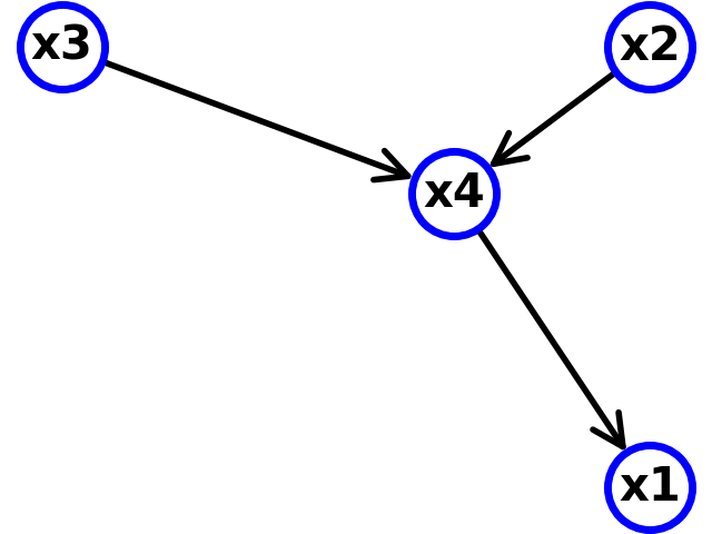
As the benchmarks are programs composed by a set of interdependent FP variables, the variables’ interactions represent a source of valuable information for learning the relationship between precision and error. This domain-level knowledge is encoded in the dependency graph of the benchmark, which specifies how the program variables are related. For instance, consider the expression ; this corresponds to four precision that need to be decided . The first three precision-variables , , and represent the precision of the actual variables of the expression, respectively , , and ; the last variable is a temporary variable introduced by FlexFloat to handle the (possibly) mismatching precision of the operands and (FlexFloat performs a cast from and to the intermediate precision ). Each variable is a node in the dependency graph, and the relations among variables are directed edges, as depicted in Fig. 1; an edge entering a node means that the precision of the source-variable is linked to the precision of the destination-variable.
4.3.1 Additional Features Extraction
As we have seen, the prior information on the benchmarks is encoded in directed graphs; for explanatory purposes, we will take as example the micro-benchmark represented by the graph in Fig. 1. Using the encoded knowledge, a set of additional features characterizing the precision configurations can be obtained. We consider only one type of relation, that is assignments (e.g. ). In this kind of expression, granting a larger number of bits to the value to be assigned would be pointless since the final precision of the expression is ultimately governed by the precision of the result variable . Configurations that respect this relationship have a higher probability to lead to smaller errors w.r.t. configurations that do not respect this constraint. In practice, configurations where are associated to smaller errors.
This information can be added to the training set as a collection of additional features. For each couple of variables involved in an assignment operation we compute the feature 33 3 If it means that the is not respected, hence a higher error is associated to the configuration, which is then added to the data set. Each feature corresponds to one of the logic binary constraints used to express the domain knowledge. For instance, if we consider again the example of Fig. 1 there are three additional features, one for each assignment expression (highlighted by the three arrows in the graph): , , . Thanks to these additional features an extended data set can be obtained. If we consider two possible configurations for the micro-benchmark in Fig. 1, and , the original data set would be composed by four features (one for each FP variable) plus the associate error (the target of the regression task). Instead, the extended data set contains seven features plus the error: and .
4.3.2 Graphical Convolutional Neural Networks
The transprecision learning task is a supervised regression problem whose prior information can be expressed through a graph, that is the dependency graph that links the variable in the benchmark. As mentioned in Section 3, GCNNs are well suited to deal with graph-structured problems. As our problem is slightly different from those considered in the literature, we did not adopted the standard approach but we rather exploited the main component of GCNNs, the graph convolution, implemented via Graph Convolutional Layers (GCL), and applied to the transprecision task. The GCNN has the following structure: first, from the dependency graph we compute the adjacency matrix; then the adjacency matrix and the input feature matrix are combined to form the input of a first GCL, which is then fed to a second one. Its output becomes the input for a fully connected dense layer with 128 neurons, followed by two other fully connected layers of decreasing dimension (respectively, 32 and 8). The final layer is, again, a dense layer with a single neuron, that is the network output.
4.3.3 Data Augmentation and Regularization
As mentioned in Sec. 4, the learning task is made more difficult by the presence of non-mononicity: situations where the normal precision-error relationship is not respected. They arise due to numerical instability, and their presence is magnified by the use of small data sets and a limited number of different input sets; with sufficiently large data sets they would be discarded as outliers. As mentioned before, the learning task addressed in this paper is a step towards an optimization model for precision tuning; with this scope in mind, it would be preferable to have a ML model that does not reproduce non-monotonicity events in its predictions. This is a domain knowledge about an undesirable propriety that should be corrected. The problem with non-monotonicity would be solved if we could have more training examples, but this is not easily attainable as we should run a benchmark to compute the error associated to a configuration. However, generating new configurations without computing the error is trivial; we can exploit this advantage in conjunction with an appropriate regularization scheme in order to impose monotonicity on the ML model predictions. This process is a form of data augmentation. Injecting the monotonicity constraint in the training process may allow to mitigate the noise and improve generalization, even with smaller training sets. We take into account such constraint at training time by exploiting ideas from Semantic Based Regularization [DGS17], an approach that advocates to the use of (differentiable) constraints as regularizers in the loss function. Let us write if configuration dominates , i.e. if every variable in has precision higher than or equal to ; let be the set of dominated-dominating pairs in our training set , . Then, we can formulate the following regularized loss function:
| (1) |
where is the error predictor being trained, and MSE is the mean squared error. Each regularization term is associated to a pair in and has non-zero value iff the error for the dominating pair is larger than for the dominated pair, i.e. if the monotonicity constraint is violated. New configurations in can be generated in order to get a much stable regularization factor without the need of a bigger train set
Is worth noticing that SBR is orthogonal to the use of additional features hence the two methods can be combined; we plan to explore the benefits of merging multiple methods in future works.
5 Experimental Evaluation
We selected 5 different purely data-driven models to obtain a baseline: I) a black-box optimization method (AutoSklearn); II) a NN composed of 4 dense layers with neurons each, that is, the number of variables in a benchmark multiplied by 10 (NN-1); III) a NN composed of 4 dense layers with neurons each (NN-2); IV) a NN composed of 10 dense layers with neurons each (NN-3); V) a NN composed of 20 dense layers with neurons each (NN-4). All NNs have a single-neuron output layer fully connected with the previous one. The black-box method used was drawn from the AutoML area, namely a framework called autosklearn [FKEea15] which uses Bayesian optimization for algorithm configuration and selection (e.g. finding the best set of hyperparameters for a given task). Our problem can be cast in the AutoML mold if we treat the variables precision as the algorithm configurations to be explored and the associated computation error as the target.
The code used to run the experiments was written in Python, using Keras and TensorFlow for the implementation of the neural networks. Autosklearn is distributed as a Python library and we used the version available online 44 4 https://automl.github.io/auto-sklearn/master/, with default parameters and letting the framework choose among all the implemented regression models. The GCNN model was created using the Spektral library 55 5 https://danielegrattarola.github.io/spektral/. All the results presented in this section were run on 20 different instances (different training and test sets) and we report the average values. Both input feature and targets were normalized. The code used to run the experiments is available at this online repository [REDACTED_FOR_BLIND_REVIEW].
To evaluate the impact of the additional features, the four different neural networks previously defined (NN-1, NN-2, NN-3, NN-4) were trained and tested both with and without the extended data set. At this stage we focus on the number of layers and their width and discarded other hyperparameters; their exploration will be the subject of future research works. In this paper, these are the values for the main hyperparameter used with all methods: number of epochs ; batch size ; as training algorithm we opted for Adam [KB14] with standard parameters; Mean Squared Error as loss function. The data augmentation and SBR approach is used on top of a neural network with the same number of layers and neurons as NN-1. The new configurations are injected in each batch during the training, with a fixed size of elements; the amount of data generated is specified by a ratio, which represents the percentage of samples introduced by the data augmentation.
5.1 Models Accuracy
We begin by evaluating the prediction accuracy of the proposed approaches. We measure the accuracy using the Mean Average Error (MAE). In Table1 we compare the results obtained using a training and test set size of, respectively, 5000 and 1000 examples; test and training set are randomly drawn from the samples generated through LHS. The first column of the table identifies the benchmark (the last row corresponds to the average over all of them); the second column contains the MAE obtained with the black-box approach, AutoSklearn; columns 3 and 4 report the MAE with the first NN (NN-1), respectively without and with the additional features; the three following couples of columns are the results with the other NNs (NN-2, NN-2, NN-3), again split between base and extended data set; the final two columns correspond respectively to MAE obtained with GCNN and with SBR. For this table, we consider the SBR approach with 75% of augmented examples – more details at Sec. 5.2.
| Benchmark | AutoSklearn | NN-1 | NN-2 | NN-3 | NN-4 | GCNN | SBR | ||||
|---|---|---|---|---|---|---|---|---|---|---|---|
| Base | Ext. | Base | Ext. | Base | Ext. | Base | Ext. | ||||
| FWT | 0.394 | 0.315 | 0.251 | 0.056 | 0.054 | 0.104 | 0.061 | 0.070 | 0.105 | 0.351 | 0.243 |
| saxpy | 0.003 | 0.000 | 0.000 | 0.000 | 0.000 | 0.000 | 0.000 | 0.000 | 0.000 | 0.000 | 0.001 |
| convolution | 0.020 | 0.005 | 0.005 | 0.002 | 0.002 | 0.003 | 0.003 | 0.003 | 0.003 | 0.004 | 0.006 |
| correlation | 0.397 | 0.139 | 0.120 | 0.091 | 0.092 | 0.111 | 0.098 | 0.114 | 0.102 | 0.262 | 0.139 |
| dwt | 0.422 | 0.057 | 0.034 | 0.011 | 0.012 | 0.029 | 0.020 | 0.031 | 0.022 | 0.072 | 0.068 |
| BlackScholes | 0.411 | 0.238 | 0.047 | 0.184 | 0.035 | 0.239 | 0.038 | 0.297 | 0.172 | 0.307 | 0.220 |
| Average | 0.274 | 0.126 | 0.076 | 0.057 | 0.033 | 0.081 | 0.037 | 0.086 | 0.067 | 0.166 | 0.113 |
The black-box model AutoSklearn has clearly the worst performance, which is not entirely surprising given the complexity of the learning task. The first unexpected and disappointing result is the poor performance of the GCNN, that is outperformed by all other approaches in almost all benchmarks. We remark that this was a novel application of GCNN and this preliminary analysis merely suggests that a more careful exploration is needed. Changing the network type can produce good results: using a wider NN (from NN-1 to NN-2) greatly reduces the MAE, while deeper NNs provide smaller improvements (e.g. NN-3 and NN-4). Very interestingly, a major MAE reduction is obtained by using the additional features (column Ext.): for all NN types and over all benchmarks, the approach using the extended data greatly outperforms the baseline, with an average improvement of 39.7% (considering all four NN types). The results obtained with data agumentation and SBR show that this method performs better than AutoSklearn and the simplest NN without the additional features (NN-1), but it has a higher MAE compared to all the approaches with the extended data set. This is not an issue as SBR benefits were not expected in terms of prediction accuracy but rather on the enforcing of the monotonicity (see Sec. 5.2).
We are also interested in measuring the results with smaller training sets, again using MAE as metric; we keep the test set size fixed at 1000 elements. Table 2 reports the experimental results; it has the same structure of Tab. 1. As expected, the prediction accuracy decreases with the training set size, but the benefits brought by the domain knowledge remain – over all training set size, the improvement brought by the engineered features is 38.7%.
| Train Set Size | AutoSklearn | NN-1 | NN-2 | NN-3 | NN-4 | GCNN | SBR | ||||
|---|---|---|---|---|---|---|---|---|---|---|---|
| Base | Ext. | Base | Ext. | Base | Ext. | Base | Ext. | ||||
| 500 | 0.288 | 0.196 | 0.131 | 0.100 | 0.064 | 0.140 | 0.078 | 0.144 | 0.134 | 0.316 | 0.190 |
| 1000 | 0.285 | 0.178 | 0.107 | 0.087 | 0.048 | 0.108 | 0.056 | 0.142 | 0.117 | 0.256 | 0.181 |
| 2000 | 0.278 | 0.155 | 0.085 | 0.077 | 0.041 | 0.094 | 0.047 | 0.119 | 0.060 | 0.210 | 0.162 |
| 5000 | 0.274 | 0.126 | 0.076 | 0.057 | 0.033 | 0.081 | 0.037 | 0.086 | 0.067 | 0.166 | 0.133 |
5.2 Semantic Based Regularization Impact
This section provides additional details on the experiments on data augmentation and SBR. The model was tested on the previous benchmarks and different ratios of data injected, i.e. 25% and 75%. In order to have a more precise evaluation of the approach, we relied on another metric beside MAE, that is the number of violated monotonicity constraints – the goal of this approach is to reduce their number. We underline that not every benchmark had monotonicity issues (as they are outliers), and in these cases the regularization factor is of no use and might keep the model from a good approximation. For this reason, Table 3 and Table 4, report just the values from significant benchmarks (i.e. benchmarks that exhibit the most marked non-monotonic behavior), these are convolution and correlation. The third column reports the result obtained with NN-1 without the additional features. Columns 4-6 correspond to the results obtained with data augmentation and SBR, with different percentages of injected data (0%, 25%, 75%)
| Benchmark | Size | NN-1 | SBR | SBR 25% | SBR 75% |
|---|---|---|---|---|---|
| MAE | MAE | MAE | MAE | ||
| convolution | 0.012 | 0.019 | 0.013 | 0.011 | |
| 0.005 | 0.006 | 0.006 | 0.006 | ||
| correlation | 0.263 | 0.265 | 0.263 | 0.262 | |
| 0.139 | 0.059 | 0.059 | 0.139 |
| Benchmark | Size | NN-1 | SBR | SBR 25% | SBR 75% |
|---|---|---|---|---|---|
| #Viol. | #Viol. | #Viol. | #Viol. | ||
| convolution | 168 | 156 | 171 | 126 | |
| 0 | 13 | 12 | 6 | ||
| correlation | 111 | 120 | 116 | 98 | |
| 91 | 59 | 71 | 92 |
With larger training sets, the benefits of data augmentation and SBR are marginal: the additional constraint on the loss function is not very useful, given the abundance of training samples allowing for better generalization. Similarly, larger training sets lead to a natural decrease in the number of monotonicity constraints violated (as their proportion in the training set diminishes). Nevertheless, the more interesting results can be observed when fewer data points are available, since the models show a decrease in the number of violated constraints opposed to the network without regularization. Furthermore, the networks performed better with higher ratios of data injected, i.e. 18%, on average. Finally, the MAE seems to have values compatible to the results obtained with NN-1, a good result since prediction accuracy was not SBR’s scope. These results encourage the idea of a hybrid model merging data augmentation plus SBR and additional features (both approaches enabled by the injection of domain knowledge), as future development of this work.
6 Conclusion & Future Works
In this paper we present a strategy for injecting domain knowledge in a ML model. As a case of study, we considered a learning task from the transprecision computing field, namely predicting the computation error associated to the precision used for handling a set of FP variables composing a benchmark. This is a difficult regression problem, hard to be addressed with pure data-driven ML methods; we have shown how critical improvements can be reached by injecting domain knowledge in the ML models.
We introduced three knowledge-injection approaches and applied them on top of NNs with varying structures: feature engineering, a GCNN, and a data augmentation scheme enabled by SBR. The GCNN approach did not improve the accuracy of the ML model w.r.t. the baseline and it should be explored more in detail. Conversely, the creation of extended data set was revealed to be extremely useful, leading to remarkable reduction in prediction error (39.7% on average and up to 47.5% in the best case). Data augmentation plus SBR showed its potential with training sets of limited size, in terms of reduced number of violated monotonicity constraints while preserving the ML models’ prediction accuracy.
In future works we plan to integrate the learners in an optimization model for solving the FP tuning precision problem. In this regard we will explore active learning strategies and we expect SBR to have good result, especially when combined with the additional features (the methods are orthogonal). Moreover, we will perform experiments with other domain knowledge injection approaches, for instance by building data sets in accordance with the prior information and by exploiting the knowledge to guide the training of the NN by constraining its output.
Acknowledgments
This work has been partially supported by European H2020 FET project OPRECOMP (g.a. 732631).
References
- [CW19] Christopher M Childs and Newell R Washburn. Embedding domain knowledge for machine learning of complex material systems. MRS Communications, 9(3):806–820, 2019.
- [DBV16] Michaël Defferrard, Xavier Bresson, and Pierre Vandergheynst. Convolutional neural networks on graphs with fast localized spectral filtering. In Advances in neural information processing systems, pages 3844–3852, 2016.
- [DGS17] Michelangelo Diligenti, Marco Gori, and Claudio Sacca. Semantic-based regularization for learning and inference. Artificial Intelligence, 244:143–165, 2017.
- [DK17] Eva Darulova and Viktor Kuncak. Towards a compiler for reals. ACM Trans. Program. Lang. Syst., 39(2):8:1–8:28, March 2017.
- [FBDC+18] Marc Fischer, Mislav Balunovic, Dana Drachsler-Cohen, Timon Gehr, Ce Zhang, and Martin Vechev. Dl2: Training and querying neural networks with logic. 2018.
- [FKEea15] Matthias Feurer, Aaron Klein, Katharina Eggensperger, and et al. Efficient and robust automated machine learning. In Advances in neural information processing systems, pages 2962–2970, 2015.
- [HMWA17] Nhut-Minh Ho, Elavarasi Manogaran, Weng-Fai Wong, and Asha Anoosheh. Efficient floating point precision tuning for approximate computing. In Design Automation Conference (ASP-DAC), 2017 22nd Asia and South Pacific, pages 63–68. IEEE, 2017.
- [KB14] Diederik P Kingma and Jimmy Ba. Adam: A method for stochastic optimization. arXiv preprint arXiv:1412.6980, 2014.
- [KST18] Udayan Khurana, Horst Samulowitz, and Deepak Turaga. Feature engineering for predictive modeling using reinforcement learning. In Thirty-Second AAAI Conference on Artificial Intelligence, 2018.
- [KW17] Thomas N. Kipf and Max Welling. Semi-Supervised Classification with Graph Convolutional Networks. In Proceedings of the 5th International Conference on Learning Representations, ICLR ’17, 2017.
- [LS19] Tao Li and Vivek Srikumar. Augmenting neural networks with first-order logic. arXiv preprint arXiv:1906.06298, 2019.
- [MIM+18] Nikhil Muralidhar, Mohammad Raihanul Islam, Manish Marwah, Anuj Karpatne, and Naren Ramakrishnan. Incorporating prior domain knowledge into deep neural networks. In 2018 IEEE International Conference on Big Data (Big Data), pages 36–45. IEEE, 2018.
- [MLG14] Violeta Mirchevska, Mitja Luštrek, and Matjaž Gams. Combining domain knowledge and machine learning for robust fall detection. Expert Systems, 31(2):163–175, 2014.
- [MSea18] A Cristiano I Malossi, Michael Schaffner, and et al. The transprecision computing paradigm: Concept, design, and applications. In Design, Automation & Test in Europe Conference & Exhibition (DATE), 2018, pages 1105–1110. IEEE, 2018.
- [MTDM17] Mariano Moscato, Laura Titolo, Aaron Dutle, and César A Munoz. Automatic estimation of verified floating-point round-off errors via static analysis. In International Conference on Computer Safety, Reliability, and Security, pages 213–229. Springer, 2017.
- [MYG19] Rebecca Miao, Zhenyi Yang, and Valeriy Gavrishchaka. Leveraging domain-expert knowledge, boosting and deep learning for identification of rare and complex states. In Journal of Physics: Conference Series, volume 1207, page 012016. IOP Publishing, 2019.
- [NVG19] Liudmyla Nechepurenko, Viktor Voss, and Vyacheslav Gritsenko. Comparing knowledge-based reinforcement learning to neural networks in a strategy game. arXiv preprint arXiv:1901.04626, 2019.
- [opr] Oprecomp - open transprecision computing. http://oprecomp.eu/. Online; accessed 15 May 2019.
- [Ste87] Michael Stein. Large sample properties of simulations using latin hypercube sampling. Technometrics, 29(2):143–151, 1987.
- [TMea18] Giuseppe Tagliavini, Stefan Mach, and et al. A transprecision floating-point platform for ultra-low power computing. In Design, Automation & Test in Europe Conference & Exhibition (DATE), 2018, pages 1051–1056. IEEE, 2018.
- [XZF+17] Jingyi Xu, Zilu Zhang, Tal Friedman, Yitao Liang, and Guy Van den Broeck. A semantic loss function for deep learning with symbolic knowledge. arXiv preprint arXiv:1711.11157, 2017.
- [YSJ10] Ting Yu, Simeon Simoff, and Tony Jan. Vqsvm: A case study for incorporating prior domain knowledge into inductive machine learning. Neurocomputing, 73(13-15):2614–2623, 2010.
- [ZC18] Alice Zheng and Amanda Casari. Feature engineering for machine learning: principles and techniques for data scientists. ” O’Reilly Media, Inc.”, 2018.
- [ZTXM19] Si Zhang, Hanghang Tong, Jiejun Xu, and Ross Maciejewski. Graph convolutional networks: a comprehensive review. Computational Social Networks, 6(1):11, 2019.