Fermionic state discrimination by local operations and classical communication

In quantum theory, we may perfectly discriminate between any two orthogonal states $\ket{\psi}$, $\ket{\phi}$ of a bipartite system ${\rm A}{\rm B}$ through LOCC measurements Walgate et al. 2000. We remind that the most general case of a quantum measurement is represented by a POVM (POVM), i.e., a collection of effects (positive operators $0\leq S\leq I$) that sum to the identity operator $I$. A necessary condition for a POVM to represent a LOCC measurement is to be separable ( SEP (SEP)). The effect $S$ is separable if there exists some operators $0\leq A_{i},B_{i}\leq I$ such that $S=\sum_{i}A_{i}\otimes B_{i}$, and a povm represents a separable measurement if it is exclusively made of separable effects. Moreover, we recall that LOCC POVM are a proper subset of SEP POVM Bennett et al. 1999. In the following we will use the acronyms LOCC and SEP to denote the corresponding subsets of POVM.

We now give a sketchy summary of the result of Ref. Walgate et al. 2000. Every pair of orthogonal bipartite pure states can then be written as

where $\{\ket{i}_{\rm A}\}$ is a suitable orthonormal basis in the Hilbert space of Alice’s system, and $\{\ket{\eta_{i}}_{\rm B}\}$ and $\{\ket{\nu_{i}}_{\rm B}\}$ are sets of vectors in Bob’s Hilbert space that are pairwise orthogonal, i.e., $\braket{\eta_{i}|\nu_{i}}=0$. Alice has to measure her system in the given basis and send the outcome to Bob, who in turn manages to locally discriminate between two orthogonal states, thus inferring the correct result. Existence of the decomposition in Eq. (1) was shown in Ref. Walgate et al. 2000.

We follow here a strategy similar to the quantum one in order to distinguish between two pure orthogonal states $\ket{\psi}$, $\ket{\phi}$ of a bipartite Fermionic system. First of all, we notice that whenever the two preparations have different parity, e.g., $\ket{\psi}\in\mathcal{F}_{e}({\rm A}{\rm B})$ and $\ket{\phi}\in\mathcal{F}_{o}({\rm A}{\rm B})$, it is always possible to perfectly discriminate between the two just through local measurements. Indeed, Alice and Bob have to locally measure the parity of their subsystems and if their outcomes match, then the provided state was even, otherwise it was the odd one. The nontrivial case then is that of two pure states with the same parity. Since the even and odd sector are equivalent under LOCC, it is not restrictive to focus on even vectors only. We introduce the following convenient notation for the even vectors $\ket{\psi},\ket{\phi}\in\mathcal{F}_{e}({\rm A}{\rm B})$,

and recalling the decomposition in Ref. Walgate et al. 2000, we decompose $\ket{\psi_{E}}=\sum_{i=1}^{n}\ket{e_{i}}_{\rm A}\ket{\eta^{e}_{i}}_{\rm B}$, $\ket{\psi_{O}}=\sum_{i=1}^{n}\ket{o_{i}}_{\rm A}\ket{\eta^{o}_{i}}_{\rm B}$, $\ket{\phi_{E}}=\sum_{i=1}^{n}\ket{e_{i}}_{\rm A}\ket{\nu^{e}_{i}}_{\rm B}$, $\ket{\phi_{O}}=\sum_{i=1}^{n}\ket{o_{i}}_{\rm A}\ket{\nu^{o}_{i}}_{\rm B}$, where $\{\ket{e_{i}}\}$, $\{\ket{o_{i}}\}$ are Alice orthonormal bases of even and odd vectors, respectively, while $\{\ket{\eta^{x}_{i}}_{\rm B}\}$, and $\{\ket{\nu^{x}_{i}}_{\rm B}\}$, for $x=e,o$ are Bob vectors resulting from the decomposition. In general, the latter are not normalized and $\braket{\eta_{i}^{x}|\nu_{i}^{x}}_{\rm B}\neq 0$. We may indicate with the capitalized letters $E$ or $O$ those entities pertaining to the $E$ and $O$ spaces of $\mathcal{F}_{e}({\rm A}{\rm B})$, i.e., those subspaces where the parities of Alice’s and Bob’s subsystems are both even or odd, respectively. E.g., the $E$ part of vector $\ket{\psi}$ is defined as $\ket{\psi_{E}}=\sum_{i=1}^{n}\ket{e_{i}}_{\rm A}\ket{\eta^{e}_{i}}_{\rm B}$, whereas the $O$ part is $\ket{\psi_{O}}=\sum_{i=1}^{n}\ket{o_{i}}_{\rm A}\ket{\nu^{o}_{i}}_{\rm B}$. The orthogonality condition $\braket{\psi|\phi}=0$ generally reads

Let us consider as the first case the scenario where the two preparations have only one component. Then they have components either in complementary subspaces, e.g., $\ket{\psi}=\ket{\psi_{E}}$ and $\ket{\phi}=\ket{\phi_{O}}$, and it is trivially possible to discriminate via LOCC by measuring the local parities, or in the same subspace, e.g., $\ket{\psi}=\ket{\psi_{E}}$ and $\ket{\phi}=\ket{\phi_{E}}$. In the latter case the protocol reduces to the quantum one. Indeed, Alice selects the right basis $\{\ket{e_{i}}\}$ and lets Bob perfectly discriminate between $\ket{\eta^{e}_{i}}$ and $\ket{\nu^{e}_{i}}$, which are now orthogonal thanks to the result of Ref. Walgate et al. 2000. Moreover, as proved in Ref. D’Ariano et al. 2014b, product POVM in the Jordan-Wigner representation correspond to LOCC Fermionic POVM.

As the second case, we consider the situation where only one component out of the four $\ket{\psi_{E}}$, $\ket{\psi_{O}}$, $\ket{\phi_{E}}$, $\ket{\phi_{O}}$ is null. Perfect discrimination is implementable through LOCC in this case as well. Let us take for instance the vectors $\ket{\psi}=\ket{\psi_{E}}+\ket{\psi_{O}}$, and $\ket{\phi}=\ket{\phi_{O}}$; Alice and Bob firstly measure the parity of their subsystem and if the outcome is even, they know for sure that the system has been prepared in the state $\ket{\psi}$. Otherwise, the state after the measurement is either $\ket{\psi_{O}}/\|{\psi_{O}}\|$ or $\ket{\phi_{O}}$, and the above strategy for the first case applies.

In the most general case all four components are non-null. If the two $E$ and $O$ parts are orthogonal—that is when $\braket{\psi_{E}|\phi_{E}}=\braket{\psi_{O}|\phi_{O}}=0$—Alice and Bob can measure locally the parity of their systems, thus obtaining the post-measurement states $\ket{\psi^{\prime}}=\ket{\psi_{E}}/\|{\psi_{E}}\|$ and $\ket{\phi^{\prime}}=\ket{\phi_{E}}/\|{\phi_{E}}\|$ if the outcomes are both even, $\ket{\psi^{\prime}}=\ket{\psi_{O}}/\|{\psi_{O}}\|$ and $\ket{\phi^{\prime}}=\ket{\phi_{O}}/\|{\phi_{O}}\|$ if the outcomes are both odd. Consequently they reduced to the first case.

There is one situation left fulfilling condition (3), i.e., when $\braket{\psi_{E}|\phi_{E}}\neq 0$ and $\braket{\psi_{O}|\phi_{O}}\neq 0$. This case exhibits the main difference with respect to quantum theory. Consider for instance the states $1/\sqrt{2}(\ket{00}_{\rm A}\ket{00}_{\rm B}\pm\ket{01}_{\rm A}\ket{01}_{\rm B})$. In this case, the decompositions in Eq. (1) involves bases $\{\ket{\eta_{i}}_{\rm B}\}$ and $\{\ket{\nu_{i}}_{\rm B}\}$ where superpositions forbidden by the Fermionic superselection rule appear. Indeed, one has $i=\pm$ and

The last case can thus not be treated by straightforwardly applying the quantum strategy of Ref. Walgate et al. 2000. The following theorem summarizes what we discussed so far, and shows that it is not possible to perfectly discriminate two states with $\braket{\psi_{E}|\phi_{E}}\neq 0$ and $\braket{\psi_{O}|\phi_{O}}\neq 0$ through POVM in SEP, thus neither by means of LOCC.

We now show that one can overcome the limits of Theorem 1 by providing the two parties with an ancillary system prepared in a suitable pure entangled state $\ket{\omega}$. Let us take

and consider the task of discriminating the new vectors $\ket{\psi^{\prime}}\coloneqq\ket{\psi}\otimes\ket{\omega}$ and $\ket{\phi^{\prime}}\coloneqq\ket{\phi}\otimes\ket{\omega}$. In particular, we will see that only a maximally entangled ancillary state—i.e., with $\mathinner{\!\left\lvert a\right\rvert}^{2}=\mathinner{\!\left\lvert b\right\rvert}^{2}=1/2$—enables perfect discrimination between every two pure Fermionic states, regardless of condition (4).

If the orthogonality condition $\braket{\psi|\phi}=0$ is relaxed, the two states are clearly not perfectly discriminable. Hence, one looks for the protocol which minimizes the error probability—i.e., the probability of wrong detection. For this purpose, it is necessary to introduce our prior probabilities for the two states, given by the distribution $\{p,q\}$. In this case, the error probability reads

where $\{\Pi_{\psi},\Pi_{\phi}\}$ is the binary POVM describing the discrimination protocol. We remind that by definition the POVM satisfies $\Pi_{\psi},\Pi_{\phi}\geq 0$ and $\Pi_{\psi}+\Pi_{\phi}=I$. In the quantum case, the optimal discrimination strategy corresponds to the POVM $\{\ket{+}\bra{+},\ket{-}\bra{-}\}$ diagonalizing the operator

where $\lambda_{+}>0$, $\lambda_{-}<0$ are the eigenvalues of $\Delta$, and $\braket{+|-}=0$ (see Refs. Helstrom 1969; Helstrom 1976). The corresponding error probability is Helstrom 1976

In Ref. Virmani et al. 2001, the authors observe that optimal discrimination through LOCC of $\ket{\psi}$ and $\ket{\phi}$ with prior probabilities $p$ and $q$, respectively, is equivalent to perfect LOCC discrimination between $\ket{+}$ and $\ket{-}$ (see also Ref. Helstrom 1976), thus reducing the optimal case to an instance of perfect discrimination. While the latter is always possible in quantum theory, we know from Theorem 1 that in Fermionic theory this is true only if the eigenvectors satisfy

Otherwise, by Theorem 2 perfect LOCC discrimination requires a maximally entangled ancilla. As for the perfect discrimination case, also the conditions for optimal LOCC discrimination in Fermionic theory differ from the quantum ones only when the $E$ and $O$ components of $\ket{+}$ and $\ket{-}$ are all non-zero, and $\braket{+_{E}|-_{E}},\braket{+_{O}|-_{O}}\neq 0$. For the latter case, we now prove a necessary and sufficient condition for achievability of optimal discrimination with LOCC that does not require diagonalization of $\Delta$.

We may wonder what happens when condition (12) is not satisfied. As we show in the next theorem, the best discrimination strategy through SEP corresponds to measuring in the basis of eigenvectors of $\Delta_{E}$ and $\Delta_{O}$, defined as the restriction of the operator $\Delta$ onto the $E$ and $O$ subspaces, respectively. Such a strategy is LOCC.

The above result allows us to treat the case where we are restricted only to local measurements and Eq. (12) does not hold for the preparations $\rho$, $\sigma$. Once we are given the pure states $\ket{\psi}$ and $\ket{\phi}$, the condition for optimal LOCC discrimination of Eq. (12) is fulfilled either for the vectors laying in the $E$ or $O$ space, i.e., $[\ket{\psi}\bra{\psi},P_{E}]=[\ket{\phi}\bra{\phi},P_{E}]=0$, or if the probability $p$ satisfies

Condition (16) can be satisfied by a unique value of the prior probability $p$, unless $[\ket{\psi}\bra{\psi},P_{E}]=[\ket{\phi}\bra{\phi},P_{E}]=0$. However, we now show that optimal LOCC discrimination can achieve the performances of unconstrained protocols, provided that two ancillary Fermionic systems are used in a maximally entangled state. As discussed above, indeed, the problem of optimal discrimination between two pure states reduces to that of the orthogonal vectors $\ket{+},\ket{-}$ in Eq. (9). Considering Theorem 2, we know that orthogonal states can be perfectly discriminated via LOCC provided a maximally entangled ancillary system is available. These two observations immediately lead to our last result.

Equation (16) introduces a strict condition on the prior probability of the preparations, which are always subject to noise. We show hereafter that if we introduce a small perturbation $\epsilon$ on the preparation probabilities of pair of states satisfying Eq. (12), the discrimination error probability increases at most linearly in $\epsilon$ with respect to the appropriate optimal LOCC protocol. Thus, we map $p\mapsto p+\epsilon$ and attain

where $[\Delta^{0},P_{E}]=0$. At this stage, we estimate the error difference between the optimal povm $\mathbb{P}^{0}\coloneqq\{\Pi_{\psi},\Pi_{\phi}\}$ for $\epsilon=0$, which is LOCC thanks to Theorem 3, and the LOCC-optimal povm for the perturbed case $\Delta^{\epsilon}$. The error increases as $\delta\mathcal{P}_{\text{err}}\coloneqq\mathcal{P}_{\text{err}}(\mathbb{P}^{0}|\Delta^{\epsilon})-\mathcal{P}_{\text{err}}^{\mathsf{LOCC}}(\Delta^{\epsilon})\geq 0$ where $\mathcal{P}_{\text{err}}(\mathbb{P}^{0}|\Delta^{\epsilon})={\rm Tr}[(p+\epsilon)\ket{\psi}\bra{\psi}\Pi_{\phi}+(q-\epsilon)\ket{\phi}\bra{\phi}\Pi_{\psi}]$ and $\mathcal{P}_{\text{err}}^{\mathsf{LOCC}}(\Delta^{\epsilon})=\frac{1}{2}(1-\|{\Delta_{E}^{\epsilon}+\Delta_{O}^{\epsilon}}\|_{1})$ as in Eq. (15). Accordingly manipulating the expression for $\delta\mathcal{P}_{\text{err}}$ one obtains

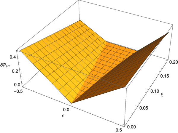
where $k,g\geq 0$ are suitable constants depending only on $\ket{\psi}$, $\ket{\phi}$. The former inequality is as tight as possible: let us take indeed the states $\ket{\psi}=1/\sqrt{2}\ket{00}+1/\sqrt{2}\ket{11}$ and $\ket{\phi}=\alpha\ket{00}+\sqrt{1-\alpha^{2}}\ket{11}$, where $\alpha\coloneqq(1/\sqrt{2}+\xi)$, and $\xi$ belongs to a neighborhood of zero. In such a case, we have numerically assessed that the error difference $\delta\mathcal{P}_{\text{err}}$ exhibits a corner in $\epsilon=0$ as $\xi\to 0$ (more details can be found in the Supplemental Material).

We also investigate the performance of the optimal LOCC protocol for $\epsilon\neq 0$ in the neighborhood of a prior probability $p$ satisfying condition (16), by comparing its efficiency to that of the optimal unconstrained (i.e., entanglement-assisted LOCC) povm. Thus we estimate $\delta\mathcal{P}_{\text{err}}^{\prime}\coloneqq\mathcal{P}_{\text{err}}^{\mathsf{LOCC}}(\Delta^{\epsilon})-\mathcal{P}_{\text{err}}(\Delta^{\epsilon})\geq 0$ by means of Eqs. (10) and (15), obtaining

for a suitable $\kappa\geq 0$, thanks to the triangle inequality.

We remark that, in the case of a mismatch in the assessment of the prior probability $p$, also for unconstrained optimal discrimination—coinciding with ancilla-assisted LOCC—one has the same bound as in Eq. (17), with possibly different constants $k$ and $g$. This feature, however, must not be considered as an artefact of Fermionic theory. Indeed, the technique used to derive the bound in Eq. (17) is very general and leads to the same behavior in the quantum case as well.

As in the quantum case, discrimination with separable and LOCC POVM in the Fermionic case achieve the same performances. Unlike in quantum theory, on the other hand, in Fermionic theory ideal state discrimination through LOCC is subject to non-trivial conditions. In this Letter, we derived the conditions under which LOCC discrimination achieves the ideal performances of unconstrained discrimination protocols. However, in the Fermionic case, ancilla-assisted LOCC protocols achieve ideal discrimination. One has to remark, though, that this is the case only for maximally entangled ancillary states. The former statement unequivocally determines the amount of entanglement required for such a task. We finally studied the behavior of optimal protocols—which depend on prior probabilities of the states to be discriminated—if the prior conditions are subject to perturbation. A remarkable instability is observed, corresponding to a corner point in the curve representing the error probability excess due to non-optimized POVM. We stress that the latter phenomenon is not exclusive of Fermionic theory, as it occurs also in the quantum case.