Temporal Spike Sequence Learning via Backpropagation for Deep Spiking Neural Networks
Abstract
Spiking neural networks (SNNs) are well suited for spatio-temporal learning and implementations on energy-efficient event-driven neuromorphic processors. However, existing SNN error backpropagation (BP) methods lack proper handling of spiking discontinuities and suffer from low performance compared with the BP methods for traditional artificial neural networks. In addition, a large number of time steps are typically required to achieve decent performance, leading to high latency and rendering spike based computation unscalable to deep architectures. We present a novel Temporal Spike Sequence Learning Backpropagation (TSSL-BP) method for training deep SNNs, which breaks down error backpropagation across two types of inter-neuron and intra-neuron dependencies and leads to improved temporal learning precision. It captures inter-neuron dependencies through presynaptic firing times by considering the all-or-none characteristics of firing activities, and captures intra-neuron dependencies by handling the internal evolution of each neuronal state in time. TSSL-BP efficiently trains deep SNNs within a much shortened temporal window of a few steps while improving the accuracy for various image classification datasets including CIFAR10.
1 Introduction
Spiking neural networks (SNNs), a brain-inspired computational model, have gathered significant interests [9]. The spike-based operational principles of SNNs not only allow information coding based on efficient temporal codes and give rise to promising spatiotemporal computing power but also render energy-efficient VLSI neuromorphic chips such as IBM’s TrueNorth [1] and Intel’s Loihi [6]. Despite the recent progress in SNNs and neuromorphic processor designs, fully leveraging the theoretical computing advantages of SNNs over traditional artificial neural networks (ANNs) [17] to achieve competitive performance in wide ranges of challenging real-world tasks remains difficult.
Inspired by the success of error backpropagation (BP) and its variants in training conventional deep neural networks (DNNs), various SNNs BP methods have emerged, aiming at attaining the same level of performance [4, 16, 24, 13, 21, 28, 11, 2, 3, 29]. Although many appealing results are achieved by these methods, developing SNNs BP training methods that are on a par with the mature BP tools widely available for training ANNs today is a nontrivial problem [22].
Training of SNNs via BP are challenged by two fundamental issues. First, from an algorithmic perspective, the complex neural dynamics in both spatial and temporal domains make the BP process obscure. Moreover, the errors are hard to be precisely backpropagated due to the non-differentiability of discrete spike events. Second, a large number of time steps are typically required for emulating SNNs in time to achieve decent performance, leading to high latency and rendering spike based computation unscalable to deep architectures. It is desirable to demonstrate the success of BP in training deeper SNNs achieving satisfactory performances on more challenging datasets. We propose a new SNNs BP method, called temporal spike sequence learning via BP (TSSL-BP), to learn any target output temporal spiking sequences. TSSL-BP acts as a universal training method for any employed spike codes (rate, temporal, and combinations thereof). To tackle the above difficulties, TSSL-BP breaks down error backpropagation across two types of inter-neuron and intra-neuron dependencies, leading to improved temporal learning precision. It captures the inter-neuron dependencies within an SNN by considering the all-or-none characteristics of firing activities through presynaptic firing times; it considers the internal evolution of each neuronal state through time, capturing how the intra-neuron dependencies between different firing times of the same presynaptic neuron impact its postsynaptic neuron. The efficacy and precision of TSSL-BP allows it to successfully train SNNs over a very short temporal window, e.g. over 5-10 time steps, enabling ultra-low latency spike computation. As shown in Section 4, TSSL-BP signficantly improves accuracy and runtime efficiency of BP training on several well-known image datasets of MNIST [15], NMNIST [19], FashionMNIST [26], and CIFAR10 [14]. Specifically, it achieves up to accuracy improvement over the previously reported SNN work on CIFAR10, a challenging dataset for all prior SNNs BP methods.
2 Background
2.1 Existing Backpropagation methods for SNNs
One of the earliest SNNs BP methods is the well-known SpikeProp algorithm [4]. However, SpikeProp and its variants [5, 10, 27] are still limited to single spike per output neuron without demonstrating competitive performance on real-world tasks. In addition, [7, 8, 12, 20] train ANNs and then approximately convert them to SNNs. Nevertheless, such conversion leads to approximation errors and cannot exploit SNNs’ temporal learning capability.
Recently, training SNNs with BP under a firing rate (or activity level) coded loss function has been shown to deliver competitive performances [16, 24, 21, 13, 28, 11, 2, 29]. Among them, [16] does not consider the temporal correlations of neural activities and treats spiking times as noise to allow error gradient computation. [21, 24, 28, 2] capture the temporal effects by performing backpropagation through time (BPTT) [23]. However, they get around the non-differentiability of spike events by approximating the spiking process using the surrogate gradient method [18]. These approximations lead to inconsistency between the computed gradient and target loss, and thus degrade training performance. [11] presents a BP method for recurrent SNNs based on a novel combination of a gate function and threshold-triggered synaptic model that are introduced to handle non-differentiability of spikes. In this work, depolarization of membrane potential within a narrow active zone below the firing threshold also induces graded postsynaptic current. [13, 29] present spike-train level BP methods by capturing the effects of spiking neurons aggregated at the spike train level. However, the length of spike trains over which BP is applied need to be long enough, leading to long inference latency and high training cost.
[25] can train SNNs over a relatively small number of time steps by adding optimization techniques such as neuron normalization and population decoding. Since its core lies at the method of [24], it still approximates the all-or-none firing characteristics of spiking neurons by a continuous activation function, causing the same problems introduced before.
In this work, we propose the TSSL-BP method as a universal training method for any employed spike codes. It can not only precisely capture the temporal dependencies but also allow ultra-low latency inference and training over only five time steps while achieving excellent accuracies.
2.2 Spiking Neuron Model
SNNs employ more biologically plausible spiking neuron models than ANNs. In this work, we adopt the leaky integrate-and-fire (LIF) neuron model and synaptic model [9].
Consider the input spike train from pre-synaptic neuron to neuron : , where denotes a particular firing time of presynaptic neuron . The incoming spikes are converted into an (unweighted) postsynaptic current (PSC) through a synaptic model. The neuronal membrane voltage at time for neuron is given by
| (1) |
where and are the effective leaky resistance and time constant of the membrane, is the synaptic weight from pre-synaptic neuron to neuron , is the (unweighted) postsynaptic potential (PSC) induced by the spikes from pre-synaptic neuron , and denotes the reset function.
The PSC and the reset function can be written as
| (2) |
where and are the spike response and reset kernel, respectively. In this work, we adopt a first order synaptic model as the spike response kernel which is expressed as:
| (3) |
where is the synaptic time constant.
The reset kernel reduces the membrane potential by a certain amount , where is equal to the firing threshold right after the neuron fires. Considering the discrete time steps simulation, we use the fixed-step first-order Euler method to discretize (1) to
| (4) |
The ratio of R and is absorbed into the synaptic weight. The reset function represents the firing-and-resetting mechanism of the neuron model. Moreover, the firing output of the neuron is expressed as
| (5) |
where is the firing threshold and is the Heaviside step function.
3 Methods
3.1 Forward Pass
Without loss of generality, we consider performing BP across two adjacent layers and with and neurons, respectively, in a fully-connected feedforward SNNs as shown in Figure 1. The procedure can be also applied to convolutional and pooling layers. Denote the presynaptic weights by , where is a column vector of weights from all the neurons in layer to the neuron of layer . In addition, we also denote PSCs from neurons in layer by , spike trains output of the layer by , membrane potentials and the corresponding output spike trains of the layer neurons respectively by and , where variables associated with neurons in the layer have as the superscript.
The forward propagation between the two layers is described as
| (6) | ||||
In the forward pass, the spike trains of the layer generate the (unweighted) PSCs according to the synaptic model. Then, are multiplied the synaptic weights and passed onto the neurons of layer . The integrated PSCs alter the membrane potentials and trigger the output spikes of the layer neurons when the membrane potentials exceed the threshold.
3.2 The Loss Function
The goal of the proposed TSSL-BP method is to train a given SNN in such a way that each output neuron learns to produce a desired firing sequence arbitrarily specified by the user according to the input class label. Denote the desired and the actual spike trains in the output layer by and where is the number of the considered time steps, and the desired and actual firing events for all output neurons at time , respectively.
The loss function can be defined using any suitable distance function measuring the difference between and . In this work, the loss function is defined by the total square error summed over each output neuron at each time step:
| (7) |
where is the error at time and a kernel function which measures the so-called Van Rossum distance between the actual spike train and desired spike train.
3.3 Temporal Spike Sequence Learning via Backpropagation (TSSL-BP) Method
From the loss function (7), we define the error at each time step. is based on the output layer firing spikes at which further depend on all neuron states , . Below we consider these temporal dependencies and derive the main steps of the proposed TSSL-BP method. Full details of the derivation are provided in Section 1 of the Supplementary Material.
Using (7) and the chain rule, we obtain
| (8) |
Similar to the conventional backpropagation, we use to denote the back propagated error at time as . can be easily obtained from (6). is considered in two cases.
[ is the output layer.] The can be computed from
| (9) |
The first term of (9) can be obtained directly from the loss function. The second term is the key part of the TSSL-BP method and is discussed in the following sections.
[ is a hidden layer.] is derived using the chain rule and (6).
| (10) |
(10) maps the error from layer to layer . It is obtained from the fact that membrane potentials of the neurons in layer influence their (unweighted) corresponding postsynaptic currents (PSCs) through fired spikes, and further affect the membrane potentials in the next layer.
3.3.1 Key challenges in SNN BackPropagation
As shown above, for both the output layer and hidden layers, once are known, the error can be back propagated and the gradient of each layer can be calculated.
Importantly, the dependencies of the PSCs on the corresponding membrane potentials of the presynaptic neurons reflected in are due to the following spiking neural behaviors: a change in the membrane potential may bring it up to the firing threshold, and hence activate the corresponding neuron by generating a spike, which in turn produces a PSC. Computing involves the activation of each neuron, i.e. firing a spike due to the membrane potential’s crossing the firing threshold from below. Unfortunately, the all-or-none firing characteristics of spiking neurons makes the activation function nondifferentiable, introducing several key challenges.
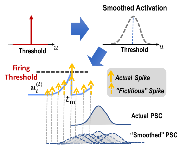
A typical strategy in dealing with the non-differentiability of the activation is to smooth the activation function by approximating it using a differentiable curve [24] as shown in the Figure 2, or a continuous probability density function [21], which is similar to the former approach in spirit. However, these approaches effectively spread each discrete firing spike continuously over time, converting one actual spike to multiple “fictitious” spikes and also generating multiple “fictitious” PSCs displaced at different time points. We stress that while smoothing circumvents the numerical challenges brought by non-differentiability of the spiking activation, it effectively alters the underlying spiking neuron model and firing times, and leads to degraded accuracy in the error gradient computation. It is important to reflect that spike timing is the hallmark of spiking neural computation, altering firing times in BP can hamper precise learning of the targeted firing sequences as pursued in this paper.
3.3.2 The Main Ideas Behind TSSL-BP
TSSL-BP addresses the two key limitations of the prior BP methods: lack proper handling of spiking discontinuities (leading to loss of temporal precision) and need for many time steps (i.e. high latency) to ensure good performance. TSSL-BP computes across two categories of spatio-temporal dependencies in the network: inter-neuron and intra-neuron dependencies. As shown in Figure 3, our key observations are: 1) temporal dependencies of a postsynaptic neuron on any of its presynaptic neurons only take place via the presynaptic spikes which generate PSCs to the postsynaptic neuron, and shall be considered as inter-neuron dependencies; 2) furthermore, the timing of one presynaptic spike affects the timing of the immediately succeeding spike from the same presynaptic neuron through the intra-neuron temporal dependency. The timing of the first presynaptic spike affects the PSC produced by the second spike, and has additional impact on the postynaptic neuron through this indirect mechanism. In the following, we show how to derive the for each neuron in layer . We denote , where represents the inter-neuron dependencies and is the intra-neuron dependencies.
3.3.3 Inter-Neuron Backpropagation
Instead of performing the problematic activation smoothing, we critically note that the all-or-none characteristics of firing behavior is such that a PSC waveform is only triggered at a presynaptic firing time. Specially, as shown in Figure 4, a perturbation of , i.e, due to weight updates, may result in an incremental shift in the firing time , which in turn shifts the onset of the PSC waveform corresponding to the shifted spike, leading to a perturbation of . We consider this as an inter-neuron dependency since the change in PSC () alters the membrane potential of the postsynaptic neuron in the next layer.

We make two important points: 1) we shall capture the inter-neuron dependencies via (the incremental changes of) the presynaptic firing times, which precisely corresponds to how different neurons interact with each other in an SNN; and 2) the inter-neuron dependency of each neuron ’s PSC at on its membrane potential at happens only if the neuron fires at . In general, ’s inter-neuron dependencies on all preceding firing times shall be considered. Figure 5 shows the situation where depends on two presynaptic firing times and . Conversely, the inter-neuron dependencies if or there is no spike at . Assuming that the presynaptic neuron spikes at , The inter-neuron dependencies is
| (11) |
where, importantly, the chain rule is applied through the presynaptic firing time .
3.3.4 Intra-Neuron Backpropagation
Now we consider the intra-neuron dependency defined between an arbitrary time and a presynaptic firing time (). From Section 3.3.3, the presynpatic firing at time invokes a continuous PSC which has a direct impact on the postsynaptic potential at time , which is an inter-neuron dependency. On the other hand, corresponds to an indirect effect on the postsynaptic potential via the intra-neuron dependency.
We consider specifically under the context of the adopted LIF model, which may occur if the presynaptic neuron spikes at immediately following such that . In this case, the presynatpic membrane potential at not only contributes to a PSC due to the neuron firing, but also affects the membrane potential at the next spike time resulted from the reset occurring at as described in (4). The PSC has an inter-neuron dependency on membrane potential while is further affected by the immediately preceding firing time due to the reset of the presynaptic potential at . Recall if neuron fires at as in (5). More precisely, takes this indirect intra-neuron effect on into consideration if and , i.e. no other presynaptic spike exists between and
| (13) |
where is the reset kernel and is evaluated by (12). In (13), would have been already computed during the backpropagation process since is a presynaptic firing time after .
Putting the inter-neuron and intra-neuron dependencies together, one of the key derivatives required in the BP process with is given by
| (14) |
where is an arbitrary time between and , and of (13) is considered.
The complete derivation of TSSL-BP is provided in Section 1 of the Supplementary Material. There are two key distinctions setting our approach apart from the aforementioned activation smoothing. First, the inter-neuron dependencies are only considered at pre-synaptic firing times as opposed to all prior time points, latter of which is the case when the activation smoothing is applied with BPTT. The handling adopted in TSSL-BP is a manifestation of the all-or-none firing characteristics of spiking neurons. Second, as in Figure 4, the key step in backpropagation is the consideration of the incremental change of spiking times, which is not considered in recent SNNs BP works.
4 Experiments and Results
We test the proposed TSSL-BP method on four image datasets MNIST [15], N-MNIST [19], FashionMNIST [26] and CIFAR10 [14]. We compare TSSL-BP with several state-of-the-art results with the same or similar network sizes including different SNNs BP methods, converted SNNs, and traditional ANNs. The details of practical simulation issues, experimental settings, and datasets preprocessing methods are described in Section 2 of the supplementary material. We have made our Pytorch implementation available online11 1 https://github.com/stonezwr/TSSL-BP. We expect this work would help move the community forward towards enabling high-performance spiking neural networks simulation within short latency.
4.1 MNIST
On MNIST [15], we compares the accuracies of the spiking CNNs trained by the TSSL-BP method with ones trained by other algorithms in Table 1. In our method, the pixel intensities of the image are converted into real-valued spike current to the inputs within a short time window. The proposed TSSL-BP delivers up to accuracy and outperforms all other methods except for the ST-RSBP [29] whose accuracy is slightly higher by . However, compared to ST-RSBP, TSSL-BP can train high-performance SNNs with only time steps, achieving reduction of step count (latency). The accuracy of [29] drops below that of TSSL-BP noticeably under short time windows. In addition, no data augmentation is applied in this experiment, which is adopted in [13] and [29].
| Methods | Network | Time steps | Epochs | Mean | Stddev | Best |
|---|---|---|---|---|---|---|
| Spiking CNN [16] | 20C5-P2-50C5-P2-200 | |||||
| STBP [24] | 15C5-P2-40C5-P2-300 | |||||
| SLAYER [21] | 12C5-p2-64C5-p2 | |||||
| HM2BP [13] | 15C5-P2-40C5-P2-300 | |||||
| ST-RSBP [29] | 15C5-P2-40C5-P2-300 | |||||
| This work | 15C5-P2-40C5-P2-300 | |||||
| 20C5: convolution layer with 20 of the filters. P2: pooling layer with filters. | ||||||
4.2 N-MNIST
We test the proposed method on N-MNIST dataset [19], the neuromorphic version of the MNIST. The inputs to the networks are spikes rather than real value currents. Table 2 compares the results obtained by different models on N-MNIST. The SNN trained by our proposed approach naturally processes spatio-temporal spike patterns, achieving the start-of-the-art accuracy of . It is important to note that our proposed method with the accuracy of outperforms the best previously reported results in [21], obtaining times fewer time steps which leads to significant latency reduction.
4.3 FashionMNIST
We compare several trained fully-connected feedforward SNNs and spiking CNNs on FashionMNIST [26], a more challenging dataset than MNIST. In Table 3, TSSL-BP achieves test accuracy on the fully-connected feedforward network of two hidden layers with each having 400 neurons, outperforming the HM2BP method of [13], which is the best previously reported algorithm for feedforward SNNs. TSSL-BP can also deliver the best test accuracy with much fewer time steps. Moreover, TSSL-BP achieves on the spiking CNN networks, noticeably outperforming the same size non-spiking CNN trained by a standard BP method.
4.4 CIFAR10
Furthermore, we apply the proposed method on the more challenging dataset of CIFAR10 [14]. As shown in Table 4, our TSSL-BP method achieves accuracy with a mean of and a standard deviation of under five trials on the first CNN and achieves accuracy on the second CNN architecture. TSSL-BP delivers the best result among a previously reported ANN, SNNs converted from pre-trained ANNs, and the spiking CNNs trained by the STBP method of [25]. CIFAR10 is a challenging dataset for most of the existing SNNs BP methods since the long latency required by those methods makes them hard to scale to deeper networks. The proposed TSSL-BP not only achieves up to accuracy improvement over the work of [25] without the additional optimization techniques including neuron normalization and population decoding which are employed in [25], but also utilizes fewer time steps.
| Methods | Network | Time steps | Epochs | Accuracy |
|---|---|---|---|---|
| Converted SNN [12] | CNN 1 | |||
| STBP [25] | CNN 1 | |||
| This work | CNN 1 | |||
| ANN [25] | CNN 2 | |||
| Converted SNN [20] | CNN 2 | 200 | ||
| STBP (without NeuNorm) [25] | CNN 2 | |||
| STBP (with NeuNorm) [25] | CNN 2 | |||
| This work | CNN 2 | |||
| CNN 1: 96C3-256C3-P2-384C3-P2-384C3-256C3-1024-1024 | ||||
| CNN 2: 128C3-256C3-P2-512C3-P2-1024C3-512C3-1024-512 | ||||
4.5 Firing Sparsity
As presented, the proposed TSSL-BP method can train SNNs with low latency. In the meanwhile, the firing activities in well-trained networks also tend to be sparse. To demonstrate firing sparsity, we select two well-trained SNNs, one for the CIFAR10 and the other for the N-MNIST.
The CIFAR10 network is simulated over time steps. We count the percentage of neurons that fire times, respectively, and average the percentages over 100 testing samples. As shown in Figure 7, the network’s firing activity is sparse. More than of neurons are silent while of neurons fire more than once, and about of neurons fire at every time step.
The N-MNIST network demonstrated here is simulated over time steps. The firing rate of each neuron is logged. The number of neurons with a certain range of firing rates is counted and averaged over 100 testing samples. Similarly, as shown in Figure 8, the firing events of the N-MNIST network are also sparse and more than of neurons keep silent. In the meanwhile, there are about of neurons with a firing rate of greater than .


5 Conclusion
We have presented the novel temporal spike sequence learning via a backpropagation (TSSL-BP) method to train deep SNNs. Unlike all prior SNNs BP methods, TSSL-BP improves temporal learning precision by circumventing the non-differentiability of the spiking activation function while faithfully reflecting the all-or-none firing characteristics and the underlying structure in the dependencies of spiking neural activities in both space and time.
TSSL-BP provides a universal BP tool for learning arbitrarily specified target firing sequences with high accuracy while achieving low temporal latency. This is in contrast with most of the existing SNN BP methods which require hundreds of time steps for achieving decent accuracy. The ability in training and inference over a few time steps results in significant reductions of the computational cost required for training large/deep SNNs, and the decision time and energy dissipation of the SNN model when deployed on either a general-purpose or a dedicated neurormorphic computing platform.
Broader Impact
Our proposed Temporal Spike Sequence Learning Backpropagation (TSSL-BP) method is able to train deep SNNs while achieving the state-of-the-art efficiency and accuracy. TSSL-BP breaks down error backpropagation across two types of inter-neuron and intra-neuron dependencies and leads to improved temporal learning precision. It captures inter-neuron dependencies through presynaptic firing times by considering the all-or-none characteristics of firing activities, and captures intra-neuron dependencies by handling the internal evolution of each neuronal state in time.
Spiking neural networks offer a very appealing biologically plausible model of computation and may give rise to ultra-low power inference and training on recently emerged large-scale neuromorphic computing hardware. Due to the difficulties in dealing with the all-or-one characteristics of spiking neurons, however, training of SNNs is a major present challenge and has limited wide adoption of SNNs models.
The potential impacts of this work are several-fold:
1) Precision: TSSL-BP offers superior precision in learning arbitrarily specified target temporal sequences, outperforming all recently developed the-state-of-the-art SNN BP methods.
2) Low latency: TSSL-BP delivers high-precision training over a very short temporal window of a few time steps. This is contrast with many BP methods that require hundreds of time steps for maintaining a decent accuracy. Low latency computation immediately corresponds to fast decision making.
3) Scalability and energy efficiency: The training of SNNs is signficantly more costly than that of the conventional neural networks. The training cost is one major bottleneck to training large/deep SNNs in order to achieve competitive performance. The low latency training capability of TSSL-BP reduces the training cost by more than one order of magnitude and also cuts down the energy dissipation of the training and inference on the deployed computing hardware.
4) Community impact: TSSL-BP has been prototyped based on the widely adopted Pytorch framework and will be made available to the public. We believe our TSSL-BP code will benefit the brain-inspired computing community from both an algorithmic and neuromorphic computing hardware development perspective.
Acknowledgments
This material is based upon work supported by the National Science Foundation (NSF) under Grants No.1948201 and No.1940761. Any opinions, findings, conclusions or recommendations expressed in this material are those of the authors and do not necessarily reflect the views of NSF, UC Santa Barbara, and their contractors.
References
- [1] Filipp Akopyan, Jun Sawada, Andrew Cassidy, Rodrigo Alvarez-Icaza, John Arthur, Paul Merolla, Nabil Imam, Yutaka Nakamura, Pallab Datta, Gi-Joon Nam, et al. Truenorth: Design and tool flow of a 65 mw 1 million neuron programmable neurosynaptic chip. IEEE Transactions on Computer-Aided Design of Integrated Circuits and Systems, 34(10):1537–1557, 2015.
- [2] Guillaume Bellec, Darjan Salaj, Anand Subramoney, Robert Legenstein, and Wolfgang Maass. Long short-term memory and learning-to-learn in networks of spiking neurons. In Advances in Neural Information Processing Systems, pages 787–797, 2018.
- [3] Guillaume Bellec, Franz Scherr, Elias Hajek, Darjan Salaj, Robert Legenstein, and Wolfgang Maass. Biologically inspired alternatives to backpropagation through time for learning in recurrent neural nets. arXiv preprint arXiv:1901.09049, 2019.
- [4] Sander M Bohte, Joost N Kok, and Han La Poutre. Error-backpropagation in temporally encoded networks of spiking neurons. Neurocomputing, 48(1-4):17–37, 2002.
- [5] Olaf Booij and Hieu tat Nguyen. A gradient descent rule for spiking neurons emitting multiple spikes. Information Processing Letters, 95(6):552–558, 2005.
- [6] Mike Davies, Narayan Srinivasa, Tsung-Han Lin, Gautham Chinya, Yongqiang Cao, Sri Harsha Choday, Georgios Dimou, Prasad Joshi, Nabil Imam, Shweta Jain, et al. Loihi: A neuromorphic manycore processor with on-chip learning. IEEE Micro, 38(1):82–99, 2018.
- [7] Peter U Diehl, Daniel Neil, Jonathan Binas, Matthew Cook, Shih-Chii Liu, and Michael Pfeiffer. Fast-classifying, high-accuracy spiking deep networks through weight and threshold balancing. In Neural Networks (IJCNN), 2015 International Joint Conference on, pages 1–8. IEEE, 2015.
- [8] Steve K Esser, Rathinakumar Appuswamy, Paul Merolla, John V Arthur, and Dharmendra S Modha. Backpropagation for energy-efficient neuromorphic computing. In Advances in Neural Information Processing Systems, pages 1117–1125, 2015.
- [9] Wulfram Gerstner and Werner M Kistler. Spiking neuron models: Single neurons, populations, plasticity. Cambridge university press, 2002.
- [10] Samanwoy Ghosh-Dastidar and Hojjat Adeli. A new supervised learning algorithm for multiple spiking neural networks with application in epilepsy and seizure detection. Neural networks, 22(10):1419–1431, 2009.
- [11] Dongsung Huh and Terrence J Sejnowski. Gradient descent for spiking neural networks. In Advances in Neural Information Processing Systems, pages 1433–1443, 2018.
- [12] Eric Hunsberger and Chris Eliasmith. Training spiking deep networks for neuromorphic hardware. arXiv preprint arXiv:1611.05141, 2016.
- [13] Yingyezhe Jin, Wenrui Zhang, and Peng Li. Hybrid macro/micro level backpropagation for training deep spiking neural networks. In Advances in Neural Information Processing Systems, pages 7005–7015, 2018.
- [14] Alex Krizhevsky, Vinod Nair, and Geoffrey Hinton. The cifar-10 dataset. online: http://www. cs. toronto. edu/ kriz/cifar.html, 2014.
- [15] Yann LeCun, Léon Bottou, Yoshua Bengio, and Patrick Haffner. Gradient-based learning applied to document recognition. Proceedings of the IEEE, 86(11):2278–2324, 1998.
- [16] Jun Haeng Lee, Tobi Delbruck, and Michael Pfeiffer. Training deep spiking neural networks using backpropagation. Frontiers in neuroscience, 10:508, 2016.
- [17] Wolfgang Maass. Networks of spiking neurons: the third generation of neural network models. Neural networks, 10(9):1659–1671, 1997.
- [18] EO Neftci, H Mostafa, and F Zenke. Surrogate gradient learning in spiking neural networks, 2019. URL https://arxiv. org/abs, 1901.
- [19] Garrick Orchard, Ajinkya Jayawant, Gregory K Cohen, and Nitish Thakor. Converting static image datasets to spiking neuromorphic datasets using saccades. Frontiers in neuroscience, 9:437, 2015.
- [20] Abhronil Sengupta, Yuting Ye, Robert Wang, Chiao Liu, and Kaushik Roy. Going deeper in spiking neural networks: Vgg and residual architectures. Frontiers in neuroscience, 13, 2019.
- [21] Sumit Bam Shrestha and Garrick Orchard. Slayer: Spike layer error reassignment in time. In Advances in Neural Information Processing Systems, pages 1412–1421, 2018.
- [22] Amirhossein Tavanaei, Masoud Ghodrati, Saeed Reza Kheradpisheh, Timothée Masquelier, and Anthony Maida. Deep learning in spiking neural networks. Neural Networks, 2018.
- [23] Paul J Werbos. Backpropagation through time: what it does and how to do it. Proceedings of the IEEE, 78(10):1550–1560, 1990.
- [24] Yujie Wu, Lei Deng, Guoqi Li, Jun Zhu, and Luping Shi. Spatio-temporal backpropagation for training high-performance spiking neural networks. Frontiers in neuroscience, 2018.
- [25] Yujie Wu, Lei Deng, Guoqi Li, Jun Zhu, Yuan Xie, and Luping Shi. Direct training for spiking neural networks: Faster, larger, better. In Proceedings of the AAAI Conference on Artificial Intelligence, volume 33, pages 1311–1318, 2019.
- [26] Han Xiao, Kashif Rasul, and Roland Vollgraf. Fashion-mnist: a novel image dataset for benchmarking machine learning algorithms. arXiv preprint arXiv:1708.07747, 2017.
- [27] Yan Xu, Xiaoqin Zeng, Lixin Han, and Jing Yang. A supervised multi-spike learning algorithm based on gradient descent for spiking neural networks. Neural Networks, 43:99–113, 2013.
- [28] Friedemann Zenke and Surya Ganguli. Superspike: Supervised learning in multilayer spiking neural networks. Neural computation, 30(6):1514–1541, 2018.
- [29] Wenrui Zhang and Peng Li. Spike-train level backpropagation for training deep recurrent spiking neural networks. In Advances in Neural Information Processing Systems, pages 7800–7811, 2019.
See pages - of supplementary.pdf