Predictive refinement methodology for compressed sensing imaging

Alfredo Nava-Tudela Thanks: Institute for Physical Science and Technology, University of Maryland, College Park, MD, USA (ant@umd.edu).

Abstract

The weak- $\ell^{p}$ norm can be used to define a measure $s$ of sparsity. When we compute $s$ for the discrete cosine transform coefficients of a signal, the value of $s$ is related to the information content of said signal. We use this value of $s$ to define a reference-free index $\mathcal{E}$ , called the sparsity index, that we can use to predict with high accuracy the quality of signal reconstruction in the setting of compressed sensing imaging. That way, when compressed sensing is framed in the context of sampling theory, we can use $\mathcal{E}$ to decide when to further partition the sampling space and increase the sampling rate to optimize the recovery of an image when we use compressed sensing techniques.

1 Introduction

In order to reproduce the voice of a singer who can sing up to a “soprano C”, or at a frequency of $W=1046$ Hz, Claude Shannon [31] proved that we need to sample her voice once every $\frac{1}{2W}$ seconds. He named this number the Nyquist sampling rate for a signal of band $W$ Hz, i.e., a signal with frequencies no higher than $W$ Hz, after Harry Nyquist, who had “pointed out the fundamental importance of the time interval $\frac{1}{2W}$ in connection with telegraphy.”

Shannon notes that this result was known in other forms by the mathematician J. M. Whittaker [34], but that otherwise had not appeared explicitly in the literature of communication theory. The idea must have been in the air since Nyquist [24]; Bennett [4], in the steady state case; and Gabor [16] had pointed out that approximately $2TW$ numbers are sufficient to capture a signal of band $W$ Hz that lasts for $T$ seconds.

Further in “Communication in the presence of noise” [31], published a year after his seminal “A mathematical theory of communication” [30], Shannon establishes a method to represent geometrically any communication system, and explores the utility of mapping a sequence of samples of a band limited signal into a high dimensional vector space. And it is here where he makes the most interesting of all remarks, on page 13: “[…] in the case of speech, the ear is insensitive to a certain amount of phase distortion. Messages differing only in the phases of their components […] sound the same. This may have the effect of reducing the number of essential dimensions in the message space.”

In other words, even if the dimension of the ambient vector space where we embed a representation of a signal is very high, we may come up with an equivalence class for which member points will have similar information content as the original signal, as far as the end user is concerned; and that equivalence class, in turn, will induce a low dimensional manifold in the vector space where similar messages can be mapped.

These ideas make it natural to frame the theory of compressed sensing [10, 9, 13, 7, 20] in the context of sampling and information theories. To see this, observe that compressed sensing makes it possible to reconstruct a signal, under certain circumstances, with fewer measurements than the otherwise required number of samples dictated by the Nyquist sampling rate. Moreover, even when the reconstruction is not exact, the error will be small.

In specific, compressed sensing deals with the problem of recovering a signal or message of interest $\mathbf{v}\in\mathbb{R}^{n}$ , which we assume can be represented as $\mathbf{v}=\mathbf{A}\mathbf{x}$ for a matrix $\mathbf{A}\in\mathbb{R}^{n\times N}$ , with $n\leq N$ , from an incomplete set of linear measurements,

\mathbf{b}=\Phi\mathbf{x},

(1)

where $\mathbf{b}\in\mathbb{R}^{m}$ is the vector of measurements, $\mathbf{x}\in\mathbb{R}^{N}$ is the object to recover, and $\Phi\in\mathbb{R}^{m\times N}$ is the measurement matrix, with $m<n$ and $\Phi$ is a full rank matrix.¹¹ 1 If $n=N$ , we are in the setting of transform coding, where $\mathbf{A}$ represents a unitary transform, for example; and if $n<N$ , we can talk of a dictionary or a frame representation of $\mathbf{v}$ . Given a measurement vector $\mathbf{b}$ , eq. 1 represents an underdetermined system of linear equations, with an infinite number of solutions. However, if $\mathbf{x}$ has at most $k\leq m$ significant components, compared to the rest, we can recover it exactly, or very closely, by solving the constrained problem,

\min_{\mathbf{x}\in\mathbb{R}^{N}}f(\mathbf{x})\quad\text{subject to }\|\mathbf{b}-\Phi\mathbf{x}\|_{2}=0,

(2)

where $f(\cdot)=\|\cdot\|_{d}$ , and $d=0\text{ or }1$ . Here $\|\mathbf{x}\|_{0}$ counts the number of nonzero entries of $\mathbf{x}$ . If $\mathbf{x}^{\star}$ is a solution to eq. 2, we then synthesize an approximate reconstruction of $\mathbf{v}$ by using $\mathbf{A}\mathbf{x}^{\star}$ .

Note that since $m<n$ , we have used fewer measurements than the number of coordinates of $\mathbf{v}$ , in effect compressing the sensing, hence the name compressed sensing; possibly beating the Nyquist sampling rate; going from a large dimensional message space, $\mathbb{R}^{n}$ , to a smaller dimensional measurement space, $\mathbb{R}^{m}$ , in a manner that hopefully captures the essence of the signal of interest. Just like Shannon envisioned.

For all of this to work, we need to make precise the notion of what the “significant components” of $\mathbf{x}$ are, notion which traditionally has translated into talking of sparsity. However, we show in example 1 that the commonly used notion of sparsity—the number of nonzero entries in a vector—is defective, and we propose instead in section 2 a refined notion $s$ of sparsity that extends the traditional meaning of the word as used in the compressed sensing and sparse representation literatures. The definition of $s$ is based on the weak- $\ell^{p}$ norm, which we define and study in section 2.1. The weak- $\ell^{p}$ norm helps us define, for a given $0<p\leq 1$ , the sparsity function $s_{p}:\mathbb{R}^{n}\rightarrow\mathbb{R}$ and the sparsity relation $<_{s_{p}}$ , which induces a strict partial order on $\mathbb{R}^{n}$ . We show that, for a given vector $\mathbf{x}\in\mathbb{R}^{n}$ , $s_{p}(\mathbf{x}):\mathbb{R}\rightarrow\mathbb{R}$ is a convex function of $p$ , and we use this fact to compute effectively $\inf_{p\in(0,1]}s_{p}(\mathbf{x})$ , which we define as the sparsity $s(\mathbf{x})$ of $\mathbf{x}$ . See section 2.2.

In section 2.3 we study unitary transformations and the sparsity $s$ , which we use to define sparsifying transforms and their properties, formalizing well known energy shifting properties of unitary transforms commonly used in compression, for example. This leads in section 2.4 to the study of error analysis and sparsity $s$ when we truncate the signal representation $\mathbf{x}$ of a vector $\mathbf{v}$ under a sparsifying unitary transform $\mathbf{T}$ . This is done in terms of the peak signal-to-noise ratio or PSNR, for which we find a lower bound in terms of $s$ .

This error analysis and musings on information theoretical matters in appendix A motivate the definition of the sparsity index $\mathcal{E}$ in section 2.5, which we use in the context of compressed sensing image reconstruction, by example of the single pixel camera, which is described in detail in section 3: In section 3.1 we provide background on the origin of the single pixel camera, in section 3.2 we provide a physical realization and mathematical modeling of a single pixel camera, and how to go about obtaining an image from it both in an inefficient way, section 3.2.1, and the compressed sensing way, section 3.2.2. In section 3.3 we show how to solve the single pixel camera compressed sensing problem with either the orthogonal matching pursuit algorithm (OMP), section 3.3.1, or the more efficient and better basis pursuit algorithm (BP), section 3.3.2, for which, in appendix B, we provide the specific methods that we use to implement it. The characteristics of OMP help us tie in the use of the sparsity index $\mathcal{E}$ with the calculation of a lower bound of the PSNR of the various compressed sensing image reconstructions conducted in section 4 with BP, given that the solutions obtained with OMP and BP are close. Our results show that we can predict the quality of the reconstruction of images with very good accuracy without knowledge of the original, i.e., we show that we have in the sparsity index $\mathcal{E}$ a reference-free tool to decide when to sample at a higher rate a given region to guarantee a minimum local PSNR reconstruction.

2 Sparsity

In this section we define the weak- $\ell^{p}$ norm, go over some of its properties, and use it to redefine the notion of sparsity, which in common parlance refers to the counting of nonzero entries in a vector. We do this because we show with an example why the commonly used notion of sparsity is not fully satisfactory, and propose instead a new measure of sparsity that utilizes the weak- $\ell^{p}$ norm, mentioned as a measure of sparsity in [6], and used in that capacity in, for example, [12] and [8]. We then derive some properties of this measure of sparsity.

2.1 The weak- $\ell^{p}$ norm and its properties

It is easy to see that given a vector $\mathbf{x}=(x_{1},x_{2},\ldots,x_{n})^{\text{T}}\in\mathbb{R}^{n}$ , there exists a unique vector $\mathbf{y}=(y_{1},y_{2},\ldots,y_{n})^{\text{T}}\in\mathbb{R}^{n}$ satisfying the following two properties:

1.

For all $i\in\{1,2,\ldots,n\}$ , there is a $j\in\{1,2,\ldots,n\}$ such that $|x_{i}|=y_{j}$ , and
2.

For all $i,j\in\{1,2,\ldots,n\}$ we have that $y_{i}\leq y_{j}\Leftrightarrow i\leq j$ .

These two properties naturally define the ordering operator $\Omega:\mathbb{R}^{n}\rightarrow\mathbb{R}^{n}$ , which assigns to $\mathbf{x}$ its corresponding $\mathbf{y}$ . We then write $\mathbf{y}=\Omega(\mathbf{x})$ , and say that $\mathbf{y}$ is the ordering of $\mathbf{x}$ .

Definition 1 (Weak- $\ell^{p}$ norm)

Let $\mathbf{x}\in\mathbb{R}^{n}$ and $p>0$ . We define the weak- $\ell^{p}$ norm of vector $\mathbf{x}$ as the number

\|\mathbf{x}\|_{w\ell^{p}}=\left(\sup_{\epsilon>0}N(\epsilon,\mathbf{x})\epsilon^{p}\right)^{\frac{1}{p}},

where $N(\epsilon,\mathbf{x})=\#\{j:|x_{j}|>\epsilon\}$ .

We are interested in the weak- $\ell^{p}$ norm because for values of $p\in(0,1]$ , for a given vector $\mathbf{x}$ , the quantity $\|\mathbf{x}\|_{w\ell^{p}}^{p}$ can be used as a measure of sparsity of $\mathbf{x}$ . We elaborate on this later on. First, we address how to effectively compute $\|\cdot\|_{w\ell^{p}}$ .

Theorem 1

Given a vector $\mathbf{x}\in\mathbb{R}^{n}$ , and $p>0$ , we have that

\|\mathbf{x}\|_{w\ell^{p}}^{p}=\max_{i}\#\{j:y_{j}\geq y_{i}\}y_{i}^{p},

(3)

where $\mathbf{y}=(y_{1},y_{2},\ldots,y_{n})^{\text{T}}=\Omega(\mathbf{x})$ . We define the index $i_{\star}=i_{\star}(\mathbf{x},p)$ as the smallest index where the right hand side of eq. 3 reaches its maximum.

Proof 1

The statement is trivially true for $\mathbf{x}=\mathbf{0}$ . Assume then that $\mathbf{x}$ is a nonzero vector with corresponding ordering $\mathbf{y}=\Omega(\mathbf{x})$ . First observe that, for a given $\epsilon>0$ , the order in which we count the number of entries $x_{j}$ in $\mathbf{x}$ that are greater in absolute value than $\epsilon$ , does not depend on said order. Therefore, for a given $\epsilon>0$ , we have that $N(\epsilon,\mathbf{x})=\#\{j:|x_{j}|>\epsilon\}=\#\{j:y_{j}>\epsilon\}=N(\epsilon,\mathbf{y})$ .

Since $\mathbf{x}\neq\mathbf{0}$ , there is an integer $i\in\{1,2,\ldots,n\}$ such that $y_{i}>0$ . Let $i_{0}$ be the smallest of such integers. Consider the following partition $\cal{P}$ of $(0,+\infty)=(0,y_{i_{0}})\cup[y_{i_{0}},y_{i_{0}+1})\cup\ldots\cup[y_{n},\infty)$ . We compute the supremum of $N(\epsilon,\mathbf{y})\epsilon^{p}$ over each of the intervals defining $\cal{P}$ . For $\epsilon\in(0,y_{i_{0}})=I_{0}$ , we have that $N(\epsilon,\mathbf{y})=n-i_{0}+1$ , and since raising a number to the $p^{\text{th}}$ power is a monotonically increasing operation, we clearly have that $\sup_{\epsilon\in I_{0}}N(\epsilon,\mathbf{y})\epsilon^{p}=(n-i_{0}+1)y_{i_{0}}^{p}=\#\{j:y_{j}\geq y_{i_{0}}\}y_{i_{0}}^{p}$ . Similarly, for $\epsilon\in[y_{i_{0}+k},y_{i_{0}+k+1})=I_{k+1}$ , we have that $\sup_{\epsilon\in I_{k+1}}N(\epsilon,\mathbf{y})\epsilon^{p}=\#\{j:y_{j}\geq y_{i_{0}+k+1}\}y_{i_{0}+k+1}^{p}$ . Finally, for $\epsilon\in[y_{n},\infty)=I_{\infty}$ , we have that $N(\epsilon,\mathbf{y})=0$ , and therefore $\sup_{\epsilon\in I_{\infty}}N(\epsilon,\mathbf{y})\epsilon^{p}=0$ . The result follows from observing that the supremum of $N(\epsilon,\mathbf{y})\epsilon^{p}$ over $(0,\infty)$ is the maximum of the supremums of $N(\epsilon,\mathbf{y})\epsilon^{p}$ over each and all of the intervals $I_{0},I_{1},\ldots,I_{n-i_{0}},I_{\infty}$ .

We state without proof the following properties of the weak- $\ell^{p}$ norm, derived from theorem 1.

Theorem 2

Let $\mathbf{x}\in\mathbb{R}^{n}$ , $\alpha\in\mathbb{R}$ , and $p>0$ . Then

1.

$\|\mathbf{x}\|_{w\ell^{p}}\geq 0$ .
2.

$\|\mathbf{x}\|_{w\ell^{p}}=0$ if and only if $\mathbf{x}=\mathbf{0}$ .
3.

$\|\alpha\mathbf{x}\|_{w\ell^{p}}=|\alpha|\|\mathbf{x}\|_{w\ell^{p}}$ .
4.

The weak- $\ell^{p}$ norm does not satisfy the triangle inequality.
5.

$\|\mathbf{x}\|_{w\ell^{p}}\leq\|\mathbf{x}\|_{p}$ , where $\|\mathbf{x}\|_{p}=(\sum_{i}|x_{i}|^{p})^{\frac{1}{p}}$ is the $\ell^{p}$ -norm.

Therefore, the weak- $\ell^{p}$ norm, is not a true norm, but almost. It is a quasi norm, but for simplicity we will refer to it as a “norm”. We explore and get acquainted with two more properties of the weak- $\ell^{p}$ norm that will be relevant later on.

From the result of theorem 1, we observe that the $p^{\text{th}}$ power of the weak- $\ell^{p}$ norm of a vector $\mathbf{x}\in\mathbb{R}^{n}$ corresponds to the largest area of a rectangle of width $\#\{j:y_{j}\geq y_{i}\}=n-i+1$ , and height $y_{i}^{p}$ , where $\mathbf{y}=\Omega(\mathbf{x})$ . Recall that in theorem 1 we defined $i_{\star}$ to be the smallest index for which this maximal area is achieved since we will use $i_{\star}$ often. For a graphic representation of this concept, see figs. 1 and 2.

Note that for any value of $p>0$ , for a given $i\in\{1,2,\ldots,n\}$ , $\#\{j:y_{j}\geq y_{i}\}=n-i+1$ ; while $\lim_{p\rightarrow 0^{+}}y_{i}^{p}$ tends to either 1 or 0, depending on whether $y_{i}\neq 0$ or $y_{i}=0$ , respectively, i.e., $y_{i}^{p}$ tends to the characteristic function $\chi_{\mathbb{R}^{*}}$ as $p$ goes to zero. Here $\mathbb{R}^{*}=\mathbb{R}\setminus\{0\}$ . It follows that

\lim_{p\rightarrow 0^{+}}\#\{j:y_{j}\geq y_{i}\}y_{i}^{p}=\begin{cases}n-i+1,&\text{if }y_{i}\neq 0,\\ 0,&\text{if }y_{i}=0.\end{cases}

We conclude from the previous two paragraphs that

\lim_{p\rightarrow 0^{+}}\|\mathbf{x}\|_{w\ell^{p}}^{p}=\|\mathbf{x}\|_{0}:=\#\{j:x_{j}\neq 0\}.

(4)

Hence, in the case when $p\rightarrow 0^{+}$ , the weak- $\ell^{p}$ norm tends to the $\ell_{0}$ -norm, which counts the nonzero entries of a vector, as defined in eq. 4. Note that the $\ell_{0}$ -norm is not a norm either, since $\|\alpha\mathbf{x}\|_{0}\neq|\alpha|\|\mathbf{x}\|_{0}$ for $\alpha\in\mathbb{R}^{*}$ when $\mathbf{x}\neq\mathbf{0}$ , but it is commonly called a “norm” nonetheless.

However, the $\ell_{0}$ -norm is not nuanced at all when we are trying to measure sparsity, usually defined as the count of the nonzero entries of a vector, in cases where a vector $\mathbf{x}\in\mathbb{R}^{n}$ has relatively few entries that are considerably larger than the rest in absolute value, a circumstance which we would like to distinguish for reasons that will become clear later on. With this in mind, we propose a new definition and measure of sparsity next.

Refer to caption — Figure 1: Graph of the $p^{\text{th}}$ power of the entries $y_{i}$ of $\mathbf{y}=\Omega(\mathbf{x})$ versus $i$ . The red circle marks the point $(i_{\star},y_{i_{\star}}^{p})$ , for $p=\frac{1}{4}$ , in this case. See theorem 1 for the definition of $i_{\star}$ .

2.2 Defining and measuring sparsity

In common parlance, as we mentioned in section 2.1, we say that a vector $\mathbf{x}=(x_{1},x_{2},\ldots,x_{n})^{\text{T}}\in\mathbb{R}^{n}$ is sparse if its $\ell_{0}$ -norm is smaller than $n$ . In other words,

\|\mathbf{x}\|_{0}=\#\{j:x_{j}\neq 0\}<n.

(5)

As argued above, though, this measure of sparsity will not distinguish the following two vectors in $\mathbb{R}^{5}$ as radically different:

Example 1

Consider $\mathbf{x}_{1}=(1,1,1,1,0)^{\text{T}}$ and $\mathbf{x}_{2}=(2,10^{-16},10^{-16},10^{-16},0)^{\text{T}}$ . From the $\ell_{0}$ -norm point of view, they are both sparse, moreover, their $\ell_{0}$ -norms are equal, yet, most of the entries of $\mathbf{x}_{1}$ are 1, while most of the entries of $\mathbf{x}_{2}$ are practically 0.

Clearly, the notion of sparsity defined by eq. 5 cannot distinguish the very different nature of these two vectors, $\mathbf{x}_{1}$ and $\mathbf{x}_{2}$ .

Note that in the example above, we deliberately chose both vectors to have approximately equal energy, if we define the energy of a vector $\mathbf{x}$ as $\|\mathbf{x}\|_{2}^{2}=\sum_{i}x_{i}^{2}$ . With these observations in hand, we put forth the following definitions.

Definition 2 (Sparsity $s_{p}$ and sparsity relation $<_{s_{p}}$ )

Let $p\in(0,1]$ . Consider the set $X=\mathbb{R}^{n}$ , and define the binary relation $R\subset X\times X$ as follows:

\text{For all }\mathbf{x}_{1},\mathbf{x}_{2}\in X,\text{ if }\|\mathbf{x}_{1}\|_{2}=\|\mathbf{x}_{2}\|_{2}\text{ and }\|\mathbf{x}_{1}\|_{w\ell^{p}}<\|\mathbf{x}_{2}\|_{w\ell^{p}},\text{ then }(\mathbf{x}_{1},\mathbf{x}_{2})\in R.

We call $R$ the sparsity relation (for $\mathbb{R}^{n}$ of order $p$ ), and will write for simplicity $\mathbf{x}_{1}<_{s_{p}}\mathbf{x}_{2}$ whenever $(\mathbf{x}_{1},\mathbf{x}_{2})\in R$ . If $\mathbf{x}_{1}<_{s_{p}}\mathbf{x}_{2}$ , we say that $\mathbf{x}_{1}$ is sparser than $\mathbf{x}_{2}$ . We say that $\mathbf{x}\in X$ has sparsity of order $p$ equal to $s_{p}(\mathbf{x}):=\|\mathbf{x}\|_{w\ell^{p}}^{p}$ , or simply, that $\mathbf{x}$ has sparsity $s_{p}(\mathbf{x})$ .

Theorem 3

Let $p\in(0,1]$ , then $(\mathbb{R}^{n},<_{s_{p}})$ is a strict partially ordered set.

Proof 2

Let $p\in(0,1]$ . For all $\mathbf{x}\in\mathbb{R}^{n}$ , we have that $<_{s_{p}}$ is trivially irreflexive, i.e., $\mathbf{x}\not<_{s_{p}}\mathbf{x}$ , since $\|\mathbf{x}\|_{w\ell^{p}}=\|\mathbf{x}\|_{w\ell^{p}}$ , hence $\mathbf{x}\not<_{s_{p}}\mathbf{x}$ . Let $\mathbf{x}_{1},\mathbf{x}_{2},\mathbf{x}_{3}\in\mathbb{R}^{n}$ and assume that $\mathbf{x}_{1}<_{s_{p}}\mathbf{x}_{2}$ and $\mathbf{x}_{2}<_{s_{p}}\mathbf{x}_{3}$ . Then, by definition, we must have that $\|\mathbf{x}_{1}\|_{2}=\|\mathbf{x}_{2}\|_{2}$ and $\|\mathbf{x}_{2}\|_{2}=\|\mathbf{x}_{3}\|_{2}$ , as well as $\|\mathbf{x}_{1}\|_{w\ell^{p}}<\|\mathbf{x}_{2}\|_{w\ell^{p}}$ and $\|\mathbf{x}_{2}\|_{w\ell^{p}}<\|\mathbf{x}_{3}\|_{w\ell^{p}}$ , since both $=$ and $<$ are transitive in $\mathbb{R}$ , we have that $\|\mathbf{x}_{1}\|_{2}=\|\mathbf{x}_{3}\|_{2}$ and $\|\mathbf{x}_{1}\|_{w\ell^{p}}<\|\mathbf{x}_{3}\|_{w\ell^{p}}$ , and therefore $\mathbf{x}_{1}<_{s_{p}}\mathbf{x}_{3}$ , i.e., $<_{s_{p}}$ is transitive.

When we have a partially ordered set, e.g., $(\mathbb{R}^{n},<_{s_{p}})$ , we are usually interested in knowing if there are maximal or minimal elements in it with respect to its ordering. Assuming the Axiom of Choice in the form of Zorn’s lemma—which states that a partially ordered set in which every chain (i.e., every totally ordered subset), has an upper (lower) bound, necessarily contains at least one maximal (minimal) element—we would then set to find upper (lower) bounds in $\mathbb{R}^{n}$ for each energy level to conclude that there exist maximal (minimal) elements in $\mathbb{R}^{n}$ with respect to the partial order $<_{s_{p}}$ . We leave the task of establishing the existence of maximal or minimal elements in $(\mathbb{R}^{n},<_{s_{p}})$ for another occasion, since this departs from the focus of our endeavors.

Note that the proof of theorem 3 does not use anywhere that $p\in(0,1]$ and is, in fact, true for any $p>0$ . However, given the aforementioned observations stemming from eq. 4 and eq. 5, it is clear that measuring sparsity with $s_{p}$ and comparing the sparsity of two vectors with the sparsity relation $<_{s_{p}}$ , are meaningful and sensible concepts only when $p\in(0,1]$ . Therefore, going forward, we will assume that $p\in(0,1]$ , unless otherwise noted.

Theorem 4 (Convexity of $s_{p}$ as a function of $p$ )

For all $\mathbf{x}\in\mathbb{R}^{n}$ , the function $f_{\mathbf{x}}:(0,1]\rightarrow\mathbb{R}$ that maps $p\mapsto s_{p}(\mathbf{x})$ is a convex function. Moreover, if $\mathbf{y}=(y_{1},y_{2},\ldots,y_{n})^{\text{T}}=\Omega(\mathbf{x})$ is the ordering of $\mathbf{x}$ and $\mathcal{I}_{\star}(\mathbf{x})=\{i_{\star}(\mathbf{x},p):p\in(0,1]\}$ is such that $\{y_{i}:i\in\mathcal{I}_{\star}(\mathbf{x})\}\cap\{0,1\}=\emptyset$ , then $f_{\mathbf{x}}$ is strictly convex. (See theorem 1 for the definition of $i_{\star}$ .)

Proof 3

Let $\mathbf{x}\in\mathbb{R}^{n}$ , $p_{1},p_{2}\in(0,1]$ , $p_{1}\neq p_{2}$ , and $t\in[0,1]$ . We have that, by theorem 1,

$\displaystyle f_{\mathbf{x}}(tp_{1}+(1-t)p_{2})$	$\displaystyle=s_{tp_{1}+(1-t)p_{2}}(\mathbf{x}),$
	$\displaystyle=\\|\mathbf{x}\\|_{w\ell_{tp_{1}+(1-t)p_{2}}}^{tp_{1}+(1-t)p_{2}},$
	$\displaystyle=\max_{i}\#\{j:y_{j}\geq y_{i}\}y_{i}^{tp_{1}+(1-t)p_{2}},$
	$\displaystyle=\max_{i}\#\{j:y_{j}\geq y_{i}\}y_{i}^{tp_{1}}y_{i}^{(1-t)p_{2}},$	(6)

where $\mathbf{y}=\Omega(\mathbf{x})$ is the ordering of $\mathbf{x}$ . If we prove that, for all $i\in\mathcal{I}_{\star}(\mathbf{x})$ ,

y_{i}^{tp_{1}}y_{i}^{(1-t)p_{2}}\leq ty_{i}^{p_{1}}+(1-t)y_{i}^{p_{2}},

(7)

combining 3 and eq. 7, it follows that,

$\displaystyle\max_{i}\#\{j:y_{j}\geq y_{i}\}y_{i}^{tp_{1}}y_{i}^{(1-t)p_{2}}$	$\displaystyle\leq\max_{i}\#\{j:y_{j}\geq y_{i}\}\left(ty_{i}^{p_{1}}+(1-t)y_{i}^{p_{2}}\right),$	(8)
	$\displaystyle\leq\max_{i}\#\{j:y_{j}\geq y_{i}\}ty_{i}^{p_{1}}+\max_{k}\#\{j:y_{j}\geq y_{k}\}(1-t)y_{k}^{p_{2}},$
	$\displaystyle=ts_{p_{1}}(\mathbf{x})+(1-t)s_{p_{2}}(\mathbf{x})=tf_{\mathbf{x}}(p_{1})+(1-t)f_{\mathbf{x}}(p_{2}),$

proving that $f_{\mathbf{x}}$ is convex. Hence, we proceed to prove eq. 7. Let $a,b\in\mathbb{R}$ , and define the functions $g(t)=e^{ta+(1-t)b}$ and $h(t)=te^{a}+(1-t)e^{b}$ . We then have that,

	$\displaystyle g(0)=e^{b},h(0)=e^{b},$
	$\displaystyle g(1)=e^{a},h(1)=e^{a}.$

That is, both functions coincide at values $t=0,1$ . Noting that the graph of $h$ is a line, and observing that $g^{\prime\prime}(t)=(a-b)^{2}e^{ta+(1-t)b}\geq 0$ , it follows that $g$ is convex, and conclude that $g(t)\leq h(t)$ for all $t\in[0,1]$ . Setting $a=\ln(y_{i}^{p_{1}})$ and $b=\ln(y_{i}^{p_{2}})$ , we get that for $t\in[0,1]$ ,

	$\displaystyle g(t)\leq h(t)\quad\Rightarrow\quad$	$\displaystyle e^{t\ln(y_{i}^{p_{1}})+(1-t)\ln{y_{i}^{p_{2}}}}\leq te^{\ln(y_{i}^{p_{1}})}+(1-t)e^{\ln(y_{i}^{p_{2}})},$
	$\displaystyle\Leftrightarrow\quad$	$\displaystyle y_{i}^{tp_{1}}y_{i}^{(1-t)p_{2}}\leq ty_{i}^{p_{1}}+(1-t)y_{i}^{p_{2}},$		(9)

proving that eq. 7 holds, as required to complete the first half of the proof. For the second half of the claim, simply note that if $\mathcal{I}_{\star}(\mathbf{x})$ is such that $\{y_{i}:i\in\mathcal{I}_{\star}(\mathbf{x})\}\cap\{0,1\}=\emptyset$ , eqs. 7, 8 and 3 become strict inequalities, resulting then in strict convexity for $f_{\mathbf{x}}$ .

Definition 3 (Sparsity $s$ )

We define the sparsity $s$ as the function $s:\mathbb{R}^{n}\rightarrow\mathbb{R}$ that assigns to every vector $\mathbf{x}\in\mathbb{R}^{n}$ the number

s(\mathbf{x})=\inf_{p\in(0,1]}s_{p}(\mathbf{x}).

To check that $s$ is well defined, we simply need to prove that for every vector $\mathbf{x}\in\mathbb{R}^{n}$ , $s(\mathbf{x})\in\mathbb{R}$ . Let $p\in(0,1]$ . Then, from theorem 2 and definition 2, we have that

0\leq s_{p}(\mathbf{x})=\|\mathbf{x}\|_{w\ell^{p}}^{p}\leq\|\mathbf{x}\|_{p}^{p}<\infty,

hence the set $\{s_{p}(\mathbf{x}):p\in(0,1]\}$ is bounded and, therefore, the number $\inf_{p\in(0,1]}s_{p}(\mathbf{x})$ exists and is unique, which means that $s$ is well defined. Moreover, in light of theorem 4, computing $s$ can be easily achieved by convex minimization techniques.

It is easy to see that $s$ has the following properties, which we state without proof.

Theorem 5

Let $\mathbf{x}\in\mathbb{R}^{n}$ , and $\mathbf{y}=(y_{1},y_{2},\ldots,y_{n})^{\text{T}}=\Omega(\mathbf{x})$ its ordering. Then,

1.

$0\leq s(\mathbf{x})\leq\|\mathbf{x}\|_{0}$ .
2.

If $\mathbf{y}$ is such that $\mathbf{y}\in Diag(\mathbb{R}^{n})=\{\mathbf{c}\in\mathbb{R}^{n}:\mathbf{c}=(c,c,\ldots,c)^{\text{T}},c\in\mathbb{R}\}$ , i.e., the ordering of $\mathbf{x}$ is a vector in the diagonal of $\mathbb{R}^{n}$ , then

$s(\mathbf{x})=\begin{cases}n,&\text{if }c\geq 1,\\ cn,&\text{if }c<1,\end{cases}$

where $\mathbf{y}=(c,c,\ldots,c)^{\text{T}}$ . Recall that, by definition of $\mathbf{y}$ , we must have $c\geq 0$ .
3.

If $\mathbf{y}$ is such that $y_{1}\geq 1$ , then $s(\mathbf{x})=n$ .

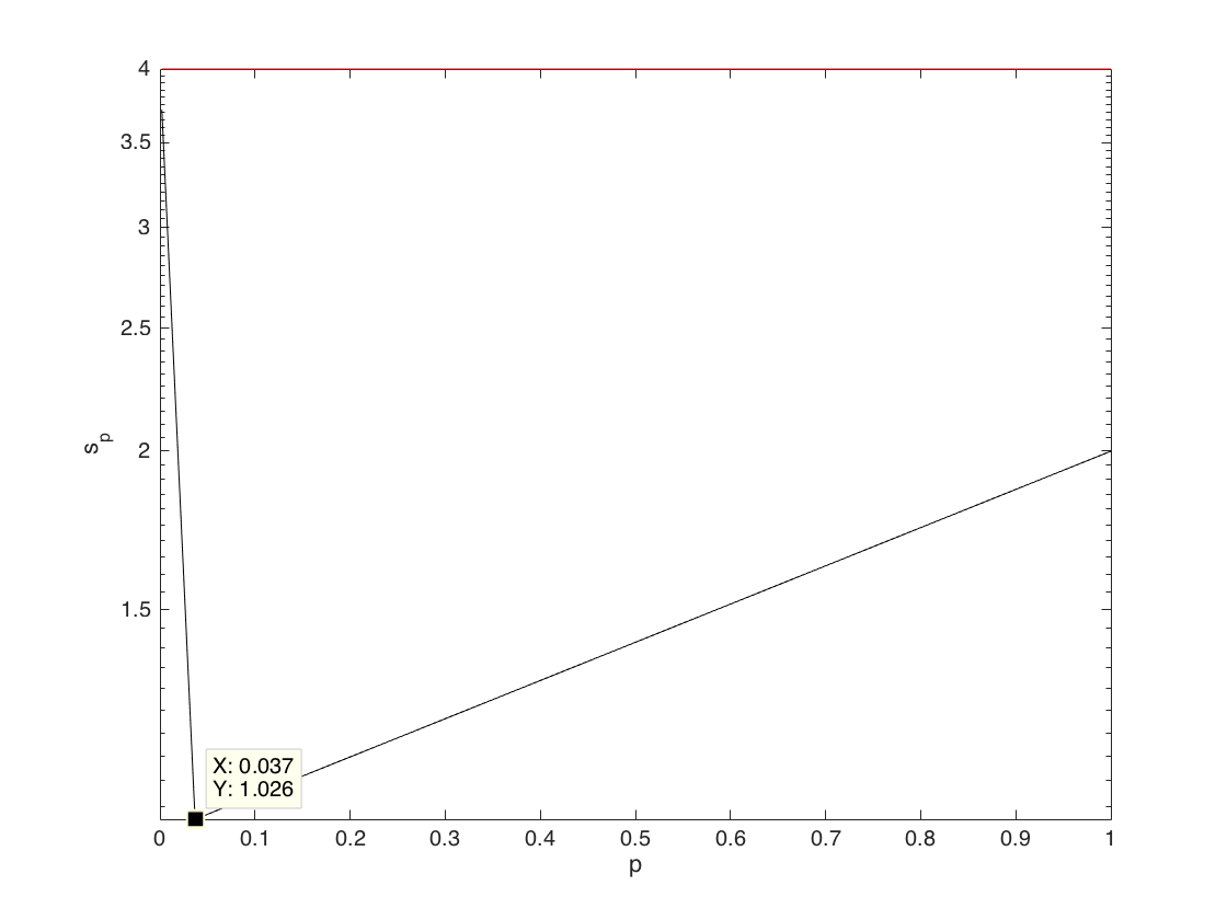
With this new definition of sparsity in hand, we revisit example 1 by computing $s(\mathbf{x}_{1})$ and $s(\mathbf{x}_{2})$ , recalling that $\mathbf{x}_{1}=(1,1,1,1,0)^{\text{T}}$ and $\mathbf{x}_{2}=(2,10^{-16},10^{-16},10^{-16},0)^{\text{T}}$ . This calculation requires from us to compute $s_{p}(\cdot)$ repeatedly, for which we refer the reader to theorem 1 on how to do it from now on.

We have that $s_{p}(\mathbf{x}_{1})=\max\{5\times 0^{p},4\times 1^{p}\}=4$ , and therefore $s(\mathbf{x}_{1})=4$ , which, we note, is equal to $\|\mathbf{x}_{1}\|_{0}$ . Now for $s(\mathbf{x}_{2})$ , we have that $s_{p}(\mathbf{x}_{2})=\max\{5\times 0^{p},4\times 10^{-16p},1\times 2^{p}\}$ . If we draw the graph of $s_{p}(\mathbf{x}_{2})$ as a function of $p$ , we see that it is the union of two curves $\Gamma_{1}$ and $\Gamma_{2}$ , with $\Gamma_{1}=\left\{(p,4\times 10^{-16p})\in\mathbb{R}^{2}:p\in(0,p_{0}]\right\}$ and $\Gamma_{2}=\left\{(p,2^{p})\in\mathbb{R}^{2}:p\in[p_{0},1]\right\}$ , where $p_{0}$ is the abscissa such that $4\times 10^{-16p_{0}}=2^{p_{0}}$ , readily seen as the minimum of $s_{p}(\mathbf{x}_{2})$ over $p\in(0,1]$ . It is easy to compute that $p_{0}=\frac{\ln(4)}{\ln(2)+16\ln(10)}\approx 0.036934$ , from which $s(\mathbf{x}_{2})\approx 1.025931$ , faithfully reflecting the fact that most of the entries in $\mathbf{x}_{2}$ are practically zero, except for one of them, which is distinctly nonzero. See fig. 3.

2.3 Unitary transforms and sparse representations

In this section we use our new definition of sparsity to explore unitary transforms and sparse representations stemming from them, which we define next.

Definition 4 (Sparsifying transform and sparse representation)

Let $\mathbf{T}\in\mathbb{R}^{n\times n}$ be a unitary matrix, and consider the transform $T:\mathbb{R}^{n}\rightarrow\mathbb{R}^{n}$ that assigns to every vector $\mathbf{v}\in\mathbb{R}^{n}$ the vector $T(\mathbf{v})=\mathbf{T}\mathbf{v}=\mathbf{x}$ . We say that $T$ is a sparsifying transform for $V\subset\mathbb{R}^{n}$ if and only if for every vector $\mathbf{v}\in V$ , we have that

\mathbf{x}<_{s_{p}}\mathbf{v},\quad\text{for all }p\in(0,1].

In this case we say that $\mathbf{T}$ is a sparsifying matrix for $V$ , $\mathbf{x}$ is a sparse representation of $\mathbf{v}$ (under $\mathbf{A}=\mathbf{T}^{-1}=\mathbf{T}^{\text{T}}$ ), and $\mathbf{v}$ admits ( $\mathbf{x}$ as) a sparse representation (under $\mathbf{A}=\mathbf{T}^{-1}=\mathbf{T}^{\text{T}}$ ).

Note that the notion of a sparsifying transform is well defined since it applies to unitary matrices, which preserve energy, i.e., $\|\mathbf{v}\|_{2}^{2}=\|\mathbf{T}\mathbf{v}\|_{2}^{2}$ for all $\mathbf{v}\in\mathbb{R}^{n}$ , and therefore $\mathbf{x}=\mathbf{T}\mathbf{v}$ and $\mathbf{v}$ can be compared by the sparsity relation $<_{s_{p}}$ , see definition 2.

Theorem 6 (Sparsity and energy distribution)

Let $\mathbf{T}\in\mathbb{R}^{n\times n}$ be a sparsifying matrix for $V\subset\mathbb{R}^{n}$ , and let $\mathbf{v}\in V$ be a vector whose transform is $\mathbf{x}=\mathbf{T}\mathbf{v}$ . If $\mathbf{y}=\Omega(\mathbf{x})$ and $\mathbf{w}=\Omega(\mathbf{v})$ are the orderings of $\mathbf{x}$ and $\mathbf{v}$ , respectively, then there exists an integer $i_{\natural}$ such that $y_{i_{\natural}}<w_{i_{\natural}}$ and $y_{i}\geq w_{i}$ for all $i>i_{\natural}$ . Moreover,

\sum_{i\leq i_{\natural}}y_{i}^{2}\leq\sum_{i\leq i_{\natural}}w_{i}^{2}\quad\text{and}\quad\sum_{i>i_{\natural}}w_{i}^{2}\leq\sum_{i>i_{\natural}}y_{i}^{2}.

(10)

Proof 4

Let $p\in(0,1]$ , and $\mathbf{v}\in V$ . Since $\mathbf{T}$ is sparsifying for $V$ , we have, by definition 4, that $s_{p}(\mathbf{x})<s_{p}(\mathbf{v})$ , from which, by theorem 1,

(n-i_{\star}(\mathbf{v},p)+1)y_{i_{\star}(\mathbf{v},p)}^{p}\leq(n-i_{\star}(\mathbf{x},p)+1)y_{i_{\star}(\mathbf{x},p)}^{p}<(n-i_{\star}(\mathbf{v},p)+1)w_{i_{\star}(\mathbf{v},p)}^{p},

hence $y_{i_{\star}(\mathbf{v},p)}<w_{i_{\star}(\mathbf{v},p)}$ . Therefore, the set $I=\{i\in\{1,2,\ldots,n\}:y_{i}<w_{i}\}\neq\emptyset$ . Let $i_{\natural}=\max(I)$ , be the largest integer in $I$ , from which it follows that,

\forall\ i>i_{\natural},\ y_{i}\geq w_{i}.

(11)

Now, since $\mathbf{T}$ is a unitary matrix, we must have that $\sum_{i=1}^{n}w_{i}^{2}=\sum_{i=1}^{n}y_{i}^{2}$ , from which,

		$\displaystyle\sum_{i=1}^{n}(w_{i}^{2}-y_{i}^{2})=0,$
	$\displaystyle\Leftrightarrow\quad$	$\displaystyle\sum_{i\leq i_{\natural}}(w_{i}^{2}-y_{i}^{2})+\sum_{i>i_{\natural}}(w_{i}^{2}-y_{i}^{2})=0,$
	$\displaystyle\Leftrightarrow\quad$	$\displaystyle\sum_{i\leq i_{\natural}}(w_{i}^{2}-y_{i}^{2})=\sum_{i>i_{\natural}}(y_{i}^{2}-w_{i}^{2})\geq 0,\ \text{because of \lx@cref{creftype\lx@tilde refnum}{eq: y less than w at i-natural}},$

from which the inequalities in eq. 10 are easily derived.

Observe that theorem 6 tells us that the energy in a signal $\mathbf{v}\in\mathbb{R}^{n}$ gets redistributed into potentially fewer coefficients of its sparse representation $\mathbf{x}=\mathbf{T}\mathbf{v}$ , when $\mathbf{T}$ is a sparsifying matrix for $\{\mathbf{v}\}$ . We can colloquially say that the energy got squeezed to the right in the ordering of the transform when compared to the ordering of the signal. See fig. 4, for example.

Theorem 7

Let $\mathbf{T}\in\mathbb{R}^{n\times n}$ be a sparsifying matrix for $V\subset\mathbb{R}^{n}$ , and let $\mathbf{v}\in V$ be a vector whose transform is $\mathbf{x}=\mathbf{T}\mathbf{v}$ . Then $s(\mathbf{x})\leq s(\mathbf{v})$ . Moreover, if $s(\mathbf{v})<\|\mathbf{v}\|_{0}$ , then $s(\mathbf{x})<s(\mathbf{v})$ .

Proof 5

Let $\mathbf{v}\in V$ and $p\in(0,1]$ . Since $\mathbf{T}$ is a sparsifying matrix for $V$ , $s_{p}(\mathbf{T}\mathbf{v})<s_{p}(\mathbf{v})$ . But, by definition, $s(\mathbf{T}\mathbf{v})=\inf_{p\in(0,1]}s_{p}(\mathbf{T}\mathbf{v})\leq s_{p}(\mathbf{T}\mathbf{v})$ , hence $s(\mathbf{T}\mathbf{v})$ is a lower bound for $s_{p}(\mathbf{v})$ . Therefore, $s(\mathbf{T}\mathbf{v})\leq\inf_{p\in(0,1]}s_{p}(\mathbf{v})=s(\mathbf{v})$ . Hence, $s(\mathbf{x})\leq s(\mathbf{v})$ , where $\mathbf{x}=\mathbf{T}\mathbf{v}$ .

Now assume that $s(\mathbf{v})<\|\mathbf{v}\|_{0}$ . Definition 2 and eq. 4 imply that $\lim_{p\rightarrow 0^{+}}s_{p}(\mathbf{v})=\|\mathbf{v}\|_{0}$ . By definition, this means that for all $\epsilon>0$ , there exists a $\delta>0$ such that for all $p\in(0,\delta)$ , $|s_{p}(\mathbf{v})-\|\mathbf{v}\|_{0}|<\epsilon$ . Let $\epsilon_{0}=\frac{\|\mathbf{v}\|_{0}-s(\mathbf{v})}{2}$ , then there exists a $\delta_{0}>0$ such that for all $p\in(0,\delta_{0})$ we have that,

	$\displaystyle\|s_{p}(\mathbf{v})-\\|\mathbf{v}\\|_{0}\|<\epsilon_{0}=\frac{\\|\mathbf{v}\\|_{0}-s(\mathbf{v})}{2},$
	$\displaystyle\Rightarrow\quad-s_{p}(\mathbf{v})+\\|\mathbf{v}\\|_{0}<\frac{\\|\mathbf{v}\\|_{0}-s(\mathbf{v})}{2},$
	$\displaystyle\Leftrightarrow\quad-s_{p}(\mathbf{v})<-\frac{\\|\mathbf{v}\\|_{0}+s(\mathbf{v})}{2},$
	$\displaystyle\Leftrightarrow\quad s_{p}(\mathbf{v})>\frac{\\|\mathbf{v}\\|_{0}+s(\mathbf{v})}{2}>s(\mathbf{v}),$
	$\displaystyle\Rightarrow\quad\inf_{p\in(0,\delta_{0})}s_{p}(\mathbf{v})>s(\mathbf{v})=\inf_{p\in(0,1]}s_{p}(\mathbf{v})=\inf_{p\in[\delta_{0},1]}s_{p}(\mathbf{v}).$

Since $s_{p}(\mathbf{v})$ is a continuous function of $p$ , and $[\delta_{0},1]$ is compact, there exists a $p_{\star}\in[\delta_{0},1]$ such that $\inf_{p\in[\delta_{0},1]}s_{p}(\mathbf{v})=s_{p_{\star}}(\mathbf{v})$ , therefore $s(\mathbf{v})=s_{p_{\star}}(\mathbf{v})$ . Since $\mathbf{T}$ is a sparsifying matrix for $V$ , we have that $s(\mathbf{x})\leq s_{p_{\star}}(\mathbf{x})<s_{p_{\star}}(\mathbf{v})=s(\mathbf{v})$ . Hence, $s(\mathbf{x})<s(\mathbf{v})$ .

In a similar but opposite observation to what happens to the energy in view of theorem 6, here, the sparsity of the transform $\mathbf{x}$ of a signal $\mathbf{v}$ under a sparsifying matrix $\mathbf{T}$ gets shifted to the left of the sparsity value of said signal.

In the proof of theorem 7, given a vector $\mathbf{x}\in\mathbb{R}^{n}$ , we used the notation $p_{\star}$ to talk about a value of $p$ for which $s_{p}(\mathbf{x})$ reaches its minimum as a function of $p$ on $(0,1]$ , resulting in $s(\mathbf{x})=s_{p_{\star}}(\mathbf{x})$ . If $\mathbf{x}$ is such that $\{y_{i}:(y_{1},y_{2},\ldots,y_{n})^{\text{T}}=\Omega(\mathbf{x}),i\in\mathcal{I}_{\star}(\mathbf{x})\}\cap\{0,1\}=\emptyset$ , by theorem 4, $s_{p}(\mathbf{x})$ is strictly convex as a function of $p$ , making $p_{\star}$ unique in this case. When $s(\mathbf{x})=\|\mathbf{x}\|_{0}$ , from eq. 4, we can set $p_{\star}=0$ , and think of $p_{\star}$ as the unique value of $p\in[0,1]$ for which $s(\mathbf{x})=s_{p_{\star}}(\mathbf{x})$ . These results and observations can be summarized in the following theorem.

Theorem 8

Given a vector $\mathbf{x}\in\mathbb{R}^{n}$ , if $\{y_{i}:(y_{1},y_{2},\ldots,y_{n})^{\text{T}}=\Omega(\mathbf{x}),i\in\mathcal{I}_{\star}(\mathbf{x})\}\cap\{0,1\}=\emptyset$ , then there is a unique $p_{\star}\in[0,1]$ such that $s(\mathbf{x})=s_{p_{\star}}(\mathbf{x})$ . Recall that, $\mathcal{I}_{\star}(\mathbf{x})=\{i_{\star}(\mathbf{x},p):p\in(0,1]\}$ , and that $i_{\star}=i_{\star}(\mathbf{x},p)$ is the smallest integer such that $s_{p}(\mathbf{x})=\|\mathbf{x}\|_{w\ell^{p}}^{p}=\#\{j:y_{j}\geq y_{i_{\star}}\}y_{i_{\star}}^{p}$ .

A couple of remarks are in order. The rather technical condition in theorem 8, for a given vector $\mathbf{x}\in\mathbb{R}^{n}$ , that

\{y_{i}:(y_{1},y_{2},\ldots,y_{n})^{\text{T}}=\Omega(\mathbf{x}),i\in\mathcal{I}_{\star}(\mathbf{x})\}\cap\{0,1\}=\emptyset,

(12)

is necessary for there to be a unique value $p_{\star}$ such that $s(\mathbf{x})=s_{p_{\star}}(\mathbf{x})$ , is not uncommon when $\mathbf{x}$ is a random or semi-structured vector. We don’t have a proof of this statement, but it is our empirical observation that all vectors $\mathbf{x}$ that are the transform of some real life vector $\mathbf{v}\in\mathbb{R}^{n}$ , such as a natural image, under a unitary matrix $\mathbf{T}\in\mathbb{R}^{n\times n}$ , satisfy the condition summarized in eq. 12. Moreover, even if the set of minimizers $\mathcal{P}_{\star}(\mathbf{x})$ of $f_{\mathbf{x}}(\cdot)=s_{(\cdot)}(\mathbf{x})$ is not a singleton, based on numerical experiments, we would venture the educated guess (not a conjecture-level claim, really) that $\{i_{\star}(\mathbf{x},p):p\in\mathcal{P}_{\star}(\mathbf{x})\}$ is a singleton.

Therefore, it is not too much to sacrifice, for the work ahead of us, to assume that all vectors $\mathbf{x}$ that we will encounter satisfy eq. 12 or, even less restrictively, that $\{i_{\star}(\mathbf{x},p):p\in\mathcal{P}_{\star}(\mathbf{x})\}$ is a singleton. With these assumptions in mind then, we can talk of the value of $p_{\star}$ for which $s(\mathbf{x})=s_{p_{\star}}(\mathbf{x})$ , or the value of $i_{\star}$ for which $s(\mathbf{x})=\#\{j:y_{j}\geq y_{i_{\star}}\}y_{i_{\star}}^{p}$ , for any $p\in\mathcal{P}_{\star}(\mathbf{x})$ , unambiguously.

2.4 Error analysis and sparsity

Consider a signal $\mathbf{v}\in\mathbb{R}^{n}$ and its transform $\mathbf{x}\in\mathbb{R}^{n}$ under $T:\mathbb{R}^{n}\rightarrow\mathbb{R}^{n}$ , which maps $\mathbf{v}\mapsto\mathbf{x}=\mathbf{T}\mathbf{v}$ , where $\mathbf{T}\in\mathbb{R}^{n\times n}$ is a unitary matrix. Assume that $\mathbf{x}$ has sparsity $s(\mathbf{x})$ with corresponding $p_{\star}\in[0,1]$ and integer $i_{\star}$ , such that $s(\mathbf{x})=s_{p_{\star}}(\mathbf{x})=\#\{j:y_{j}\geq y_{i_{\star}}\}y_{i_{\star}}^{p_{\star}}$ . Here, as usual, $\mathbf{y}=(y_{1},y_{2},\ldots,y_{n})^{\text{T}}=\Omega(\mathbf{x})$ is the ordering of $\mathbf{x}$ .

Imagine now that we choose an integer $i_{0}<i_{\star}$ and form a vector $\tilde{\mathbf{x}}$ equal to $\mathbf{x}$ except that we zero out its $i_{0}$ smallest entries in absolute value. This implies that if $\tilde{\mathbf{y}}=\Omega(\tilde{\mathbf{x}})$ , then $\tilde{y}_{i}=0$ for $i\in\{1,2,\ldots,i_{0}\}$ , and $\tilde{y}_{i}=y_{i}$ for $i\in\{i_{0}+1,i_{0}+2,\ldots,n\}$ . Moreover, since $\mathbf{T}$ is unitary, if we set $\tilde{\mathbf{v}}=\mathbf{T}^{-1}\tilde{\mathbf{x}}$ , we then have that

		$\displaystyle\\|\mathbf{v}-\tilde{\mathbf{v}}\\|_{2}^{2}=\\|\mathbf{x}-\tilde{\mathbf{x}}\\|_{2}^{2}=\sum_{i=1}^{i_{0}}y_{i}^{2}\leq\sum_{i=1}^{i_{0}}y_{i_{0}}^{2},$
	$\displaystyle\Rightarrow\quad$	$\displaystyle\left(\sqrt{\sum_{i=1}^{i_{0}}y_{i}^{2}}\right)^{p_{\star}}\leq\sqrt{i_{0}}^{p_{\star}}y_{i_{0}}^{p_{\star}}<\sqrt{i_{0}}^{p_{\star}}y_{i_{\star}}^{p_{\star}}.$		(13)

Since,

	$\displaystyle\\|\mathbf{x}\\|_{w\ell^{p_{\star}}}^{p_{\star}}$	$\displaystyle=(n-i_{\star}+1)y_{i_{\star}}^{p_{\star}},$
	$\displaystyle\Leftrightarrow\quad y_{i_{\star}}^{p_{\star}}$	$\displaystyle=\frac{\\|\mathbf{x}\\|_{w\ell^{p_{\star}}}^{p_{\star}}}{n-i_{\star}+1},$		(14)

we combine section 2.4 and section 2.4 to obtain,

	$\displaystyle\left(\sqrt{\sum_{i=1}^{i_{0}}y_{i}^{2}}\right)^{p_{\star}}<\sqrt{i_{0}}^{p_{\star}}\frac{\\|\mathbf{x}\\|_{w\ell^{p_{\star}}}^{p_{\star}}}{n-i_{\star}+1},$
$\displaystyle\Leftrightarrow\quad$	$\displaystyle\sqrt{\sum_{i=1}^{i_{0}}y_{i}^{2}}<\frac{\sqrt{i_{0}}}{(n-i_{\star}+1)^{1/p_{\star}}}\\|\mathbf{x}\\|_{w\ell^{p_{\star}}},$
$\displaystyle\Leftrightarrow\quad$	$\displaystyle\frac{1}{n}\sum_{i=1}^{i_{0}}y_{i}^{2}<\frac{i_{0}}{n(n-i_{\star}+1)^{2/p_{\star}}}\\|\mathbf{x}\\|_{w\ell^{p_{\star}}}^{2}.$	(15)

Notice that the left hand side of section 2.4 is the mean squared error between $\mathbf{x}$ and $\tilde{\mathbf{x}}$ , noted $MSE(\mathbf{x},\tilde{\mathbf{x}})$ , which is equal to $MSE(\mathbf{v},\tilde{\mathbf{v}})$ given that $\mathbf{T}$ is a unitary matrix. In terms of the peak signal-to-noise ratio between $\mathbf{v}$ and $\tilde{\mathbf{v}}$ , or $PSNR(\mathbf{v},\tilde{\mathbf{v}})$ , we have that, by definition [32],

	$\displaystyle PSNR(\mathbf{v},\tilde{\mathbf{v}})$	$\displaystyle=10\log_{10}\left(\frac{MAX^{2}}{MSE(\mathbf{v},\tilde{\mathbf{v}})}\right),$
	$\displaystyle\Rightarrow\quad PSNR(\mathbf{v},\tilde{\mathbf{v}})$	$\displaystyle>10\log_{10}\left(\frac{n(n-i_{\star}+1)^{2/p_{\star}}MAX^{2}}{i_{0}\,\\|\mathbf{x}\\|_{w\ell^{p_{\star}}}^{2}}\right),$		(16)

which follows from section 2.4. Here, $MAX$ is the maximum absolute value that the entries of $\mathbf{v}$ can reach. Section 2.4 gives us a lower bound for the peak signal-to-noise ratio between $\mathbf{v}$ and $\tilde{\mathbf{v}}$ in terms of the sparsity of its transform $\mathbf{x}$ , $s(\mathbf{x})=\|\mathbf{x}\|_{w\ell^{p_{\star}}}^{p_{\star}}$ —with its corresponding values of $i_{\star}$ and $p_{\star}$ —and the number $i_{0}$ of the smallest entries in absolute value of $\mathbf{x}$ that we decided to set to zero. We rewrite section 2.4 to make this observation explicit in mathematical terms,

PSNR(\mathbf{v},\tilde{\mathbf{v}})>10\log_{10}\left(\frac{n(n-i_{\star}+1)^{2/p_{\star}}MAX^{2}}{i_{0}\,s(\mathbf{x})^{2/p_{\star}}}\right).

(17)

The right hand side of eq. 17 can be written as follows,

	$\displaystyle 10\log_{10}\left(\frac{n(n-i_{\star}+1)^{2/p_{\star}}MAX^{2}}{i_{0}\,s(\mathbf{x})^{2/p_{\star}}}\right)=10\log_{10}\left(\frac{n^{2/p_{\star}}n^{1-2/p_{\star}}(n-i_{\star}+1)^{2/p_{\star}}MAX^{2}}{i_{0}\,s(\mathbf{x})^{2/p_{\star}}}\right),$
	$\displaystyle=10\log_{10}\left(\left(\frac{n}{s(\mathbf{x})}\right)^{2/p_{\star}}\frac{n^{1-2/p_{\star}}(n-i_{\star}+1)^{2/p_{\star}}MAX^{2}}{i_{0}}\right),$
	$\displaystyle=\underbrace{-\frac{20}{p_{\star}}\log_{10}\left(\frac{s(\mathbf{x})}{n}\right)}_{\sigma_{1}}+\underbrace{10\frac{p_{\star}-2}{p_{\star}}\log_{10}(n)}_{\sigma_{2}}+\underbrace{\frac{20}{p_{\star}}\log_{10}(n-i_{\star}+1)}_{\sigma_{3}}$		(18)
	$\displaystyle+\underbrace{20\log_{10}(MAX)}_{\sigma_{4}}+\underbrace{-10\log_{10}(i_{0})}_{\sigma_{5}}.$

From section 2.4, we can study the dependence of the lower bound of $PSNR(\mathbf{v},\tilde{\mathbf{v}})$ in eq. 17 as a function of various parameters and quantities that we address in detail next.

From theorem 5, we have that $0\leq s(\mathbf{x})/n\leq 1$ and therefore $-\infty\leq\log_{10}(s(\mathbf{x})/n)\leq 0$ . Hence, since $0\leq p_{\star}\leq 1$ , and assuming that $p_{\star}\neq 0$ , the first summand $\sigma_{1}$ in section 2.4 satisfies $0\leq\sigma_{1}\leq\infty$ , $\lim_{s(\mathbf{x})\rightarrow 0}\sigma_{1}=\infty$ , and $\sigma_{1}|_{s(\mathbf{x})=n}=0$ . In other words, $\sigma_{1}$ can only but increase the lower bound of $PSNR(\mathbf{v},\tilde{\mathbf{v}})$ ; for a given value of $p_{\star}$ , the smaller the value of the sparsity $s(\mathbf{x})$ , the better; and its contribution is null when $s(\mathbf{x})=n$ .

For the second summand $\sigma_{2}$ , since $0\leq p_{\star}\leq 1$ , its contribution to the lower bound of $PSNR(\mathbf{v},\tilde{\mathbf{v}})$ can only be but a negative number. Observe that for a given $p_{\star}$ , the contribution of this summand gets worse the larger the dimension $n$ is.

In the case of $\sigma_{3}$ , for a given value of $p_{\star}$ and a dimension $n$ , the smaller $i_{\star}$ the better.

The summand $\sigma_{4}$ is a constant that is dependent on the dynamic range of the signal, represented here by $MAX$ . The bigger the dynamic range $MAX$ , the larger the lower bound for $PSNR(\mathbf{v},\tilde{\mathbf{v}})$ is.

Finally, unsurprisingly, the last summand $\sigma_{5}$ is at best $\infty$ for $i_{0}=0$ , presumably overruling all other terms making the lower bound for $PSNR(\mathbf{v},\tilde{\mathbf{v}})$ infinite, since we are not removing any terms of the representation $\mathbf{x}$ of $\mathbf{v}$ under $\mathbf{T}$ , resulting in $\mathbf{v}=\tilde{\mathbf{v}}$ . However, its contribution is null when $i_{0}=1$ , and progressively worse as $i_{0}$ increases, with a worse case scenario of $\sigma_{5}=-10\log_{10}(n)$ .

2.5 The sparsity index $\mathcal{E}$

Motivated by the results in section 2.4 that show the link that exists between the error incurred when we truncate the smallest coefficients in absolute value of a unitary representation of a signal and the sparsity of its transform, we define what we call the sparsity index $\mathcal{E}$ . In appendix A we provide some background information and ideas that form the basis for the rationale of the choice of the discrete cosine transform (DCT) [1, 28] as the unitary transform at the core of its definition. The definition of $\mathcal{E}$ that we give below is geared for use on 2D-data because we are interested in image processing. However, it can be modified for 1D-data, for use in time-series, for example, in a natural way by simply taking the 1D DCT instead of the 2D DCT.

Definition 5 (Sparsity index $\mathcal{E}$ )

Let $k,l\in\mathbb{N}^{*}$ , $n=k\times l$ , and $\mathbf{V}$ be a matrix in $\mathbb{R}^{k\times l}$ . Let $\mathbf{X}=dct2(\mathbf{V})$ be the 2D DCT of $\mathbf{V}$ , and let $\mathbf{x}\in\mathbb{R}^{n}$ be the vector that results from stacking the columns of $\mathbf{X}$ . We then define the sparsity index $\mathcal{E}$ of $\mathbf{V}$ as

\mathcal{E}(\mathbf{V})=\frac{s(\mathbf{x})}{n}.

(19)

Observe that for any $\mathbf{V}\in\mathbb{R}^{k\times l}$ , we have that, by theorem 5, $0\leq\mathcal{E}(\mathbf{V})\leq 1$ .

We will show how to use the sparsity index $\mathcal{E}$ to predict the error in the reconstruction of a signal in the setting of compressed sensing in section 4.

3 A compressed sensing example: The single pixel camera

The explosion of activity in the field of sparse and redundant representations, spanning two decades by 2010, gave us algorithms, and theoretical results guaranteeing their performance, to approximate the sparsest solutions²² 2 Sparsity here refers to the usual $\|\cdot\|_{0}$ notion of sparsity, not the one embodied in our function $s$ , see definition 3. of linear systems of equations [15]. One of the applications in this field is compressed sensing, which we described briefly in section 1. We use this signal processing technique in the context of images next.

3.1 Background

A modern consumer camera typically contains a single charge-coupled device (CCD) or complementary metal-oxide semiconductor (CMOS) sensor that captures light on a regular grid of picture elements, called pixels. The intensity of light falling on each individual pixel is translated into a numerical value, and theses quantities are in turn processed to render an image.

A Bayer color filter array (CFA) [3] is typically used on the surface of the sensor to obtain red, green, and blue color light sample values at specific pixel locations. The processing of scenes captured with a Bayer CFA requires the extra processing step of demosaicing to produce full color images, as opposed to the simpler case of processing grayscale images, cf., [26].

In today’s age of megapixel cameras, we can cheaply manufacture a sensor with millions of pixels that is sensitive to the visible light spectrum. Problems arise when we desire similar resolutions for light spectra where the sensors are much more expensive, e.g., infrared or ultra-violet sensors.

Richard G. Baraniuk et al. have constructed a single-pixel camera using a digital micromirror device (DMD) and compressed sensing techniques to produce grayscale images, see [14]. In order to go beyond DMD technology, new concepts and designs for the construction of a single-pixel camera that utilizes a liquid crystal display (LCD) are underway. The idea is to simulate a pixel grid with an LCD filter and “sum up” the resulting light that comes through it with only a single-pixel light sensor. One hopes that if this is performed correctly, we can obtain a resolution equal to that of the LCD display.

3.2 The experiment and its mathematical modeling

3.2.1 Naive sensing

The experimental design that we use is outlined in fig. 5. Ambient light reflects off the target and passes through the front lens. This lens focuses the light into a beam which is directed at an LCD. The LCD is a grid of squares, say 1024 by 768, which are equivalent to pixels in a sensor. Each square can be switched on or off. This either allows light to pass through, or not, said square, respectively. The total admitted light is captured by the back lens, which then concentrates the light into a single-pixel CCD or CMOS sensor. This sensor counts the incoming photons and gives out a corresponding output voltage, which can be measured.

To model this mathematically, first we can imagine our image as a function $f:\Omega\to\mathbb{R}$ , where $\Omega\subseteq\mathbb{R}^{2}$ can be thought of as the plane containing the image to be captured and the output $f(\mathbf{q})$ can be thought of as the intensity of light per surface unit, i.e., intensity density, at point $\mathbf{q}\in\Omega$ . We can then discretize the image by splitting it into a rectangular grid of size $m\times n$ , where each rectangle corresponds to a single image pixel. We determine the value of light intensity at pixel $(i,j)$ by computing the integral

v_{i,j}=\int_{Q_{i,j}}f(\mathbf{q})\,d\mathbf{q},

where $Q_{i,j}\subset\Omega$ is the square on the image that corresponds to pixel $(i,j)$ . In other words, $v_{i,j}$ is the light intensity of the image at square $Q_{i,j}$ , which is the image sample value associated to pixel $(i,j)$ . The LCD can be modeled as a vector $\mathbf{p}=(p_{0},p_{1},\ldots,p_{mn-1})^{\text{T}}$ of length $mn$ , where each entry $p_{k}$ is either 0 or 1. An entry $p_{k}=1$ corresponds to letting the light from $Q_{i,j}$ pass through, and $p_{k}=0$ corresponds to blocking it. Note that we have implicitly defined a bijection $(i,j)\xleftrightarrow{vec}k$ , where $vec$ maps the coordinates $(i,j)$ to their corresponding position $k$ in $\mathbf{p}$ . The sensor at the end captures the total light intensity of all the image squares that were not blocked by mask $\mathbf{p}$ . Its value is given by the sum,

y_{\mathbf{p}}=\sum_{i=0}^{m-1}\sum_{j=0}^{n-1}v_{i,j}p_{vec(i,j)}.

(20)

It is easy to see from eq. 20 that if we set $p_{vec(0,0)}=1$ , and $p_{vec(i,j)}=0$ for $i,j\neq 0$ , then $y_{\mathbf{p}}=v_{0,0}$ . Making a similar arrangement for all possible coordinate pairs $(i,j)$ we can construct $mn$ vectors $\mathbf{p}$ that allow us to recover all the $mn$ values $\{v_{i,j}\}$ necessary to recover the discretized image implied by $f$ when using an $m\times n$ LCD. However, this is not very efficient. We can do much better than this.

3.2.2 Compressed sensing

With a slight adjustment to the formulation given at the end of section 3.2.1, our experimental setup fits into the framework of compressed sensing, which we described in section 1. The overall goal is to take $K\ll mn$ measurements and still recover the discretized image described by the set of values $\{v_{i,j}\}$ . We organize $\{v_{i,j}\}$ into a vector $\mathbf{v}\in\mathbb{R}^{M}$ , where $M=mn$ , utilizing the bijection $vec$ , introduced in section 3.2.1, by setting $\mathbf{v}=(v_{0},v_{1},\ldots,v_{mn-1})^{\text{T}}$ , where $v_{k}=v_{i,j}$ if and only if $k=vec(i,j)$ . Then we can write eq. 20 as the inner product

y_{\mathbf{p}}=\langle\mathbf{v},\mathbf{p}\rangle=\mathbf{p}^{\text{T}}\mathbf{v}.

We repeat this process to collect $K$ samples $\{y_{\mathbf{p}_{l}}\}$ , with $K$ distinct $\{\mathbf{p}_{l}\}$ sampling masks, each corresponding to a different LCD configuration. We write in condensed form all $K$ measurements in matrix notation

\mathbf{y}=\mathbf{P}^{\text{T}}\mathbf{v},

where $\mathbf{P}=(\mathbf{p}_{0}\ \mathbf{p}_{1}\ \ldots\ \mathbf{p}_{K-1})$ is the measurement matrix formed with the $K$ column vectors $\{\mathbf{p}_{l}\}$ corresponding each to a different LCD configuration.

Finally, if there is a basis or frame $\mathbf{A}\in\mathbb{R}^{M\times N}$ , with $M\leq N$ , where image $\mathbf{v}$ has a sparse representation, then we can formulate the problem of reconstructing $\mathbf{v}$ as a compressed sensing problem:

Given $\mathbf{y}\in\mathbb{R}^{K}$ and $\mathbf{P}\in\mathbb{R}^{M\times K}$ , find $\mathbf{x}^{\star}\in\mathbb{R}^{N}$ solving

\min_{\mathbf{x}\in\mathbb{R}^{N}}f(\mathbf{x}),\quad\text{subject to }\left\|\mathbf{y}-\mathbf{P}^{\text{T}}\mathbf{A}\mathbf{x}\right\|_{2}=0,

(21)

with $f(\mathbf{x})=\|\mathbf{x}\|_{0}$ , or $f(\mathbf{x})=\|\mathbf{W}\mathbf{x}\|_{1}$ , where $\mathbf{W}$ is the diagonal matrix with $i$ th diagonal entry $w_{i}=\|(\mathbf{P}^{\text{T}}\mathbf{A})_{i}\|_{2}$ , the $\ell^{2}$ -norm of the $i$ th column of $\mathbf{P}^{\text{T}}\mathbf{A}$ .

If image $\mathbf{v}$ is $\epsilon>0$ close to a sparse representation in the basis or frame $\mathbf{A}$ with at most $s$ nonzero elements, then the theory of compressed sensing can guarantee that we can find a solution $\mathbf{x}^{\star}$ to eq. 21 provided $K=O(s\log(N/s))$ . Algorithms for finding such minimizing $\mathbf{x}^{\star}$ include the Orthogonal Matching Pursuit (OMP) algorithm [25, 21], when $f(\mathbf{x})=\|\mathbf{x}\|_{0}$ ; and the Basis Pursuit (BP) algorithm [11, 6, 15], when $f(\mathbf{x})=\|\mathbf{W}\mathbf{x}\|_{1}$ , for example.

In the following sections we proceed to solve eq. 21 and compare the results obtained by OMP and BP. We then demonstrate how we can use the sparsity index $\mathcal{E}$ in conjunction with the BP algorithm to decide when to increase the sampling rate, i.e., the number of measurements, to improve the reconstruction of the original image without prior knowledge of it.

3.3 Solving the single pixel camera compressed sensing problem

To define and solve eq. 21, we need to specify $\mathbf{P}\in\mathbb{R}^{M\times K}$ and $\mathbf{A}\in\mathbb{R}^{M\times N}$ . Given an LCD of size $m\times n$ pixels, we note that it is customary to partition an image in smaller image blocks for individual processing, as is done in JPEG image compression [32, 2], and therefore for our experiments we will partition the image in $l\times l$ image blocks. With this setting, from section 3.2.2, we have that $M=l\times l=l^{2}$ , and $K\leq M\leq N$ .

Let $\mathbf{e}_{i,j}\in\mathbb{R}^{l\times l}$ be the basis element matrix for $\mathbb{R}^{l\times l}$ with a value of one at column $i$ and row $j$ , and zeros everywhere else. Let $\mathbf{A}_{i,j}=idct2(\mathbf{e}_{i,j})\in\mathbb{R}^{l\times l}$ correspond to the 2D inverse discrete cosine transform matrix of $\mathbf{e}_{i,j}$ , and let $\mathbf{a}_{i,j}\in\mathbb{R}^{N}$ be the vector that results from stacking the columns of $\mathbf{A}_{i,j}$ . Finally, traverse the indices $i$ and $j$ in column-major-order, and define $\mathbf{A}=(\mathbf{a}_{i,j})$ as the matrix with column vectors $\mathbf{a}_{i,j}$ , in that order. This setup implies that $N=l^{2}$ , and therefore $M=N$ . This gives an invertible $\mathbf{A}\in\mathbb{R}^{N\times N}$ , putting us in the context of transform coding. fig. 6 shows in row-major-order the columns of $\mathbf{A}$ reshaped as $8\times 8$ image blocks when setting $l=8$ . In this case, these blocks correspond to the basis elements used in the JPEG standard [32, 2].

Regarding the choice of $\mathbf{P}\in\mathbb{R}^{N\times K}$ , we set $\mathbf{P}$ to be a matrix with entries chosen at random from $\{0,1\}$ , i.e., $\mathbf{P}$ is the realization of a matrix whose entries are samples of the uniform probability distribution on $\{0,1\}$ , denoted by $\mathcal{U}\{0,1\}$ . Note that this choice is not entirely capricious as it relates to the experiment at hand and its corresponding modeling as described in section 3.2. With $\mathbf{P}$ set as above, we are choosing to have any one pixel element of the LCD to be either “fully light transmitting” (value of 1) or “fully light blocking” (value of 0). However, given that an LCD can have partial light transmission per pixel, if there were 256 possible uniform step values in such LCD, we could instead have picked the entries of $\mathbf{P}$ to be chosen at random from $\mathcal{U}\left\{0,\frac{1}{255},\frac{2}{255},\ldots,1\right\}$ , for example, but we stick with our choice of $\mathbf{P}$ above for the remainder of this work.

Now that we have established what $\mathbf{P}$ and $\mathbf{A}$ are, we are ready to briefly describe well known algorithms that attempt to solve eq. 21 and which, under certain provable conditions, will converge to $\mathbf{x}^{\star}$ , a solution of eq. 21. We will mention these conditions when presenting each algorithm in sections 3.3.1 and 3.3.2.

3.3.1 Orthogonal Matching Pursuit (OMP)

The Orthogonal Matching Pursuit (OMP) algorithm was first presented in [25] and has since been refined a variety of times by multiple authors. This algorithm aims to find a solution $\mathbf{x}^{\star}$ to eq. 21 when we set $f(\mathbf{x})=\|\mathbf{x}\|_{0}$ , i.e., when we want to solve for the vector with the smallest $\ell_{0}$ -norm that explains the measurement vector $\mathbf{y}$ . The basic idea of this algorithm is to iteratively add a nonzero entry to the previous vector in the iteration, starting with the zero vector, in a way that at each iteration the residual error, $\mathbf{r}^{k}=\mathbf{y}-\mathbf{P}^{\text{T}}\mathbf{A}\mathbf{x}^{k}$ , is as small as possible. We reproduce the version found in [6] for convenience in algorithm 1.

Algorithm 1 Orthogonal Matching Pursuit.

A full rank matrix

\Phi

, a measurement vector

\mathbf{y}

, and an error threshold

\epsilon\geq 0

A vector

\mathbf{x}^{k}

such that

\|\mathbf{y}-\Phi\mathbf{x}^{k}\|_{2}\leq\epsilon

, with

k\leq rank(\Phi)

function OMP(

\Phi,\mathbf{y},\epsilon

)

Initialization.

k\leftarrow 0

\mathbf{x}^{0}\leftarrow\mathbf{0}

\mathbf{r}^{0}\leftarrow\mathbf{y}-\Phi\mathbf{x}^{0}=\mathbf{y}

\mathcal{S}^{0}\leftarrow\emptyset

repeat

k\leftarrow k+1

Sweep. Compute the errors

\epsilon(j)=\min_{z_{j}}\|z_{j}\phi_{j}-\mathbf{r}^{k-1}\|_{2}

for all

j

using the optimal choice

z_{j}^{\star}=\phi_{j}^{\text{T}}\mathbf{r}^{k-1}/\|\phi_{j}\|_{2}^{2}

\triangleright

\phi_{j}

is the

j

th column of

\Phi

Update support. Find a minimizer

j_{0}

\epsilon(j)

\forall\ j\notin\mathcal{S}^{k-1},\ \epsilon(j_{0})\leq\epsilon(j)

, and update

\mathcal{S}^{k}=\mathcal{S}^{k-1}\cup\{j_{0}\}

Update provisional solution. Compute

\mathbf{x}^{k}

, the minimizer of

\|\mathbf{y}-\Phi\mathbf{x}\|_{2}

subject to

Support(\mathbf{x})=\mathcal{S}^{k}

\triangleright

Support(\mathbf{x})=\left\{j\in\mathbb{N}:x_{j}\neq 0,\mathbf{x}=(x_{1},x_{2},\ldots,x_{N})^{\text{T}}\right\}

Update residual. Compute

\mathbf{r}^{k}=\mathbf{y}-\Phi\mathbf{x}^{k}

until

\|\mathbf{r}^{k}\|_{2}\leq\epsilon

return

\mathbf{x}^{k}

A couple of remarks are in order. Solving eq. 21 is NP-hard [23], so it comes with no surprise that we can find examples of measurement vectors $\mathbf{y}\in\mathbb{R}^{K}$ where a solution $\mathbf{x}^{\star}$ to eq. 21 for $f(\mathbf{x})=\|\mathbf{x}\|_{0}$ satisfies $\|\mathbf{x}^{\star}\|_{0}<K$ , yet $\mathbf{x}_{omp}=\text{OMP}(\mathbf{P}^{\text{T}}\mathbf{A},\mathbf{y},0)$ will be such that $\|\mathbf{x}_{omp}\|_{0}=K$ . This follows from the readily verifiable fact that algorithm 1 is of polynomial order whereas OMP is NP-hard, as mentioned before.

In [6], for example, we can find conditions that guarantee when OMP will find an actual solution $\mathbf{x}^{\star}$ to eq. 21 for $f(\mathbf{x})=\|\mathbf{x}\|_{0}$ , as well as when $\mathbf{x}^{\star}$ will be unique. For brevity we refer to that text for details.

3.3.2 Basis Pursuit (BP)

Solving eq. 21 when $f(\mathbf{x})=\|\mathbf{W}\mathbf{x}\|_{1}$ is called Basis Pursuit (BP) [6]. The matrix $\mathbf{W}$ gives all column vectors $\{\mathbf{d}_{i}\}_{i=1}^{N}$ of $\mathbf{P}^{\text{T}}\mathbf{A}$ an equal weight. It is a diagonal matrix whose $i$ th diagonal element is given by $w_{i}=\|\mathbf{d}_{i}\|_{2}$ . Without it, columns with larger $\ell^{2}$ -norms tend to be penalized and their coefficients set to zero, or very small, biasing the solution. Notice that $f(\mathbf{x})=\|\mathbf{W}\mathbf{x}\|_{1}$ is a convex function, and therefore the vast literature on convex optimization with constraints can be brought fore to solve eq. 21 in this case. Our particular approach to solving the compressed sensing problem under these circumstances is detailed in appendix B.

4 Numerical experiments and discussion

Having defined the problem of compressed sensing in the context of images in section 3, we are ready to test the sparsity index $\mathcal{E}$ , see definition 5, derived from our new notion of sparsity $s$ , see definition 3, and we show how $\mathcal{E}$ can be used to predict the quality of the reconstruction of an image via compressed sensing without prior knowledge of the original.

This is how we conduct our experiments. Given an image defined by its $\{v_{i,j}\}$ pixel values, we assume that we can subdivide it in blocks of size $l\times l$ , where $l$ is to be defined shortly. If the original image’s width or height were not divisible by $l$ , we could extend the image to the right and bottom in a way that is similar to what is done in [19], for example, to make them both divisible by $l$ . Then we process each image block, say $\mathbf{V}_{k}$ , by first stacking from left to right its columns of pixel values to obtain a vector $\mathbf{v}_{k}\in\mathbb{R}^{N}$ , where $N=l^{2}$ in this case. With the matrices $\mathbf{P}\in\mathbb{R}^{N\times K}$ and $\mathbf{A}\in\mathbb{R}^{N\times N}$ as defined in section 3.3, we proceed to obtain a measurement vector $\mathbf{y}_{k}=\mathbf{P}^{\text{T}}\mathbf{v}_{k}$ and solve for $\mathbf{x}^{\star}_{k}$ in eq. 21 for either $f(\mathbf{x})=\|\mathbf{x}\|_{0}$ or $f(\mathbf{x})=\|\mathbf{W}\mathbf{x}\|_{1}$ , with OMP or BP, respectively. We need to define the value of $K$ , and so we choose arbitrarily to set $K=0.75N$ , that is $\frac{3}{4}$ the number of measurements needed to directly reconstruct the image vector $\mathbf{v}_{k}$ from the measurement vector $\mathbf{y}_{k}$ . Finally, we obtain the compressed sensing reconstruction image block $\widetilde{\mathbf{V}}_{k}$ by stacking into $l$ columns of length $l$ the sequential values of the reconstruction vector $\widetilde{\mathbf{v}}_{k}=\mathbf{A}\mathbf{x}^{\star}_{k}$ . After processing and putting in place all the blocks in their respective order, we compare the original image with its reconstruction $\{\widetilde{v}_{i,j}\}$ , possibly trimming first from both images any extensions to the right and bottom that we might have added to the original to make its dimensions divisible by $l$ .

In preliminary experiments we compared the performance of BP for $l=8,16,32,\text{and }64$ , and we found that $l=32$ gives both the fastest and best reconstruction—as measured in seconds and dB for PSNR, respectively. Hence we set $l=32$ . This results in having $N=1024$ , and $K=768$ . For $l=32$ , the time it takes to process an image block with OMP to solve eq. 21 when $f(\mathbf{x})=\|\mathbf{x}\|_{0}$ is just too long to make it a practical method, not to mention that the reconstruction quality obtained with OMP is worse both in PSNR and Mean Structural Similarity Index (MSSIM) [33] than the one obtained with BP. Therefore we conducted all of our experiments exclusively with BP. See fig. 7.

The data set of images that we used corresponds to the luminance of the first 24 reference images in the TID2008 image database [27]. Each original image is a color image of 512 pixels wide by 384 pixels tall, $384\times 512$ pixels in matrix form. This size is convenient for our purposes since it results in 192 disjoint $32\times 32$ image blocks, and therefore we don’t need to extend the original images in any form for blocking and processing. For our experiments, we combined the color information of each image block into a single vector by computing its luminance. The luminance $Y$ of an image is computed from its red $R$ , green $G$ , and blue $B$ channels with the formula [32, 2],

Y=0.299\,R+0.587\,G+0.114\,B.

We observe that by the choice of $\mathbf{A}$ that we have made, the solution $\mathbf{x}^{\star}_{k}$ obtained either by BP or OMP for a given measurement vector $\mathbf{y}_{k}$ has as coordinates all of the 2D DCT coefficients of the respective reconstruction block $\widetilde{\mathbf{V}}_{k}$ , and therefore, by definition 5, the sparsity index of $\widetilde{\mathbf{V}}_{k}$ is given by

\mathcal{E}(\widetilde{\mathbf{V}}_{k})=\frac{s(\mathbf{x}^{\star}_{k})}{N}.

If we pay attention for a moment to the solution $\mathbf{x}^{\star}_{k}$ given by OMP, we observe that we must necessarily have $\|\mathbf{x}^{\star}_{k}\|_{0}\leq K$ . This is easily verifiable by the design of OMP, see algorithm 1, and the fact that $rank(\mathbf{P}^{\text{T}}\mathbf{A})=K$ . Then, using the terminology from section 2.4, we must have that the number $i_{0}$ of entries equal to zero in $\mathbf{x}^{\star}_{k}$ must satisfy $i_{0}=N-\|\mathbf{x}^{\star}_{k}\|_{0}\geq N-K>0$ . Recalling the definitions of $i_{\star}$ and $p_{\star}$ in theorem 8, if $i_{0}<i_{\star}=i_{\star}(\mathbf{x}_{k},p_{\star})$ , where $\mathbf{x}_{k}$ is the vector that results from stacking the columns of the 2D DCT transform of $\mathbf{V}_{k}$ , then the results from section 2.4 apply and we can estimate a lower bound for $PSNR(\mathbf{V}_{k},\widetilde{\mathbf{V}}_{k})$ provided $\mathbf{x}_{k}$ and $\mathbf{x}^{\star}_{k}$ are close enough, by substituting in section 2.4 $\mathbf{x}_{k}$ with $\mathbf{x}^{\star}_{k}$ , and $s(\mathbf{x}_{k})/N=\mathcal{E}(\mathbf{V}_{k})$ with $s(\mathbf{x}^{\star}_{k})/N=\mathcal{E}(\widetilde{\mathbf{V}}_{k})$ . Under these assumptions, we must have that a lower bound for $PSNR(\mathbf{V}_{k},\widetilde{\mathbf{V}}_{k})$ is then approximated by

-\frac{20}{p_{\star}}\log_{10}\left(\mathcal{E}(\widetilde{\mathbf{V}}_{k})\right)+10\frac{p_{\star}-2}{p_{\star}}\log_{10}(N)+\frac{20}{p_{\star}}\log_{10}(N-i_{\star}+1)\\ +20\log_{10}(MAX)-10\log_{10}(N-\|\mathbf{x}^{\star}_{k}\|_{0}).

(22)

We focus our attention on the first term of eq. 22, $-20\log_{10}(\mathcal{E}(\widetilde{\mathbf{V}}_{k}))/p_{\star}$ , by noting that since $0\leq\mathcal{E}(\widetilde{\mathbf{V}}_{k})\leq 1$ , the smaller the value of $\mathcal{E}(\widetilde{\mathbf{V}}_{k})$ , the larger the lower bound of $PSNR(\mathbf{V}_{k},\widetilde{\mathbf{V}}_{k})$ will be, provided all other variables are held constant. Notice also that the estimate in eq. 22 uses information obtained exclusively from the solution $\mathbf{x}^{\star}_{k}$ of the compressed sensing problem eq. 21, which is derived from the measurement vector $\mathbf{y}_{k}$ . That is, no knowledge of the original image block $\mathbf{V}_{k}$ is required, except for the partial information derived from it by means of our sampling matrix $\mathbf{P}$ .

This analysis leads us to propose the following statistical hypothesis. We claim that, with high probability, whenever the sparsity index $\mathcal{E}$ is less than or equal to a certain threshold $t_{0}$ , the peak signal to noise ratio of the reconstruction will be greater than or equal to a given decibel value $r_{0}$ , and vice versa. This proposition is equivalent to its converse hypothesis $H$ ,

H:\mathcal{E}\big(\widetilde{\mathbf{V}}_{k}\big)>t_{0}\Leftrightarrow PSNR\big(\mathbf{V}_{k},\widetilde{\mathbf{V}}_{k}\big)<r_{0},

(23)

where $t_{0}$ is the threshold that corresponds to a PSNR of $r_{0}$ dB for a particular reference image block. We set $t_{0}=\mathcal{E}(\widetilde{\mathbf{V}}_{0})=0.734166$ and $r_{0}=PSNR(\mathbf{V}_{0},\widetilde{\mathbf{V}}_{0})=31.970006$ dB, where $\widetilde{\mathbf{V}}_{0}$ is the reconstruction obtained with BP from the measurements taken from the image block $\mathbf{V}_{0}$ , the $32\times 32$ image block in I07.BMP with top-left coordinates $(225,129)$ . This image block is shown in fig. 7a. We choose it as our reference image block because its reconstruction errors are close to 32 dB in PSNR, and 0.85 in MSSIM, which are both acceptable for images.

In fig. 8 we show the full experimental treatment of fig. 8a, the luminance of figure I07.BMP in the TID2008 database, as we described it in the beginning of this section. fig. 8b shows the reconstruction from BP after processing all 192 disjoint image blocks of size $32\times 32$ that constitute the full image. fig. 8c shows the structural similarity map (SSIM) of the reconstruction, where lighter pixels mean better reconstruction and darker worse, see [33]. figs. 8d and 8e show the values of the sparsity index $\mathcal{E}(\widetilde{\mathbf{V}}_{k})$ and the peak signal-to-noise ratio $PSNR(\mathbf{V}_{k},\widetilde{\mathbf{V}}_{k})$ for each of the 192 image blocks, respectively. Notice, as we expected, the inverse relationship between both quantities. In fig. 8f we have applied our threshold $t_{0}$ to the map shown in fig. 8d. The image shows in yellow the image blocks for which $\mathcal{E}(\widetilde{\mathbf{V}}_{k})>t_{0}$ and in blue those for which the inequality doesn’t hold. Similarly for fig. 8g, we compare the values of the map in fig. 8e to our threshold $r_{0}$ , except that in this case the yellow image blocks correspond to the cases when $PSNR(\mathbf{V}_{k},\widetilde{\mathbf{V}}_{k})<r_{0}$ , and blue when this inequality doesn’t hold. Finally, fig. 8h shows in green the image blocks for which hypothesis $H$ is validated, in red those for which we have made a false positive, or error of type I, and in blue those for which we have made a false negative prediction, or error of type II.

Table 1: Number of false positive (type I) and false negative (type II) errors by image.

Image	# type I	# type II	# type I+II	PSNR (dB)	MSSIM
I01.BMP	4 (2.08%)	16 (8.33%)	20 (10.42%)	30.153968	0.833950
I02.BMP	0	4 (2.08%)	4 (2.08%)	36.415267	0.798317
I03.BMP	2 (1.04%)	4 (2.08%)	6 (3.13%)	38.186510	0.812061
I04.BMP	2 (1.04%)	0	2 (1.04%)	39.694344	0.870662
I05.BMP	6 (3.13%)	15 (7.81%)	21 (10.94%)	29.734894	0.856745
I06.BMP	3 (1.56%)	12 (6.25%)	15 (7.81%)	30.984736	0.835197
I07.BMP	1 (0.52%)	1 (0.52%)	2 (1.04%)	35.966860	0.860078
I08.BMP	9 (4.69%)	15 (7.81%)	24 (12.50%)	29.623119	0.857145
I09.BMP	1 (0.52%)	4 (2.08%)	5 (2.60%)	35.340432	0.822734
I10.BMP	2 (1.04%)	5 (2.60%)	7 (3.65%)	35.416788	0.847086
I11.BMP	2 (1.04%)	11 (5.73%)	13 (6.77%)	31.287853	0.806722
I12.BMP	2 (1.04%)	2 (1.04%)	4 (2.08%)	36.634208	0.817618
I13.BMP	4 (2.08%)	7 (3.65%)	11 (5.73%)	26.320210	0.830284
I14.BMP	3 (1.56%)	17 (8.85%)	20 (10.42%)	31.304727	0.852535
I15.BMP	3 (1.56%)	5 (2.60%)	8 (4.17%)	36.433619	0.798157
I16.BMP	2 (1.04%)	1 (0.52%)	3 (1.56%)	36.064543	0.856455
I17.BMP	0	0	0	34.165445	0.867691
I18.BMP	2 (1.04%)	5 (2.60%)	7 (3.65%)	30.604079	0.851522
I19.BMP	3 (1.56%)	15 (7.81%)	18 (9.36%)	33.746116	0.876263
I20.BMP	1 (0.52%)	4 (2.08%)	5 (2.60%)	34.260744	0.737556
I21.BMP	2 (1.04%)	6 (3.13%)	8 (4.17%)	30.994745	0.818269
I22.BMP	5 (2.60%)	11 (5.73%)	16 (8.33%)	33.095956	0.818456
I23.BMP	1 (0.52%)	0	1 (0.52%)	37.067961	0.853895
I24.BMP	2 (1.04%)	8 (4.17%)	10 (5.21%)	32.519183	0.831541

table 1 summarizes the results for all 24 natural images in TID2008. In it, we present the number of false positive (type I) and false negative (type II) errors per image, as well as the total number of errors of either type, and the overall PSNR and MSSIM errors for each BP image reconstruction. These results suggest that, with high probability, hypothesis $H$ , see eq. 23, is true.

It is worth noting that errors of type I are more benign than those of type II. This is because we are interested in finding out when our image block reconstruction is going to be below a certain quality threshold. That is, if for a given image block reconstruction $\widetilde{\mathbf{V}}_{k}$ we were to compute that $\mathcal{E}(\widetilde{\mathbf{V}}_{k})>t_{0}$ , under the assumption of the validity of hypothesis $H$ , we would conclude that our reconstruction has a poor peak signal-to-noise ratio, i.e., $PSNR(\mathbf{V}_{k},\widetilde{\mathbf{V}}_{k})<r_{0}$ . But, if we have made an error of type I, the image block reconstruction is in fact such that $PSNR(\mathbf{V}_{k},\widetilde{\mathbf{V}}_{k})\geq r_{0}$ , i.e., better than predicted by $H$ .

The opposite is true of errors of type II, which lead us to believe that we have done better than we actually did.

In fig. 9 we show in two different formats the graph of the sparsity index $\mathcal{E}(\widetilde{\mathbf{V}}_{k})$ versus the peak signal-to-noise ratio $PSNR(\mathbf{V}_{k},\widetilde{\mathbf{V}}_{k})$ for all 192 image blocks of each of the 24 natural images in TID2008 that we studied, a total of 4608 image blocks. The dot at the intersection of the red, blue, and green regions in fig. 9b corresponds to the intersection of the horizontal and vertical lines with common point $(t_{0},r_{0})$ that we chose for our experiments, $t_{0}=0.734166$ and $r_{0}=31.970006\text{ dB}$ . If we number the quadrants that these two lines define, numbering them clockwise starting in the top right position, quadrant 1 contains all red dots for which we have a false positive, or error of type I, i.e., image blocks that have sparsity index $\mathcal{E}$ greater than $t_{0}$ but for which their PSNR is above $r_{0}$ ; quadrants 2 and 4, which contain all of the green dots that validate hypothesis $H$ ; and finally, quadrant 3 with the blue dots, which correspond to image blocks with errors of type II, namely, false negatives for which their sparsity index $\mathcal{E}$ is below $t_{0}$ , yet their PSNR is below $r_{0}$ .

In summary, in this work we have shown that by computing $\mathcal{E}(\widetilde{\mathbf{V}}_{k})$ and comparing it to $t_{0}$ , we can predict with a degree of certainty whether our compressed sensing image block reconstruction using BP will be satisfactory, or not. Therefore, for those image blocks for which $\mathcal{E}(\widetilde{\mathbf{V}}_{k})>t_{0}$ , we can decide to increase the number of measurements (samples) to improve their reconstruction, giving a predictive refinement methodology for compressed sensing imaging.

Appendix A Sparsity, information, and the discrete cosine transform

In this section we motivate the definition of the sparsity index $\mathcal{E}$ , defined in section 2.5.

The main idea goes as follows. Suppose that we have a source of information, which is stochastic in nature, embodied in a vector $\mathbf{v}=(v_{1},v_{2},\ldots,v_{n})^{\text{T}}\in\mathbb{R}^{n}$ , where the $\{v_{i}\}$ are samples of some $\{V_{i}\}$ random variables, and suppose that we have a unitary transform $\mathbf{T}\in\mathbb{R}^{n\times n}$ such that if $\mathbf{x}=\mathbf{T}\mathbf{v}$ , then the corresponding sample covariance matrix $C_{\mathbf{x}}$ is diagonal. Then, the sampled correlation coefficients $\rho_{x_{i}x_{j}}$ will be zero, and the linear portion of the mutual information of $x_{i}$ and $x_{j}$ will be zero as well—provided we can show a result that links correlation and mutual information—in essence packing the linear portion of the mutual information into the individual components of $\mathbf{x}$ . If we then quantify the relevance of the $\{x_{i}\}$ by way of the sparsity $s(\mathbf{x})$ , we would have identified information with sparsity, which will allow us to say that the sparser $\mathbf{x}$ is, the less information it contains. If you need a more concrete notion of what we mean by the relevance of a component $x_{i}$ , we will say that $x_{i}$ is relevant if $|x_{i}|\geq 1$ , and irrelevant if $|x_{i}|<1$ . Finally, if we had a result that said something about an invertible transform preserving mutual information, then we can also say something about the information content of $\mathbf{v}$ by way of the sparsity $s(\mathbf{x})$ of its transform.

We now review the concepts that we introduced above to link the notions of sparsity and information via the idea of relevance that is captured by our definition of sparsity $s$ .

Let $X$ and $Y$ be two real discrete random variables. Let $X$ take on $n$ values, say $x_{1},x_{2},\ldots,x_{n}$ with respective probabilities $P_{X}(1),P_{X}(2),\ldots,P_{X}(n)$ , and let $Y$ take on $m$ values $y_{1},y_{2},\ldots,y_{m}$ with respective probabilities $P_{Y}(1),P_{Y}(2),\ldots,P_{Y}(m)$ . In general we assume that the variables $X$ and $Y$ are interdependent, and we denote $P_{XY}(i,j)$ the joint probability of $X$ and $Y$ taking on the values $x_{i}$ and $y_{j}$ , respectively. With this setup the mutual information between $X$ and $Y$ , measured in bits, is defined by Shannon [30] as

I(X,Y)=\sum_{i=1}^{n}\sum_{j=1}^{m}P_{XY}(i,j)\log_{2}\left(\frac{P_{XY}(i,j)}{P_{X}(i)P_{Y}(j)}\right).

(24)

This quantity, intuitively, measures how much information is gained of the value of one variable upon knowledge of the value of the other. Note that if $X$ and $Y$ are independent, then $I(X,Y)=0$ , since, by definition of independence, $P_{XY}(i,j)=P_{X}(i)P_{Y}(j)$ .

Let $\mu_{X}=E[X]=\sum_{i=1}^{n}x_{i}P_{X}(i)$ and $\mu_{Y}=E[Y]=\sum_{j=1}^{m}y_{j}P_{Y}(j)$ denote the mean—also known as the expected value—of the random variables $X$ and $Y$ , respectively. The covariance $cov(X,Y)$ —also denoted as $\sigma_{XY}$ —of $X$ and $Y$ is defined as

\sigma_{XY}=E[(X-\mu_{X})(Y-\mu_{Y})]=E[XY]-\mu_{X}\mu_{Y}=\left(\sum_{i=1}^{n}\sum_{j=1}^{m}x_{i}y_{j}P_{XY}(i,j)\right)-\mu_{X}\mu_{Y}.

(25)

The correlation coefficient $\rho_{XY}$ of $X$ and $Y$ is defined as

\rho_{XY}=\frac{\sigma_{XY}}{\sigma_{X}\sigma_{Y}},

(26)

whenever $\sigma_{X}:=\sqrt{\sigma_{XX}}$ and $\sigma_{Y}:=\sqrt{\sigma_{YY}}$ , the standard deviations of $X$ and $Y$ , respectively, are nonzero. The correlation coefficient measures the linear relationship between two random variables, with perfect linear increasing relationship if $\rho_{XY}=1$ , and perfect linear decreasing relationship if $\rho_{XY}=-1$ . When $\rho_{XY}=0$ we say that $X$ and $Y$ are uncorrelated. Note that if $X$ and $Y$ are independent then $\rho_{XY}=0$ , but the inverse is not true, as the correlation coefficient only measures linear dependence.

If $X$ and $Y$ are Gaussian random variables, then Gel’fand and Yaglom [17] prove that

I(X,Y)=-\frac{1}{2}\log_{2}\left(1-\rho_{XY}^{2}\right).

(27)

This is a remarkable result in that it links correlation with information, at least in the particular case of two Gaussian random variables. In this case note that if $X$ and $Y$ are uncorrelated, we don’t gain any information about one variable by learning something of the other, which is consistent with how we intuitively think of correlation.

Before we proceed any further, note that the definition of mutual information in eq. 24 preserves its meaning if we change the real random variables $X$ and $Y$ for cartesian random vectors $\mathbf{x}$ and $\mathbf{y}$ . With this generalization to higher dimensions of mutual information in mind, we cite another result in [17] relevant to our purposes.

Theorem 9

Let $\mathbf{A}\in\mathbb{R}^{k\times k}$ , and $\mathbf{x}\in\mathbb{R}^{k}$ be a random vector. Then

I(\mathbf{x},\mathbf{y})\geq I(\mathbf{A}\mathbf{x},\mathbf{y})

(28)

holds for any random vector $\mathbf{y}$ , with equality if the matrix $\mathbf{A}$ is non-singular.

In particular note that theorem 9 states that we don’t win nor lose any information from applying an invertible linear transformation to a random vector.

Let $\mu_{\mathbf{x}}=E[\mathbf{x}]$ denote the mean of the random vector $\mathbf{x}$ . The covariance matrix $C_{\mathbf{x}}$ of $\mathbf{x}$ is then defined as

C_{\mathbf{x}}=E\left[(\mathbf{x}-\mu_{\mathbf{x}})(\mathbf{x}-\mu_{\mathbf{x}})^{\text{T}}\right]=E\left[\mathbf{x}\mathbf{x}^{\text{T}}\right]-\mu_{\mathbf{x}}\mu_{\mathbf{x}}^{\text{T}}.

(29)

Note that $C_{\mathbf{x}}=C_{\mathbf{x}}^{\text{T}}$ is a symmetric matrix whose element at row $i$ and column $j$ corresponds to the covariance $\sigma_{X_{i}X_{j}}$ of the random variables $X_{i}$ and $X_{j}$ , if we set $\mathbf{x}=(X_{1},X_{2},\ldots,X_{k})^{\text{T}}$ . As expected, the covariance matrix gives information of the linear relationships that may exist among the components $\{X_{i}\}$ of the random vector $\mathbf{x}$ .

The discrete cosine transform (DCT) [1], also known as the DCT-II—the version that MATLAB implements—is one of several discrete cosine transforms [28]. It is a unitary transform that asymptotically approximates the Karhunen–Loève transform (KLT) of the input signal, provided the signal can be modeled as a first-order Markov process. The KLT decorrelates a finite discrete signal optimally in the sense that the $MSE$ between the signal and its truncated representation in the KLT basis that eliminates all but the $m$ largest coefficients in absolute value, is minimal. Hence, the energy compaction performance of the DCT approaches that of the KLT when the input signal is as assumed above [28, 29].

The KLT for a given signal vector $\mathbf{x}$ is driven by the process of diagonalizing the covariance matrix $C_{\mathbf{x}}$ , a procedure that in essence eliminates the linear correlation among the entries of $\mathbf{x}$ , while preserving their mutual information since the KLT is invertible, see theorem 9.

The magnitude of the KLT coefficients of a given signal can then be associated with how important the corresponding KL basis element is, how much weight it should be given in conveying information about the signal. The DCT-II being an approximation of the KLT, we can also think of the magnitude of the DCT-II coefficients as representing how much of the information in the signal they carry.

Therefore, under this setup, the sparsity index $\mathcal{E}$ can be interpreted as a measure of information by a count of the relevant coefficients that describe a signal, linking sparsity with information as Shannon defined it. This fulfills our goal to motivate the definition of $\mathcal{E}$ .

Appendix B Convex minimization with linear constraints

Given a vector $\mathbf{y}\in\mathbb{R}^{m}$ , consider the problem,

\min_{\mathbf{x}\in\mathbb{R}^{n}}f(\mathbf{x})\quad\text{subject to }\mathbf{A}\mathbf{x}=\mathbf{y},

(30)

where $f:\mathbb{R}^{n}\rightarrow\mathbb{R}$ is a convex and continuously differentiable function, and $\mathbf{A}\in\mathbb{R}^{m\times n}$ with $rank(\mathbf{A})=m<n$ .

Equation 30 defines an equality constrained minimization problem, which has been studied extensively, see for example [22, 5, 18]. Here, we present the approach that we have followed to solve eq. 30 to obtain the results in this work.

B.1 Constrained descent methods of minimization

Constrained descent methods of minimization are also known as feasible descent direction methods. The main idea is that at a given point $\mathbf{x}\in S\subset\mathbb{R}^{n}$ , we generate a feasible direction $\Delta\mathbf{x}\in\mathbb{R}^{n}$ where the objective function value $f(\mathbf{x})$ can be reduced. Here $S$ is the set of feasible points, i.e., the set of points that satisfy the problem constraints. We then use a line search to set $\mathbf{x}\leftarrow\mathbf{x}+t_{\star}\Delta\mathbf{x}$ for some optimal step value $t_{\star}>0$ , and repeat the procedure until some convergence criterion is reached.

Recall that a direction $\Delta\mathbf{x}\in\mathbb{R}^{n}$ is a feasible descent direction at $\mathbf{x}\in S$ if there exists $\tilde{t}>0$ such that,

f(\mathbf{x}+t\Delta\mathbf{x})<f(\mathbf{x}),\text{ and }\mathbf{x}+t\Delta\mathbf{x}\in S\text{ for all }t\in(0,\tilde{t}\,].

(31)

With these ideas in mind, the general constrained descent algorithm can be stated as,

Algorithm 2 General constrained descent method.

A function

f:dom(f)\subseteq\mathbb{R}^{n}\rightarrow\mathbb{R}

, a constrain set

S\subset dom(f)

, and a starting point

\mathbf{x}\in S

Local/global minimum of

f{\restriction_{S}}

repeat

Direction. Find

\Delta\mathbf{x}\in\mathbb{R}^{n}

such that for some

\tilde{t}>0

it holds that for all

0<t\leq\tilde{t}

\mathbf{x}+t\Delta\mathbf{x}\in S

and

f(\mathbf{x}+t\Delta\mathbf{x})<f(\mathbf{x})

Line search. Find an optimal step

t_{\star}>0

such that

\mathbf{x}+t_{\star}\Delta\mathbf{x}\in S

Update.

\mathbf{x}\leftarrow\mathbf{x}+t_{\star}\Delta\mathbf{x}

until stopping criterion is satisfied.

return

\mathbf{x}

B.1.1 Projected gradient descent method

In the case of eq. 30, algorithm 2 above gives rise to the projected gradient descent method. Here, we have that the feasible set is $S=\{\mathbf{x}\in\mathbb{R}^{n}:\mathbf{A}\mathbf{x}=\mathbf{y}\}$ . Given a feasible point $\mathbf{x}\in S$ , we know that the direction of steepest descent is $-\nabla f(\mathbf{x})$ , which may not be feasible. However, its projection into $S$ will be a feasible descent direction, provided it is not zero.

Definition 6 (Projection)

We say that a matrix $\Pi\in\mathbb{R}^{n\times n}$ is a projection if and only if $\Pi^{2}=\Pi$ .

If $\mathbf{x}\in S$ , then $\Delta\mathbf{x}\in\mathbb{R}^{n}$ is a feasible direction at $\mathbf{x}$ if and only if $\mathbf{A}\Delta\mathbf{x}=\mathbf{0}$ , in other words, if $\Delta\mathbf{x}\in\ker(\mathbf{A}):=\{\mathbf{v}\in\mathbb{R}^{n}:\mathbf{A}\mathbf{v}=\mathbf{0}\}$ . To see this, simply note that $\mathbf{A}(\mathbf{x}+t\Delta\mathbf{x})=\mathbf{A}\mathbf{x}+t\mathbf{A}\Delta\mathbf{x}=\mathbf{A}\mathbf{x}=\mathbf{b}$ , for any $t\in\mathbb{R}$ .

Definition 7 (Local minimizer)

Let $f:\mathbb{R}^{n}\rightarrow\mathbb{R}$ be a continuously differentiable function and $S$ a set of feasible solutions. A vector $\mathbf{x}^{\star}\in\mathbb{R}^{n}$ is a local minimizer of $f$ if and only if for any feasible direction $\Delta\mathbf{x}\in\mathbb{R}^{n}$ , with $\|\Delta\mathbf{x}\|_{2}=1$ , there exists a number $\tilde{t}>0$ such that

f(\mathbf{x}^{\star}+t\Delta\mathbf{x})\geq f(\mathbf{x}^{\star}),\quad\text{for }0<t\leq\tilde{t}.

(32)

Given a feasible point $\mathbf{x}$ , we would like to find a feasible direction $\Delta\mathbf{x}$ at $\mathbf{x}$ such that $f$ improves the most, i.e., we would like to find the solution to,

\min_{\Delta\mathbf{x}\in\ker(\mathbf{A})}\|-\!\nabla f(\mathbf{x})-\Delta\mathbf{x}\|_{2}.

(33)

Denote by $\mathbf{Z}$ a matrix whose columns span $\ker(\mathbf{A})$ . In that case, it is easy to see that all feasible directions $\Delta\mathbf{x}$ are of the form,

\Delta\mathbf{x}=\mathbf{Z}\mathbf{q},

for some $\mathbf{q}\in\mathbb{R}^{n-m}$ . Such matrix $\mathbf{Z}$ can be formed by using, for example, an LQ-decomposition of $\mathbf{A}$ , or equivalently, a QR-decomposition of $\mathbf{A}^{\text{T}}$ . In this latter case, we can write,

\mathbf{A}^{\text{T}}=\mathbf{Q}\mathbf{R},

where $\mathbf{Q}\in\mathbb{R}^{n\times n}$ is a unitary matrix, and $\mathbf{R}\in\mathbb{R}^{n\times m}$ is an upper trapezoidal matrix. It is easy to see that $\mathbf{Z}=(\mathbf{q}_{i})_{i=m+1}^{n}$ , where $\mathbf{q}_{i}$ represents the $i$ th column vector of $\mathbf{Q}$ . The projection of vector $\Delta\mathbf{x}$ into the null space of $\mathbf{A}$ can then be written as,

	$\displaystyle\Pi_{\mathbf{Z}}\Delta\mathbf{x}$	$\displaystyle=\sum_{i=m+1}^{n}\langle\Delta\mathbf{x},\mathbf{q}_{i}\rangle\,\mathbf{q}_{i},$
		$\displaystyle=\sum_{i=m+1}^{n}(\mathbf{q}_{i}^{\text{T}}\Delta\mathbf{x})\,\mathbf{q}_{i},$
		$\displaystyle=\mathbf{Z}\mathbf{Z}^{\text{T}}\Delta\mathbf{x}.$

We define, then, the projected gradient descent direction as,

\Delta\mathbf{x}_{pg}:=-\Pi_{\mathbf{Z}}\nabla f(\mathbf{x}).

(34)

It is easy to see that $\Delta\mathbf{x}_{pg}$ is a feasible descent direction that solves eq. 33. We can also show, cf., [5], that $\Delta\mathbf{x}_{pg}=\mathbf{v}$ , where $\mathbf{v}\in\mathbb{R}^{n}$ and $\mathbf{w}\in\mathbb{R}^{m}$ solve uniquely,

\begin{pmatrix}\mathbf{I}&\mathbf{A}^{\text{T}}\\ \mathbf{A}&\mathbf{0}\end{pmatrix}\begin{pmatrix}\mathbf{v}\\ \mathbf{w}\end{pmatrix}=\begin{pmatrix}-\nabla f(\mathbf{x})\\ \mathbf{0}\end{pmatrix}.

Observe that $\mathbf{v}$ and $\mathbf{w}$ exist because $\mathbf{A}$ is a full rank matrix.

With $\Delta\mathbf{x}_{pg}$ as the feasible descent direction, we adapt algorithm 2 into the method shown in algorithm 3.

Algorithm 3 Projected gradient descent method for a linear constraint. See eq. 30.

A function

f:dom(f)\subseteq\mathbb{R}^{n}\rightarrow\mathbb{R}

, a matrix

\mathbf{A}\in\mathbb{R}^{m\times n}

with

rank(\mathbf{A})=m<n

, a starting point

\mathbf{x}

such that

\mathbf{A}\mathbf{x}=\mathbf{y}

, and two parameters

\alpha\in\left(0,\frac{1}{2}\right)

and

\beta\in(0,1)

Local/global minimum of

f{\restriction_{S}}

, where

S=\{\mathbf{v}\in\mathbb{R}^{n}:\mathbf{A}\mathbf{v}=\mathbf{y}\}

Compute

\mathbf{Q}\mathbf{R}=\mathbf{A}^{\text{T}}

, and form

\mathbf{Z}=(\mathbf{q}_{i})_{i=m+1}^{n}

, where

\mathbf{q}_{i}

is the

i

th column of

\mathbf{Q}

repeat

Direction.

\Delta\mathbf{x}_{pg}\leftarrow\mathbf{Z}\mathbf{Z}^{\text{T}}\nabla f(\mathbf{x})

\triangleright

\mathbf{Z}\left(\mathbf{Z}^{\text{T}}\nabla f(\mathbf{x})\right)

O(n^{2})

(\mathbf{Z}\mathbf{Z}^{\text{T}})\nabla f(\mathbf{x})

O(n^{3})

Line search.

t_{\star}\leftarrow\textsc{Step\_size}(f,\mathbf{x},\Delta\mathbf{x}_{pg},\alpha,\beta)

\triangleright

See algorithm 4.

Update.

\mathbf{x}\leftarrow\mathbf{x}+t_{\star}\Delta\mathbf{x}_{pg}

until stopping criterion is satisfied.

return

\mathbf{x}

Algorithm 4 Backtracking line search, see [5].

A descent direction

\Delta\mathbf{x}

for

f

\mathbf{x}\in dom(f)

, and two parameters

\alpha\in\left(0,\frac{1}{2}\right)

and

\beta\in(0,1)

Step size

t

such that

f(\mathbf{x}+t\Delta\mathbf{x})<f(\mathbf{x})

function Step_size(

f,\mathbf{x},\Delta\mathbf{x},\alpha,\beta

)

t\leftarrow 1

while

f(\mathbf{x}+t\Delta\mathbf{x})\geq f(\mathbf{x})+\alpha t\nabla f(\mathbf{x})^{\text{T}}\Delta\mathbf{x}

\triangleright

\alpha

typically between 0.01 and 0.3

t\leftarrow\beta t

\triangleright

\beta

typically between 0.1 and 0.8

return

t

Acknowledgements

I would like to thank Professor John J. Benedetto at the University of Maryland, College Park (UMD), and Dr. Mark Magsino, a Ph.D. student of his during the preparation of this manuscript, for their insightful and helpful comments. I would also like to thank the Institute for Physical Science and Technology at UMD for giving me the freedom to pursue this research on top of my day-to-day obligations. I want to acknowledge as well Dr. David Bowen, from the Laboratory for Physical Sciences at UMD, for the productive discussions and demonstrations that we had with him. The preparation of this manuscript is based upon work supported by the U. S. Army Research Office under grant number W911NF-17-1-0014.

References

[1] N. Ahmed, T. Natarajan, and K. R. Rao, Discrete cosine transform, IEEE Transactions on Computers, C-23 (1974), pp. 90–93, https://doi.org/10.1109/T-C.1974.223784.
[2] D. Austin, What is… JPEG?, Notices of the AMS, 55 (2008), pp. 226–229.
[3] B. E. Bayer, Color imaging array, July 1976. US Patent 3,971,065.
[4] W. R. Bennett, Time division multiplex systems, The Bell System Technical Journal, 20 (1941), pp. 199–221.
[5] S. P. Boyd and L. Vandenberghe, Convex Optimization, Cambridge University Press, 7th ed., 2004 (2009).
[6] A. M. Bruckstein, D. L. Donoho, and M. Elad, From sparse solutions of systems of equations to sparse modeling of signals and images, SIAM Review, 51 (2009), pp. 34 – 81.
[7] E. J. Candès, The restricted isometry property and its implications for compressed sensing, Comptes Rendus Mathematique, 346 (2008), pp. 589–592, http://www.sciencedirect.com/science/article/pii/S1631073X08000964.
[8] E. J. Candès and D. L. Donoho, New tight frames of curvelets and optimal representations of objects with piecewise- ${C}^{2}$ singularities, Communications on Pure and Applied Mathematics, 57 (2004), pp. 219–266.
[9] E. J. Candès, J. K. Romberg, and T. Tao, Robust uncertainty principles: Exact signal reconstruction from highly incomplete frequency information, IEEE Transactions on Information Theory, 52 (2006), pp. 489–509.
[10] E. J. Candès and T. Tao, Decoding by linear programming, IEEE Transactions on Information Theory, 51 (2005), pp. 4203–4215.
[11] S. S. Chen, D. L. Donoho, and M. A. Saunders, Atomic decomposition by basis pursuit, SIAM Journal on Scientific Computing, 20 (1998), pp. 33–61.
[12] A. Cohen, R. DeVore, P. Petrushev, and H. Xu, Nonlinear approximation and the space ${BV}(\mathbb{R}^{2})$ , American Journal of Mathematics, 121 (1999), pp. 587 – 628.
[13] D. L. Donoho, Compressed sensing, IEEE Transactions on Information Theory, 52 (2006), pp. 1289–1306.
[14] M. F. Duarte, M. A. Davenport, D. Takhar, J. N. Laska, T. Sun, K. F. Kelly, and R. G. Baraniuk, Single-pixel imaging via compressive sampling, IEEE Signal Processing Magazine, 25 (2008), pp. 83 – 91.
[15] M. Elad, Sparse and Redundant Representations: From Theory to Applications in Signal and Image Processing, Springer, New York, 2010.
[16] D. Gabor, Theory of communication, Journal of the Institution of Electrical Engineers - Part III: Radio and Communication Engineering, 93 (1946), pp. 429–441. Part I - The analysis of information.
[17] I. M. Gel’fand and A. M. Yaglom, Calculation of the amount of information about a random function contained in another such function, American Mathematical Society Translations, 2 (1957), pp. 199–246.
[18] I. Griva, S. G. Nash, and A. Sofer, Linear and Nonlinear Optimization, Society for Industrial and Applied Mathematics, 2nd ed., 2008 (2009).
[19] M. C. Kaplan, Border treatment in image processing algorithms, November 1997. US Patent 5,687,258.
[20] D. Mackenzie, Compressed Sensing Makes Every Pixel Count, vol. 7 of What’s Happening in the Mathematical Sciences, American Mathematical Society, 2009, pp. 114 – 127.
[21] S. G. Mallat and Z. Zhang, Matching pursuits with time-frequency dictionaries, IEEE Transactions on Signal Processing, 41 (1993), pp. 3397 – 3415.
[22] S. G. Nash and A. Sofer, Linear and Nonlinear Programming, McGraw-Hill, 1996.
[23] B. K. Natarajan, Sparse approximate solutions to linear systems, SIAM Journal on Computing, 24 (1995), pp. 227 – 234.
[24] H. Nyquist, Certain topics in telegraph transmission theory, Transactions of the American Institute of Electrical Engineers, 47 (1928), pp. 617–644.
[25] Y. Pati, R. Rezaiifar, and P. Krishnaprasad, Orthogonal matching pursuit: recursive function approximation with application to wavelet decomposition, in 27th Asilomar Conference on Signals, Systems and Computers, 1993, 1993, pp. 40–44.
[26] K. N. Plataniotis and A. N. Venetsanopoulos, Color Image Processing and Applications, Springer Verlag, 2000. ISBN 3-540-66953-1.
[27] N. Ponomarenko, V. Lukin, A. Zelensky, K. Egiazarian, M. Carli, and F. Battisti, TID2008 - A database for evaluation of full-reference visual quality assessment metrics, Advances of Modern Radioelectronics, 10 (2009), pp. 30–45.
[28] K. R. Rao and P. Yip, Discrete Cosine Transform: Algorithms, Advantages, Applications, Academic Press Professional, Inc., San Diego, CA, USA, 1990.
[29] T. R. Reed, Local frequency representations for image sequence processing and coding, in Digital Images and Human Vision, A. B. Watson, ed., The MIT Press, Cambridge, MA, 1993, pp. 3–12.
[30] C. E. Shannon, A mathematical theory of communication, The Bell System Technical Journal, 27 (1948), pp. 379–423, 623–656.
[31] C. E. Shannon, Communication in the presence of noise, Proceedings of the IRE, 37 (1949), pp. 10–21.
[32] D. S. Taubman and M. W. Marcellin, JPEG 2000: Image Compression Fundamentals, Standards and Practice, Kluwer Academic Publishers, Norwell, MA, second ed., 2002.
[33] Z. Wang, A. C. Bovik, H. R. Sheikh, and E. P. Simoncelli, Image quality assessment: From error measurement to structural similarity, IEEE Transactions on Image Processing, 13 (2004), pp. 1–14.
[34] J. M. Whittaker, Interpolatory function theory, Cambridge University Press, 1935.

	$\displaystyle\|s_{p}(\mathbf{v})-\\|\mathbf{v}\\|_{0}\|<\epsilon_{0}=\frac{\\|\mathbf{v}\\|_{0}-s(\mathbf{v})}{2},$
	$\displaystyle\Rightarrow\quad-s_{p}(\mathbf{v})+\\|\mathbf{v}\\|_{0}<\frac{\\|\mathbf{v}\\|_{0}-s(\mathbf{v})}{2},$
	$\displaystyle\Leftrightarrow\quad-s_{p}(\mathbf{v})<-\frac{\\|\mathbf{v}\\|_{0}+s(\mathbf{v})}{2},$
	$\displaystyle\Leftrightarrow\quad s_{p}(\mathbf{v})>\frac{\\|\mathbf{v}\\|_{0}+s(\mathbf{v})}{2}>s(\mathbf{v}),$
	$\displaystyle\Rightarrow\quad\inf_{p\in(0,\delta_{0})}s_{p}(\mathbf{v})>s(\mathbf{v})=\inf_{p\in(0,1]}s_{p}(\mathbf{v})=\inf_{p\in[\delta_{0},1]}s_{p}(\mathbf{v}).$

Predictive refinement methodology for compressed sensing imaging

Abstract

1 Introduction

2 Sparsity

2.1 The weak-ℓ𝒑\ell^{p} norm and its properties

Definition 1 (Weak-ℓp\ell^{p} norm)

Theorem 1

Proof 1

Theorem 2

2.2 Defining and measuring sparsity

Example 1

Definition 2 (Sparsity sps_{p} and sparsity relation <sp<_{s_{p}})

Theorem 3

Proof 2

Theorem 4 (Convexity of sps_{p} as a function of pp)

Proof 3

Definition 3 (Sparsity ss)

Theorem 5

2.3 Unitary transforms and sparse representations

Definition 4 (Sparsifying transform and sparse representation)

Theorem 6 (Sparsity and energy distribution)

Proof 4

Theorem 7

Proof 5

Theorem 8

2.4 Error analysis and sparsity

2.5 The sparsity index 𝓔\mathcal{E}

Definition 5 (Sparsity index ℰ\mathcal{E})

3 A compressed sensing example: The single pixel camera

3.1 Background

3.2 The experiment and its mathematical modeling

3.2.1 Naive sensing

3.2.2 Compressed sensing

3.3 Solving the single pixel camera compressed sensing problem

3.3.1 Orthogonal Matching Pursuit (OMP)

3.3.2 Basis Pursuit (BP)

4 Numerical experiments and discussion

Appendix A Sparsity, information, and the discrete cosine transform

Theorem 9

Appendix B Convex minimization with linear constraints

B.1 Constrained descent methods of minimization

B.1.1 Projected gradient descent method

Definition 6 (Projection)

Definition 7 (Local minimizer)

Acknowledgements

References

2.1 The weak- $\ell^{p}$ norm and its properties

Definition 1 (Weak- $\ell^{p}$ norm)

Definition 2 (Sparsity $s_{p}$ and sparsity relation $<_{s_{p}}$ )

Theorem 4 (Convexity of $s_{p}$ as a function of $p$ )

Definition 3 (Sparsity $s$ )

2.5 The sparsity index $\mathcal{E}$

Definition 5 (Sparsity index $\mathcal{E}$ )