Model-assisted estimation through random forests in finite population sampling
Abstract
In surveys, the interest lies in estimating finite population parameters such as population totals and means. In most surveys, some auxiliary information is available at the estimation stage. This information may be incorporated in the estimation procedures to increase their precision. In this article, we use random forests to estimate the functional relationship between the survey variable and the auxiliary variables. In recent years, random forests have become attractive as National Statistical Offices have now access to a variety of data sources, potentially exhibiting a large number of observations on a large number of variables. We establish the theoretical properties of model-assisted procedures based on random forests and derive corresponding variance estimators. A model-calibration procedure for handling multiple survey variables is also discussed. The results of a simulation study suggest that the proposed point and estimation procedures perform well in term of bias, efficiency and coverage of normal-based confidence intervals, in a wide variety of settings. Finally, we apply the proposed methods using data on radio audiences collected by Médiamétrie, a French audience company.
Médiamétrie.
Key words: Model-assisted approach; Model-calibration; Nonparametric regression; Random forest; Survey data; Variance estimation.
1 Introduction
Since the pioneering work of Särndal, 1980, Robinson and Särndal, 1983 and Särndal and Wright, 1984, model-assisted estimation procedures have attracted a lot of attention in the literature; see also Särndal et al., 1992 for a comprehensive discussion of the model-assisted approach. At the estimation stage, auxiliary information is often available and can be incorporated in the estimation procedures to increase the precision of the resulting point estimators. The model-assisted approach starts with postulating a working model, describing the relationship between a survey variable and a set of auxiliary variables . The model is fitted to the sample observations to obtain predicted values, which then serve to build point estimators of population means/totals. Model-assisted estimators are asymptotically design-unbiased and design consistent, irrespective of whether or not the working model is correctly specified, which is an attractive feature; see Särndal et al., 1992 and Breidt and Opsomer, 2017, among others. When the working model holds, model-assisted estimators are expected to be highly efficient. However, when the sample size is small, the use of model-assisted estimators requires some caution as they may suffer from small sample bias. In this article, we use random forests to estimate the functional relationship between and In recent years, random forests have become attractive as National Statistical Offices have now access to a variety of data sources, potentially exhibiting a large number of observations on a large number of variables.
Consider a finite population of size . We are interested in estimating the population total of a survey variable , . We select a sample of size according to a sampling design where denotes the matrix of design information, available prior to sampling for all the population units. Let be the -vector of sample selection indicators such that if and otherwise. The first-order and second-order inclusion probabilities are given by and respectively.
A basic estimator of is the well-known Horvitz-Thompson estimator given by
| (1) |
Provided that for all , the estimator (1) is design-unbiased for in the sense , where . The Horvitz-Thompson estimator makes no use of auxiliary information beyond what is already contained in the matrix .
We assume that a vector of auxiliary variables is available for all . We also assume that , are independent realizations from a working model , often referred to as a superpopulation model:
| (2) | ||||
where and are two unknown functions and is an unknown parameter.
Suppose that Model (2) is fitted at the population level and let be the population-level fit associated with unit obtained by fitting a parametric or nonparametric procedure. This leads to the pseudo generalized difference estimator
| (3) |
Because the values do not involve the sample selection indicators , if follows that where is the matrix whose rows are the vectors . That is, the pseudo generalized difference estimator (3) is design-unbiased for . In the sequel, we use the simpler notation instead of to denote the expectation operator with respect to the sampling design . Similarly, the notation is used to denote the design variance of an estimator.
Most often, the estimator (3) is unfeasible as the population-level fits are unknown. Using the sample observations, we fit the working model and obtain the sample-level fits Replacing with in (3), we obtain the so-called model-assisted estimator of :
| (4) |
Unlike (3), the estimator (4) is no longer design-unbiased, but can be shown to be design-consistent for for a relatively wide class of procedures . The model-assisted estimator (4) is expressed as the sum of the population total of the predictions and an adjustment term that can be viewed as a protection against model-misspecification.
If with coefficients estimated by weighted least squares, the estimator (4) reduces to the well-known generalized regression (GREG) estimator; e.g., see Särndal et al., 1992. Model-assisted estimators based on generalized linear models were considered by Lehtonen and Veijanen, 1998 and Firth and Bennett, 1998, among others. There are some practical issues associated with the use of a parametric model such as linear and generalized linear models: they may lead to inefficient estimators if the function is misspecified or if the model fails to include interactions or predictors that account for curvature (e.g., quadratic and cubic terms). In contrast, nonparametric procedures are robust to model misspeficiation, which is a desirable property. A number of nonparametric model-assisted estimation procedures have been studied in the last two decades: local polynomial regression (Breidt and Opsomer, 2000), B-splines (Goga, 2005) and penalized B-splines (Goga and Ruiz-Gazen, 2014), penalized splines (Breidt et al., 2005; McConville and Breidt, 2013), neural nets (Montanari and Ranalli, 2005), generalized additive models (Opsomer et al., 2007), nonparametric additive models (Wang and Wang, 2011) and regression trees (Toth and Eltinge, 2011; McConville and Toth, 2019).
In this paper, we propose a new class of model-assisted estimators of based on random forests (RF). Generally speaking, RF is an ensemble method that trains a (large) number of trees and combines them to produce more accurate predictions than a single regression tree would. Trees define a class of algorithms that recursively split the -dimensional predictor space into distinct and non-overlapping regions. In other words, a tree algorithm generates a partition of regions or hyperrectangles of . For an observation belonging to a given region, the prediction is simply obtained by averaging the -values associated with the units belonging to the same region. While regression trees are easy to interpret and allow the user to visualize the partition (Hastie et al., 2011, pp. 306), they may suffer from a high model variance, hence their qualification of "weak learners". A number of tree-based procedures have been proposed with the aim of improving the predictive performances of regression trees, including pruning (Breiman et al., 1984), Bayesian regression trees (Chipman et al., 1998), gradient boosting (Friedman, 2001) and RF (Breiman, 2001).
Several empirical studies suggest that RF can outperform state-of-the-art prediction models; see e.g. Han et al., 2018, Hamza and Larocque, 2005, Díaz-Uriarte and de Andrés, 2006. RF are widely used due to their predictive performances and their ability to handle small sample sizes with a large number of predictors (Scornet, 2016b). Also, RF algorithms can be parallelized, leading to a decrease in the training time. RF have been applied in a wide variety of fields, including medicine (Fraiwan et al., 2012), time series analysis (Kane et al., 2014), agriculture (Grimm et al., 2008), missing data (Stekhoven and Buhlmann, 2011), genomics (Qi, 2012) and pattern recognition (Rogez et al., 2008). In recent years, neural networks and deep learning algorithms have attracted a lot of attention and have been shown to be effective in a wide range of applications involving mostly unstructured data, such as speech recognition, image reconstruction and text translation; see Najafabadi et al., 2015 and the references therein for a review on the topic. However, to exhibit high levels of performance, deep learning algorithms typically require huge amounts of data (Najafabadi et al., 2015; Arnould et al., 2020). This is seldom the case in surveys as most data sets consist of structured data consisting of (at most) a few hundred thousand observations and a few hundred survey variables. For an empirical comparison of RF and neural networks, see Han et al., 2018. Finally, unlike RF algorithms that require the specification of a small number of hyper-parameters (see Section 6.3), gradient boosting, Bayesian regression trees or deep learning approaches depend upon the complex choice of a large number of hyper-parameters (Bergstra et al., 2011).
To the best of our knowledge, only little is known about the theoretical properties of RF based on the original algorithm of Breiman, 2001. Often, the theoretical investigations are made at the expense of simplifying assumptions; see for instance Biau et al., 2008 and Biau, 2012. Two notable exceptions are Wager, 2014 and Scornet et al., 2015 who established the theoretical properties of an algorithm closely related to that of Breiman, 2001. In a finite population setting, the theoretical properties of RF algorithms have yet to be established, even in the ideal situation of 100% response. This paper aims to fill this important gap. While we are mostly concerned with RF for regression, we can easily extend our methods to the case of RF for classification. Some recent empirical studies on the performance of RF for complex survey data can be found in Tipton et al., 2013, Buskirk and Kolenikov, 2015, De Moliner and Goga, 2018 and Kern et al., 2019.
The rest of the paper is organized as follows. Regression trees and RF are presented in Section 2. In Section 3, we suggest two classes of model-assisted estimators based on random forests: the first is based on partitions built at the population level, while the second class is based on partitions built at the sample level. In Section 4, we establish the theoretical properties of model-assisted estimators based on RF and derive corresponding variance estimators. In Section 5, we describe a model-calibration procedure for handling multiple survey variables. In Sections 6.1-6.3, the finite sample properties of the proposed point and variance estimation procedures are evaluated through a simulation study, and in Section 6.4, we apply the proposed methods using data on radio audiences collected by Médiamétrie, a French audience company. The paper ends with some final remarks in Section 7. Proofs of major results and further technical details are relegated to the Appendix and the Supplementary Material.
2 Regression trees and random forests
2.1 Regression trees
The original RF uses regression trees based on the classification and regression tree algorithm (CART) of Breiman et al., 1984, whereby the partition of the predictor space is generated by a greedy recursive algorithm. In this paper, we focus on the CART algorithm for regression, designed for handling quantitative survey variables , but our methods also applies to the case of binary survey variables. In this case, the interest lies in estimating the probability of the outcome being equal to one. With regression trees, these estimated probabilities always lie between and which is a desirable feature. Alternative criteria may be used with binary variables, such as the Gini impurity or the entropy instead of the CART regression criterion (Hastie et al., 2011, Chapter 9).
The CART algorithm for regression searches for the splitting variable and the splitting position (i.e., the coordinates on the predictor space where to split) for which the difference in empirical variance in the node before and after splitting is maximized. As a starting point, we consider the hypothetical situation, where and are observed for all and assume that the regression tree is fitted at the population level. We use the generic notation to denote a node with cardinality considered for the next split, and to denote the set of possible splits in the node , which corresponds to the set of all possible pairs . This splitting process is performed by searching for the best split for which the following empirical CART population criterion is maximized:
| (5) |
where , and is the average of the -values of units belonging to The best cut is always performed in the middle of two consecutive data points. In practice, it is common to impose a minimal number of observations (say) in each terminal node. In this case, the splitting process is performed until an additional split generates a terminal node with fewer observations than .
The splitting process leads to the set
| (6) |
of hyperrectangles of such that , for all and . Thus, the set defines a partition of , whose elements are called the terminal nodes. We use the generic notation to denote a terminal node belonging to the partition given in (6) and that contains
Figure 1 below illustrates how the recursive splitting procedure creates a partition in the simple case of two auxiliary variable,s and based on 5 splits. Each grey rotated square represents a split (variable, position) performed at some position along one of the two auxiliary variables, or . The white ellipses represent the terminal nodes, also represented by the scatter plot on the right; see also Biau and Devroye, 2014 for a similar illustration.

The prediction at the point is simply defined as the average of the -values of population individuals such that belongs to :
| (7) |
where denotes the number of units belonging to the terminal node Given the partition , the population-level fit may be viewed as the least squares type prediction obtained by fitting a one-way ANOVA model with as the response variable and the node membership indicators as the set of explanatory variables; see (Hastie et al., 2011, Chapter 9) and the Supplementary Material for more details.
2.2 Random forests
To introduce RF in a finite population setting, we again assume that and are observed for all . RF are based on a (large) number (say) of regression trees. The prediction attached to unit is defined as the average of the predictions produced by each of the regression trees. That is,
where is the predicted value attached to unit obtained from the th regression tree,
Obviously, if , then . Such a situation would occur if each regression tree uses a deterministic splitting criterion in (5), which would lead to identical partitions of . To cope with this issue, some amount of randomization is introduced in the tree building process, leading to different predictions of The original algorithm of Breiman, 2001 is implemented as follows:
- 1.
Select bootstrap data sets with replacement from the population data set, , each data set containing pairs of the form
- 2.
Fit a regression tree on each bootstrap data set. Before each split is performed, predictors are selected randomly and without replacement from the full set of predictors. The selected predictors are the split candidates to be considered for searching the best split in (5).
The algorithm stops when each terminal node contains less than a predetermined number of observations. This procedure leads to a set of different partitions of , each of the form (6). The randomization used in the tree building process is denoted by the random variable assumed to belong to some measurable space and independent of the data (Biau and Scornet, 2016). Let be the random variable associated with the th tree. The random variables are assumed to be independent and their distribution is identical to that of the generic random variable . In the RF algorithm of Breiman, the randomization is induced by the selection (with replacement) of observations in Step 1 of the above algorithm and the random selection of split variables in Step 2 of the above algorithm. A number of RF algorithms algorithms have been considered in the literature. For example, (Biau et al., 2008; Scornet, 2016a) considered a simple RF algorithm called the uniform random forest (URF) algorithm. In the URF algorithm, a variable is selected with equal probability among the initial predictors at each node and a split position is chosen uniformly in the node along the direction of the selected variable. The algorithm stops when each terminal node has a predetermined number of cuts. In this case, the randomization is characterized by the random selections of the node, the split variable and the location. For more details on RF algorithms, the reader is referred to Geurts et al., 2006, Biau et al., 2008, Biau, 2012, Genuer, 2012, Scornet, 2016a, among others. In the sequel, unless stated otherwise, we assume that the observations in Step 1 of the above algorithm are selected without replacement (Scornet, 2017), which we will refer to as subsampling. Also, for more generality, the splitting criterion is left unspecified.
Let denote the predictions obtained with the stochastic or randomized regression trees. The RF prediction attached to unit is defined as a bagged estimator of trees:
| (8) |
It is worth pointing out that considering a new set of predictors at each split leads to trees which are less correlated with each other; that is, trees that are quite different from one another. As a result, the RF may lead to substantial gains in precision compared to a single tree (James et al., 2015, Chapter 8). The number of predictors selected at each split, denoted by is thus an important tuning parameter in the RF algorithm. In practice, the choice seems to give good results, in general. In Section 6.3, we assess the impact of through a simulation study.
For any RF algorithm, the prediction at the point in (8) can also be expressed as
| (9) |
where
| (10) |
is a prediction weight attached to unit with denoting the number of observations belonging to the terminal node containing in the th regression tree. Note that the prediction in (9) can be computed for either a continuous or a categorical -variable. In the latter case, the prediction in (9) corresponds to the population proportion of units who belong to a given category computed over the trees. The random variables in (10) depend on the resampling mechanism used in the RF algorithm and depend on , but are independent of the sampling design . In the case of subsampling, the random variables follow a Bernoulli distribution, , where denotes the number of units in each subsample.
Proposition 2.1.
Consider the predictor weights given in (10).
- i)
The weights are uniformly bounded. That is,
for all and all , where is a positive constant that does not depend either on , or the minimal number of observations in the terminal nodes.
- ii)
The weight functions sum up to one; that is, for all .
The proof of Proposition 2.1 is given in the Appendix.
3 Model-assisted estimation: Random forests
In Section 2, we assumed that and were observed for all , which led to the population-level fits and given by (7) and (9), respectively. However, both (7) and (9) cannot be computed in practice as the -values are observed only for Moreover, the regression trees in Sections 2.1 and 2.2 were based on partitions built recursively at the population level so as to optimize the population criterion (5). As a result, these partitions depend on the vector of predictors but also on the unknown population values While the former type of dependency is inherent to most parametric and nonparametric procedures, the latter is absent in many commonly used parametric and nonparametric procedures such as spline procedures (Breidt and Opsomer, 2000; Goga, 2005; Goga and Ruiz-Gazen, 2014; Breidt et al., 2005; McConville and Breidt, 2013). Due to the dependency on the unknown population values establishing the theoretical properties of model-assisted estimators based on RF is more challenging.
For these reasons, in Section 3.1, we start by considering the simpler case of population partitions obtained using a variable assumed to be closely related to and available for all . While this assumption is somehow strong and not tenable in many practical situations, it provides some insights on how to tackle the problem in the presence of -dependency. Algorithms allowing to get rid of the -dependency have been suggested in the random-forest literature; see e.g. Biau et al., 2008, Biau, 2012 or Devroye et al., 1996. Sample-based partitions are considered in Section 3.2.
3.1 Model-assisted estimation: Population-based partitions
In this section, we consider the case of a splitting criterion that does not depend on the data . We consider a variable assumed to be closely related to and such that the values are available for all . We seek population partitions independent of the survey variable that maximize the following criterion:
| (11) |
where are as in (5) and is the average of the -values for the units belonging to a node
Based on (11), the population-level fit at the point is given by
| (12) |
where the weights in (12) are obtained from (10) by replacing with a generic member of the partition
The weights in (12) are known for all and are independent of . Since in (12) requires the -values for all the population units, it cannot be computed. A simple solution consists of replacing the population total on the right hand-side of (12) by its corresponding Horvitz–Thompson estimator, which leads to
| (13) |
A model-assisted estimator of based on population RF is obtained by plugging in (3):
| (14) |
Proposition 3.1.
Proof.
By rearranging the sums, we get:
∎
Since the partitions are independent of both the survey variable and the sample , the weights given by (15) depend on the sample only through the sample selection indicators but are independent of . As a result, these weights may be used to estimate the population total of any survey variable, which is an attractive feature in multipurpose surveys. However, for RF algorithms based on the splitting criterion in (11), we expect the weights to be efficient whenever the survey variable is highly correlated to the variable . In multipurpose surveys where the survey variables are not necessarily correlated with one another, it may be preferable to use a splitting criterion that depends on the data as done in quantile random forests (Devroye et al., 1996; Scornet, 2016a).
3.2 Model-assisted estimation: Sample-based partitions
In this section, we seek sample partitions using the following sample-based criterion:
| (16) |
Based on the partition , we obtain the sample-level fits
| (17) |
where
| (18) |
and denotes the estimated number of observations in the terminal node containing in the th regression tree. The variable indicates whether or not unit has been selected in the th sub-sample and is such that for RF based on subsampling, where denotes the number of units in each sub-sample.
Plugging in (4) leads to the RF model-assisted estimator
| (19) |
Using similar arguments to those used in the proof of Proposition 3.1, we can show that can be expressed as
where the weights are given by
| (20) |
Noting that for all , it follows from (20) that for every sample . That is, the sum of the weights match the population size perfectly, a desirable property shared by other nonparametric model-assisted estimators (Goga, 2005; Goga and Ruiz-Gazen, 2014; Breidt et al., 2005). Unlike the weights in (15), the weights depend on both the sample selection indicators and the partition that varies from one sample to another. This is due to the fact that the nodes are constructed so as to optimize the sample criterion (16). For this reason, the weights are variable specific in the sense that depend on the survey variable . To cope with this issue, we describe a model calibration procedure in Section 5 for handling multiple survey variables while producing a single set of weights.
Remark 3.1.
In practice, the variables in (18) are not generated for the units outside the sample. However, at least conceptually, nothing precludes defining these variables for . For we set so that Defining the variables for units outside the sample will have no effect on the predictions associated with the sample units since for . This construction will prove useful in establishing the asymptotic properties of the proposed procedures; see Section 4.
As for the RF prediction built at the population level described in Section 2.2, the prediction in (17) can be expressed as a bagged predictor (Hastie et al., 2011). That is,
where is the prediction associated with unit based on the th stochastic regression tree. The model-assisted estimator given by (19) can thus be viewed as a bagged estimator:
where
is the model-assisted estimator of based on the th stochastic regression tree. As in the case of regression trees built at the population level (see Section 2.1), given the partition the predictions are least squares type predictions obtained by fitting the one-way ANOVA model with as the response and the node membership indicators as the explanatory variables; see the proof of Proposition 3.3 and the Supplementary Material for more details. As a result, the estimator is related to the customary post-stratified estimator (Särndal et al., 1992).
Under mild assumptions, Proposition 3.2 below shows that bagging improves the efficiency of model-assisted estimators. This is similar to what is encountered in the classical RF literature (Hastie et al., 2011).
Proposition 3.2.
Let be a sequence of model-assisted estimators of and let be a bagged estimator. Assuming that the ’s have approximately the same design bias and design variance, then, for large enough:
where and denote the mean squared error and correlation operators with respect to the sampling design.
The proof of Proposition 3.2 is given in the Appendix. We end this section by giving an alternative expression for
Proposition 3.3.
The RF estimator given by (19) can be written as
| (21) |
where is the predictor associated with unit based on the th stochastic regression tree.
The proof of Proposition 3.3 is given in the Appendix. It follows from Proposition 3.3, that the second term on the right hand-side of (21) vanishes if (i) for all That is, the estimator reduces to the so-called projection form (Särndal et al., 1992; Breidt et al., 2005; Goga, 2005)
if the RF algorithm does not involve a resampling mechanism. In addition, the second term on the right hand-side of (21) vanishes if for all , for some or if the trees in the forest are fully grown (i.e., each terminal node contains a single observation), which implies that the observations and the corresponding prediction coincide. When the estimator can expressed in the projection form, the weights given by (20) are always positive and cannot exceed the number of terminal nodes from the largest tree of the forest.
In practice, a resampling mechanism is typically used with RF algorithms. In this case, the second term on the right hand-side of (21) does not vanish and is equal to the weighted sum of residuals computed for the non-resampled units, also called the out-of-bag individuals (James et al., 2015, Chapter 8), from each of the trees. The second term on the right hand-side of (21) can then be viewed as a correction term which brings additional information from the units not used in computing the predictions
4 Asymptotic properties
To establish the asymptotic properties of the proposed estimators and to derive the associated variance estimators, we consider the asymptotic framework of Isaki and Fuller, 1982. We start with an increasing sequence of embedded finite populations of size . In each finite population , a sample of size is selected according to a sampling design . While the finite populations are assumed to be embedded, we do not require this property to hold for the samples . This asymptotic framework assumes that goes to infinity, so that both the finite population sizes and the samples sizes go to infinity. To improve readability, we shall use the subscript only in the quantities and ; quantities such as shall be denoted simply as .
Assumptions: RF model-assisted estimator
We make the following assumptions:
(H1) There exists a positive constant such that
(H2) We assume that .
(H3) There exist positive constants and such that and Also, we assume that .
Assumptions (H4)-(H4) have been extensively used in parametric, nonparametric and functional model-assisted estimation (Robinson and Särndal, 1983; Breidt and Opsomer, 2000; Breidt et al., 2005; Goga, 2005; Goga and Ruiz-Gazen, 2014; Cardot et al., 2013). Assumption (H4) implies that the survey variable is uniformly bounded (Breidt and Opsomer, 2000; Cardot et al., 2010). Assumptions (H4) and (H4) deal with the first and second order inclusion probabilities and they are satisfied for the classical fixed-size sampling designs; see for example, Robinson and Särndal, 1983 and Breidt and Opsomer, 2000. Furthermore, we assume that the minimum number of observations in a terminal nodes is growing to infinity and we make the following additional assumption
(C1) The number of subsampled elements is such that .
This assumption requires that the number of elements in each subsample increases at the same speed as the population size , allowing each terminal node to have at least observations.
Assumptions: RF model-assisted estimator
In addition to the above assumptions, we make the following assumptions to establish the asymptotic properties of given by (19).
(H4) There exists a positive constant such that
(H5) The random forests based on population partitions and those based on sample partitions are such that, for all
where with .
Assumption (H4) is similar to that used by Toth and Eltinge, 2011 and McConville and Toth, 2019; it requires that, as the sample and population size grow, the influence of extreme observations on the sample partitions decreases. Assumption (H4) requires that the average number of elements at the population level in the sample partitions converges to the average number of population elements in the population partitions. It implicitly assumes that the sample partitions converge to the population partitions. A similar result was established in Toth and Eltinge, 2011 in the case of regression trees. Toth and Eltinge, 2011 evaluated the properties of point estimators with respect to the joint distribution induced by the superpopulation model and the sampling design. In a iid setting, Scornet et al., 2015 showed that the population partitions converge to the theoretical partitions. Assumption (H4) can thus be viewed as a design-based version of the result from Scornet et al., 2015. In the Supplementary Material, we conduct a simulation study, whose results suggest that Assumption (H4) seems to be verified, at least in our experiments. More research is needed to provide a rigorous proof of Assumption (H4) in the design-based approach and is beyond the scope of this article.
As in the case of model-assisted estimators based on RF with population-based partitions, we assume that the minimum number of observations, in the terminal nodes is also growing to infinity and we assume the following additional assumption about the RF resampling algorithm :
(C2) The number of subsampled elements is such that .
This assumption requires that the number of elements in each subsample increases at the same speed as the sample size allowing each terminal node to have at least observations.
4.1 Asymptotic results
In this section, we state some results pertaining to sequences of RF model-assisted estimators . The corresponding results for the model-assisted estimators can be found in the Supplementary Material.
Result 4.1.
Consider a sequence of RF model-assisted estimators . Then, there exist positive constants such that
If with then there exists a positive constant such that
Result 4.1 implies that the RF model-assisted estimator is asymptotically design-unbiased, i.e.,
and design-consistent in the sense that
for all Moreover, if is large enough with respect to the sample size , the RF estimator is -consistent. For a given partition, note that the number of terminal nodes is of order , and if satisfies the condition from the Result 4.1, the number of terminal nodes is of order for .
The next result shows that the RF model-assisted estimator is asymptotically equivalent to the pseudo-generalized difference estimator:
| (22) |
where is given by (9).
Result 4.2.
Consider a sequence of RF estimators Assume also that with Then, is asymptotically equivalent to the pseudo-generalized difference estimator in the sense that
From Proposition 4.2, it follows that the asymptotic variance of can be approximated by the variance of (22). That is,
While the RF model-assisted estimator is design-consistent as long as and grow to infinity (Result 4.1), the asymptotic equivalence of with the pseudo-generalized difference estimator is obtained only for satisfying a certain rate. Stronger assumptions on higher-order inclusion probabilities (Breidt and Opsomer, 2000; McConville and Toth, 2019) are required in order to show that the asymptotic mean squared error of is equivalent to the variance of the pseudo-generalized difference estimator. We do not pursue this further.
Expression () suggests that is efficient if the residuals are small for all The asymptotic variance given in () cannot be computed in practice because the residuals, , are unknown. Assuming that for all pairs a design-consistent estimator of is given by
| (24) |
where is given by (17). To establish the design consistency of (24), we require the following additional assumption:
(H6) We assume that where denotes the set of distinct -tuples from
Assumption (H4.1) was suggested by Breidt and Opsomer, 2000 and, together with (H4)-(H4), is used to establish the design consistency of the unbiased estimator of the variance of the Horvitz-Thompson estimator assuming that the survey variable has finite fourth moment. Assumption (H4.1) is satisfied for simple random sampling without replacement and stratified simple random sampling without replacement. It is also satisfied for high entropy sampling designs (Boistard et al., 2012; Cardot et al., 2014).
Result 4.3.
Consider a sequence of RF model-assisted estimators Assume also that with Then, the variance estimator is asymptotically design-consistent for the asymptotic variance That is,
Finally, we establish the central limit theorem that can be used to obtain asymptotically normal confidence intervals of . To that end, we assume that is normally distributed, an assumption that is satisfied in many classical sampling designs; e.g., see Fuller, 2009.
(H7) The sequence of pseudo-generalized difference estimators satisfies
where is given by ().
Result 4.4.
Consider the sequence of RF estimators Then,
5 A model calibration procedure for handling multiple survey variables
In practice, most surveys conducted by national statistical offices (NSO) collect information on multiple survey variables. The collected data are stored in rectangular data files. A column of weights, referred to as a weighting system, is made available on the data file. This weighting system can then be applied to obtain an estimate for any survey variable. However, applying a RF algorithm yield the variable-specific weights (20). In other words, the weights were derived to obtain an estimate of the total for a specific survey variable . Hence, applying the weights (20) to other survey variables may produce inefficient estimators. A solution to this issue consists of developing multiple sets of weights, one for each survey variable. This is usually deemed undesirable by data users who are used to work with a single set of weights. In this section, we describe a model calibration procedure (Wu and Sitter, 2001), originally proposed by Montanari and Ranalli, 2009, that yields a single weighting system while accounting for multiple survey variables that are deemed important.
Suppose that we can identify a subset of survey variables that are deemed important. We postulate the following working model for each variable:
| (25) |
where is an unknown function and is a vector of auxiliary variable associated with unit for the variable . We allow a different link functions and different sets of explanatory variables for each of the survey variables The interest lies in estimating the population totals . We assume that each of these totals is estimated using a model-assisted estimator of the form (4) but with possibly different methods. For instance, some of the estimates may be based on a parametric working model, while others may be based on a nonparametric working model (e.g., RF). We can construct the set of predicted values for
In addition, we assume that, at the estimation stage, a vector of size of calibration variables is available for and that the corresponding vector of population totals is known. In practice, survey managers often want to ensure consistency between survey estimates and known population totals for important variables such as gender and age group.
Given these predictions and the vector calibration variables we seek calibrated weights as close as possible to the initial weights subject to the following calibration constraints:
| (26) |
| (27) |
| (28) |
More specifically, we seek calibrated weights such that
is minimized subject to (26)–(28), where is a pseudo-distance function measuring the closeness between two sets of weights, such that differentiable with respect to , strictly convex, with continuous derivatives such that ; see Deville and Särndal, 1992.
The weights are given by
where is the calibration function defined as the inverse of is a -vector of estimated coefficients and
| (29) |
with and
The calibrated weights may be viewed as a compressed score summarizing the information contained in the working models (25) and the vector of calibration variables . The weighting system may be then applied to any survey variable , which leads to the model calibration type estimator
If the number of calibration constraints is large, the resulting weights may be highly dispersed leading to potentially unstable estimates . A number of pseudo-distance functions such as the truncated linear and the logit methods may be used to limit the variability of the weights see Deville and Särndal, 1992 for a description of these methods. A simple alternative is to use additional constraints on the weights as part of the calibration constraints. For instance, we may impose that where is a threshold set by the survey statistician; see also Santacatterina and Bottai, 2018 for alternative constraints on the weights. Finally, we can relax the calibration constraints (26)-(28) by considering a -penalized criterion, leading to a ridge-type model calibration estimator; see Montanari and Ranalli, 2009. Montanari and Ranalli, 2009 reports the results of a simulation study, assessing the performance of point estimators obtained through multiple and ridge model calibration methods.
6 Simulation study
6.1 Performance of point estimators
We conducted a simulation study to assess the performance of several model-assisted estimators, in terms of bias and efficiency. We generated a finite population of size consisting of a set of auxiliary variables and 8 survey variables. We first generated 7 auxiliary variables according to the following distributions: ; , , , and . The variables and have been standardized so as to have a mean and a variance equal to 0 and 1, respectively. To assess the performance of the proposed method in a high-dimensional setting, we also generated additional auxiliary variables from a uniform distribution . Given the -variables and the -variables, we generated the survey variables according to the following models:
- Model 1:
;
- Model 2:
;
- Model 3:
;
- Model 4:
;
- Model 5:
;
- Model 6:
;
- Model 7:
;
- Model 8:
.
The errors in Model 5 have been scaled and centered so as to have a mean and a variance equal to 0 and 1, respectively. Models 1 and 2 were used in Breidt and Opsomer, 2000, while Models 7 and 8 were introduced in Scornet, 2017. Models 1-8 were generated so as to include a relatively wide range of relationships between the -variable and the set of explanatory variables: linear/non-linear relationships, presence/absence of quadratic terms and presence/absence of interactions. Our scenarios also included low, medium and high-dimensional settings. From the population, we selected samples, of size according to simple random sampling without replacement. We used and . In each sample, we computed the following estimators: (i) The Horvitz-Thompson (HT) estimator given by (1); (ii) The generalized regression (GREG) estimator given by (4) with ; (iii) The model-assisted estimator (4) with obtained through regression trees (CART); and (iv) The model-assisted estimator (4) based on RF, where is given by (17). We considered three RF algorithms, each based on 1, 000 trees. The first (RF1) was based on bootstrap. The second algorithm (RF2) was based on subsampling with a sampling fraction equal to 0.63 (Scornet, 2017). For both RF1 and RF2, the minimum number of observations per terminal node was set to . Finally, the third algorithm (RF3) was based on bootstrap with observations in each terminal node. In RF1-RF3, we used as it is the default number of variables considered for the splitting process in most software packages dealing with RF for regression.
For the estimators GREG, CART, RF1, RF2 and RF3, the predictions were obtained using the working models described in Table 1. For the survey variables and , the working models were based on a large number of superfluous explanatory variables (50 and 100, respectively), which allowed us to assess the behavior of the resulting estimators in a medium/high dimensional setting.
| Survey variable | Vector of explanatory variable |
| used in the working model | |
We were interested in estimating the population total As a measure of bias of an estimator , we used the Monte Carlo percent relative bias defined as
where denotes the estimator in the th iteration, . As a measure of efficiency of an estimator , we used the relative efficiency, using the Horvitz-Thompson estimator, as the reference:
where
and is defined similarly. The results are displayed in Tables 2 and 3. The simulations were performed using the R software with the package ranger (Wright and Ziegler, 2015).
| Population | GREG | CART | RF1 | RF2 | RF3 | |||||
|---|---|---|---|---|---|---|---|---|---|---|
| RB | -0.0 | -0.0 | -0.0 | -0.0 | 0.0 | |||||
| RE | 3.0 | 3.5 | 3.7 | 3.6 | 3.4 | |||||
| RB | -0.0 | 0.0 | 0.0 | 0.0 | 0.0 | |||||
| RE | 101.0 | 37.6 | 39.4 | 38.3 | 35.0 | |||||
| RB | 0.0 | -0.0 | -0.1 | -0.1 | -0.0 | |||||
| RE | 19.6 | 55.2 | 33.8 | 34.0 | 35.4 | |||||
| RB | -0.7 | -1.2 | -1.2 | -1.5 | -0.7 | |||||
| RE | 81.1 | 61.1 | 49.7 | 49.0 | 53.1 | |||||
| RB | -0.1 | 0.1 | -0.0 | -0.0 | -0.0 | |||||
| RE | 37.9 | 32.7 | 25.8 | 26.5 | 30.7 | |||||
| RB | -0.0 | 0.3 | -0.0 | -0.0 | -0.0 | |||||
| RE | 105.2 | 72.2 | 57.5 | 57.5 | 58.3 | |||||
| RB | -0.0 | 0.2 | 0.1 | 0.0 | 0.0 | |||||
| RE | 127.6 | 84.3 | 75.8 | 75.5 | 76.8 | |||||
| RB | 0.0 | 0.0 | 0.0 | 0.0 | 0.0 | |||||
| RE | 127.0 | 135.6 | 92.7 | 92.5 | 95.6 |
| Population | GREG | CART | RF1 | RF2 | RF3 | |||||
|---|---|---|---|---|---|---|---|---|---|---|
| RB | 0.0 | 0.0 | 0.0 | 0.0 | 0.0 | |||||
| RE | 2.8 | 3.5 | 3.6 | 3.5 | 3.0 | |||||
| RB | 0.0 | 0.0 | 0.0 | 0.0 | 0.0 | |||||
| RE | 100.1 | 38.7 | 40.5 | 39.6 | 33.3 | |||||
| RB | 0.0 | 0.0 | -0.1 | -0.1 | 0.0 | |||||
| RE | 20.4 | 41.1 | 28.1 | 27.8 | 31.6 | |||||
| RB | -0.1 | -1.1 | -0.9 | -0.7 | -0.2 | |||||
| RE | 78.9 | 52.3 | 36.7 | 36.1 | 44.5 | |||||
| RB | -0.0 | 0.0 | 0.0 | 0.0 | -0.0 | |||||
| RE | 37.3 | 24.5 | 20.9 | 21.2 | 24.8 | |||||
| RB | 0.0 | 0.0 | -0.0 | -0.0 | -0.0 | |||||
| RE | 101.1 | 65.5 | 49.1 | 49.2 | 50.3 | |||||
| RB | 0.0 | 0.0 | 0.0 | 0.0 | 0.0 | |||||
| RE | 105.5 | 73.2 | 63.3 | 63.2 | 65.0 | |||||
| RB | -0.0 | -0.0 | -0.0 | -0.0 | 0.0 | |||||
| RE | 166.6 | 137.6 | 96.0 | 95.7 | 89.5 |
We start by noting that all the estimators displayed a negligible bias in all the scenarios, as expected. Also, both RF1 and RF2 showed very similar performances in terms of bias and efficiency in all the scenarios. This is consistent with the empirical results of Scornet, 2017; i.e., the strategy based on bootstrap and the strategy based on subsampling with a sampling fraction of 0.63 led to similar performances. The results for RF3 were similar to those obtained for RF1 and RF2, which suggests that the number of observations in each terminal node did not seem to affect the behavior of the point estimator, at least in our experiments. This may not be the case in other scenarios as we illustrate in Section 6.3.
In the case of a linear relationship (which corresponds to the survey variables and ), the GREG estimator was the most efficient, as expected. For instance, for the survey variables , the value of RE for the GREG estimator was about , whereas the RF1, RF2 and RF3 estimators showed a value of RE of about . In the case of a nonlinear relationship (which corresponds to the survey variables and ), the GREG estimator was less efficient than RF1, RF2 and RF3. For instance, in the case of the variable , the GREG showed a value of RE of about 81.1%, whereas the RE of RF estimators lied between and For the variables , the GREG estimator was even less efficient than the Horvitz-Thompson estimator with values of RE ranging from to .
In the case of a single explanatory variable (which corresponds to the survey variables and ), RF and regression trees displayed very similar performances. In contrast, the estimators RF1, RF2 and RF3 were more efficient than the CART estimator when the vector of explanatory variables was multi-dimensional (i.e., variables ). In a high-dimensional setting (which corresponds to the survey variables and ), the estimators based on RF estimators were more efficient than the Horvitz-Thompson estimator, even for .
6.2 Performance of the proposed variance estimator
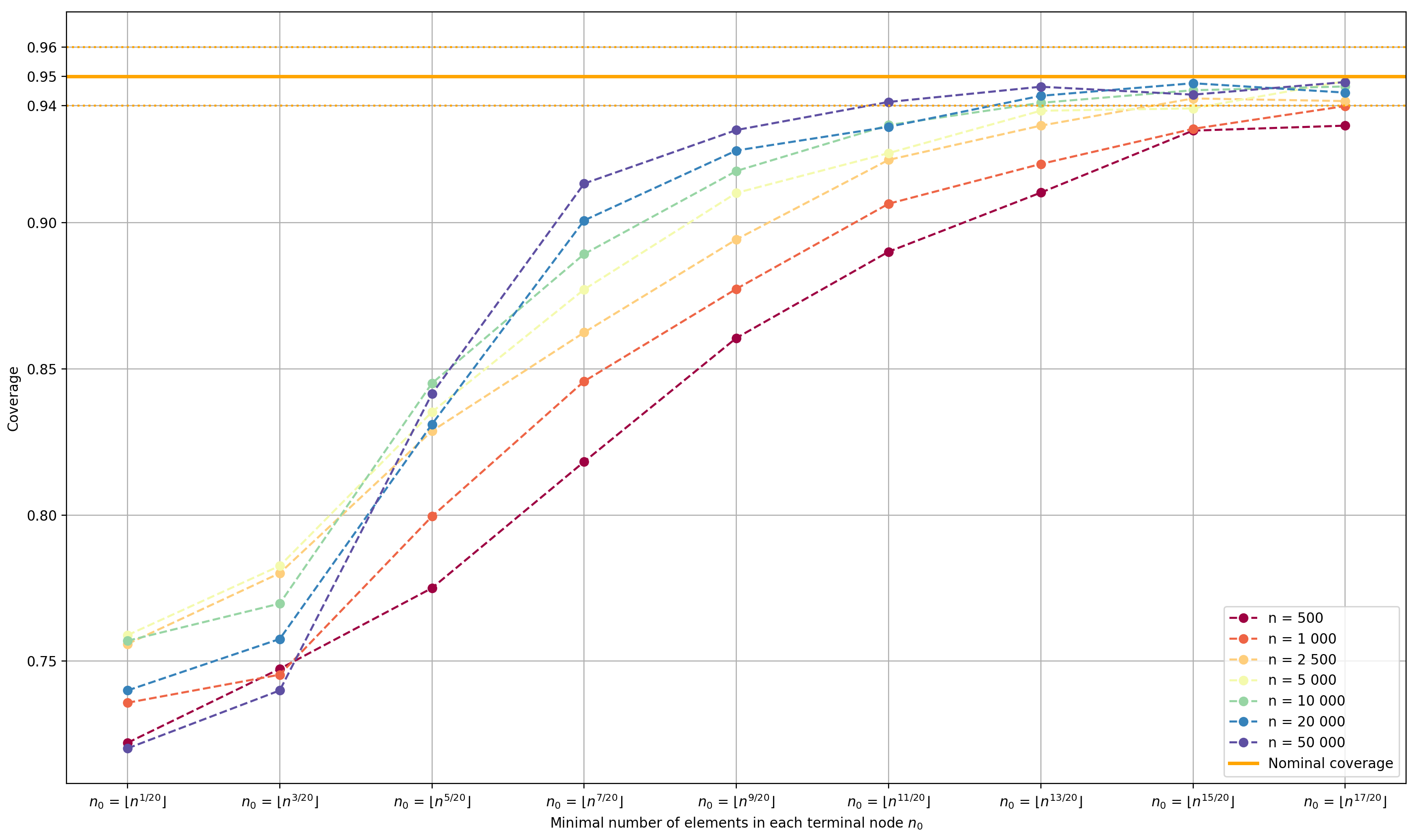
We have also investigated the performance of the variance estimator given by (24) in the case of RF with subsampling, in terms of relative bias and coverage of normal-based confidence intervals. We generated a population of size according to Model 5. The sample size was set to and . Here, we present the results for but other values of led to similar results and are not shown here. As we suspected that the number of observations in each terminal node, may have an impact on the behavior of , we used different values for : for . The choice was advocated by McConville and Toth, 2019. Figure 2 shows the Monte Carlo percent relative bias of for different values of and . Figure 3 shows the Monte Carlo coverage rate of the confidence interval, for different values of and .
From Figure 2, we note that was severely biased for small values of . For a given value of , we note that the bias decreased as increased and for a given value of , the bias decreased as increased. The bias was likely due to the fact that the predicted values in a terminal node are defined as the weighted mean of the sample observations within the same terminal node. As a result, the resulting estimator may suffer from small sample bias for small values of From Figure 3, we note that the confidence intervals performed poorly for small values of , which can be explained by the fact that the variance estimator lead to substantial underestimation of the true variance in these scenarios. For , the confidence intervals performed relatively well with coverage rates close to the nominal rate.

6.3 Choice of hyper-parameters
To get a better understanding of how the choice of hyper-parameters impacts the behavior of model-assisted estimators based on RF, we conducted additional scenarios. We first identified the following important hyper-parameters involved in the RF algorithm of Breiman, 2001:
- i)
The minimal number of observations, in each terminal node;
- ii)
The number of trees in the forest ;
- iii)
The number of variables considered for the search of the best split in the optimization criterion (16);
- iv)
The resampling mechanism.
The additional scenarios were conducted using a finite population of size consisting of the survey variables and described in Section 6.1. Recall that the working model for the survey variables included the predictors -, whereas it included the predictors for the variable (see Table 1).
From the population, we generated samples, of size according to simple random sampling without replacement. Figure 4 and Figure 5 show, respectively, the relative efficiency of the model-assisted estimators based on RF, corresponding to and , respectively, for several values of . Figure 4 suggests that was much more efficient than the Horvitz-Thompson estimator for small values of and that the value of RE approached 100 as increased. This result can be explained by the fact that small values of led to homogeneous terminal nodes, which in turn led to small residuals . For the survey variable , we note from Figure 5 that the value of did not seem to affect the efficiency of the corresponding model-assisted estimator.


Figure 6 display the relative efficiency for several values of the number of trees in the forest for the survey variable . As expected, a small value of causes the estimator to loose some efficiency. Figure 6 suggests that led to good results and that the efficiency of was not much affected by the number of trees for . Nevertheless, it is advisable to choose a large value of if the computational capacity permits. The results for the survey variable were very similar and so we omit them.

In most software packages, the default number of variables considered for the splitting process is in case of regression. In our simulations, this choice led to satisfactory results in most scenarios. Figure 7 shows the relative efficiency of for the survey variable and for several values of . Since the working model for contained explanatory variables, the default value was equal to 10. Although the value was not the best choice for optimal performances, it led efficient model-assisted estimators. Furthermore, the relative efficiency did not vary much for values larger than 30.

Turning to the resampling mechanism, a common choice is to use bootstrap (with replacement), for which some of the results presented in the paper do not apply. However, as noted by several authors (see e.g. Scornet et al., 2015, Wager, 2014 and the references therein) and as shown in our simulations, selecting the points without replacement rather than with replacement does not seem to affect the performance of the resulting model-assisted estimators in most cases.
6.4 Real data application
In this section, we apply the proposed methods using data collected by Médiamétrie, the company that measures the media audience in France. In this application, we focus on radio audiences. Each year, Médiamétrie conducts a survey aiming at gathering detailed information about French individuals 13 years of age and over, including socio-demographic variables and radio listening habits. We used the radio audience data that consisted of individuals. As a survey variable, we considered the binary variable such that if an individual in the th individual listens to the radio of interest on a daily basis, and otherwise. For confidentiality reasons, we omit the name of the radio broadcaster. We aimed at estimating the proportion of French individuals who listen to the radio of interest on a daily basis, both at the overall population level and for several domains of interest. For each individual on the data set, we had access to socio-demographic variables (e.g., number of individuals in the household, age of each member of the household, gender, internet habits, occupation, etc.) and their listening habits of other radios. For each individual, we also knew whether or not the individual listens to any of these 21 radios, for each interval of minutes on a typical day. This led to a data set with variables, among which were binary.
From the data set, we selected a single sample of size according to a stratified sampling design with 5 strata, each stratum corresponding to a French region: North-East, North-West, Île-de-France, South-east and South-West. The strata sample sizes were determined according to proportional allocation. We considered the following domains of interest: the sub-population of individuals who connects to the internet everyday, almost every day, once or twice per week, once to three times per month, very rarely, never, the sub-population of individuals with/without children, the sub-populations of individuals living in cities of size (less than between and between and between and and larger than ) and the sub-population of individuals of size 1, 2, 3, 4, 5 and larger than 5.
We computed the following estimates both at the overall level and at the domain level: (i) The Horvitz-Thompson estimator; (ii) the GREG estimator and (iii) the model-assisted estimator based on RF with hyper-parameters , and . The working models used for the GREG estimator and the model-assisted RF estimator included explanatory variables. In each scenario, we also computed a 95% confidence interval for the proportion in the population of individuals who listen to the radio of interest. Finally, we computed the ratio of the estimated variances, using the estimated variance of the Horvitz-Thompson estimator, as the reference. Note that the "true value" was known for each domain of interest. The results are given in Table 4; for readability purpose, the results are expressed in percentage.
From Table 4, we note that the Horvitz-Thompson estimator performed relatively well in most scenarios. Because of the large number of predictors, the GREG estimator suffered from significant small sample bias. For instance, the estimate based on the GREG estimate at the overall level was equal to 27.7%, far from the true value of about 13.5%. In terms of point estimation, the model-assisted estimator based on RF led to very similar results than those obtained with the Horvitz-Thompson estimator. However, RF led to substantial improvement in terms of estimated variance. Indeed, out of the 22 domains, the value of RV(RF) was smaller than 0.65 for 20 domains. The results suggest that, unlike the GREG estimator, the model-assisted estimator based on RF was not affected by the large number of explanatory variables in the working model. The median length of the confidence intervals was equal to 5.4% for the Horvitz-Thompson estimator, 4.2% for the RF estimator and 3.8% for the GREG estimator.
| Domain | True value | HT | RF | GREG | RV (RF) | RV (GREG) | CI HT | CI RF | CI GREG |
|---|---|---|---|---|---|---|---|---|---|
| Overall | 13.5 | 13.7 | 13.6 | 27.7 | 64.6 | 48.5 | [12.7; 14.7] | [12.8; 14.4] | [27.0; 28.3] |
| Freq: Every day | 14.6 | 14.6 | 14.4 | 28.1 | 61.3 | 44.0 | [13.5; 15.8] | [13.5; 15.3] | [27.3; 28.9] |
| Freq: Almost every day | 14.0 | 15.5 | 14.9 | 31.8 | 62.0 | 52.7 | [11.1; 19.8] | [11.4; 18.3] | [28.6; 35.0] |
| Freq: 1-2 / week | 8.7 | 10.5 | 11.2 | 55.1 | 67.0 | 62.9 | [6.1; 14.9] | [7.6; 14.7] | [51.6; 58.5] |
| Freq: 1-3 / month | 11.3 | 16.1 | 12.8 | 3.8 | 47.6 | 28.1 | [5.8; 26.4] | [5.6; 19.9] | [-1.5; 9.3] |
| Freq: Very rarely | 6.7 | 7.6 | 10.0 | 29.6 | 60.5 | 57.7 | [1.4; 13.8] | [5.2; 14.8] | [24.9; 34.3] |
| Freq: Never | 8.4 | 2.5 | 8.1 | -66.1 | 103 | 125 | [-2.0; 7.0] | [3.4; 12.7] | [-71.2; -61.1] |
| Children: Yes | 11.1 | 11.5 | 11.4 | 33.0 | 57.2 | 40.9 | [9.7; 13.3] | [10.0; 12.7] | [31.9; 34.2] |
| Children: No | 14.4 | 14.5 | 14.5 | 25.7 | 62.3 | 47.4 | [13.3; 15.7] | [13.5; 15.4] | [24.8; 26.5] |
| Inhabitants: Country | 12.7 | 12.8 | 12.6 | 45.4 | 58.9 | 42.6 | [10.5; 15.1] | [10.8; 14.3] | [44.0; 46.9] |
| Inhabitants: <20K | 12.9 | 12.7 | 12.1 | 35.2 | 52.6 | 37.2 | [10.1; 15.3] | [10.2; 14.0] | [33.6; 36.8] |
| Inhabitants: 20-50K | 12.5 | 10.8 | 11.0 | 36.9 | 62.2 | 52.4 | [6.7; 14.9] | [7.8; 14.3] | [33.9; 39.8] |
| Inhabitants: 50-100K | 12.3 | 11.5 | 12.2 | 25.9 | 58.6 | 47.7 | [8.8; 14.2] | [10.1; 14.3] | [24.0; 27.8] |
| Inhabitants: 100-200K | 15.5 | 18.0 | 17.9 | 5.8 | 53.4 | 38.5 | [14.0; 22.0] | [15.0; 20.8] | [3.3; 8.2] |
| Inhabitants: >200K | 14.2 | 14.0 | 14.0 | 27.3 | 60.4 | 46.1 | [12.1; 16.0] | [12.5; 15.6] | [26.0; 28.7] |
| Inhabitants: Paris | 14.3 | 16.3 | 16.0 | 0.6 | 60.7 | 45.3 | [13.0; 19.6] | [13.4; 18.6] | [-1.5; 2.8] |
| N Household: 1 | 13.9 | 13.1 | 13.5 | 8.2 | 58.5 | 44.8 | [11.1; 15.1] | [12.0; 15.1] | [6.8; 9.5] |
| N Household: 2 | 16.3 | 15.9 | 16.1 | 27.3 | 58.1 | 45.7 | [14.0; 17.8] | [14.6; 17.5] | [26.1; 28.6] |
| N Household: 3 | 11.7 | 14.2 | 13.4 | 33.9 | 55.3 | 37.3 | [11.4; 15.4] | [11.5; 16.9] | [32.3; 35.6] |
| N Household: 4 | 11.3 | 12.7 | 11.8 | 50.3 | 56.5 | 41.0 | [10.2; 15.2] | [9.9; 13.7] | [48.7; 51.9] |
| N Household: 5 | 9.7 | 8.2 | 9,1 | 28.4 | 63.1 | 46.2 | [4.9; 11.6] | [6.5; 11.8] | [26.1; 30.6] |
| N Household: >5 | 6.3 | 5.0 | 3.9 | 50.9 | 53.8 | 26.8 | [0.0; 9.5] | [0.0; 7.2] | [48.5; 53.2] |
7 Final remarks
In this paper, we have introduced a new class of model-assisted estimators based on random forests and derived corresponding variance estimators. We have established the theoretical properties of point and variance estimators obtained through a RF algorithm based on subsampling. The results of an empirical study suggest that the proposed estimators perform well in a wide variety of settings, unlike the GREG and CART estimators. In practice, this robustness property is especially attractive when the data and the underlying relationships are complex. The application on radio audience data recorded by the French company Médiamétrie showed that the RF proposed estimator performed well in this high-dimension setting. We have also described a model calibration procedure for handling multiple survey variables, yet producing a single set of weights, which is attractive from a data user’s perspective.
In practice, virtually all survey face the problem of missing values. Survey statisticians distinguish unit nonresponse (when no information is collected on a sampled unit) from item nonresponse (when the absence of information is limited to some variables only). The treatment of unit nonresponse starts with postulating a nonresponse model describing the relationship between the response indicators (equal to 1 for respondents and 0 for nonrespondents) and a vector of explanatory variables. The treatment of item nonresponse starts with postulating an imputation model describing the relationship between the variable requiring imputation and a set of explanatory variables. In both unit and item nonresponse, determining a suitable model is crucial. Therefore, regression trees and RF may prove useful for obtaining accurate estimated response propensities and predicted values. To the best of our knowledge, a theoretical treatment of regression trees and RF in the context of either unit nonresponse or item nonresponse in a finite population setting is lacking. These topics are currently under investigation.
Traditionally, survey samples are collected by probability sampling procedures and inferences are conducted with respect to the customary design-based framework. In recent years, there has been a shift of paradigm that can be explained by three main factors: (i) the dramatic decrease of response rates; (ii) the rapid increase in data collection costs; and (iii) the proliferation of nonprobabilistic data sources (e.g., administrative files, web survey panels, social media data, satellite information, etc.). To meet these new challenges, survey statisticians face increasing pressure to utilize these convenient but often uncontrolled data sources. While such sources provide timely data for a large number of variables and population elements, they often fail to represent the target population of interest because of inherent selection biases. The integration of data from a nonprobability source to data from a probability survey is a topic that is currently being scrutinized by National Statistical Offices. An approach to data integration is statistical matching or mass imputation. Again, regression trees and RF algorithms may be useful techniques in the context of integration of survey data. This topic is currently under investigation.
In a high-dimensional setting, RF may be used to selecting the most predictive predictors, which in turn may be used in the construction of model-assisted estimators of population totals/means. In this context, issues such as variable selection bias (Strobl et al., 2007) in a finite population setting need to be investigated. This will be treated elsewhere.
Appendix
Proof of Proposition 2.1 Since
| (30) |
involves positive quantities only, the weights are nonnegative. Since for all and for all the weight can be bounded as follows:
where does not depend on nor on or . To show ii), fix . The result follows by noting that exactly times.
Proof of Proposition 3.3 Consider the partitions build at the sample level For a given the partition is composed by disjointed regions as follows and for each consider the dimensional vector where if belongs to the region and zero otherwise for all . Since is a partition, then will belong to only one region and so, the vector will contain only one non zero component. We have and can be written as where (see also the supplementary materiel for more details). Now,
For each consider the dimensional vector whose elements are all equal to one, we have then for all so
References
- Arnould et al., (2020) Arnould, L., Boyer, C., and Scornet, E. (2020). Analyzing the tree-layer structure of deep forests. arXiv preprint arXiv:2010.15690.
- Bergstra et al., (2011) Bergstra, J., Bardenet, R., Bengio, Y., and Kégl, B. (2011). Algorithms for hyper-parameter optimization. Advances in neural information processing systems, 24:2546–2554.
- Biau, (2012) Biau, G. (2012). Analysis of a random forests model. Journal of Machine Learning Research, 13(Apr):1063–1095.
- Biau and Devroye, (2014) Biau, G. and Devroye, L. (2014). Cecllular tree classifiers. In International Conference on Algorithmic Learning Theory. Springer.
- Biau et al., (2008) Biau, G., Devroye, L., and Lugosi, G. (2008). Consistency of random forests and other averaging classifiers. Journal of Machine Learning Research, 9(Sep):2015–2033.
- Biau and Scornet, (2016) Biau, G. and Scornet, E. (2016). A random forest guided tour. Test, 25(2):197–227.
- Boistard et al., (2012) Boistard, H., Lopuhaä, H. P., and Ruiz-Gazen, A. (2012). Approximation of rejective sampling inclusion probabilities and application to high order correlations. Electron. J. Stat., 6:1967–1983.
- Breidt et al., (2005) Breidt, F., Claeskens, G., and Opsomer, J. (2005). Model-assisted estimation for complex surveys using penalized splines. Biometrika, 92:831–846.
- Breidt and Opsomer, (2000) Breidt, F.-J. and Opsomer, J.-D. (2000). Local polynomial regression estimators in survey sampling. The Annals of Statistics, 28(4):1023–1053.
- Breidt and Opsomer, (2017) Breidt, F. J. and Opsomer, J. D. (2017). Model-assisted survey estimation with modern prediction techniques. Statistical Science, 32(2):190–205.
- Breiman, (2001) Breiman, L. (2001). Random forests. Machine learning, 45(1):5–32.
- Breiman et al., (1984) Breiman, L., Friedman, J., Olshen, R., and Stone, C. (1984). Classification and Regression Trees. Chapman & Hall/CRC, Boca Raton.
- Buskirk and Kolenikov, (2015) Buskirk, T. D. and Kolenikov, S. (2015). Finding respondents in the forest: A comparison of logistic regression and random forest models for response propensity weighting and stratification. Survey Methods: Insights from the Field, pages 1–17.
- Cardot et al., (2010) Cardot, H., Chaouch, M., Goga, C., and Labruère, C. (2010). Properties of design-based functional principal components analysis. J. of Statistical Planning and Inference, 140:75–91.
- Cardot et al., (2013) Cardot, H., Goga, C., and Lardin, P. (2013). Uniform convergence and asymptotic confidence bands for model-assisted estimators of the mean of sampled functional data. Electronic Journal of Statistics, 7:562–596.
- Cardot et al., (2014) Cardot, H., Goga, C., and Lardin, P. (2014). Variance estimation and asymptotic confidence bands for the mean estimator of sampled functional data with high entropy unequal probability sampling designs. Scandinavian J. of Statistics, 41:516–534.
- Chipman et al., (1998) Chipman, H. A., George, E. I., and McCulloch, R. E. (1998). Bayesian CART model search. Journal of the American Statistical Association, 93(443):935–948.
- De Moliner and Goga, (2018) De Moliner, A. and Goga, C. (2018). Sample-based estimation of mean electricity consumption curves for small domains. Survey Methodology, 44(2):193–214.
- Deville and Särndal, (1992) Deville, J.-C. and Särndal, C.-E. (1992). Calibration estimators in survey sampling. Journal of the American Statistical Association, 87:376–382.
- Devroye et al., (1996) Devroye, L., Gyorfi, L., and Lugosi, G. (1996). A Probabilistic Theory of Pattern Recognition. Springer, New York.
- Díaz-Uriarte and de Andrés, (2006) Díaz-Uriarte, R. and de Andrés, S. (2006). Gene selection and classification of microarray data using random forest. BMC Bioinformatics, 7(1):3.
- Firth and Bennett, (1998) Firth, D. and Bennett, K. (1998). Robust models in probability sampling. Journal of the Royal Statistical Society: Series B (Statistical Methodology), 60(1):3–21.
- Fraiwan et al., (2012) Fraiwan, L., Lweesy, K., Khasawneh, N., Wenz, H., and Dickhaus, H. (2012). Automated sleep stage identification system based on time–frequency analysis of a single EEG channel and random forest classifier. Computer Methods and Programs in Biomedicine, 108(1):10–19.
- Friedman, (2001) Friedman, J. (2001). Greedy function approximation: A gradient boosting machine. The Annals of Statistics, 29(5):1189–1232.
- Fuller, (2009) Fuller, W.-A. (2009). Sampling Statistics. John Wiley & Sons.
- Genuer, (2012) Genuer, R. (2012). Variance reduction in purely random forests. Journal of Nonparametric Statistics, 24(3):543–562.
- Geurts et al., (2006) Geurts, P., Ernst, D., and Wehenkel, L. (2006). Extremely randomized trees. Machine learning, 63(1):3–42.
- Goga, (2005) Goga, C. (2005). Réduction de la variance dans les sondages en présence d’information auxiliaire: une approche non paramétrique par splines de régression. Canad. J. Statist., 33(2):163–180.
- Goga and Ruiz-Gazen, (2014) Goga, C. and Ruiz-Gazen, A. (2014). Efficient estimation of non-linear finite population parameters by using non-parametrics. Journal of the Royal Statistical Society, B, 76:113–140.
- Grimm et al., (2008) Grimm, R., Behrens, T., Märker, M., and Elsenbeer, H. (2008). Soil organic carbon concentrations and stocks on barro colorado island — digital soil mapping using random forests analysis. Geoderma, 146(1-2):102–113.
- Hamza and Larocque, (2005) Hamza, M. and Larocque, D. (2005). An empirical comparison of ensemble methods based on classification trees. Journal of Statistical Computation and Simulation, 75(8):629–643.
- Han et al., (2018) Han, T., Jiang, D., Zhao, Q., Wang, L., and Yin, K. (2018). Comparison of random forest, artificial neural networks and support vector machine for intelligent diagnosis of rotating machinery. Transactions of the Institute of Measurement and Control, 40(8):2681–2693.
- Hastie et al., (2011) Hastie, T., Tibshirani, R., and Friedman, J. (2011). The Elements of Statistical Learning: Data Mining, Inference and Prediction. Springer, New York.
- Isaki and Fuller, (1982) Isaki, C.-T. and Fuller, W.-A. (1982). Survey design under the regression superpopulation model. J. Amer. Statist. Assoc., 77:49–61.
- James et al., (2015) James, G., Witten, D., Hastie, T., and Tibshirani, R. (2015). An Introduction to Statistical Learning with Applications in R. Springer Texts in Statistics.
- Kane et al., (2014) Kane, M., Price, N., Scotch, M., and Rabinowitz, P. (2014). Comparison of arima and random forest time series models for prediction of avian influenza h5n1 outbreaks. BMC Bioinformatics, 15(1).
- Kern et al., (2019) Kern, C., Klausch, T., and Kreuter, F. (2019). Tree-based machine learning methods for survey research. In Survey Research Methods, volume 13, pages 73–93.
- Lehtonen and Veijanen, (1998) Lehtonen, R. and Veijanen, A. (1998). Logistic generalized regression estimators. Survey Methodology, 24:51–56.
- McConville and Breidt, (2013) McConville, K. and Breidt, F. J. (2013). Survey design asymptotics for the model-assisted penalised spline regression estimator. Journal of Nonparametric Regression, 25(3):745–763.
- McConville and Toth, (2019) McConville, K. and Toth, D. (2019). Automated selection of post-strata using a model-assisted regression tree estimator. Scandinavian Journal of Statistics, 46(2):389–413.
- Montanari and Ranalli, (2009) Montanari, G. and Ranalli, M. G. (2009). Multiple and ridge model calibration for sample surveys. unpublished.
- Montanari and Ranalli, (2005) Montanari, G. E. and Ranalli, M. G. (2005). Nonparametric model calibration in survey sampling. J. Amer. Statist. Assoc., 100:1429–1442.
- Najafabadi et al., (2015) Najafabadi, M. M., Villanustre, F., Khoshgoftaar, T. M., Seliya, N., Wald, R., and Muharemagic, E. (2015). Deep learning applications and challenges in big data analytics. Journal of Big Data, 2(1):1.
- Opsomer et al., (2007) Opsomer, J. D., Breidt, F. J., Moisen, G., and Kauermann, G. (2007). Model-assisted estimation of forest resources with generalized additive models. Journal of the American Statistical Association, 102(478):400–409.
- Qi, (2012) Qi, Y. (2012). Random forests for bioinformatics, pages 307–323. Springer.
- Robinson and Särndal, (1983) Robinson, P. M. and Särndal, C.-E. (1983). Asymptotic properties of the generalized regression estimator in probability sampling. Sankhyā Ser. B, 45(2):240–248.
- Rogez et al., (2008) Rogez, G., Rihan, J., Ramalingam, C., Orrite, C., and Torr, P. (2008). Randomized trees for human pose detection. In Computer Vision and Pattern Recognition, CVPR, IEEE Conference on., pages 1–8.
- Santacatterina and Bottai, (2018) Santacatterina, M. and Bottai, M. (2018). Optimal probability weights for inference with constrained precision. Journal of the American Statistical Association, 113(523):983–991.
- Särndal, (1980) Särndal, C.-E. (1980). On the -inverse weighting best linear unbiased weighting in probability sampling. Biometrika, 67:639–650.
- Särndal et al., (1992) Särndal, C.-E., Swensson, B., and Wretman, J. (1992). Model assisted survey sampling. Springer Series in Statistics. Springer-Verlag, New York.
- Särndal and Wright, (1984) Särndal, C.-E. and Wright, R. (1984). Cosmetic form of estimators in survey sampling. Scandinavian J. of Statistics, 11:146–156.
- (52) Scornet, E. (2016a). On the asymptotics of random forests. Journal of Multivariate Analysis, 146:72–83.
- (53) Scornet, E. (2016b). Random forests and kernel methods. IEEE Transactions on Information Theory, 62:1485–1500.
- Scornet, (2017) Scornet, E. (2017). Tuning parameters in random forests. ESAIM: Proceedings and Surveys, 60:144–162.
- Scornet et al., (2015) Scornet, E., Biau, G., and Vert, J.-P. (2015). Consistency of random forests. The Annals of Statistics, 43(4):1716–1741.
- Stekhoven and Buhlmann, (2011) Stekhoven, D. J. and Buhlmann, P. (2011). MissForest–non-parametric missing value imputation for mixed-type data. Bioinformatics, 28(1):112–118.
- Strobl et al., (2007) Strobl, C., Boulesteix, A., Zeileis, A., and Hothorn, T. (2007). Bias in random forest variable importance measures: Illustrations, sources and a solution. BMC BioInformatics, 25(8).
- Tipton et al., (2013) Tipton, J., Opsomer, J., and Moisen, G. (2013). Properties of endogenous post-stratified estimation using remote sensing data. Remote sensing of environment, 139:130–137.
- Toth and Eltinge, (2011) Toth, D. and Eltinge, J. L. (2011). Building consistent regression trees from complex sample data. Journal of the American Statistical Association, 106(496):1626–1636.
- Wager, (2014) Wager, S. (2014). Asymptotic theory for random forests. arXiv preprint arXiv:1405.0352.
- Wang and Wang, (2011) Wang, L. and Wang, S. (2011). Nonparametric additive modelassisted estimation for survey data. Journal of Multivariate Analysis, 102:1126–1140.
- Wright and Ziegler, (2015) Wright, M. and Ziegler, A. (2015). ranger: A fast implementation of random forests for high dimensional data in c++ and r. arXiv preprint arXiv:1508.04409.
- Wu and Sitter, (2001) Wu, C. and Sitter, R. R. (2001). A model-calibration approach to using complete auxiliary information from survey data. Journal of the American Statistical Association, 96:185–193.