Testing the Agreement of Trees with Internal Labels

A close relative of the agreement problem is the compatibility problem. The input to the compatibility problem is a profile $\mathcal{P}=\{\mathcal{T}_{1},\mathcal{T}_{2},\ldots,\mathcal{T}_{k}\}$ of rooted phylogenetic trees with partially overlapping taxon sets. The question is whether there exists a tree $\mathcal{T}$ whose taxon set is the union of the taxon sets of the input trees such that each input tree $\mathcal{T}_{i}$ can be obtained from the restriction of $\mathcal{T}$ to the taxon set of $\mathcal{T}_{i}$ through edge contractions. If such a tree $\mathcal{T}$ exists, we refer to $\mathcal{T}$ as a compatible tree for $\mathcal{P}$ and say that $\mathcal{P}$ is compatible; otherwise, $\mathcal{P}$ is incompatible. Compatibility is a less stringent requirement than agreement; therefore, any profile that agrees is compatible, but the converse is not true. The compatibility problem for phylogenies (i.e., trees without internal labels), is solvable in $\mathcal{O}(M_{\mathcal{P}}\log^{2}M_{\mathcal{P}})$ time, where $M_{\mathcal{P}}$ is the total number of nodes and edges in the trees of $\mathcal{P}$ [9]. Note that $M_{\mathcal{P}}=\mathcal{O}(nk)$.

Compatibility and agreement reflect two distinct approaches to dealing with multifurcations; i.e., non-binary nodes, also known as polytomies. Suppose that node $v$ is a multifurcation in some input tree of $\mathcal{P}$ and that $\ell_{1}$, $\ell_{2}$, and $\ell_{3}$ are taxa in three distinct subtrees of $v$. In an agreement tree for $\mathcal{P}$, these three taxa must be in distinct subtrees of some node in the agreement tree. In contrast, a compatible tree for $\mathcal{P}$ may contain no such node, since a compatible tree is allowed to “refine” the multifurcation at $v$ — that is, group two out of $\ell_{1}$, $\ell_{2}$, and $\ell_{3}$ separately from the third. Thus, compatibility treats multifurcations as “soft” facts; agreement treats them as “hard” facts [15]. Both viewpoints can be valid, depending on the circumstances.

The agreement and compatibility problems are fundamental special cases of the supertree problem, the problem of synthesizing a collection of phylogenetic trees with partially overlapping taxon sets into a single supertree that represents the information in the input trees [4, 2, 18, 24]. The original supertree methods were limited to input trees where only the leaves are labeled, but there has been increasing interest in incorporating internally labeled trees in supertree analysis, motivated by the desire to incorporate taxonomies in these analyses. Taxonomies group organisms according to a system of taxonomic rank (e.g., family, genus, and species); two examples are the NCBI taxonomy [21] and the Angiosperm taxonomy [23]. Taxonomies provide structure and completeness that can be hard to obtain otherwise [17, 12, 19], offering a way to circumvent one of the obstacles to building comprehensive phylogenies: the limited taxonomic overlap among different phylogenetic studies [20].

Although internally labeled trees, and taxonomies in particular, are not, strictly speaking, phylogenies, they have many of the same mathematical properties as phylogenies. Both phylogenies and internally labeled trees are $X$-trees (also called semi-labeled trees) [5, 22]. Algorithmic results for compatibility and agreement of internally labeled trees are scarce, compared to what is available for ordinary phylogenies. To our knowledge, the first algorithm for testing compatibility of internally labeled trees is in [7] (see also [3]). The fastest known algorithm for the problem runs in $\mathcal{O}(M_{\mathcal{P}}\log^{2}M_{\mathcal{P}})$ time [8]. We are unaware of any previous algorithmic results for the agreement problem for internally labeled trees.

All algorithms for compatibility and agreement that we know of are indebted to Aho et al.’s Build algorithm [1]. The time bounds for agreement algorithms are higher than those of compatibility algorithms, due to the need for agreement trees to respect the multifurcations in the input trees. To handle agreement, Build has to be modified so that certain sets of the partition of the taxa it generates are re-merged to reflect the multifurcations in the input trees, adding considerable overhead [16, 10] (similar issues are faced when testing consistency of triples and fans [14]). This issue becomes more complex for internally labeled trees, in part because internal nodes with the same label, but in different trees, may jointly imply multifurcations, even if all input trees are binary.

Section 2 provides a formal definition of the agreement problem for internally labeled trees. Section 3 studies the decomposability properties of profiles that agree. These properties allow us to reduce an agreement problem on a profile into independent agreement problems on subprofiles, leading to the agreement algorithm presented in Section 4. Section 5 contains some final remarks. All proofs are in the Appendix.

Let $G$ be a graph. $V(G)$ and $E(G)$ denote the node and edge sets of $G$. Let $U$ be a subset of $V(G)$. Then the subgraph of $G$ induced by $U$ is the graph whose vertex set is $U$ and whose edge set consists of all of the edges in $E(G)$ that have both endpoints in $U$.

A tree is an acyclic connected graph. All trees here are assumed to be rooted. For a tree $T$, $r(T)$ denotes the root of $T$. Suppose $u,v\in V(T)$. Then, $u$ is an ancestor of $v$ in $T$, denoted $u\leq_{T}v$, if $u$ lies on the path from $v$ to $r(T)$ in $T$. If $u\leq_{T}v$, then $v$ is a descendant of $u$. Node $u$ is a proper ancestor of $v$, denoted $u<_{T}v$, if $u\leq_{T}v$ and $u\neq v$. If $\{u,v\}\in E(T)$ and $u\leq_{T}v$, then $u$ is the parent of $v$ and $v$ is a child of $u$. For each $x\in V(T)$, we use ${\rm parent}_{T}(x)$, and ${\mathrm{Ch}}_{T}(x)$, $T(x)$ to denote the parent of $x$, the children of $x$, and the subtree of $T$ rooted at $x$, respectively. We extend the child notation to subsets of $V(T)$ in the natural way: for $U\subseteq V(T)$, ${\mathrm{Ch}}_{T}(U)=\bigcup_{u\in U}{\mathrm{Ch}}_{T}(u)$. Thus, if $U=\emptyset$, then ${\mathrm{Ch}}_{T}(U)=\emptyset$.

Let $T$ be a tree and suppose $U\subseteq V(T)$. The lowest common ancestor of $U$ in $T$, denoted $\mathrm{LCA}_{T}(U)$, is the unique smallest upper bound of $U$ under $\leq_{T}$.

Throughout the paper, $X$ denotes a set of labels (that is, taxa, which may be, e.g., species or families of species). An $X$-tree is a pair $\mathcal{T}=(T,\phi)$ where $T$ is a tree and $\phi$ is a mapping from $X$ to $V(T)$ such that, for every node $v\in V(T)$ of degree at most two, $v\in\phi(X)$. $X$ is the label set of $\mathcal{T}$ and $\phi$ is the labeling function of $\mathcal{T}$. For every node $v\in V(T)$, $\phi^{-1}(v)$ denotes the (possibly empty) subset of $X$ whose elements map into $v$; these elements as the labels of $v$. If $\phi^{-1}(v)\neq\emptyset$, then $v$ is labeled; otherwise, $v$ is unlabeled.

By definition, every leaf in an $X$-tree is labeled, and any node, including the root, that has a single child must be labeled. Nodes with two or more children may be labeled or unlabeled. An $X$-tree $\mathcal{T}=(T,\phi)$ is singly labeled if every node in $T$ has at most one label; $\mathcal{T}$ is fully labeled if every node in $T$ is labeled.

$X$-trees, also known as semi-labeled trees, generalize ordinary phylogenetic trees (also known as phylogenetic $X$-trees [22]). An ordinary phylogenetic tree is a semi-labeled tree $\mathcal{T}=(T,\phi)$ where $r(T)$ has degree at least two and $\phi$ is a bijection from $L(\mathcal{T})$ into leaf set of $T$ (thus, internal nodes are not labeled).

Let $\mathcal{T}=(T,\phi)$ be an $X$-tree. For each $u\in V(T)$, $X(u)$ denotes the set of all labels in the subtree of $T$ rooted at $u$; that is, $X(u)=\bigcup_{v:u\leq_{T}v}\phi^{-1}(v)$. $X(u)$ is called a cluster of $T$. ${\mathrm{Cl}}(\mathcal{T})$ denotes the set of all clusters of $\mathcal{T}$. We extend the cluster notation to sets of nodes as follows. Let $U$ be a subset of $V(T)$. Then, $X(U)=\bigcup_{v\in U}X(v)$. If $U=\emptyset$, then $X(U)=\emptyset$.

Suppose $Y\subseteq X$ for an $X$-tree $\mathcal{T}=(T,\phi)$. The restriction of $\mathcal{T}$ to $Y$, denoted $\mathcal{T}|Y$, is the semi-labeled tree whose cluster set is ${\mathrm{Cl}}(\mathcal{T}|Y)=\{W\cap Y:W\in{\mathrm{Cl}}(\mathcal{T})\text{ and }W\cap Y\neq\emptyset\}.$ Intuitively, $\mathcal{T}|Y$ is obtained from the minimal rooted subtree of $T$ that connects the nodes in $\phi(Y)$ by suppressing all vertices $v$ such that $v\notin\phi(Y)$ and $v$ has only one child.

Let $\mathcal{T}=(T,\phi)$ be an $X$-tree and $\mathcal{T}^{\prime}=(T^{\prime},\phi^{\prime})$ be an $X^{\prime}$-tree such that $X^{\prime}\subseteq X$. $\mathcal{T}$ agrees with $\mathcal{T}^{\prime}$ if ${\mathrm{Cl}}(\mathcal{T}^{\prime})={\mathrm{Cl}}(\mathcal{T}|X^{\prime})$. It is well known that the clusters of a tree determine the tree, up to isomorphism [22, Theorem 3.5.2]. Thus, $\mathcal{T}$ agrees with $\mathcal{T}^{\prime}$ if $\mathcal{T}^{\prime}$ and $\mathcal{T}|X^{\prime}$ are isomorphic.

Throughout the rest of this paper, $\mathcal{P}$ denotes a set $\{\mathcal{T}_{1},\mathcal{T}_{2},\dots,\mathcal{T}_{k}\}$ such that, for each $i\in[k]$, $\mathcal{T}_{i}=(T_{i},\phi_{i})$ is a phylogenetic $X_{i}$-tree for some set $X_{i}$ (Figure 1a). We refer to $\mathcal{P}$ as a profile, and to the trees in $\mathcal{P}$ as input trees. We write $X_{\mathcal{P}}$ to denote $\bigcup_{i\in[k]}X_{i}$.

A profile $\mathcal{P}$ agrees if there is an $X_{\mathcal{P}}$-tree $\mathcal{T}$ that agrees with each of the trees in $\mathcal{P}$. If $\mathcal{T}$ exists, we refer to $\mathcal{T}$ as an agreement tree for $\mathcal{P}$. See Figure 1b.

Given a subset $Y$ of $X_{\mathcal{P}}$, the restriction of $\mathcal{P}$ to $Y$, denoted $\mathcal{P}|Y$, is the profile defined as $\mathcal{P}|Y=\{\mathcal{T}_{1}|Y\cap X_{1},\mathcal{T}_{2}|Y\cap X_{2},\dots,\mathcal{T}_{k}|Y\cap X_{k}\}.$ The proof of the following lemma is straightforward.

Suppose $\mathcal{P}$ contains trees that are not fully labeled. We can convert $\mathcal{P}$ into an equivalent profile $\mathcal{P}^{\prime}$ of fully-labeled trees as follows. For each $i\in[k]$, let $l_{i}$ be the number of unlabeled nodes in $T_{i}$. Create a set $X^{\prime}$ of $n^{\prime}=\sum_{i\in[k]}l_{i}$ labels such that $X^{\prime}\cap X_{\mathcal{P}}=\emptyset$. For each $i\in[k]$ and each $v\in V(T_{i})$ such that $\phi_{i}^{-1}(v)=\emptyset$, make $\phi_{i}^{-1}(v)=\{\ell\}$, where $\ell$ is a distinct element from $X^{\prime}$. We refer to $\mathcal{P}^{\prime}$ as the profile obtained by adding distinct new labels to $\mathcal{P}$ (see Figure 1a).

From this point forward, we make the following assumption.

By Lemma 2, no generality is lost in assuming that all trees in $\mathcal{P}$ are fully labeled. The assumption that the trees are singularly labeled is inessential; it is only for clarity. Note that, even with the latter assumption, a tree that agrees with $\mathcal{P}$ is not necessarily singularly labeled. Figure 1b illustrates this fact.

By Assumption 1, for each $i\in[k]$, there is a bijection between the labels in $X_{i}$ and the nodes of $V(T_{i})$. For this reason, we will often refer to nodes by their labels. In particular, given a label $\ell\in X_{i}$, we write $X_{i}(\ell)$ to denote $X_{i}(\phi_{i}(\ell))$ (the cluster of $\mathcal{T}_{i}$ at the node labeled $\ell$), ${\mathrm{Ch}}_{T_{i}}(\ell)$ to denote $\phi_{i}({\mathrm{Ch}}_{T_{i}}(\phi_{i}(\ell))$ (the labels of children of $\ell$ in $\mathcal{T}_{i}$), and, for $A\subseteq X_{i}$, ${\mathrm{Ch}}_{T_{i}}(A)$ to denote $\phi_{i}({\mathrm{Ch}}_{T_{i}}(\phi_{i}(A))$.

The following characterization of agreement generalizes a result in [10].

We refer to a function $\phi_{i}$ satisfying conditions (E1)–(E3) of Lemma 4 as a topological embedding of $\mathcal{T}_{i}$ into $\mathcal{T}$. Observe that, by transitivity, condition (E2) implies that, for any $a,b\in X_{i}$, if $a<_{T_{i}}b$, then $\phi_{i}(a)<_{T}\phi_{i}(b)$.

In what follows, $\pi$ denotes a valid position in $\mathcal{P}$. For each $i\in[k]$ such that $\pi_{i}\neq\emptyset$, let $\ell_{i}\in X_{i}$ denote the single label in $\pi_{i}$. Let ${\mathrm{Ch}}_{\mathcal{P}}(\pi)$ denote the set of all children of some label in $\pi$; i.e., ${\mathrm{Ch}}_{\mathcal{P}}(\pi)=\bigcup_{i\in[k]}{\mathrm{Ch}}_{T_{i}}(\pi_{i})$.

Let $\pi$ be a valid position in $\mathcal{P}$. A good decomposition of $\pi$ is a pair $(S,\Pi)$, where $S$ is a subset of the exposed labels in $\bigcup_{i\in\pi_{i}}\pi_{i}$ and $\Pi=\{\pi^{(1)},\pi^{(2)},\dots,\pi^{(d)}\}$ is a collection of valid positions such that

1. (D1)

   $S\cup\bigcup_{j\in[d]}X_{\mathcal{P}}(\pi^{(j)})=X_{\mathcal{P}}(\pi)$ and $S\cap\bigcup_{j\in[d]}X_{\mathcal{P}}(\pi^{(j)})=\emptyset$, and

2. (D2)

   $X_{\mathcal{P}}(\pi^{(p)})\cap X_{\mathcal{P}}(\pi^{(q)})=\emptyset$, for all $p,q\in[d]$ such that $p\neq q$.

Note that we allow $S$ or $\Pi$ to be empty. We refer to the labels in $S$ as semi-universal labels and to the positions in $\Pi$ as successor positions of $\pi$. The next result is central to our agreement algorithm.

To find a good decomposition of a position $\pi$, it is convenient to work with partitions of ${\mathrm{Ch}}_{\mathcal{P}}(\pi)$. (Recall that a partition of a set $Y$ is a collection $\Gamma$ of nonempty subsets of $Y$ such that every element $x\in Y$ is in exactly one set in $\Gamma$.) A good decomposition $(S,\Pi)$, where $\Pi=\{\pi^{(j)}\}_{j\in[d]}$ defines a partition $\Gamma$ of the set ${\mathrm{Ch}}_{\mathcal{P}}(\pi)$ where, for any $a,b\in{\mathrm{Ch}}_{\mathcal{P}}(\pi)$, $a$ and $b$ are in the same set of $\Gamma$ if and only if there exists $j\in[d]$ such that $a,b\in X_{\mathcal{P}}(\pi^{(j)})$. We refer to $\Gamma$ as the partition of ${\mathrm{Ch}}_{\mathcal{P}}(\pi)$ associated with $(S,\Pi)$. Next, we show that, conversely, certain partitions of ${\mathrm{Ch}}_{\mathcal{P}}(\pi)$ define good decompositions of $\pi$.

Set $A\subseteq{\mathrm{Ch}}_{\mathcal{P}}(\pi)$ is nice with respect to a subset $S$ of the exposed labels in $\pi$ if, for each $i\in[k]$ and each label $\ell\in\bigcup_{i\in[k]}\pi_{i}$ such that ${\mathrm{Ch}}_{\mathcal{P}}(\ell)\cap A\neq\emptyset$,

1. (N1)

   if $\ell\in S$ and each $i\in[k]$ such that $\ell\in\pi_{i}$, then $|{\mathrm{Ch}}_{T_{i}}(\ell)\cap A|=1$, and

2. (N2)

   if $\ell\not\in S$, then ${\mathrm{Ch}}_{\mathcal{P}}(\ell)\subseteq X_{\mathcal{P}}(A)$.

Suppose $A$ is a nice set. The position associated with $A$ is the position $\pi^{A}$, where, for each $i\in[k]$, $\pi_{i}^{A}$ is defined as follows. If $\pi_{i}=\emptyset$, then $\pi_{i}^{A}=\emptyset$. Otherwise, let $\ell$ be the single element in $\pi_{i}$. Then,

A partition $\Gamma$ of ${\mathrm{Ch}}_{\mathcal{P}}(\pi)$ is good with respect to $S$ if each set $A\in\Gamma$ is nice with respect to $S$ and, for every two distinct sets $A,B\in\Gamma$, $X_{\mathcal{P}}(\pi^{A})\cap X_{\mathcal{P}}(\pi^{B})=\emptyset$.

We refer to the good partition $(S,\Gamma)$ of ${\mathrm{Ch}}_{\mathcal{P}}(\pi)$ obtained from a good decomposition $(S,\Pi)$ of $\pi$, as described in Lemma 7 (i), as the good partition of ${\mathrm{Ch}}_{\mathcal{P}}(\pi)$ associated with $(S,\Pi)$. Likewise, we refer to the good decomposition $(S,\Pi)$ of $\pi$ obtained from a good partition $(S,\Gamma)$ of ${\mathrm{Ch}}_{\mathcal{P}}(\pi)$, as described in Lemma 7 (ii), as the good decomposition of ${\mathrm{Ch}}_{\mathcal{P}}(\pi)$ associated with $(S,\Gamma)$.

Let $(S,\Gamma),(S^{\prime},\Gamma^{\prime})$ be good partitions of ${\mathrm{Ch}}_{\mathcal{P}}(\pi)$. We say that $(S,\Gamma)$ is finer than $(S^{\prime},\Gamma^{\prime})$, denoted $(S,\Gamma)\sqsubseteq(S^{\prime},\Gamma^{\prime})$, if and only if, $S\supseteq S^{\prime}$ and, for every $A\in\Gamma$, there exists an $A^{\prime}\in\Gamma^{\prime}$ such that $A\subseteq A^{\prime}$. We write $(S,\Gamma)\sqsubset(S^{\prime},\Gamma^{\prime})$ to denote that $(S,\Gamma)\sqsubseteq(S^{\prime},\Gamma^{\prime})$ and $(S,\Gamma)\neq(S^{\prime},\Gamma^{\prime})$. We say that a partition $(S,\Gamma)$ of ${\mathrm{Ch}}_{\mathcal{P}}(\pi)$ is minimal if there does not exist another partition $(S^{\prime},\Gamma^{\prime})$ of ${\mathrm{Ch}}_{\mathcal{P}}(\pi)$ such that $(S^{\prime},\Gamma^{\prime})\sqsubset(S,\Gamma)$.

We refer to the (unique) good decomposition $(S,\Pi)$ associated with the minimal good partition of ${\mathrm{Ch}}_{\mathcal{P}}(\pi)$ as the maximal good decomposition of $\pi$.

GetDecomposition (Algorithm 2) computes a maximal good decomposition of a position $\pi$, relying on an auxiliary graph known as the display graph of the input profile and denoted by $H_{\mathcal{P}}$ [6, 8, 9]. The graph $H_{\mathcal{P}}$ is obtained from the disjoint union of the underlying trees $T_{1},\dots,T_{k}$ of the $\mathcal{P}$ by identifying nodes that have the same label. Multiple edges between the same pair of nodes are replaced by a single edge. See Figure 2.

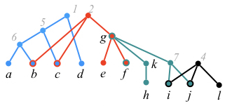
$H_{\mathcal{P}}$ has $O(nk)$ nodes and edges, and can be constructed in $O(nk)$ time. By Assumption 1, there is a bijection between the labels in $X$ and the nodes of $H_{\mathcal{P}}$. Thus, from this point forward, we refer to the nodes of $H_{\mathcal{P}}$ by their labels. For a valid position $\pi$, $H_{\mathcal{P}}(\pi)$ denotes the subgraph of $H_{\mathcal{P}}$ induced by $X(\pi)$. Thus, $H_{\mathcal{P}}(\pi^{\mathrm{init}})=H_{\mathcal{P}}$.

Lines 2–2 of GetDecomposition construct the minimal good partition of ${\mathrm{Ch}}_{\mathcal{P}}(\pi)$. Line 2 initializes $S$ to contain all exposed labels in $\pi$, and sets $K$ to consist of the indices of the trees in $\mathcal{P}$ that contain the labels in $S$. Line 2 initializes $\Gamma$ using $H_{\mathcal{P}}(\pi)$. We say that a label $\ell\in S$ is bad if there exist $i\in K$ and $A\in\Gamma$ such that $\pi_{i}=\{\ell\}$ and $|{\mathrm{Ch}}_{T_{i}}(\ell)\cap A|\geq 2$. Lines 2–2 construct the minimal nice partition $(S,\Gamma)$ of ${\mathrm{Ch}}_{\mathcal{P}}(\pi)$ by deleting bad labels from $S$ and merging sets in $\Gamma$ accordingly. Let $(S^{*},\Gamma^{*})$ denote the minimal good partition of ${\mathrm{Ch}}_{\mathcal{P}}(\pi)$.

By Lemma 9, the pair $(S,\Gamma)$ constructed in lines 2–2 of GetDecomposition is a minimal good partition of ${\mathrm{Ch}}_{\mathcal{P}}(\pi)$. The foreach loop of lines 2–2 simply uses Equation (1) to construct the maximal good decomposition $(S,\Pi)$ of $\pi$ from $(S,\Gamma)$. We thus have the following.

Throughout its execution, BuildAST maintains the display graph $H_{\mathcal{P}}$. Also, for each label $\ell\in X$, it maintains a field $\ell.\mathtt{appear}$ containing every index $i$ such that $\pi_{i}=\{\ell\}$ for some $\pi$ in $Q$. Label $\ell$ is exposed when $|\ell.\mathtt{appear}|=k_{\ell}$, where $k_{\ell}$ denotes the number of input trees containing label $\ell$. For each $\pi$ in BuildAST’s queue, the set ${\mathrm{Ch}}_{\mathcal{P}}(\pi)$ is stored as a sparse array $((i,{\mathrm{Ch}}_{T_{i}}(\pi_{i})):i\in[k]\text{ and }{\mathrm{Ch}}_{T_{i}}(\pi_{i}))\neq\emptyset)$. This enables GetDecomposition to access the parts of ${\mathrm{Ch}}_{\mathcal{P}}(\pi)$ associated with each input tree separately. We use this representation of ${\mathrm{Ch}}_{\mathcal{P}}(\pi)$ to build similar representations of the sets in the partition $\Gamma$ of ${\mathrm{Ch}}_{\mathcal{P}}(\pi)$ produced from $H_{\mathcal{P}}(\pi)\setminus S$ in line 2 of GetDecomposition. For each label $a\in{\mathrm{Ch}}_{\mathcal{P}}(\pi)$, we maintain a mapping that returns, in $O(1)$ time, the set $A\in\Gamma$ containing $a$. During the execution of GetDecomposition’s while loop, sets in $\Gamma$ may be merged, and representations of these merged sets must be produced and the mapping from ${\mathrm{Ch}}_{\mathcal{P}}(\pi)$ to $\Gamma$ must be modified.

In the following results, $d_{i}$ denotes the maximum number of children of a node in tree $T_{i}$, for each $i\in[d]$.

References

- [1] Aho, A., Sagiv, Y., Szymanski, T., Ullman, J.: Inferring a tree from lowest common ancestors with an application to the optimization of relational expressions. SIAM J. Computing 10(3), 405—421 (1981)
- [2] Baum, B.R.: Combining trees as a way of combining data sets for phylogenetic inference, and the desirability of combining gene trees. Taxon 41, 3–10 (1992)
- [3] Berry, V., Semple, C.: Fast computation of supertrees for compatible phylogenies with nested taxa. Systematic Biology 55(2), 270–288 (2006)
- [4] Bininda-Emonds, O.R.P. (ed.): Phylogenetic Supertrees: Combining Information to Reveal the Tree of Life, Series on Computational Biology, vol. 4. Springer, Berlin (2004)
- [5] Bordewich, M., Evans, G., Semple, C.: Extending the limits of supertree methods. Annals of Combinatorics 10, 31–51 (2006)
- [6] Bryant, D., Lagergren, J.: Compatibility of unrooted phylogenetic trees is FPT. Theoretical Computer Science 351, 296–302 (2006)
- [7] Daniel, P., Semple, C.: Supertree algorithms for nested taxa. In: Bininda-Emonds, O.R.P. (ed.) Phylogenetic supertrees: Combining information to reveal the Tree of Life, pp. 151–171. Kluwer, Dordrecht (2004)
- [8] Deng, Y., Fernández-Baca, D.: An efficient algorithm for testing the compatibility of phylogenies with nested taxa. Algorithms for Molecular Biology 12, 7 (2017)
- [9] Deng, Y., Fernández-Baca, D.: Fast compatibility testing for rooted phylogenetic trees. Algorithmica 80(8), 2453–2477 (2018). https://doi.org/10.1007/s00453-017-0330-4, http://rdcu.be/thB1
- [10] Fernández-Baca, D., Guillemot, S., Shutters, B., Vakati, S.: Fixed-parameter algorithms for finding agreement supertrees. SIAM Journal on Computing 44(2), 384–410 (2015)
- [11] Fernández-Baca, D., Liu, L.: Tree compatibility, incomplete directed perfect phylogeny, and dynamic graph connectivity: An experimental study. Algorithms 12(3), 53 (2019)
- [12] Hinchliff, C.E., Smith, S.A., Allman, J.F., Burleigh, J.G., Chaudhary, R., Coghill, L.M., Crandall, K.A., Deng, J., Drew, B.T., Gazis, R., Gude, K., Hibbett, D.S., Katz, L.A., Laughinghouse IV, H.D., McTavish, E.J., Midford, P.E., Owen, C.L., Reed, R.H., Reesk, J.A., Soltis, D.E., Williams, T., Cranston, K.A.: Synthesis of phylogeny and taxonomy into a comprehensive tree of life. Proceedings of the National Academy of Sciences 112(41), 12764–12769 (2015). https://doi.org/10.1073/pnas.1423041112
- [13] Holm, J., de Lichtenberg, K., Thorup, M.: Poly-logarithmic deterministic fully-dynamic algorithms for connectivity, minimum spanning tree, 2-edge, and biconnectivity. J. ACM 48(4), 723–760 (Jul 2001). https://doi.org/10.1145/502090.502095, http://doi.acm.org/10.1145/502090.502095
- [14] Jansson, J., Lingas, A., Rajaby, R., Sung, W.K.: Determining the consistency of resolved triplets and fan triplets. In: International Conference on Research in Computational Molecular Biology. pp. 82–98. Springer (2017)
- [15] Maddison, W.P.: Reconstructing character evolution on polytomous cladograms. Cladistics 5, 365–377 (1989)
- [16] Ng, M., Wormald, N.: Reconstruction of rooted trees from subtrees. Discrete Applied Mathematics 69(1–2), 19–31 (1996)
- [17] Page, R.M.: Taxonomy, supertrees, and the tree of life. In: Bininda-Emonds, O.R.P. (ed.) Phylogenetic supertrees: Combining information to reveal the Tree of Life, pp. 247–265. Kluwer, Dordrecht (2004)
- [18] Ragan, M.A.: Phylogenetic inference based on matrix representation of trees. Molecular Phylogenetics and Evolution 1, 53–58 (1992)
- [19] Redelings, B.D., Holder, M.T.: A supertree pipeline for summarizing phylogenetic and taxonomic information for millions of species. PeerJ 5, e3058 (2017). https://doi.org/10.7717/peerj.3058
- [20] Sanderson, M.J.: Phylogenetic signal in the eukaryotic tree of life. Science 321(5885), 121–123 (2008)
- [21] Sayers et al., E.W.: Database resources of the National Center for Biotechnology Information. Nucleic Acids Research 37(Database issue), D5–D15 (2009)
- [22] Semple, C., Steel, M.: Phylogenetics. Oxford Lecture Series in Mathematics, Oxford University Press, Oxford (2003)
- [23] The Angiosperm Phylogeny Group: An update of the Angiosperm Phylogeny Group classification for the orders and families of flowering plants: APG IV. Botanical Journal of the Linnean Society 181, 1–20 (2016)
- [24] Warnow, T.: Supertree construction: Opportunities and challenges. Tech. Rep. arXiv:1805.03530, ArXiV (May 2018), https://arxiv.org/abs/1805.03530
- [25] Wulff-Nilsen, C.: Faster deterministic fully-dynamic graph connectivity. In: Proceedings of the Twenty-fourth Annual ACM-SIAM Symposium on Discrete Algorithms. pp. 1757–1769. SODA ’13, Society for Industrial and Applied Mathematics, Philadelphia, PA, USA (2013), http://dl.acm.org/citation.cfm?id=2627817.2627943
Appendix 0.A Omitted Proofs
Proof of Lemma 3
Suppose there is a node such that . Note that cannot be a leaf. Let be the children of . One can prove the following.
Fact. For each , there is at most one such that .
Now, choose any . Let be the tree obtained by contracting the edge . That is, is obtained by eliminating edge , deleting , and making . Let , where , if and . Then, the above fact implies that, for each , . That is, is also an agreement tree for . If we repeat this contraction operation until it no longer applies, the final tree will satisfy for each node .
Proof of Lemma 4
We argue that, for each , agrees with if and only if there exists a topological embedding of into .
() Suppose that is a topological embedding from to . We show that , which implies that agrees with .
First, we show that by arguing that, for each , . By definition of LCAs, . Now, suppose that there is a label such that . Let . Then, . On the other hand, , contradicting condition (E2).
Next, we prove that . Suppose, to the contrary, that there is a cluster . Let be the (unique) label such that and for every either or . Since , there must exist at least two labels such that and at least one label such that . Therefore, there is a single node such that , contradicting condition (E3).
() Suppose that agrees with . It is straightforward to show that must satisfy (E1). Thus, we focus on conditions (E2) and (E3).
Suppose condition (E2) does not hold. Then, there exists a label , such that . Since , we must in fact have . But then does not agree with , a contradiction.
Suppose condition (E3) does not hold. Then there are distinct labels such that , for some . But then contains a cluster not in , contradicting the assumption that agrees with .
Proof of Lemma 5
Suppose has an agreement tree . For any valid position in , . Thus, by Lemma 1, is an agreement tree for .
() Suppose there is an agreement tree for every valid position in . Then there must exist an agreement tree for the initial position of . Since , must also be an agreement tree for .
Proof of Lemma 6
Suppose position has an agreement tree (thus, is an -tree). If consists of a single node , then we must have . Clearly, every label in is exposed. Let . Since , , so (D1) holds, and condition (D2) holds trivially. Thus, is a good decomposition of . By Lemma 3, .
Now, suppose , where . By Lemma 1, for each , is an agreement tree for . For each and each such that , let denote the label of the root of . For each , define a position , where, for each ,
Let and . By Lemma 3, we can assume that . It is straightforward to show that each label in is exposed in , and that, for each , position is valid. It can also be shown that the pair satisfies properties (D1) and (D2). Thus, is a good decomposition of .
Let be a good decomposition of such that and each position in has an agreement tree. If , then we must have . Let be the tree consisting of a single node and let , for all . Then, is an agreement tree for .
Now suppose . Let . For each , let be an agreement tree for , and let be the root of . Let be the -tree where is assembled by creating a new node and making and, for each , is defined as
Note that conditions (D1) and (D2) imply that is indeed an -tree. We claim that is an agreement tree for . By Lemma 4, it suffices to show that, for each , is a topological embedding from to . Lemma 4 implies that, for each , is a topological embedding from to . Thus, every node in satisfies (E1)–(E3). For each , let be the label of the root of . There are two possibilities:
- 1.
. Then, each of ’s children must be in a distinct subtree of . Thus, properties (E1)–(E3) are satisfied.
- 2.
. Then, and all of its children must be contained in a single subtree, say , of , and the claim follows from the fact that is a topological embedding.
Proof of Lemma 7
- (i)
For each , the following statements hold.
- (a)
If and each such that , then each label in is in a distinct subset of .
- (b)
If , then there exists a set such that .
Thus, (N1) and (N2) hold. Since is a good decomposition, we also have that , for pair of distinct sets in . Hence, is a good partition of .
- (ii)
Note that, each is valid, that (D1) holds by construction, and that (D2) holds by definition. Therefore, is a good decomposition of .
Proof of Lemma 8
In order to prove this lemma, we need to introduce a new concept. Let and be two partitions of . We write to denote the partition where and .
Lemma 14
Let and be two good partitions of , and let . Then, is also a good partition of .
Proof
We first show that for any distinct , . We have , for some , , and , for some , . Since , we have or . In the first case, , and, in the second case, . Thus, .
Next, we show that each set is nice with respect to . Suppose , where and . Consider any and each such that . It must be the case that and . Suppose . Then, either or , and (N1) must hold for . If , then and . Thus, by (N2), and and, thus . Hence, (N2) holds for .
Proof of Corollary 1
Proof of Lemma 9
The th execution of the body of the loop, , removes one bad label from . Thus, . Since , this implies that the number of iterations is at most .
Every set is either in or is the union of two or more sets in . Hence, for every set , there exists a set such that . Thus, .
Next, we argue that , for each . Consider . We use the following observation.
For , let be a a subset of and let for some connected component of . If , then, for each set , there exists a set such that .
The above observation and the fact that imply that for each set , there exists a set such that . Thus, .
Now assume that , for each , . By the observation above, it suffices to show that . Note that , where is the bad label chosen in line 2, which cannot be in . Thus, .
We claim that, for each , each , there is an such that . This is true by construction for , and the body of the while loop ensures that this remains true throughout the execution of the algorithm. At termination of the while loop, contains no bad labels. Thus, satisfies properties (N1) and (N2). Further, it can be shown that for every two distinct sets , . Thus, is a good partition of .
Proof of Lemma 11
We assume that we use the HDT data structure [13] to maintain the connected components of , as nodes and edges are removed from it. Initializing HDT for takes time; subsequent connectivity queries and edge and node deletions take time [13].
Line 2 of GetDecomposition computes by successively deleting the edges from each label to , and then delete itself. Note that, some of these deletions may have already been performed for some ancestor position of , where that label was also exposed. We say this type of exposed labels is old. We refer to the labels that are exposed for the first time in as new labels. For each position considered in line 2 of GetDecomposition, we only need to delete edges from each new label in (and then delete itself). Therefore, each vertex and edge of is deleted at most once, and the total number of vertex and edge deletions in over the entire execution of BuildAST, for a total of time.
Proof of Lemma 12
To build sets and in line 2, we scan each in for each . Given , update with and test if is exposed. Suppose has a parent position . Then, exposed label is new if . This step takes time.
Now, consider Line 2. To find , we scan each label for each and retrieve the set that contains using the mapping from to . The entire process takes time.
Proof of Lemma 13
By Lemma 9 the while loop iterates times. We complete the proof by showing that each iteration takes time. We rely on the following below, which follows from the fact that, in line 2 of GetDecomposition, is obtained by deleting at most edges from .
Observation 1
.
For each set , we maintain a count, initialized to . By Observation 1, the total time to initialize the counts is per iteration. To search for a bad label, for each , we scan each , and increase the count of the set to which belongs. If the count for any set exceeds one, then is a bad label and the search ends.
Next, we consider the time taken by the body of the while loop. Retrieving in Line 2 takes constant time. By Observation 1 and the fact that we have constant time access to mappings, building in line 2 takes time.
We compute the union of the sets in in line 2 as follows. We initialize to the empty set, and then successively consider each . At each step, we append every child label from a non-empty entry in the representation of to the corresponding entry in , and change the mapping of to . Given our representation of the sets in , this process takes time in each iteration of the while loop.
Proof of Theorem 4.2
By Lemmas 12 and 13, lines 2–2 of GetDecomposition, take time. By Theorem 4.1, GetDecomposition is invoked times. Thus, lines 2–2 of GetDecomposition take time the entire execution of BuildAST.
For each , the foreach loop of lines 2–2 obtains the corresponding successor position using Equation (1) in time. Since BuildAST generates positions, the total time spent on the foreach loop of lines 2–2 of GetDecomposition over the entire execution of BuildAST is .
To summarize, BuildAST takes to compute successors and, by Lemma 11, time to maintain the display graph. The claimed time bound follows.