Active Lighting Recurrence by Parallel Lighting Analogy for Fine-Grained Change Detection
Abstract
This paper studies a new problem, namely active lighting recurrence (ALR) that physically relocalizes a light source to reproduce the lighting condition from single reference image for a same scene, which may suffer from fine-grained changes during twice observations. ALR is of great importance for fine-grained visual inspection and change detection, because some phenomena or minute changes can only be clearly observed under particular lighting conditions. Therefore, effective ALR should be able to online navigate a light source toward the target pose, which is challenging due to the complexity and diversity of real-world lighting and imaging processes. To this end, we propose to use the simple parallel lighting as an analogy model and based on Lambertian law to compose an instant navigation ball for this purpose. We theoretically prove the feasibility, i.e., equivalence and convergence, of this ALR approach for realistic near point light source and small near surface light source. Besides, we also theoretically prove the invariance of our ALR approach to the ambiguity of normal and lighting decomposition. The effectiveness and superiority of the proposed approach have been verified by both extensive quantitative experiments and challenging real-world tasks on fine-grained change detection of cultural heritages. We also validate the generality of our approach to non-Lambertian scenes.
Index Terms:
Active lighting recurrence (ALR), Relighting, Fine-grained change detection (FGCD), Photometric stereo, Cultural heritage, Preventive conservationI Introduction
Lighting recurrence (LR) plays an important role in many computer vision applications, such as accurate surface and material acquisition [1, 2, 3], cultural heritage imaging [4, 5] and scene or image change surveillance [6, 7]. Despite the variances and diversity of previous successful methods on this topic, including relighting [8, 9], reflectance transformation imaging (RTI) [10, 5] and photometric stereo (PS) [11, 12], most of them focus on synthetic (or virtual) lighting recurrence (SLR), which passively take multi-illumination images as input to virtually synthesize the target lighting condition.
In contrast, in this paper, we study active lighting recurrence (ALR), a new problem aiming to physically reproduce the target lighting condition, i.e., physically relocalize the light source to exact the same pose of the reference one. This problem is originally motivated by an important and challenging real-world task, i.e., fine-grained change monitoring and measurement of cultural heritages for preventive conservation [13]. Generally, preventive conservation requires multi-observations for the same scene and massive-volume monitoring to analyze the causes of the deterioration of cultural heritages. Specifically, the major challenges of practical ALR are three-fold.
- 1.
High accuracy requirement. To support preventive conservation, we need to detect and measure very fine-grained changes occurred on cultural heritages, e.g., ancient murals, from complex image contents and various crumply and flaky deterioration patterns. To this end, physically reproducing camera pose and lighting condition as accurately as possible is critical to the quality of fine-grained change detection [14, 15].
- 2.
Instant navigation requirement. ALR is a dynamic process. The purpose of ALR is to produce reliable online navigation guidance and relocalize the light source to the target pose by a robotic platform or purely by hand. Note, many valuable cultural heritages inhabit unrestricted environments or limited working spaces, so instant navigation response is necessary for ALR problem, especially when the robotic platform cannot be used under some harsh working environments.
- 3.
Accuracy vs. instantaneity. Simple lighting models cannot accurately simulate reality but is usually very fast. In contrast, sophisticated lighting models usually need expensive optimization and a large number of images to guarantee the accuracy. That is, both of them cannot satisfy the requirements of instant navigation response, massive-volume and multi-observations monitoring. Hence, ALR must solve this challenge caused by accuracy and instantaneity requirements.
Unfortunately, to the best of our knowledge, compared to relatively mature active camera relocalization (ACR) [16, 14, 17, 18], ALR is rarely studied, especially for fine-grained change detection (FGCD) [6]. There is no mature solution in the literature solving all the above three challenges. First, the existing SLR methods mainly focus on the visual quality of relighted images and the strict physical correctness cannot be guaranteed, which may inevitably lead to lighting recurrence errors. Second, since most SLR methods usually need hundreds of multi-illumination images [8, 4], sophisticated lighting models and expensive optimizations [8, 19] to pursue the recurrence accuracy, they cannot satisfy the requirements of real-time navigation response. See Fig. 1(a), in real-world FGCD tasks, we usually get the reference observation by casting a particular near side lighting to highlight the rich 3D microstructures of the object. Fig. 1(b) shows the observation by carefully and manually aligning lighting. Fig. 1(c) shows the lighting recurrence image generated by a relighting method [5] using 80 multi-illumination images. The 10-times magnified absolute differences between twice observations are shown in the bottom-right corner. Fig. 1(e)–(i) show the local microstructures and the corresponding FGCD results [6]. We can see that without or inaccurate LR may generate two types of FGCD errors, that is, rich or particular 3D microstructures caused false alarms, and different shading caused missing, see Fig. 1(e)–(h) and Fig. 1(i), respectively.11 1 The rich 3D microstructures of the object under different near side lightings have different shadows, shadings and specular spots. All of them can cause great false alarmed changes. In contrast, some real changes cannot be clearly observed under the lighting whose direction is close to the normal of the surface where the changes occur. Both of them significantly harm the FGCD accuracy. Besides, the relighting method [5] needs at least 30 minutes (including the time of images capturing, lighting calibration, lighting calculation and re-rendering) for once lighting recurrence, which clearly cannot satisfy the massive-volume and multi-observations monitoring requirements.
In this paper, we propose an effective ALR method for reproducing the lighting condition of a reference image. We use the simple parallel lighting (PL) as an analogy model to calculate the reference and current lighting conditions from a small amount of in-situ captured side lighting images (a dozen). Then we compose a navigation ball with two spherical isointensity circles (SICs) indicating the reference and current poses to generate reliable and real-time ALR navigation guidance. Theoretically, We find that the analogy parallel lighting (apl) based ALR (ALR-apl) is equivalent to the one based on more sophisticated lighting models, e.g., near point lighting (NPL) model and small near surface lighting (sNSL) model. Besides, we also prove the invariance of the proposed ALR method to the normal & lighting decomposition ambiguity. As shown in Fig. 1(d)(e)–(i) and our extensive experiments, the proposed ALR works well for both Lambertian and non-Lambertian scenes, and can significantly improve FGCD performance. Our ALR method only needs less than 3 minutes for once lighting recurrence (including the time of in-situ image capturing, navigation generation and light source adjustment). Part of our findings and results have been published in [15].

II Related Work
II-A RTI and CHI
Reflectance transformation imaging (RTI) aims to re-render a scene under arbitrary lighting direction, by sampling images under known lighting directions. RTI is widely used in cultural heritage imaging (CHI), using image-based methods to effectively capture and visualize the geometry and material of cultural heritages. Polynomial basis function (PTM) [4] and hemispherical harmonics [5] are two representative RTI methods, which represent the reflectance function of a scene by lower-order basis functions. A survey about computational imaging for cultural heritage can be accessed [20].
II-B Photometric stereo
Photometric stereo (PS) focuses on acquiring surface shape and reflectance from multi-illumination images. Classical PS methods [21, 22] solve reflectance and normal under the assumption of Lambertian surface and infinitely far lights. Recent PS methods focus on non-Lambertian surfaces and separately parameterize specularity and diffusion reflections [23, 24, 25]. For uncalibrated lighting conditions, PS needs also determine the exact lighting directions [26, 25, 12]. A thorough survey on uncalibrated and non-Lambertian photometric stereo can be found in [11]. Besides, how to relax the far-light assumption is also widely studied in [27, 28, 29].
II-C Image-based relighting
Image-based relighting aims to calculate the light transport matrix which stores the relation between the intensity of each pixel and different lighting conditions. Given an arbitrary lighting condition, a new image can be easily generated from the light transport matrix. Classical methods generally use a brute-force solution to measure the entries of light transport matrix [1, 30]. An early survey about relighting can be found in [31]. Later, for reducing the number of captured images, sparse representations of light transport matrix have been studied in many works, e.g., introducing compressive sensing [32], dual photography [33] and appropriate illumination patterns [34]. Furthermore, many methods [35, 36, 37] exploit the data coherence to reconstruct the light transport matrix with fewer images. Recently, neural networks flourished in relighting fields [38, 39, 8, 9, 40].
III Problem Formulation
Let be the reference and current observations, where being the pixel number. Let and be the reference and current lighting conditions. Then we have and , where and denote the scene (e.g., reflectance, normal, specular regions, if any) at reference time and current time respectively, indicates the real lighting model, which is determined by scene and lighting condition. Note, the scene may occur some fine-grained changes during time interval . Lighting recurrence (LR) aims to reproduce the reference lighting condition and recreate a current image which is similar (except the change region) to the reference one. We formulate the lighting condition estimation in LR problem as
| (1) |
where is the Frobenius norm.
As we mentioned above, synthetic lighting recurrence (SLR) usually use a specific lighting model to denote and generate the relighted image by . However, SLR methods cannot guarantee strict physical correctness, which may harm the relighting performance and reduce the FGCD accuracy. Different with SLR, we focus on the new problem, i.e., active lighting recurrence (ALR), which aims to physically reproduce the lighting condition. Since lighting condition is determined by the extrinsic parameter (pose) and intrinsic parameter (radiation power, color temperature, intensity distribution) of the light source, let and , Eq. (1) can be rewritten as
| (2) |
Eq. (2) aims to reproduce both the intrinsic and extrinsic parameters of light source. In fact, it is hard even impractical for us to make the intrinsic parameters of two different kinds of light sources be consistent. Hence, we assume the light source is the same during twice observations, i.e., . Then the aim of ALR becomes to relocalize the extrinsic parameter, i.e., light source pose. Besides, since the coordinate translation between light source and camera is uncalibrated, we cannot directly move the light source to the target pose by one-shot adjustment, even if using an accurate robotic platform. To solve this problem, we employ the progressive adjustment strategy, which has been successfully used in active camera relocalization (ACR) [16, 14]. Hence, we formulate the ALR problem as a dynamic process that iteratively calculates the navigation guidance and adjusts light source pose,
| (3) |
| (4) |
where and indicate the ALR navigation direction and magnitude for th light source pose adjustment, is the diagonalization of a vector. Note, Eq. (3) defines the ALR target, while Eq. (4) is the progressive ALR strategy, i.e., we physically adjust the current light source pose by in th adjustment. Hence, the convergence and goodness of an ALR approach relies on the correctness of and , and .
There exist two challenges to solve above ALR problem. First, for estimating the light source pose, we need to solve the inverse problem of the lighting model . Although we can use gradient descendant method to solve Eq. (3) based on a sophisticated and realistic lighting model, it cannot satisfy the requirement of real-time navigation response. Second, since the scene is unknown, the inverse problem is ill-posed and there may exists an ambiguity for scene and lighting decomposition. In this paper, we propose an analogy parallel lighting (apl) based ALR (ALR-apl) to perfectly solve these problems and we theoretically prove our ALR-apl is equivalent to the one based on more sophisticated lighting models.
IV ALR under Parallel Lighting
We use the simple parallel lighting as an analogy model. See Fig. 3(a), let be the parallel lighting vector, whose magnitude and direction indicate the lighting strength and direction, respectively. Then we have and , with and being the scene reflectance and normal. Thus, ALR problem (Eqs. (3)–(4)) can be reduced to a much simpler ALR-apl problem
| (5) |
| (6) |
where indicates element-wise multiplication.
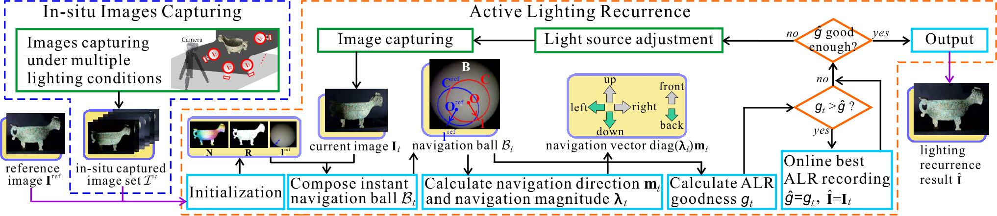
Thanks to the simplicity of ALR-apl model, it is possible to online calculate both the navigation direction and magnitude from the reference and current image, and . Fig. 2 shows the working flow of the ALR-apl approach. Specifically, to get a reliable initialization, we first roughly capture different side lighting images to form the in-situ captured image set . From and , we obtain scene normal , reflectance and reference lighting vector . Then, in each ALR-apl iteration, we compose an instant navigation ball and online calculate the navigation direction and magnitude for light source adjustment. We analyze the convergence and efficacy of this process at last.
IV-A Initialization
By parallel lighting analogy, we have
| (7) |
where is shading image that can be obtained by disambiguated intrinsic image decomposition [41], by solving . Clearly, from and , we can obtain shading images and we use them to calculate the scene normal and reference (target) lighting vector (i.e., in Eq. (5)) via a fast state-of-the-art uncalibrated photometric stereo algorithm, LDR [25]. Considering that the change occurred in scene is tiny, here we omit the influence of time interval on scene, i.e., 22 2 The simplification about scene information is only for estimating reference lighting condition , since both and are all real images captured by camera, the change can be reproduced in the currently captured images.. In practice, we only need side lighting images for initialization.
IV-B Instant navigation ball
Given and , the lighting vector corresponding to the current image can be easily obtained by solving Eq. (7) in closed-form solution. To eliminate scene dependency in ALR process, we online render both current and reference lightings, and , onto a unit sphere, rather than on the real scene normal . Specifically, let and be the reference and currently rendered images of the unit sphere, i.e., and , where is the sphere normal which is known. From the Lambertian law, we can easily obtain the following proposition about the spherical isointensity sets and , formed by rendered pixels with some particular intensity value, e.g., the median of .
Proposition 1 (SICs & shading equivalence).
With analogy parallel lighting and Lambertian law, given an arbitrary lighting vector , the spherical isointensity set always forms a circle under the view of lighting direction, which can be named as spherical isointensity circle (SIC). Iff the reference and current SICs, and coincide completely, the reference and current images, and , are the same.
Proof.
SICs: For Eq. (7), we replace by a sphere normal . For arbitrary point , we have
| (8) |
where is the included angle of and . Given two points and which satisfy and , we have
| (9) |
It means that if any two points on the rendered image have the same intensity, the normals of the two points have the same angle with . In other words, the points having identical intensity value on , i.e., the spherical isointensity set forms a circle under the view of the parallel lighting direction.
Shading equivalence: We first prove the sufficient condition. For each pixel in (and ) on (and ), we have and . Considering , so . Therefore, only if contains more than three spherical points, the linear system leads to . Furthermore, since scene normal and reflectance remain the same, the real captured images are fully determined by the lighting condition. Thus, we have . The proof of necessary condition is similar to the sufficient condition and we do not provide the details. ∎

Proposition 1 means that ALR is finished if we can make the reference and current SICs, and coincide by adjusting light source pose. As shown in Fig. 4, we dynamically compose an instant navigation ball to provide effective instant ALR navigation for adjusting light source,
| (10) |
where is the current rendered image, and are the center coordinates of and , respectively. Essentially, the navigation ball provides a visual navigation guidance in th iteration, which can be used to calculate the navigation direction and magnitude.
IV-C Online calculation of navigation direction

As shown in Fig. 4, since and encode the lighting direction of light source in the azimuthal and polar axes respectively, an analogy parallel light source pose can be expressed by vector in the spherical coordinate frame, with being the distance between the light source and the coordinate frame center. Therefore, we can effectively calculate the ALR navigation direction in radial, azimuthal and polar axes according to ,
| (11) |
where and are the areas of SICs and , respectively, denotes region area, is the sign function. In fact, the area of SIC encodes the distance information between light source and coordinate frame center. As illustrated by Fig. 4, reflects the positive () or negative () ALR directions respectively along the three axes of spherical coordinate, for the apl model.
IV-D Online calculation of navigation magnitude
With real-time calculation of current navigation direction , we can establish a manual control loop with as desired set-point (SP) and being the measured process variable (PV). For many real-world fine-grained change detection tasks, manual ALR, or ALR with hand (ALR_H), is reliable due to its great portability.
Nevertheless, as shown in Fig. 4, we can also effectively calculate the ALR navigation magnitude via bisection approaching, which together with can enable an automatic ALR process, with the help of a robotic platform (ALR_R). Specifically, given an initial , where , and indicate the initial light source adjustment magnitude in radial, azimuthal and polar axes, respectively. In th () ALR iteration, satisfies
| (12) |
where denotes the three independent spherical axes, is the speed-up rate of navigation magnitude and is empirically set as in our experiments. With Eq. (12), we can efficiently obtain the ALR navigation vector, i.e., ALR increment , which is directly applied on the robotic platform to conduct the th ALR adjustment.
IV-E The algorithm and implementation details
Algorithm 1 shows the detailed working flow of our ALR-apl approach. Specifically, in th iteration, we first compose the navigation ball according to and , then calculate the navigation direction and navigation magnitude . After that, we adjust light source pose by . This iterative adjustment process is terminated by an ALR goodness that measures the recurrence accuracy by the overlap ratio, i.e., the Intersection-over-Union (IoU) of and ,
| (13) |
where and indicate the regions inclosed by and respectively, is region area. During ALR, we record the largest and the corresponding current image by and , respectively. Once , is just the final lighting recurrence result. We set to and we use the median of reference rendered image to form and . We empirically set mm in our experiments.
IV-F Convergence analysis
Eq. (12) indeed defines a bisection approaching strategy. We can see that the light source pose adjustments in the three spherical axes are independent of one another. In th iteration, we physically adjust the light source pose by , which is calculated by Eq. (11) and Eq. (12). After multiple adjustments, the light source finally reaches the target pose, i.e., ALR is finished. See the green curve of Fig. 4 for an example of light source adjustment trajectory. Hence, the convergence of the ALR process relies on .
Lemma 1 (Convergence of ).
Using the bisection approaching strategy, i.e., Eq. (12), if bisection occurs infinite times, we have if .
Proof.
We have and we first prove the convergence of . As shown in Fig. 5(a), we assume the light source has been adjusted to along the radial-axis from initial pose , and the light source should cross the reference pose at next iteration . Note, the solid and dashed lines indicate the adjustments that have and have not yet occurred, respectively. Then, we have the conclusion that if , Fig. 5(b) (or (c)) and Fig. 5(d) (or (e)) happen alternately. Specifically, after th iteration, i.e., Fig. 5(a), then Fig. 5(b) or (c) must happen and followed by Fig. 5(d) or (e), and Fig. 5(b) or (c) happens once again after that. The alternation process lasts forever. Note, here we only consider . If , the above alternation process may not be satisfied. For Fig. 5(b) or (d), we have
| (14) |
where . Similarly, for Fig. 5(c) or (e), we have
| (15) |
where is the speed-up rate of navigation magnitude. Therefore, for th iteration (), we have
| (16) |
where and denote the occurrence times of Eq. (14) and Eq. (15), respectively. In fact, . Since is finite, when approaches infinity, and also approach infinity. Hence, we have if . The convergence proof of or is same to and we don’t provide the details here. Then, we have when . ∎
According to Lemma 1, we have . Fig. 6 demonstrates the convergence process of the navigation vector under different speed-up rate by simulation experiment. We set the target light source pose, initial light source pose and initial navigation magnitude to , and , respectively. Then we conduct ALR under different speed-up rates. From Fig. 6, we can find that, (, in Fig. 6) may effectively help the light source to quickly approach the target and accelerate the convergence compared with . Besides, Fig. 6 also verifies that ALR does not converge if . In fact, the selection of is related to many factors, e.g., scene, initial light source pose, initial navigation magnitude of ALR. Empirically, we set to in our experiments.
IV-G Invariance to and decomposition ambiguity
According to Eq. (7), the and decomposition generally subjects to an ambiguity matrix satisfying , where and are the real normal and lighting vector. Therefore, our initialization also exits an ambiguity matrix between the calculated and real lighting vectors (or scene normals), which may influence the correctness of ALR. Fortunately, we prove that if the angle difference between and is not larger than , the ambiguity matrix does not affect the effectiveness and convergence of our ALR approach.
Lemma 2.
The ambiguity matrix generated by the decomposition of Eq. (7) is a rotation matrix.
Proof.
Since is a full rank linear system, has a unique solution. Since both and are row unit vectors for any point , there is a rotation matrix satisfying , then , i.e., is a rotation matrix. ∎
Lemma 3.
The ALR navigation guidance in radial-axis is independent to .
Proof.
From Proposition 1, we know that for any point in SIC , and have the same included angle . We have
| (17) |
Let be the radius of , then the area of satisfies
| (18) |
Since , combining Eq. (17) and Eq. (18), we have . Since the intensities of all points in reference SIC and current SIC are the same, so . We can see , where denotes the operator in , i.e., and have the same magnitude relation. Besides, we know and . It means and have the same magnitude relation to ground truth and . Thus, the ambiguity matrix does not influence the ALR navigation in radial direction. ∎
Lemma 4.
Let be the axis-angle representation of . For the azimuthal and polar direction in Eq. (11), if , does not affect our ALR process. We can faithfully relocalize the light source to reference apl pose.
Proof.
The azimuthal and polar adjustments of light source on sphere only cause the change of lighting direction. Since we use the same and to calculate and , it satisfies and , where and are the real reference and current lighting vectors. From Fig. 3(d), we have
| (19) |
where denotes th iteration, rotation matrix denotes the matrix form of navigation from current lighting to the reference one, is the real light source adjustment realized by robotic platform or hand. From Eq. (19), we have . Generally, we pursue to adjust light source by , i.e., . So, . From Theorem 1 of [14], we know infinitely approaches unit matrix if , i.e., and are coincided. Since and , and are coincided too. Hence, we can say that users can always relocalize the light source to the reference pose if . ∎
The convergence condition of in Lemma 4 is equivalent to the one of lighting vector, i.e., if the angle difference between and is not larger than , does not affect the convergence of our ALR-apl. In fact, the convergence condition can be easily satisfied by current photometric stereo methods [25], which is empirically verified and discussed in detail in Sec. VI-B.
V ALR under More Realistic Lighting
In fact, ideal parallel lighting is inexistent in the real world. The commonly-used realistic light sources include near point light (NPL) source and small near surface light (sNSL) source. However, the NPL model or sNSL model usually cannot satisfy the requirement of real-time navigation response of ALR, because of the model’s sophistication. Fortunately, in this paper, we prove that using the proposed ALR-apl method can also be applied to the above two kinds of light sources.
V-A ALR under near point lighting
From Fig. 3(b), near point lighting assigns different scene points with distance-related lighting directions,
| (20) | ||||
where is the shading image, is the near point light source position, indicates the spatial coordinate of point , is the lighting power.
Proposition 2 (SICs & shading equivalence).
Under NPL model, Given an arbitrary near point light source position, the spherical isointensity set acquired from the rendered image always forms a circle, under the view that light source points to the sphere center. Iff the reference and current SICs and coincide completely, the reference and current images, and , are the same.
Proof.
SICs: We replace by a sphere normal . Let be the light source position. From Fig. 3(b), we have
| (21) |
where indicates the lighting vector and satisfies , represents the distance between and , denotes the included angle between and . Since and have the same magnitude relation, thus
| (22) |
So we have the same conclusion like Proposition 1, i.e., the spherical isointensity set forms a circle under the view that the point light source towards the sphere center.
Shading equivalence: We first prove the sufficient condition. For each pixel in (and ) on (and ), we have and . Since , . Refer to Proposition 1, and have the same magnitude relation, we have , then
| (23) | ||||
Since Eq. (23) holds for any point in and , we have , i.e., the reference and current positions of near point light source are the same, so . The proof of necessary condition is similar to the sufficient condition and we do not provide the details. ∎
Proposition 3 (ALR navigation equivalence).
The ALR approach for the apl model is also applicable to NPL model.
Proof.
As shown in Fig. 3(b), there is an approximate parallel lighting which parallels to the direction that the NPL towards sphere center. We use superscripts ‘apl’ and ‘npl’ to distinguish the two models. Given any two points and , it satisfies
| (24) | ||||
where denotes an operator in . That is, and have the same magnitude relation. Thus, combining Proposition 2, the proposed ALR-apl strategy can also be applied to near point lighting condition. ∎
V-B ALR under small near surface lighting
Refer to Fig. 3(c), a small near surface light source (sNSL) can be seen as the combination of many near point light sources. Thus, under sNSL model, we have
| (25) | ||||
where indicates the th near point light source, denotes the lighting power of all NPLs, is the number of NPLs, indicates the spatial coordinate of point . We can find that solving from Eq. (25) is a nonlinear problem which is hard to be solved. Replacing the scene normal by the sphere normal , we have
| (26) |
where indicates the lighting vector that th scene point towards th NPL, and it satisfies . As shown in Fig. 7(a), generally, the size of sNSL is much less than the distance between sNSL and the scene center. Besides, we take no account of the rotation of sNSL and keep the sNSL midperpendicular always pointing to the scene center during ALR process. Under these constraints, we can approximatively consider that each NPL in sNSL has the same distance to a certain scene point , i.e., , where is the lighting vector that sNSL center points to scene point . Then we rewrite Eq. (26) as
| (27) |
Refer to Fig. 7(b), we have
| (28) |
where , and indicates the coordinate of sNSL center. According to Eq. (28), we can get . Then we rewrite Eq. (27) as
| (29) |
We can see that is a constant and Eq. (29) has the same form with Eq. (21), so the sNPL can be seen as a NPL, and the spatial coordinate is . Similar to the propositions about NPL, we can take the conclusion that the ALR-apl method can be applied to sNSL condition directly.
VI Experimental Results

VI-A Setup
We build 13 different scenes (S1–13) for evaluating the proposed ALR method. S1–3, S11 and S13 mainly exhibit near-Lambertian surface. The other scenes involve some non-Lambertian regions, e.g., transparency (S4, S12), hard cast shadow (S5–6) and specularity (S7–10, S12). See Fig. 8, we use a small lamp bulb and a small handheld LED surface light source as the near point light (NPL) source and small near surface light source (sNSL), respectively. Besides, we employ a consumer robotic arm (uArm Swift Pro) to verify the effectiveness of the automatic ALR. All images are captured by a Canon 5D Mark III camera. Experiments are conducted in a consumer computer with i7 CPU.
VI-B Convergence and effectiveness validation
Refer to Eq. (12), we use a bisection approaching strategy to calculate the navigation vector for th iteration of ALR. To verify the convergence of navigation vector, we conduct ALR using the robotic arm for scenes S4 and S5, then we record the navigation vector of each iteration. Fig. 9 shows the relation of the navigation vector (absolute value) and the iteration number for the two scenes. We can clearly see that the navigation direction is alternately changed during ALR process, and the navigation magnitude increases in the beginning and then gradually converges to zero. See Sec. IV-F for the convergence proof of navigation vector.
We use the ALR goodness , i.e., the Intersection-over-Union (IoU) as the termination condition for ALR process. To verify the effectiveness, we conduct ALR using the robotic arm for S1 and S7, and we record the image and the corresponding for each iteration. Then we calculate the SSIM and MS-SSIM [42] scores for each image. Fig. 10(a)–(b) show the relation of ALR goodness and the (MS-)SSIM score. Besides, the 10-times magnified absolute differences between the reference image and some captured images during ALR are also shown. Since the slight change of lighting condition may cause large difference of image appearance, it is reasonable that the (MS-)SSIM decreases slightly sometimes (see the variation tendency of (MS-)SSIM in Fig. 10(b)). Nevertheless, the (MS-)SSIM increases with the increase of on the whole.

Refer to Sec. IV-G, we prove that if the angle difference between and is not larger than , the ambiguity matrix does not affect the convergence of our ALR approach. In fact, the condition is easy to be met. To verify this, we introduce the dataset [43] which includes 7 statue scenes (e.g., Cat, Frog, Hippo) and corresponding ground truth normals. Each scene has 20 multi-illumination images. We calculate the scene normal by LDR [25] and calculate the mean angle error (MAE) for each scene. The MAE scores are shown in Table I. We find that these MAEs are much less than . Therefore, according to Lemma 4, we can confidently say that the ambiguity matrix does not influence our ALR method.
| Scene | Cat | Frog | Hippo | Lizard | Pig | Scholar | Turtle |
|---|---|---|---|---|---|---|---|
| MAE |
The proposed ALR method only need a small amount of in-situ captured images for initialization. To verify this, we conduct ALR using robotic arm for S1–5 with different numbers of in-situ images. The 2nd to 5th rows of Table II show the averages of 4 commonly-used image similarity criteria, i.e., MSE, PSNR, SSIM and MS-SSIM [42] under different image numbers. The 6th row of Table II shows the mean angle error (MAE) between the calculated scene normal and the one using 100 images. We can see the MAE reduces with the increase of image number, and the recurrence accuracy of ALR is stable and always well. In fact, our ALR method is effective as long as the calculated scene normal satisfies Lemma 4, and more images cannot help to improve the recurrence accuracy. Empirically, we use 13 multi-illumination images for calculating scene normal and reflectance.
| # Imgs | 5 | 10 | 20 | 40 | 60 | 80 | 100 |
|---|---|---|---|---|---|---|---|
| MSE | 3.4289 | 3.2433 | 2.5803 | 2.8792 | 2.6086 | 2.7137 | 2.8708 |
| PSNR | 42.7792 | 43.0208 | 44.0140 | 43.5379 | 43.9665 | 43.7950 | 43.5506 |
| MSSSIM | 0.9953 | 0.9953 | 0.9961 | 0.9957 | 0.9961 | 0.9960 | 0.9957 |
| MS_MSSIM | 0.9964 | 0.9964 | 0.9967 | 0.9965 | 0.9967 | 0.9966 | 0.9966 |
| MAE | 0 |
VI-C Quantitative comparison
To compare with our ALR method, we use the small lamp bulb (NPL) and the small handheld LED surface light source (sNSL) to collect 13 multi-illumination images as the reference images for scenes S1–10 and scenes S11–13, respectively. We recur all the 13 side lightings using our ALR method for all scenes by hand (ALR_H). Considering the robotic arm only has 3 degrees of freedom and it cannot keep the sNSL always towards the scene center, so we only conduct ALR with robotic arm (ALR_R) for S11–13. We use PTM [4], HSH [5], LDR [25] as the baselines. PTM [4] and HSH [5] are two image-based relighting methods. For PTM and HSH, we use a light probe to calibrate the lighting direction for each captured image. LDR [25] is a state-of-the-art uncalibrated photometric stereo method based on parallel lighting model. We carry out the 3 methods using the captured 13 images and generate 13 lighting recurrence images. We use MSE, PSNR, SSIM, MS-SSIM [42] as accuracy metrics.
Fig. 11 and Fig. 12 show the quantitative comparisons of our ALR method and 3 baselines for scenes S1–10 and S11–13, respectively. Each node indicates the average evaluation of 13 lighting recurrence results and the up and down bar of each node denotes the variance. The average of each method for all scenes are also shown in Fig. 11 and Fig. 12. Besides, all the scores of the 4 criteria for each scene can be approached in Tables III–VI. We can see that our method ALR_R or ALR_H can achieve the best recurrence accuracy than baselines. Besides, from Tables III–VI, we can find the evaluation scores of ALR_R are slightly better than ALR_H except for S8. This is because the light source adjustment by robotic arm is more stable than hand and it is more easy to get more accuracy recurrence results for robotic arm.
| Method | S1 | S2 | S3 | S4 | S5 | S6 | S7 | S8 | S9 | S10 | S11 | S12 | S13 |
|---|---|---|---|---|---|---|---|---|---|---|---|---|---|
| PTM | 3.89 | 7.83 | 12.49 | 11.39 | 19.33 | 8.39 | 10.32 | 6.41 | 14.60 | 19.28 | 25.16 | 28.82 | 27.36 |
| HSH | 118.16 | 72.12 | 70.67 | 244.34 | 92.67 | 154.44 | 105.54 | 68.31 | 239.28 | 102.20 | 56.88 | 54.700 | 32.31 |
| LDR | 3.27 | 16.10 | 35.41 | 21.57 | 49.18 | 19.31 | 26.77 | 22.61 | 29.86 | 61.27 | 82.50 | 58.79 | 32.02 |
| ALR_H | 1.75 | 4.57 | 9.16 | 4.39 | 6.72 | 2.36 | 7.72 | 5.21 | 8.81 | 6.59 | 10.10 | 2.70 | 1.44 |
| ALR_R | 1.19 | 4.07 | 8.08 | 2.66 | 3.48 | 2.14 | 6.04 | 5.64 | 4.48 | 6.13 | NA | NA | NA |
| Method | S1 | S2 | S3 | S4 | S5 | S6 | S7 | S8 | S9 | S10 | S11 | S12 | S13 |
|---|---|---|---|---|---|---|---|---|---|---|---|---|---|
| PTM | 42.45 | 39.34 | 37.30 | 38.46 | 35.75 | 39.36 | 38.11 | 40.26 | 36.68 | 35.59 | 34.29 | 34.11 | 34.34 |
| HSH | 27.58 | 29.96 | 30.00 | 24.35 | 28.89 | 26.37 | 28.02 | 30.02 | 24.50 | 28.30 | 30.67 | 31.25 | 33.90 |
| LDR | 43.10 | 36.29 | 32.72 | 35.76 | 31.54 | 35.66 | 34.00 | 34.82 | 33.58 | 30.53 | 29.19 | 31.11 | 33.61 |
| ALR_H | 45.71 | 41.56 | 38.53 | 41.97 | 39.89 | 44.44 | 39.26 | 41.07 | 38.77 | 39.98 | 38.12 | 44.03 | 46.64 |
| ALR_R | 47.39 | 42.04 | 39.07 | 44.08 | 42.76 | 44.91 | 40.34 | 40.70 | 41.69 | 40.29 | NA | NA | NA |
| Method | S1 | S2 | S3 | S4 | S5 | S6 | S7 | S8 | S9 | S10 | S11 | S12 | S13 |
|---|---|---|---|---|---|---|---|---|---|---|---|---|---|
| PTM | 0.9841 | 0.9788 | 0.9803 | 0.9745 | 0.9738 | 0.9710 | 0.9819 | 0.9793 | 0.9787 | 0.9756 | 0.9585 | 0.9618 | 0.9572 |
| HSH | 0.7469 | 0.7467 | 0.7758 | 0.4727 | 0.7212 | 0.3762 | 0.6407 | 0.6982 | 0.6735 | 0.8020 | 0.9215 | 0.9044 | 0.9337 |
| LDR | 0.9800 | 0.9601 | 0.9606 | 0.9649 | 0.9560 | 0.9473 | 0.9704 | 0.9561 | 0.9610 | 0.9546 | 0.9219 | 0.9294 | 0.9386 |
| ALR_H | 0.9914 | 0.9913 | 0.9939 | 0.9885 | 0.9924 | 0.9905 | 0.9913 | 0.9916 | 0.9879 | 0.9922 | 0.9924 | 0.9930 | 0.9936 |
| ALR_R | 0.9918 | 0.9918 | 0.9945 | 0.9903 | 0.9940 | 0.9906 | 0.9918 | 0.9915 | 0.9916 | 0.9925 | NA | NA | NA |
| Method | S1 | S2 | S3 | S4 | S5 | S6 | S7 | S8 | S9 | S10 | S11 | S12 | S13 |
|---|---|---|---|---|---|---|---|---|---|---|---|---|---|
| PTM | 0.9955 | 0.9942 | 0.9954 | 0.9908 | 0.9915 | 0.9918 | 0.9954 | 0.9946 | 0.9900 | 0.9893 | 0.9891 | 0.9821 | 0.9859 |
| HSH | 0.9718 | 0.9818 | 0.9799 | 0.9152 | 0.9781 | 0.9266 | 0.9737 | 0.9661 | 0.9608 | 0.9765 | 0.9765 | 0.9682 | 0.9836 |
| LDR | 0.9942 | 0.9878 | 0.9875 | 0.9856 | 0.9820 | 0.9846 | 0.9907 | 0.9872 | 0.9793 | 0.9754 | 0.9680 | 0.9646 | 0.9796 |
| ALR_H | 0.9958 | 0.9959 | 0.9970 | 0.9946 | 0.9965 | 0.9954 | 0.9957 | 0.9958 | 0.9939 | 0.9962 | 0.9962 | 0.9965 | 0.9968 |
| ALR_R | 0.9961 | 0.9961 | 0.9972 | 0.9953 | 0.9973 | 0.9955 | 0.9959 | 0.9957 | 0.9959 | 0.9963 | NA | NA | NA |
Fig. 13 shows the recurrence results using NPL for several typical scenes S2 (near-Lambertian), S4 (transparent), S6 (cast shadow) and S9 (specular), including the zoom-in regions and corresponding 10-times magnified absolution difference images. Similarity, Fig. 14 shows the recurrence results for S11 (near-Lambertian) and S12 (transparent & specular) using sNSL. We can see that our method ALR_H or ALR_R can generate more accurate lighting recurrence results than baselines for both quantitative comparison and visual perception. Furthermore, see Fig. 13 and Fig. 14, although PTM and LDR can also achieve not bad recurrence results for the near-Lambertian scenes, they cannot do well for the non-Lambertian scenes. This is because the non-Lambertian regions are usually more hard to reproduce than near-Lambertian regions for these SLR methods. Thanks to the physical lighting recurrence, although our ALR method is based on Lambertian assumption, it can still achieve excellent lighting recurrence accuracy for non-Lambertian scenes.


VI-D Speed comparison
The proposed ALR method can generate real-time navigation feedback for adjusting light source. Table VII shows the FPSs of our ALR method under different image sizes. Since the cannon 5D Mark III camera we used cannot acquire the real-time original image (57603840), we just use the live view image (960640) and perform downsampling by 2 (480320) to support light source navigation in our experiments. After ALR, we capture the 57603840 image as the finial lighting recurrence image. Besides, We record the average time of ALR with hand (ALR_H) and robotic arm (ALR_R). It takes about s for ALR_H and s for ALR_R in our experiments (exclude the time of image capturing and initialization). For ALR_H, we can quickly adjust the light source to a local range of the target but it is not easy to achieve a better recurrence accuracy because of the instability of manual adjustment. In contrary, since the robotic arm cannot percept the scene, ALR can only rely on the bisection adjustment strategy to adjust light source, so the light source cannot be rapidly adjusted to approach the target in the beginning. But as the light source approaches the target, the advantage of movement stability of robotic arm can help it to achieve higher accuracy.
| Size (pixel) | 9664 | 192128 | 288192 | 384256 | 480320 |
|---|---|---|---|---|---|
| FPS | 33.0961 | 27.2844 | 18.2382 | 13.7874 | 9.7125 |
| Size (pixel) | 576384 | 672448 | 768512 | 864576 | 960640 |
| FPS | 7.5620 | 5.8763 | 4.6747 | 3.7234 | 3.0444 |
VI-E ALR under multiple light sources
Up to now, what we have discussed is the ALR under single light source. In fact, using multiple light sources can effectively achieve higher imaging quality and capture more rich scene microstructures than single light source. Except for fine-grained change monitoring and measurement, ALR under multiple light sources is also useful in many other fields, e.g., lighting re-setup for photography, which usually needs to reproduce a specific light source combination to express some character emotion or photography style [44]. Fortunately, without any auxiliary, our ALR method can be directly applied to multiple light sources condition. Specifically, in the reference observation, we successively lighten each light source and capture the corresponding image. Then, during current observation, we also successively conduct ALR for each light source, using the corresponding image as the reference. Note, for each ALR, the light sources which have been relocated are regarded as the environment lighting. To verify the effectiveness, we conduct ALR under two near point light sources by two robotic arms for scene S3–5. The results are shown in Fig. 15. For each case, the first row indicates the two reference images, the second row denotes the ALR results. The recurred image and the 10-times magnified absolute differences are also shown in Fig. 15. We can find the ALR results faithfully reproduce the scene surface details of the reference one.

VII Real-World Applications

One promising application of the proposed ALR method is accurately capturing fine-grained change of high-value objects. For instance, in cultural heritage conservation, an essential problem is to detect and measure the minute changes of cultural relics from two sets of observations within long time intervals. This is an open real-world problem since cultural relics (e.g., Dunhuang Mogao murals) suffer from various of deteriorations even though they have been seriously protected. However, this is a quite tough problem, and challenges particular from misaligned image position as well as misaligned lighting condition. In addition, some changes can only be clearly observed in specific lighting condition so that ALR is of great importance in fine-grained change detection problem.
To address this problem, we combine our ALR method with the high-accurate actively camera relocalization method (ACR) [14] and a state-of-the-art fine-grained change detection method (FGCD) [6]. We apply our ALR to actively capture and measure the fine-grained changes of ancient murals in two World Cultural Heritage Sites, Dunhuang Mogao Grottoes (Case 1–5) and Weijin Graves (Case 6–9) in Fig. 16. Specifically, given the reference image, we first relocalize current camera pose via ACR, then we do ALR to physically reproduce the lighting condition of reference image and take current images for evaluation. The time interval between twice observations is one year for Case 1–2 and Case 6–9, and 12 days for Case 3–5. Besides, we also capture 20 images under different lighting conditions in current observation and carry on PTM [4] to generate relighting images for comparison. Fine-grained changes are detected by FGCD algorithm for both ALR and PTM results.
All the results are shown in Fig. 16. Refer to the zoom-in regions and corresponding FGCD results, we can clearly see that our ALR can generate much higher F1-Measure and lower FPR errors. This is because that some surface details cannot be faithfully reproduced by PTM, e.g., the cast shadow region of Case 2 in Fig. 16. Note, for some scenes, e.g., Case 1, there is no change between twice observations, so we show the FPR value instead of F1-Measure. In a word, our ALR supports much more accurate fine-grained change detection.
VIII Conclusion
In this paper, we have studied a new problem, active lighting recurrence (ALR), that aims to actively reproduce the lighting condition of a single reference image. To achieve instant and accurate ALR guidance, we propose a simple yet effective analogy parallel lighting (apl) based ALR approach. We show that the proposed approach works well for the commonly-used realistic near point light source and small near surface light source, with strict theoretical equivalence and convergence guarantees. Besides, we also prove the invariance of our approach to the ambiguity of normal and lighting decomposition. To the best of our knowledge, this is the first solid ALR study in computer vision and robotics.
ALR plays a crucial role in real-world fine-grained change detection (FGCD) tasks of cultural heritages. Different with existing synthetic lighting recurrence (SLR), our ALR guarantees the physical correctness of the recurrence image and can be conducted in real-time. Besides, our method supports both manual operation and robotic platform, i.e., has strong environmental adaptability. So far, our approach has been successfully applied to a number of real-world FGCD tasks, e.g., for the first time, we discover the minute change in less than 2 weeks time interval in Dunhuang Mogao Grottoes.
In this work, we propose the new ALR problem and achieve an effective ALR method. Our work provides a useful and novel research topic in active robotic vision, which is the significance of this paper. In fact, our work is just a beginning of ALR problem. In the future, we plan to further study ALR with different light source types and under varied environment lightings during twice observations.
References
- [1] P. Debevec, T. Hawkins, C. Tchou, H. Duiker, W. Sarokin, and M. Sagar, “Acquiring the reflectance field of a human face,” in ACM SIGGRAPH, 2000.
- [2] Y. Chuang, D. Zongker, J. Hindorff, B. Curless, D. Salesin, and R. Szeliski, “Environment matting extensions: Towards higher accuracy and real-time capture,” in ACM SIGGRAPH, 2000.
- [3] J. Ou and F. Pellacini, “LightSlice: Matrix slice sampling for the many-lights problem,” ACM TOG, vol. 30, no. 6, pp. 179:1–179:8, 2011.
- [4] M. Tom, G. Dan, and W. Hans, “Polynomial texture maps,” in ICME, 2001.
- [5] S. Elhabian, R. Ham, and A. Farag, “Towards accurate and efficient representation of image irradiance of convex-lambertian objects under unknown near lighting,” in ICCV, 2011.
- [6] W. Feng, F. Tian, Q. Zhang, N. Zhang, L. Wan, and J. Sun, “Fine-grained change detection of misaligned scenes with varied illuminations,” in ICCV, 2015.
- [7] R. Huang, W. Feng, Z. Wang, M. Fan, L. Wan, and J. Sun, “Learning to detect fine-grained change under variant imaging conditions,” in ICCVW, 2017.
- [8] P. Ren, Y. Dong, S. Lin, X. Tong, and B. Guo, “Image based relighting using neural networks,” in ACM SIGGRAPH, 2015.
- [9] S. Liu and M. Do, “Inverse rendering and relighting from multiple color plus depth images,” IEEE TIP, vol. 26, no. 10, pp. 4951–4961, 2017.
- [10] X. Huang, M. Walton, G. Bearman, and O. Cossairt, “Near light correction for image relighting and 3d shape recovery,” in Digital Heritage, 2015.
- [11] B. Shi, Z. Wu, Z. Mo, D. Duan, S.-K. Yeung, and P. Tan, “A benchmark dataset and evaluation for non-Lambertian and uncalibrated photometric stereo,” in CVPR, 2016.
- [12] K. Midorikawa, T. Yamasaki, and K. Aizawa, “Uncalibrated photometric stereo by stepwise optimization using principal components of isotropic brdfs,” in CVPR, 2016.
- [13] S. Staniforth, Ed., Historical Perspectives on Preventive Conservation. Getty Conservation Institute, 2013.
- [14] F.-P. Tian, W. Feng, Q. Zhang, X. Wang, J. Sun, V. Loia, and Z.-Q. Liu, “Active camera relocalization from a single reference image without hand-eye calibration,” IEEE TPAMI, 2018.
- [15] Q. Zhang, W. Feng, L. Wan, F.-P. Tian, and P. Tan, “Active recurrence of lighting condition for fine-grained change detection,” in IJCAI, 2018.
- [16] W. Feng, F. Tian, Q. Zhang, and J. Sun, “6D dynamic camera relocalization from single reference image,” in CVPR, 2016.
- [17] Y. Shi, F. Tian, D. Miao, and W. Feng, “Fast and reliable computational rephotography on mobile device,” in ICME, 2018.
- [18] D. Miao, F. Tian, and W. Feng, “Active camera relocalization with RGBD camera from a single 2D image,” in ICASSP, 2018.
- [19] F. Lu, I. Sato, and Y. Sato, “Uncalibrated photometric stereo based on elevation angle recovery from BRDF symmetry of isotropic materials,” in CVPR, 2015.
- [20] X. Huang, E. Uffelman, O. Cossairt, M. Walton, and A. Katsaggelos, “Computational imaging for cultural heritage: Recent developments in spectral imaging, 3-d surface measurement, image relighting, and x-ray mapping,” IEEE Signal Processing Magazine, vol. 35, no. 5, pp. 130–138, 2016.
- [21] R. Woodham, “Photometric method for determining surface orientation from multiple images,” Optical engineering, vol. 19, no. 1, 1980.
- [22] W. Silver, “Determining shape and reflectance using multiple images,” in MIT, 1980.
- [23] B. Shi, P. Tan, Y. Matsushita, and K. Ikeuchi, “A biquadratic reflectance model for radiometric image analysis,” in CVPR, 2012.
- [24] S. Ikehata and K. Aizawa, “Photometric stereo using constrained bivariate regression for general isotropic surfaces,” in CVPR, 2014.
- [25] P. Favaro and T. Papadhimitri, “A closed-form solution to uncalibrated photometric stereo via diffuse maxima,” in CVPR, 2012.
- [26] R. Basri, D. Jacobs, and I. Kemelmacher, “Photometric stereo with general, unknown lighting,” IJCV, vol. 72, no. 3, 2007.
- [27] F. Sakaue and J. Sato, “A new approach of photometric stereo from linear image representation under close lighting,” in ICCV, 2011.
- [28] W. Xie, C. Dai, and C. Wang, “Photometric stereo with near point lighting: A solution by mesh deformation,” in CVPR, 2015.
- [29] H. Nguyen and M. Do, “Inverse rendering of lambertian surfaces using subspace methods,” TIP, vol. 23, no. 12, 2014.
- [30] T. Hawkins, P. Einarsson, and P. Debevec, “A dual light stage,” in Rendering Techniques, 2005.
- [31] B. Choudhury and S. Chandran, “A survey of image-based relighting techniques,” Journal of Virtual Reality and Broadcasting, vol. 4, no. 7, 2007.
- [32] P. Peers, D. Mahajan, B. Lamond, A. Ghosh, W. Matusik, R. Ramamoorthi, and P. Debevec, “Compressive light transport sensing,” ACM TOG, vol. 28, no. 1, p. 3, 2009.
- [33] P. Sen and S. Darabi, “Compressive dual photography,” Computer Graphics Forum, vol. 28, no. 2, pp. 609–618, 2009.
- [34] D. Reddy, R. Ramamoorthi, and B. Curless, “Frequency-space decomposition and acquisition of light transport under spatially varying illumination,” in ECCV, 2012.
- [35] M. Fuchs, V. Blanz, and H. Seidel, “Bayesian relighting,” in EGSR, 2005.
- [36] M. O’Toole and K. Kutulakos, “Optical computing for fast light transport analysis,” ACM TOG, vol. 29, no. 6, p. 164, 2010.
- [37] M. Fuchs, V. Blanz, H. Lensch, and H. Seidel, “Adaptive sampling of reflectance fields,” ACM TOG, vol. 26, no. 2, p. 10, 2007.
- [38] D. Nowrouzezahrai and J. Snyder, “Fast global illumination on dynamic height fields,” Computer Graphics Forum, vol. 28, no. 4, pp. 1131–1139, 2009.
- [39] P. Ren, J. Wang, M. Gong, S. Lin, X. Tong, and B. Guo, “Global illumination with radiance regression functions,” ACM TOG, vol. 32, no. 4, p. 130, 2013.
- [40] W. Ye, X. Li, Y. Dong, P. Peers, and X. Tong, “Single image surface appearance modeling with self-augmented cnns and inexact supervision,” in Computer Graphics Forum, vol. 37, no. 7. Wiley Online Library, 2018, pp. 201–211.
- [41] Q. Zhao, P. Tan, Q. Dai, L. Shen, E. Wu, and S. Lin, “A closed-form solution to retinex with non-local texture constraints,” IEEE TPAMI, vol. 34, no. 7, pp. 1437–1444, 2012.
- [42] Z. Wang, E. Simoncelli, and A. Bovik, “Multiscale structural similarity for image quality assessment,” in IEEE Asilomar Conference on Signals, Systems and Computers, 2003.
- [43] Y. Xiong, A. Chakrabarti, R. Basri, S. Gortler, D. Jacobs, and T. Zickler, “From shading to local shape,” IEEE TPAMI, vol. 1, no. 1, p. 1, 2015.
- [44] S. Begleiter, 50 Lighting Setups for Portrait Photographers: Easy-To-Follow Lighting Designs and Diagrams, Vol. 2. Amherst Media, 2014, vol. 2.