Power-Constrained Trajectory Optimization for Wireless UAV Relays with Random Requests

Much recent research has gone into studying UAVs operating in wireless networks [1, 2, 3, 4]. The primary motivation for this interest is due to the unique benefits that UAVs acting as flying base stations, mobile relays, etc., provide in improving the overall network performance over terrestrial infrastructure in terms of mobility, maneuverability, and enhanced line-of-sight (LoS) link probability [1, 2, 3, 4, 5].

Already, the literature has shown that consideration of UAV deployment strategies, in terms of optimal positioning or trajectory design, can go a long way to increase network performance of many of the useful metrics. In [6], dynamic repositioning led to increase in spectral efficiency over heuristics under both FDMA and TDMA schemes. The works of [7, 8] utilized UAVs in communication and maximized the total service time, with [7] outperforming static and random deployment methods, and [8] meeting BER requirements.

Although showing potential to improve these performance metrics, the design of UAV deployment strategies is not without challenges [1, 2, 3]. Optimal trajectory design must be formulated appropriately to incorporate realistic constraints imposed on the UAVs. Already, works such as [8, 9, 10] have gone at length to incorporate constraints on the limited onboard energy and mission times inherent to low-altitude platforms (LAPs) [1].

Despite the enormous interest in the design of UAV-assisted wireless communication networks, most of the prior work focuses on deterministic models, in which the data traffic generated by ground nodes (GNs) is known beforehand, and there are no uncertainties in the network dynamics. However, this is impractical in realistic systems, where uncertainty dominates, and random request arrivals must be accounted for. Therefore, the design of UAV-assisted communication networks with random data traffic is still an open problem.

To address this problem, our previous paper [5] considered the optimization of the UAV trajectory and communication strategy under random traffic generated by two GNs. However, that model was limited to two GNs, neglected the power consumption of the UAV, and assumed that the UAV is the destination of the data traffic. In this paper, we extend the model to densely deployed GNs that need to transmit data payloads to a backbone-connected base station; we investigate the optimal trajectory and communication strategy of the UAV, under an average power constraint on the UAV mobility.

To investigate this added complexity, we consider a scenario in which an UAV acts as a relay between multiple GNs dispersed uniformly in a circular cell and a central base station (BS), receiving transmission requests from the GNs according to a Poisson process. We formulate the problem as that of designing an adaptive trajectory, with the goal to minimize the average long-term communication delay incurred to serve the requests of the GNs, subject to a constraint on the long-term average UAV power consumption to support its mobility.

We show that the optimal trajectory in the communication phase operates according to a two-scale decision-making process, which can be efficiently optimized: in the outer decision, the UAV, given its current radius, selects a target end radius position, which balances optimally the trade-off between average long-term communication delay and power; in the inner decision, given its current radius and the selected end radius, the UAV greedily minimizes the delay and energy trade-off to serve the current request. Our numerical results reveal that during waiting phases, the UAV tends to circle at some optimal radius at an energy-efficient speed determined by the outer decision process, until receiving a new uplink transmission request. Additionally, we show that the optimal trajectory design vastly outperforms sensible heuristics in terms of delay minimization: it outperforms a static hovering scheme by roughly 50% and a mobile heuristic scheme by up to 20%, while maintaining the same average power consumption on the UAV.

The rest of the paper is organized as follows. In Sec. II, we introduce the system model, state the optimization problem, and cast it as a semi-Markov decision process; in Sec. III, we present the two-scale optimization approach; in Sec. IV, we provide numerical results; lastly, in Sec. V, we conclude the paper with some final remarks.

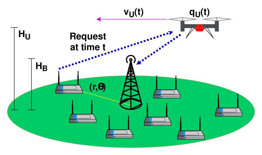
Consider the scenario depicted in Fig. 1, where multiple ground nodes (GNs) distributed uniformly over a circular cell of radius $a$ randomly generate data packets of $L$ bits, that need to be transmitted to a backbone-connected base station (BS), located in the center of the cell in position $\mathbf{q}_{B}=(0,0)$.¹¹ 1 Unless otherwise stated, we use polar coordinates to express positions, so that $\mathbf{q}=(r,\theta)$ denotes the position at distance $r$ from the center, with angle $\theta$ with respect to the $x$-axis, as shown in Fig. 1. The density of GNs within the circular radius is denoted as $\lambda_{G}$ [GNs/m²]. Each GN generates uplink transmission requests according to a Poisson process with rate $\lambda_{P}$ [requests/GN/sec]. Overall, uplink transmission requests of $L$ bits arrive in time according to a Poisson process with rate $\lambda=\lambda_{G}{\cdot}\lambda_{P}$ [requests/sec/m²]. Requests are received uniformly within the circular cell, so that the probability density function (pdf) of a request received in position $(r,\psi)$ is expressed as

Direct communication between the GNs and the BS might not be possible due to severe pathloss. An UAV is thus deployed, flying at a fixed height $H_{U}$, to relay the traffic between the GNs and the BS. Let $\mathbf{q}_{U}(t)=(r_{U}(t),\psi_{U}(t))\in\mathbb{R}_{+}\times[0,2\pi)$ be the projection of its position on the ground surface at time $t$. Due to constraints on UAV mobility, its speed is subject to a maximum constraint, expressed in polar coordinates as

where $f^{\prime}$ denotes the derivative of $f$ with respect to time.

We model the instantaneous UAV power consumption as

where $P_{\mathrm{c}}(t)$ is the total power used onboard for communication processes and $P_{\mathrm{mob}}\big(v_{U}(t)\big)$ is the forward flight mobility power, a non-convex function of the UAV speed $v_{U}(t)$ [10, 11]. We use the model in [10, 11], wherein

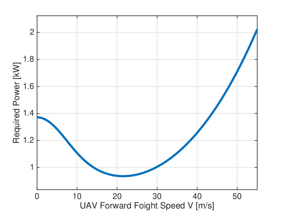
where $P_{0}$ and $P_{i}$ are scaling constants, $U_{\mathrm{tip}}$ is the rotor blade tip speed, $v_{0}$ is the mean rotor induced velocity while hovering, $\beta\triangleq d_{0}\rho sA/2$, $d_{0}$ is the fuselage drag ratio, $s$ is the rotor solidity, $\rho$ is the air density and $A$ is the rotor disc area (see [10]). An example using the physical parameters in [10] is shown in Fig. 2. Interestingly, the most power efficient operation is not achieved while hovering, but while flying at a fixed speed $V_{\min}{\simeq}20$[m/s]; in addition, it is noted that the communication power $P_{c}(t)$ (order of 1W, as in [10]) is dwarfed by the amount of power used for UAV flight, $P_{\mathrm{mob}}(V)$ (order of x$100$W). Thus in this paper we will neglect $P_{\mathrm{c}}(t)$, and approximate $P_{U}(t)\approx P_{\mathrm{mob}}\big(v_{U}(t)\big)$.

We assume that communication intervals experience line of sight (LoS) links, and that the channel faces no probabilistic elements. In fact, UAVs in LAPs generally tend to have a highly likely occurrence of LoS links [12]. When an uplink transmission request is received at time $t$ from a GN in position $(r_{G},\psi_{G})$, the communication phase begins, in which the UAV first receives the data payload from the GN, and then forwards it to the BS using a decode-and-forward, fly-hover-communicate strategy [10]. Any additional requests received during this communication phase are dropped.²² 2 Alternatively, they might be served directly from the BS. This possibility will be investigated in our future work. This phase is constituted of four distinct operations:

1. 1.

   The UAV flies from its current position $\mathbf{q}_{U}(t)=(r_{U},\psi_{U})$ to a new position $\mathbf{q}_{GU}=(r_{GU},\psi_{GU})$, at constant speed $v_{1}$; the duration of this operation is

   $$\Delta_{1}=v_{1}^{-1}\sqrt{r_{GU}^{2}{+}r_{U}^{2}{-}2r_{GU}\cdot r_{U}\cos{(\psi_{GU}{-}\psi_{U})}},$$

   (5)

   and its energy cost is $E_{1}=\Delta_{1}P_{\mathrm{mob}}\big(v_{1}\big);$

2. 2.

   The UAV hovers in position $\mathbf{q}_{GU}$ while the GN transmits its data payload of $L$ bits to the UAV; assuming a fixed transmission power $P_{\mathrm{GN}}$, the transmission rate is

   $$R_{GU}(d_{GU})\triangleq B\log_{2}\Big(1+\frac{\gamma_{GU}}{d_{GU}^{2}}\Big),$$

   (6)

   where $B$ is the channel bandwidth, $\gamma_{GU}$ is the SNR of the GN$\to$UAV link referenced at $1$-meter, and

   $$d_{GU}{=}\sqrt{H_{U}^{2}{+}r_{GU}^{2}{+}r_{G}^{2}{-}2r_{GU}\cdot r_{G}\cos{(\psi_{GU}{-}\psi_{G})}}$$

   (7)

   is the UAV-GN distance; the associated duration and energy cost are

   $$\Delta_{2}=\frac{L}{R_{GU}(d_{GU})},\ \ \ E_{2}=\Delta_{2}P_{\mathrm{mob}}\big(0\big);$$

   (8)

3. 3.

   The UAV flies from its current position $\mathbf{q}_{GU}$ to a new position $\mathbf{q}_{UB}=(r_{UB},\psi_{UB})$, at constant speed $v_{3}$; the duration of this operation is

   $$\Delta_{3}=v_{3}^{-1}\sqrt{r_{GU}^{2}{+}r_{UB}^{2}{-}2r_{GU}\cdot r_{UB}\cos{(\psi_{GU}{-}\psi_{UB})}},$$

   and its energy cost is $E_{3}=\Delta_{3}P_{\mathrm{mob}}\big(v_{3}\big);$

4. 4.

   The UAV hovers in position $\mathbf{q}_{UB}$ while it relays the data payload to the BS; assuming a fixed transmission power $P_{\mathrm{UAV}}$ and reuse of the same frequency band, the transmission rate is given by

   $$R_{UB}(d_{UB})\triangleq B\log_{2}\Big(1+\frac{\gamma_{UB}}{d_{UB}^{2}}\Big),$$

   (9)

   where $\gamma_{UB}$ is the SNR of the UAV$\to$BS link referenced at $1$-meter, $d_{UB}$ is the UAV-BS distance,

   $$d_{UB}=\sqrt{(H_{U}-H_{B})^{2}{+}r_{UB}^{2}},$$

   (10)

   and $H_{B}$ is the height of the BS antenna; the duration and energy cost of this operation are

   $$\Delta_{4}=\frac{L}{R_{UB}(d_{UB})},\ \ \ E_{4}=\Delta_{4}P_{\mathrm{mob}}\big(0\big).$$

The positions $\mathbf{q}_{GU},\mathbf{q}_{UB}$ and speeds $v_{1},v_{3}$ are part of the design. Overall, the delay and energy cost of the communication phase to serve a GN in position $(r_{G},\psi_{G})$ is given by

Once the communication phase is completed at time $t+\Delta^{(c)}$, the UAV, now in position $\mathbf{q}_{U}(t+\Delta^{(c)}){=}\mathbf{q}_{UB}$, enters the waiting phase, where it awaits for new requests, and the process is repeated indefinitely. During this process of communication and waiting for new requests, the UAV follows a trajectory, part of our design, with the goal to minimize the average communication delay, subject to an average UAV power constraint (which, given an onboard battery capacity, translates into an endurance constraint), as formulated next.

To reduce the complexity of the problem, we exploit a decomposition of the policy $\mu$, such that the total optimization problem of (26) and its dual maximization consist of solving simpler, inner and outer optimization problems separately in a two-scale decision-making approach.

Note that the steady-state pdf $\Pi_{\mu}(s)$ depends on the policy $\mu$ only through $v_{r}$ for waiting state actions $(v_{r},\theta_{c})$ and through the radius $r_{UB}$ of $\mathbf{q}_{UB}=(r_{UB},\theta_{UB})$ for communication state actions $(\mathbf{q}_{GU},v_{1},\mathbf{q}_{UB},v_{3})$. By separating $v_{r}$ from $\theta_{c}$ in the waiting states and $r_{UB}$ from the other action elements in the communication states, we have created a decomposition which allows parts of the optimal cost of a state-action pair, $\ell_{\nu}^{*}(s,\mu(s))$, to be solved separately from the steady-state probabilities $\Pi_{\mu}(s)$. Next, we formalize this decomposition.

Let $W(s)\triangleq v_{r}\in[-V_{\mathrm{max}},V_{\mathrm{max}}]$ define the radial velocity policy of the waiting states that specifies the radial velocity component of a waiting action $\mathbf{a}{=}(v_{r},\theta_{c}){\in}\mathcal{A}_{\mathrm{wait}}(r_{U})$. Additionally, let $U(s){\triangleq}r_{UB}{\in}\mathcal{R}_{\mathrm{UAV}}$ define the next radius position policy of the communication states that specifies the end radius position of the communication action. Under this decomposition, we can express the pdf $\Pi_{\mu}$ solely as a function of the policies $W,U$, i.e. $\Pi_{W,U}$, so that we have that

where $Z(s)=W(s)$ for $s\in\mathcal{S}_{\mathrm{wait}}$, $Z(s)=U(s)$ for $s\in\mathcal{S}_{\mathrm{comm}}$, and $\ell_{\nu}^{*}(s,Z(s))$ is obtained by greedily minimizing $\ell_{\nu}^{*}(s,\mathbf{a})$ with respect to the components of the actions not specified by $W,U$ (hence not affecting $\Pi_{W,U}$). Namely, for waiting states $s=(r_{U},-1,-1)$ and $W(s)=v_{r}$,

Note that the minimizer $\theta_{c}^{*}$ of (III) is the angular velocity that minimizes the UAV power consumption for some given radial velocity $v_{r}$ and UAV radius $r_{U}$, solvable offline through exhaustive search (for the case in which the power curve follows the unimodal function given in Fig. 2, it can be determined in closed form as $\theta_{c}=0$ if $v_{r}\geq v_{\min}\triangleq\arg\min_{V>0}P_{\mathrm{mob}}(V)$ and $\theta_{c}=\sqrt{v_{\min}^{2}-v_{r}^{2}}/r_{U}$ if $v_{r}<v_{\min}$). For communication states $s=(r_{U},r_{G},\theta_{G})$ and $U(s)=r_{UB}$,

where $\Delta^{(c)}$ and $E^{(c)}$ are the delay and energy costs given by (11) and (12). Due to low dimensionality, the solutions to $\ell_{\nu}^{*}(s,U(s))$ can also be found through an exhaustive search. Once $\ell_{\nu}^{*}(s,Z(s))$ has been determined for all states $s$, the problem of (27) can then be solved for a given value of $\nu$ through discretization and dynamic programming (i.e., value iteration or policy iteration), where the subsequent dual maximization resorts to adjusting $\nu$ iteratively, either by exhaustive search or subgradient-based methods.

For the simulation parameters, we use a channel bandwidth $B{=}1$MHz, 1-meter reference SNRs $\gamma_{GU}{=}\gamma_{UB}{=}40$dB, UAV height $H_{U}{=}120$m, BS height $H_{B}{=}60$m, maximum UAV speed $V_{\mathrm{max}}{=}55$m/s, and a Poisson arrival rate of $\lambda{=}2.693{\times}10^{-9}$[requests/sec/m²]. For the power consumption model, we use the power-speed relationship given in (4) (see Fig. 2) and the same parameters utilized in [10].

To solve an approximation of the problem, we discretize the state and action spaces, solving an inner SMDP for a given $\nu^{(k)}$ via value iteration, updating $\nu^{(k+1)}$, and repeating until the maximum is found. In discretizing the state space, we select a cell radius of $a{=}1600$m and $N{=}10$ equispaced discretized radii, with a single GN located in the center, $M{=}3$ equispaced angular positions at the next discretized radius position, $2M$ in the next one, $3M$ in the next one, and so on until we reach the $N$th radius value, ensuring that the distribution of GNs in the circular area approximates the pdf of the GNs described in the system model. We discretize the radial velocity actions into $K{=}13$ equispaced values such that $v_{r}{\in}\{-V_{\mathrm{max}},{\dots},0,{\dots},V_{\mathrm{max}}\}$. For the next radius position actions, we utilize the radii positions indexed by the set $\{1,{\dots},N\}$. Lastly, the action duration $\Delta_{0}$ from waiting states is chosen in such a way that it is unlikely to receive more than one request in an interval $[0,\Delta_{0}]$. We choose $e^{-\pi a^{2}\lambda\Delta_{0}}{\simeq}0.93$.

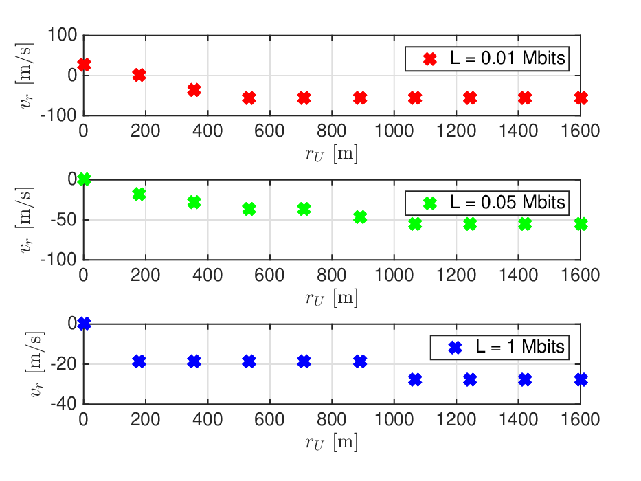
In Fig. 3, we depict the waiting phase policy, where the target average power constraint is fixed at $P_{\mathrm{avg}}{=}1000$ Watts, and the data payload value is varied for comparison. Note that for small data payload values, more consideration is placed on power minimization, hence the UAV seeks to move towards a positive radius value and move circularly at the power-minimizing speed until receiving a request; for larger data payloads, the minimization focuses more on communication delay, hence, the UAV seeks to reach the geometric center of the GNs quickly in order to position itself best in anticipation of future transmission requests.

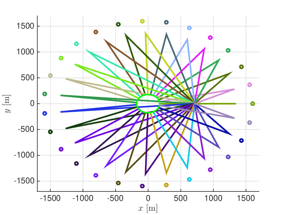
Next, we look at an example of the communication phase policy for a fixed data payload value of $L=1$Mbit, UAV position $(r_{U},\theta_{U}){=}(710,0)$m, request radius $r_{G}{=}1600$m, and varied relative request angles, $\theta_{G}$, as illustrated in Fig. 4. We observe the pattern of the relative distance between a requesting GN and the associated position $\mathbf{q}_{GU}$, where the UAV first receives $L$ bits from the GN. Additionally, a common end radius of $r_{UB}{=}178$m is found to be an optimal end point, even under variations in the relative request angles $\theta_{G}$.

Finally, in Fig. 5, we fix the data payload value at $L{=}1$Mbit and show how the optimal expected average delay, $\bar{D}_{\mu}^{*}$, changes for various target $P_{\mathrm{avg}}$ values in the range $[875,1850]$Watts. As expected, $\bar{D}_{\mu}^{*}$ decreases with increasing UAV power consumption. Additionally, the performance is compared to several other heuristics:

1. 1.

   Hover at center: The UAV always hovers at the center of the cell. The expected average delay is $90.59$[s], noticeably worse than the delay yielded by the optimal policy $\mu^{*}$ for any of the tested $P_{\mathrm{avg}}$ targets. Alternatively, if the GNs always transmit directly to the BS, we found that the performance is roughly the same, since the UAV-BS link incurs small delay thanks to the small UAV-BS distance.³³ 3 For this case, we use optimistically the same pathloss model as for the GN-UAV-BS links.

2. 2.

   Start-end at center: The UAV hovers at the center, awaiting requests; once a request is received, it moves at speed $v$ towards the GN at a certain radius $r_{GU}$, receives the $L$ bits from the GN, travels back at speed $v$ to the center, where it hovers to relay the data payload to the BS; $r_{GU}$ is optimized to minimize the communication delay of each request, whereas $v$ is varied so as to obtain different power consumptions. Note that the expected average communication delay is worse than the optimal policy $\mu^{*}$ across all values of $P_{\mathrm{avg}}$, except for smaller values of $P_{\mathrm{avg}}$ (due to the approximation introduced by discretization).

Overall, the optimal policy outperforms these heuristic schemes by a significant margin, hence demonstrating the importance of an adaptive design that optimizes the average long-term performance.

In this paper, we studied the trajectory optimization problem of one UAV acting as a relay in a two-phase, decode-and-forward strategy, servicing random uplink transmission requests by GNs seeking to communicate a data payload to a centralized BS. We formulated a continuous state and action space, discretized the problem into an SMDP, and solved it through dynamic programming. It was shown that the problem exhibits an interesting two-scale structure. Numerical evaluations demonstrate consistent improvements in the delay performance over sensible heuristics.

References

- [1] A. Fotouhi, H. Qiang, M. Ding, M. Hassan, L. G. Giordano, A. Garcia-Rodriguez, and J. Yuan, “Survey on uav cellular communications: Practical aspects, standardization advancements, regulation, and security challenges,” IEEE Communications Surveys Tutorials, pp. 1–1, 2019.
- [2] M. Mozaffari, W. Saad, M. Bennis, Y. Nam, and M. Debbah, “A tutorial on uavs for wireless networks: Applications, challenges, and open problems,” IEEE Communications Surveys Tutorials, pp. 1–1, 2019.
- [3] L. Gupta, R. Jain, and G. Vaszkun, “Survey of important issues in uav communication networks,” IEEE Communications Surveys Tutorials, vol. 18, no. 2, pp. 1123–1152, Secondquarter 2016.
- [4] Q. Wu, L. Liu, and R. Zhang, “Fundamental Trade-offs in Communication and Trajectory Design for UAV-Enabled Wireless Network,” IEEE Wireless Communications, vol. 26, pp. 36–44, 02 2019.
- [5] M. Bliss and N. Michelusi, “Trajectory optimization for rotary-wing uavs in wireless networks with random requests.” 2019. To appear at GLOBECOM 2019. https://arxiv.org/abs/1905.01755.
- [6] A. Fotouhi, M. Ding, and M. Hassan, “Dynamic base station repositioning to improve performance of drone small cells,” in 2016 IEEE Globecom Workshops (GC Wkshps), Dec 2016, pp. 1–6.
- [7] S. Chou, Y. Yu, and A. Pang, “Mobile small cell deployment for service time maximization over next-generation cellular networks,” IEEE Transactions on Vehicular Technology, vol. 66, no. 6, pp. 5398–5408, June 2017.
- [8] K. Li, W. Ni, X. Wang, R. P. Liu, S. S. Kanhere, and S. Jha, “Energy-efficient cooperative relaying for unmanned aerial vehicles,” IEEE Transactions on Mobile Computing, vol. 15, no. 6, pp. 1377–1386, June 2016.
- [9] Y. Zeng and R. Zhang, “Energy-efficient uav communication with trajectory optimization,” IEEE Transactions on Wireless Communications, vol. 16, no. 6, pp. 3747–3760, June 2017.
- [10] Y. Zeng, J. Xu, and R. Zhang, “Energy Minimization for Wireless Communication With Rotary-Wing UAV,” IEEE Transactions on Wireless Communications, vol. 18, no. 4, pp. 2329–2345, April 2019.
- [11] M.-H. Hwang, H.-R. Cha, and S. Jung, “Practical endurance estimation for minimizing energy consumption of multirotor unmanned aerial vehicles,” Energies, vol. 11, no. 9, 2018.
- [12] Y. Zeng, R. Zhang, and T. J. Lim, “Wireless communications with unmanned aerial vehicles: opportunities and challenges,” IEEE Communications Magazine, vol. 54, no. 5, pp. 36–42, May 2016.
- [13] J. D. C. Little and S. Graves, Little’s Law, 07 2008, pp. 81–100.