跳到论文正文
W Papers独立论文阅读器 arXiv:2002.09563 论文正文 计算阅读时间 · 0%
引用这篇论文根据当前论文元数据生成,正式投稿前建议核对。


License: arXiv.org perpetual non-exclusive license
arXiv:2002.09563v1 [math.NA] 19 Feb 2020

Structure-Preserving and Efficient Numerical Methods for Ion Transport

Jie Ding Thanks:  Department of Mathematics and Mathematical Center for Interdiscipline Research, Soochow University, 1 Shizi Street, Suzhou 215006, Jiangsu, China    Zhongming Wang Thanks:  Department of Mathematics and Statistics, Florida International University, Miami, FL, 33199, U. S. A.    Shenggao Zhou Thanks:  Corresponding author. Department of Mathematics and Mathematical Center for Interdiscipline Research, Soochow University, 1 Shizi Street, Suzhou 215006, Jiangsu, China. E-mail: sgzhou@suda.edu.cn.
Abstract

Ion transport, often described by the Poisson–Nernst–Planck (PNP) equations, is ubiquitous in electrochemical devices and many biological processes of significance. In this work, we develop conservative, positivity-preserving, energy dissipating, and implicit finite difference schemes for solving the multi-dimensional PNP equations with multiple ionic species. A central-differencing discretization based on harmonic-mean approximations is employed for the Nernst–Planck (NP) equations. The backward Euler discretization in time is employed to derive a fully implicit nonlinear system, which is efficiently solved by a newly proposed Newton’s method. The improved computational efficiency of the Newton’s method originates from the usage of the electrostatic potential as the iteration variable, rather than the unknowns of the nonlinear system that involves both the potential and concentration of multiple ionic species. Numerical analysis proves that the numerical schemes respect three desired analytical properties (conservation, positivity preserving, and energy dissipation) fully discretely. Based on advantages brought by the harmonic-mean approximations, we are able to establish estimate on the upper bound of condition numbers of coefficient matrices in linear systems that are solved iteratively. The solvability and stability of the linearized problem in the Newton’s method are rigorously established as well. Numerical tests are performed to confirm the anticipated numerical accuracy, computational efficiency, and structure-preserving properties of the developed schemes. Adaptive time stepping is implemented for further efficiency improvement. Finally, the proposed numerical approaches are applied to characterize ion transport subject to a sinusoidal applied potential.

AMS subject classifications: 65N06, 35K61, 35Q92, 92D15
Keywords: Ion transport; Harmonic-mean approximation; Conservation; Positivity; Energy dissipation; Newton’s method

1 Introduction

Ion transport plays a fundamental role in many applications, such as electrochemical energy devices [4], electrokinetics in microfluidics [48], and transmembrane ion channels [53]. It is often described by the so-called Poisson–Nernst–Planck (PNP) equations, which consist of the Poisson’s equation and the Nernst–Planck (NP) equations. Based on a mean-field approximation, the NP equations describe the diffusion of ions in the gradient of the electrostatic potential. The Poisson’s equation determines the electrostatic potential with the charge density arising from diffusing ions. Recently, there has been growing interests in incorporating effects that are beyond the mean-field description, e.g., the steric effect, inhomogeneous dielectric effect, and ion-ion correlations [26, 23, 37, 55, 24, 28, 39, 30, 46, 51, 25, 52, 45, 33, 49].

In this work, we develop efficient and structure-preserving finite difference schemes for the PNP equations

{∂tcl=∇⋅(∇cl+qlcl∇ψ),l=1,⋯,M,−κ​Δ​ψ=∑l=1Mql​cl+ρf.\left\{\begin{aligned} &\partial_{t}c^{l}=\nabla\cdot(\nabla c^{l}+q^{l}c^{l}\nabla\psi),~l=1,\cdots,M,\\ &-\kappa\Delta\psi=\sum_{l=1}^{M}q^{l}c^{l}+\rho^{f}.\end{aligned}\right. (1)

Here clc^{l} is the ion concentration for the ll-th species, qlq^{l} is the valence of the ll-th ionic species, κ>0\kappa>0 is a coefficient arising from nondimensionalization, ψ\psi is the electrostatic potential, and ρf\rho^{f} is the fixed charge density.

The analytical solutions to (1) with zero-flux boundary conditions possess several physically desired properties, including mass conservation, positivity preservation, and free-energy dissipation, i.e.,

∫Ωcl​(t,⋅)​𝑑V=∫Ωcinl​(⋅)​𝑑V,∀t>0,\displaystyle\int_{\Omega}c^{l}(t,\cdot)\,dV=\int_{\Omega}c^{l}_{\rm in}(\cdot)\,dV,\quad\forall t>0, (2a)
cinl​(⋅)>0⟹cl​(t,⋅)>0,∀t>0,\displaystyle c^{l}_{\rm in}(\cdot)>0\Longrightarrow c^{l}(t,\cdot)>0,\quad\forall t>0, (2b)
dd​tF=−∑l=1M∫Ω1cl(|∇cl+qlcl∇ψ|2)dV≤0,\displaystyle\frac{d}{dt}F=-\sum_{l=1}^{M}\int_{\Omega}\frac{1}{c^{l}}(|\nabla c^{l}+q^{l}c^{l}\nabla\psi|^{2})dV\leq 0, (2c)

where the free energy FF, aside from some boundary contributions, is defined by

F=∑l=1M∫Ω[cl​log⁡cl+12​(ql​cl+ρf)​ψ]​𝑑V.F=\sum_{l=1}^{M}\int_{\Omega}\left[c^{l}\log c^{l}+\frac{1}{2}(q^{l}c^{l}+\rho^{f})\psi\right]dV. (3)

The free energy contains both an entropic contribution and an electrostatic energy: cl​log​clc^{l}{\rm log}c^{l} is the entropy related to the Brownian motion of each ion species, and 12​(ql​cl+ρf)​ψ\frac{1}{2}(q^{l}c^{l}+\rho^{f})\psi is the (mean-field) electrostatic energy of the Coulomb interaction between charged ions. The concentrations are expected to converge to an equilibrium solution in a closed system regardless of how initial data are distributed.

These nice mathematical features are crucial for the analytical study of the PNP equations. For instance, by an energy estimate with the control of the free-energy dissipation, the solution is shown to converge to the thermal equilibrium state as time becomes large, if the boundary conditions are in thermal equilibrium (see, e.g., [16]). Long time behavior was studied in [6], and further in [2, 5] with refined convergence rates. Results for the drift-diffusion model, i.e., the PNP equations in the semiconductor literature, with regarding global existence, uniqueness, and asymptotic behavior in the case of different boundary conditions have been established in the works [42, 17, 13, 12].

The PNP equations can hardly be solved analytically due to the nonlinear coupling of the electrostatic potential and ionic concentrations. Much effort has been devoted to the development of numerical methods in various applications [7, 43, 36, 54, 15, 8, 31, 41, 35, 50, 40, 14, 18, 32, 9, 49, 44, 10]. The existing algorithms range from finite difference to finite elements in both one dimension and high dimensions. Among these developed schemes, several attempts are made to design desirable numerical schemes that respect the nice properties (2) of analytical solutions. In [15], for instance, a second-order conservative, energy dissipative finite difference method was presented for the one-dimensional PNP equations. A delicate temporal discretization scheme was designed to preserve energy dynamics in [14]. A hybrid conservative scheme that uses adaptive grids was developed to solve the PNP equations on irregular domains [41]. A type of finite difference schemes has been developed using the Slotboom transformation of the Nernst–Planck (NP) equations:

∂tcl=∇⋅(e−ql​ψ∇gl),\partial_{t}c^{l}=\nabla\cdot\left(e^{-q^{l}\psi}\nabla g^{l}\right), (4)

where gl=cl​eql​ψg^{l}=c^{l}e^{q^{l}\psi} are the Slotboom variables [38, 36, 39, 32, 33]. By using the Slotboom variables, Liu and Wang [31] developed a free energy satisfying finite difference scheme that preserves those three properties with rigorous proof in one dimension. A free energy satisfying discontinuous Galerkin method was also developed by the same authors in [32], in which the positivity of numerical solutions was not proved but enforced by an accuracy-preserving limiter. An implicit finite difference scheme was developed to solve the PNP equations with properties of positivity preservation and energy dissipation [22]. The resulting nonlinear discretization system was numerically solved by a fixed-point iteration method. Gao and He [18] proposed a linearized convergent finite element scheme that conserves total concentration and preserves the electric energy. Rigorous error analysis of finite element type methods for the PNP equations has been studied in [50, 19]. A finite element discretization that can enforce positivity of numerical solutions was developed for the PNP equations, as well as the PNP equations coupling with the incompressible Navier-Stokes equations [40].

Although some progress has been made on the development of numerical methods that ensure the desired properties, it is still desirable to have computationally efficient and robust finite difference schemes that incorporate all three desired properties together, especially in high dimensions. Among three properties (2), the preservation of positivity is crucial to the validity of a numerical solution and is in particular hard to achieve. For instance, the positivity has been proved in [15] for the one-dimensional PNP equations, under assumptions that the gradient of the electrostatic potential is bounded and mesh step sizes satisfy certain constraint conditions. The numerical scheme developed in [31] has been proved to preserve positivity of the numerical solution but in one-dimensional case. Furthermore, one constraint on a mesh ratio needs to be satisfied to ensure positivity, due to the explicit nature of the scheme. From a practical point of view, implicit or semi-implicit schemes that preserve positivity are much more computationally efficient, because larger time-stepping sizes are allowed in temporal integration. In our recent work [11], we proposed efficient semi-implicit schemes that respect the desired properties. While the scheme allows relatively large time steps and is successful in positivity persevering and mass conservation, the energy dissipation is only proved in a semi-discrete form.

In this work, we develop implicit finite difference schemes for the multi-dimensional PNP equations with multiple ionic species that respect conservation, positivity preserving, and energy dissipation at fully discrete level. The NP equations reformulated in the Slotboom variables are spatially discretized by a central-differencing scheme based on harmonic-mean approximations. The backward Euler method in time is employed to derive a nonlinear coupled system, which is efficiently solved by a newly proposed Newton’s method. The improved efficiency of the Newton’s method is achieved via using the electrostatic potential as the iteration variable, rather than the unknowns of the nonlinear system that involves both the potential and concentrations of multiple ionic species. The advantages of the proposed Newton’s method in saving memory and computational efficiency become more significant when the number of ionic species gets larger. In addition, numerical simulations demonstrate that the Newton’s method requires appreciably fewer iteration steps and less computational time, in comparison with a typical fixed-point iteration method. Such a Netwon’s method can be employed to solve nonlinear systems resulting from other implicit discretization of the PNP-type equations.

We perform detailed numerical analysis to prove that the numerical schemes respect three desired analytical properties fully discretely. Thanks to the advantages brought by the harmonic-mean approximations, we are able to establish upper bounds on condition numbers of coefficient matrices of linear systems resulting from both the discretization of the NP equations, and solvability and stability of the linearized problem in the Newton’s method. The linear systems are efficiently solved using iterative methods with preconditioners. Numerical simulations are presented to demonstrate that the developed schemes have expected numerical accuracy, computational efficiency, and structure-preserving properties. An adaptive time stepping strategy is employed to achieve further improvement in computational efficiency. The benefit of the adaptive time stepping is demonstrated in the application of the proposed numerical approaches to probing ion transport in response to an alternating applied potential. Finally, the developed numerical approaches are applied to understand charge dynamics in electrolytes between two parallel electrodes exposed to sinusoidal applied potentials. The impact of frequency of the sinusoidal applied potentials is extensively investigated in numerical simulations.

The rest of this paper is organized as follows. In Section §3, we start with details of our settings, and present our implicit finite difference method in both spatial and temporal discretization. In Section §4 we prove the main properties at fully discrete level, including conservation, free-energy dissipation, positivity preservation. Section §5 is devoted to numerical examples, including accuracy test, charge dynamics, and adaptive time stepping. Finally, we conclude in Section §6.

2 The PNP equations

We consider the initial-boundary value problem

{∂tcl=∇⋅(∇cl+qlcl∇ψ) for t>0 and l=1,⋯,M,−κ​Δ​ψ=∑l=1Mql​cl+ρf,cl​(0,⋅)=cinl​(⋅),∂cl∂n+ql​cl​∂ψ∂n=0​ on ​∂Ω,ψ(⋅)=V(⋅) on ΓD, and κ∂ψ∂n=σ(⋅) on ΓN.\left\{\begin{aligned} &\partial_{t}c^{l}=\nabla\cdot(\nabla c^{l}+q^{l}c^{l}\nabla\psi)\mbox{~~for~}t>0\mbox{~and~}l=1,\cdots,M,\\ &-\kappa\Delta\psi=\sum_{l=1}^{M}q^{l}c^{l}+\rho^{f},\\ &c^{l}(0,\cdot)=c^{l}_{\rm in}(\cdot),\\ &\frac{\partial c^{l}}{\partial\textbf{n}}+q^{l}c^{l}\frac{\partial\psi}{\partial\textbf{n}}=0\mbox{~~on~}\partial\Omega,\\ &\psi(\cdot)=V(\cdot)\mbox{~~on~}\Gamma_{D},\mbox{~~and~}\kappa\frac{\partial\psi}{\partial\textbf{n}}=\sigma(\cdot)\mbox{~~on~}\Gamma_{N}.\end{aligned}\right. (5)

Here Ω\Omega is a bounded domain, n is a unit exterior normal vector on the boundary ∂Ω\partial\Omega, cinlc^{l}_{\rm in} are initial concentration distributions. To be general, we here consider both Dirichlet and Neumann boundary conditions for the electrostatic potential, i.e., V⁡(x)V(x) is a given electrostatic potential defined on the Dirichlet boundary ΓD\Gamma_{D}, and σ⁡(x)\sigma(x) is the surface charge density defined on the Neumann boundary ΓN\Gamma_{N} with ΓD∩ΓN=Ø\Gamma_{D}\cap\Gamma_{N}=\O and ΓD∪ΓN=∂Ω\Gamma_{D}\cup\Gamma_{N}=\partial\Omega. The corresponding total free energy with boundary contributions is given by [34]

F=∑l=1M∫Ω[cl​log⁡cl+12​(ql​cl+ρf)​ψ]​𝑑V−12​∫ΓDκ​∂ψ∂𝐧​V​𝑑S+12​∫ΓNσ​ψ​𝑑S.F=\sum_{l=1}^{M}\int_{\Omega}\left[c^{l}\log c^{l}+\frac{1}{2}(q^{l}c^{l}+\rho^{f})\psi\right]dV-\frac{1}{2}\int_{\Gamma_{D}}\kappa\frac{\partial\psi}{\partial{\bf n}}VdS+\frac{1}{2}\int_{\Gamma_{N}}\sigma\psi dS. (6)

With initial-boundary conditions given in (5), the property of free-energy dissipation (2c) can be derived as well.

Theorem 2.1

The solution to the PNP equations (5) satisfies the energy dissipation law

d​Fd​t=−∑l=1M∫Ω1cl|∇cl+qlcl∇ψ|2dV+∫ΓNd​σd​tψdS−∫ΓDκ∂ψ∂𝐧d​Vd​tdS.\displaystyle\frac{dF}{dt}=-\sum_{l=1}^{M}\int_{\Omega}\frac{1}{c^{l}}|\nabla c^{l}+q^{l}c^{l}\nabla\psi|^{2}dV+\int_{\Gamma_{N}}\frac{d\sigma}{dt}\psi dS-\int_{\Gamma_{D}}\kappa\frac{\partial\psi}{\partial{\bf n}}\frac{dV}{dt}dS. (7)

Taking a derivative with respect to time, we have by integration by parts that

dd​t​F=\displaystyle\frac{d}{dt}F= −∫Ω∑Ml=11cl|∇c+qlcl∇ψ|2+12((qlcl+ρf)d​ψd​t−qld​cld​tψ)dV\displaystyle-\int_{\Omega}\sum^{M}_{l=1}\frac{1}{c^{l}}|\nabla c+q^{l}c^{l}\nabla\psi|^{2}+\frac{1}{2}\left((q^{l}c^{l}+\rho^{f})\frac{d\psi}{dt}-q^{l}\frac{dc^{l}}{dt}\psi\right)\,dV
+12∫ΓN[d​σd​tψ+σd​ψd​t]dS−12∫ΓDκ[dd​t(∂ψ∂𝐧)V+∂ψ∂𝐧d​Vd​t]dS.\displaystyle+\frac{1}{2}\int_{\Gamma_{N}}\left[\frac{d\sigma}{dt}\psi+\sigma\frac{d\psi}{dt}\right]\,dS-\frac{1}{2}\int_{\Gamma_{D}}\kappa\left[\frac{d}{dt}\left(\frac{\partial\psi}{\partial\mathbf{n}}\right)V+\frac{\partial\psi}{\partial\mathbf{n}}\frac{dV}{dt}\right]\,dS.

It follows from the Poisson’s equation that

∑l=1M12​∫Ω((ql​cl+ρf)​d​ψd​t−ql​d​cld​t​ψ)​𝑑V\displaystyle\sum_{l=1}^{M}\frac{1}{2}\int_{\Omega}\left((q^{l}c^{l}+\rho^{f})\frac{d\psi}{dt}-q^{l}\frac{dc^{l}}{dt}\psi\right)\,dV
=12​∫ΓN[ψ​d​σd​t−σ​d​ψd​t]​𝑑S+12​∫ΓDκ⁡[dd​t​(∂ψ∂𝐧)​V−∂ψ∂𝐧​d​Vd​t]​𝑑S\displaystyle=\frac{1}{2}\int_{\Gamma_{N}}\left[\psi\frac{d\sigma}{dt}-\sigma\frac{d\psi}{dt}\right]\,dS+\frac{1}{2}\int_{\Gamma_{D}}\kappa\left[\frac{d}{dt}\left(\frac{\partial\psi}{\partial\mathbf{n}}\right)V-\frac{\partial\psi}{\partial\mathbf{n}}\frac{dV}{dt}\right]\,dS

Substituting into the above equation completes the proof.    One can observe from (7) that the total free energy of the system is dissipating if the boundary data are independent of time.

3 Numerical Method

3.1 Discretization and Notations

The spatial discretization is similar to our previous work [11]. For completeness of the presentation, we briefly introduce notations and recall the discretization scheme. For simplicity, we consider a 2D rectangular computational domain Ω=[a,b]×[c,d]\Omega=[a,b]\times[c,d] with boundaries

ΓD={(x,y):x=aorb,c≤y≤d}and ΓN={(x,y):y=cord,a≤x≤b}.\Gamma_{D}=\left\{(x,y):x=a~\text{or}~b,~c\leq y\leq d\right\}~\text{and }\Gamma_{N}=\left\{(x,y):y=c~\text{or}~d,~a\leq x\leq b\right\}.

The computational domain is covered by the non-uniform grid points {xi,yj}\left\{x_{i},y_{j}\right\} with

a=x12<x32<⋯<xNx+12=b,\displaystyle a=x_{\frac{1}{2}}<x_{\frac{3}{2}}<\dots<x_{N_{x}+\frac{1}{2}}=b,
c=y12<y32<⋯<yNy+12=d,\displaystyle c=y_{\frac{1}{2}}<y_{\frac{3}{2}}<\dots<y_{N_{y}+\frac{1}{2}}=d,

where NxN_{x} and NyN_{y} are the number of grid points along each dimension. We also introduce grid points with integer indices:

xi=xi−12+xi+122andyj=yj−12+yj+122for ​i=1,…,Nx,j=1,…,Ny.x_{i}=\frac{x_{i-\frac{1}{2}}+x_{i+\frac{1}{2}}}{2}\quad\text{and}\quad y_{j}=\frac{y_{j-\frac{1}{2}}+y_{j+\frac{1}{2}}}{2}~~~~\text{for }i=1,\dots,N_{x},~j=1,\dots,N_{y}.

The grid spacings are given by

hxi=xi+12−xi−12,hyj=yj+12−yj−12for i=1,…,Nx,j=1,…,Ny,h^{x}_{i}=x_{i+\frac{1}{2}}-x_{i-\frac{1}{2}},~h^{y}_{j}=y_{j+\frac{1}{2}}-y_{j-\frac{1}{2}}~\text{for }i=1,\dots,N_{x},~j=1,\dots,N_{y},

and

hxi+12=xi+1−xi,hyj+12=yj+1−yjfor i=1,…,Nx−1,j=1,…,Ny−1.h^{x}_{i+\frac{1}{2}}=x_{i+1}-x_{i},~h^{y}_{j+\frac{1}{2}}=y_{j+1}-y_{j}~\text{for }i=1,\dots,N_{x}-1,~j=1,\dots,N_{y}-1.

We denote by ci,jlc^{l}_{i,j}, gi,jlg^{l}_{i,j}, and ψi,j\psi_{i,j} the semi-discrete approximations of cl​(t,xi,yj)c^{l}(t,x_{i},y_{j}), gl​(t,xi,yj)g^{l}(t,x_{i},y_{j}), and ψ⁡(t,xi,yj)\psi(t,x_{i},y_{j}), respectively. Define discrete operators

Dx+fi,j=fi+1,j−fi,jhi+12x,D2xfi,j=Dx+​fi,j−Dx+​fi−1,jhix.\displaystyle D_{x}^{+}f_{i,j}=\frac{f_{i+1,j}-f_{i,j}}{h^{x}_{i+\frac{1}{2}}},\quad D^{2}_{x}f_{i,j}=\frac{D_{x}^{+}f_{i,j}-D_{x}^{+}f_{i-1,j}}{h^{x}_{i}}.

Discrete operators Dy+D_{y}^{+} and Dy2D^{2}_{y} can be analogously defined. Also, we introduce

hxm=min(hx1,⋯,hxNx),hxM=max(hx1,⋯,hxNx),\displaystyle h^{x}_{m}=\min(h^{x}_{1},\cdots,h^{x}_{N_{x}}),~h^{x}_{M}=\max(h^{x}_{1},\cdots,h^{x}_{N_{x}}),
hym=min(hy1,⋯,hyNy),hyM=max(hy1,⋯,hyNy).\displaystyle h^{y}_{m}=\min(h^{y}_{1},\cdots,h^{y}_{N_{y}}),~h^{y}_{M}=\max(h^{y}_{1},\cdots,h^{y}_{N_{y}}).

We now present our implicit finite difference method by discretiztion in space and time separately. Note that, although our discretization is presented for a 2D case, it can be readily extended to three dimensions in a dimension-by-dimension manner.

3.2 Finite difference method in space

1) Spatial discretization of the Poisson’s equation

With given semi-discrete approximations ci,jlc^{l}_{i,j}, we discretize the Poisson’s equation with a central differencing stencil

−κ(Dx2+Dy2)ψi,j=∑l=1Mqlci,jl+ρi,jf,i=1,…,Nx,j=1,…,Ny.-\kappa(D^{2}_{x}+D^{2}_{y})\psi_{i,j}=\sum_{l=1}^{M}q^{l}c^{l}_{i,j}+\rho^{f}_{i,j},~i=1,\dots,N_{x},~j=1,\dots,N_{y}. (8)

We employ central differencing stencils again to discretize the Dirichlet boundary conditions on ΓD\Gamma_{D} by

ψ0,j+ψ1,j2=ψD(t,a,yj),ψNx+1,j+ψNx,j2=ψD(t,b,yj)forj=1,…,Ny,\displaystyle\frac{\psi_{0,j}+\psi_{1,j}}{2}=\psi_{D}(t,a,y_{j}),\quad\frac{\psi_{N_{x}+1,j}+\psi_{N_{x},j}}{2}=\psi_{D}(t,b,y_{j})~~\mbox{for}~~j=1,\dots,N_{y}, (9)

and the Neumann boundary conditions on ΓN\Gamma_{N} by

−κ​Dy+​ψi,0\displaystyle-\kappa D_{y}^{+}\psi_{i,0} =σ(t,xi,a),κDy+ψi,Ny=σ(t,xi,b)fori=1,…,Nx.\displaystyle=\sigma({t,x_{i},a}),\quad\kappa D_{y}^{+}\psi_{i,N_{y}}=\sigma({t,x_{i},b})~~\mbox{for}~~i=1,\dots,N_{x}. (10)

Notice that the definition of the boundary data ψD\psi_{D} and σ\sigma have been extended to the whole computational domain. In numerical implementation, the ghost points outside Ω\Omega are eliminated by coupling the discretization scheme (8) and boundary discretization (9) and (10). The coupled difference equations can be written in a matrix form

ℒ​𝝍=∑l=1Mql​𝒄l+𝝆f+𝒃.\mathcal{L}\boldsymbol{\psi}=\sum_{l=1}^{M}q^{l}\boldsymbol{c}^{l}+\boldsymbol{\rho}^{f}+\boldsymbol{b}. (11)

Here ℒ\mathcal{L} is the coefficient matrix, the column vector 𝒃\boldsymbol{b} results from the boundary conditions (9) and (10), and 𝝍\boldsymbol{\psi}, 𝒄l\boldsymbol{c}^{l}, and 𝝆f\boldsymbol{\rho}^{f} are vectors with components being ψi,j\psi_{i,j}, ci,jlc^{l}_{i,j}, and ρi,jf\rho^{f}_{i,j}, respectively.

2) Spatial discretization of the NP equations

We first introduce a Slotboom reformulation of the Nernst–Planck equations:

∂tcl=∇⋅(e−Sl∇gl),\partial_{t}c^{l}=\nabla\cdot\left(e^{-S^{l}}\nabla g^{l}\right), (12)

where Sl=ql​ψS^{l}=q^{l}\psi and gl=cl​eSlg^{l}=c^{l}e^{S^{l}}, which are the Slotboom variables [36, 32].

It follows from central-differencing discretization of Eq. (12) at {xi,yj}\{x_{i},y_{j}\} that

hix​hjy​dd​t​ci,jl=\displaystyle h^{x}_{i}h^{y}_{j}\frac{d}{dt}c^{l}_{i,j}= hjy​(e−Si+12,jl​g^x,i+12,jl−e−Si−12,jl​g^x,i−12,jl)\displaystyle h^{y}_{j}\left(e^{-S^{l}_{i+\frac{1}{2},j}}\widehat{g}_{x,i+\frac{1}{2},j}^{l}-e^{-S^{l}_{i-\frac{1}{2},j}}\widehat{g}_{x,i-\frac{1}{2},j}^{l}\right) (13)
+hix​(e−Si,j+12l​g^y,i,j+12l−e−Si,j−12l​g^y,i,j−12l):=Qi,j​(cl,Sl),\displaystyle+h^{x}_{i}\left(e^{-S^{l}_{i,j+\frac{1}{2}}}\widehat{g}_{y,i,j+\frac{1}{2}}^{l}-e^{-S^{l}_{i,j-\frac{1}{2}}}\widehat{g}_{y,i,j-\frac{1}{2}}^{l}\right):=Q_{i,j}(c^{l},S^{l}),

where the flux is approximated by

g^x,i+12,jl=ci+1,jl​eSi+1,jl−ci,jl​eSi,jlhi+12x​and ​g^y,i,j+12l=ci,j+1l​eSi,j+1l−ci,jl​eSi,jlhj+12y.\widehat{g}^{l}_{x,i+\frac{1}{2},j}=\frac{c_{i+1,j}^{l}e^{S^{l}_{i+1,j}}-c_{i,j}^{l}e^{S^{l}_{i,j}}}{h^{x}_{i+\frac{1}{2}}}~\text{and }~\widehat{g}^{l}_{y,i,j+\frac{1}{2}}=\frac{c_{i,j+1}^{l}e^{S^{l}_{i,j+1}}-c_{i,j}^{l}e^{S^{l}_{i,j}}}{h^{y}_{j+\frac{1}{2}}}. (14)

Harmonic-mean approximations are proposed in [11] to approximate the exponential terms at half-grid points:

e−Si+12,jl=2​e−Si+1,jl​e−Si,jle−Si+1,jl+e−Si,jl​and ​e−Si,j+12l=2​e−Si,j+1l​e−Si,jle−Si,j+1l+e−Si,jl.\displaystyle e^{-S^{l}_{i+{\frac{1}{2}},j}}=\frac{2e^{-S^{l}_{i+1,j}}e^{-S^{l}_{i,j}}}{e^{-S^{l}_{i+1,j}}+e^{-S^{l}_{i,j}}}~\text{and }~e^{-S^{l}_{i,j+{\frac{1}{2}}}}=\frac{2e^{-S^{l}_{i,j+1}}e^{-S^{l}_{i,j}}}{e^{-S^{l}_{i,j+1}}+e^{-S^{l}_{i,j}}}. (15)

The zero-flux boundary conditions are discretized by

g^lx,12,j=0,g^lx,Nx+12,j=0,j=1,…,Ny,\displaystyle\widehat{g}^{l}_{x,\frac{1}{2},j}=0,\quad\widehat{g}^{l}_{x,N_{x}+\frac{1}{2},j}=0,~~j=1,\dots,N_{y}, (16)
g^ly,i,12=0,g^ly,i,Ny+12=0,i=1,…,Nx.\displaystyle\widehat{g}^{l}_{y,i,\frac{1}{2}}=0,\quad\widehat{g}^{l}_{y,i,N_{y}+\frac{1}{2}}=0,~~i=1,\dots,N_{x}.

3.3 Backward Euler method in time

To obtain numerical solutions of concentrations at different time steps, the semi-discrete scheme can be integrated with various ODE solvers implicitly. With a nonuniform time step size Δ​tn\Delta t^{n} and tn=tn−1+Δ​tnt_{n}=t_{n-1}+\Delta t^{n}, ci,jl,nc^{l,n}_{i,j}, gi,jl,ng^{l,n}_{i,j}, and Si,jl,nS^{l,n}_{i,j} are used to denote the numerical approximations of cl​(tn,xi,yj)c^{l}(t_{n},x_{i},y_{j}), gl​(tn,xi,yj)g^{l}(t_{n},x_{i},y_{j}), and Sl​(tn,xi,yj)S^{l}(t_{n},x_{i},y_{j}), respectively.

We employ the backward Euler discretization in clc^{l}:

ci,jl,n+1−ci,jl,nΔ​tn+1=Qi,j​(cl,n+1,Sl,n+1),\frac{c_{i,j}^{l,n+1}-c_{i,j}^{l,n}}{\Delta t^{n+1}}=Q_{i,j}(c^{l,n+1},S^{l,n+1}), (17)

which gives a fully implicit nonlinear system. Note that the zero-flux boundary conditions (16) have been used in (17). We further rewrite (17) in a matrix form as

𝒜l(𝝍n+1)𝒄l,n+1=𝒫𝒄l,n,l=1,⋯,M.\mathcal{A}^{l}(\boldsymbol{\psi}^{n+1})\boldsymbol{c}^{l,n+1}=\mathcal{P}\boldsymbol{c}^{l,n},~l=1,\cdots,M. (18)

Here 𝒜l​(𝝍n+1)\mathcal{A}^{l}(\boldsymbol{\psi}^{n+1}) is a square matrix dependent on qlq^{l} and 𝝍n+1\boldsymbol{\psi}^{n+1}, 𝒫\mathcal{P} is a diagonal matrix given by

𝒫=diag​(h1x​h1y,⋯,h1x​hNyy,h2x​h1y,⋯,h2x​hNyy,⋯,hNxx​h1y,⋯,hNxx​hNyy),\mathcal{P}=\text{diag}\left(h^{x}_{1}h^{y}_{1},\cdots,h^{x}_{1}h^{y}_{N_{y}},h^{x}_{2}h^{y}_{1},\cdots,h^{x}_{2}h^{y}_{N_{y}},\cdots,h^{x}_{N_{x}}h^{y}_{1},\cdots,h^{x}_{N_{x}}h^{y}_{N_{y}}\right),

and 𝒄l,n+1\boldsymbol{c}^{l,n+1} and 𝒄l,n\boldsymbol{c}^{l,n} are column vectors with components being ci,jl,n+1c^{l,n+1}_{i,j} and ci,jl,nc^{l,n}_{i,j}, respectively.

An adaptive time stepping strategy is often useful in speeding up simulations of charged systems that have time-dependent boundary input data. One efficient way to adjust the time step sizes has been proposed in [47, 29]:

Δ​tn+1=max⁡(Δ​tmin,Δ​tmax1+α​|F′​(t)|2),\Delta t^{n+1}=\max\left(\Delta t_{\rm min},\frac{\Delta t_{\rm max}}{\sqrt{1+\alpha|F^{\prime}(t)|^{2}}}\right), (19)

where α\alpha is a given constant, F⁡(t)F(t) is the free energy defined by (6). In our numerical implementation, the temporal derivative of the free energy is approximated by a difference quotient. The time steps Δ​tmin\Delta t_{\rm min} and Δ​tmax\Delta t_{\rm max} dictate the lower and upper bounds of the adaptive time steps, respectively, i.e., Δ​tmin≤Δ​tn+1≤Δ​tmax\Delta t_{\rm min}\leq\Delta t^{n+1}\leq\Delta t_{\rm max}.

4 Properties of numerical solutions

The numerical solution has several important properties, as stated in the following theorems.

Theorem 4.1

(Mass conservation)The fully implicit scheme (17) respect conservation of concentration, in the sense that the total concentration remains constant in time, i.e.,

dd​t​∑i=1Nx∑j=1Nyci,jl​hix​hjy=0,\displaystyle\frac{d}{dt}\sum_{i=1}^{N_{x}}\sum_{j=1}^{N_{y}}c_{i,j}^{l}h^{x}_{i}h^{y}_{j}=0, (20)
∑i=1Nx∑j=1Nyci,jl,n+1​hix​hjy=∑i=1Nx∑j=1Nyci,jl,n​hix​hjy.\displaystyle\sum_{i=1}^{N_{x}}\sum_{j=1}^{N_{y}}c_{i,j}^{l,n+1}h^{x}_{i}h^{y}_{j}=\sum_{i=1}^{N_{x}}\sum_{j=1}^{N_{y}}c_{i,j}^{l,n}h^{x}_{i}h^{y}_{j}. (21)

It follows from (13) that

dd​t​∑i=1Nx∑j=1Nyci,jl​hix​hjy\displaystyle\frac{d}{dt}\sum_{i=1}^{N_{x}}\sum_{j=1}^{N_{y}}c^{l}_{i,j}h^{x}_{i}h^{y}_{j} =∑j=1Nyhjy​(e−SNx+12,jl​g^x,Nx+12l−e−S12,jl​g^x,12l)\displaystyle=\sum_{j=1}^{N_{y}}h^{y}_{j}\left(e^{-S^{l}_{N_{x}+\frac{1}{2},j}}\widehat{g}_{x,N_{x}+\frac{1}{2}}^{l}-e^{-S^{l}_{\frac{1}{2},j}}\widehat{g}_{x,\frac{1}{2}}^{l}\right)
+∑i=1Nxhix(e−Si,Ny+12lg^y,Ny+12l−e−Si,12lg^y,12l)=0,\displaystyle\quad+\sum_{i=1}^{N_{x}}h^{x}_{i}\left(e^{-S^{l}_{i,N_{y}+\frac{1}{2}}}\widehat{g}_{y,N_{y}+\frac{1}{2}}^{l}-e^{-S^{l}_{i,\frac{1}{2}}}\widehat{g}_{y,\frac{1}{2}}^{l}\right)=0,

where we have used the zero-flux boundary conditions (16) in the last step. Similarly, summing both sides of (17) over i,ji,j gives

∑i=1Nx∑j=1Nyci,jl,n+1​hix​hjy−∑i=1Nx∑j=1Nyci,jl,n​hix​hjy=Δ​tn+1​∑i=1Nx∑j=1NyQi,j​(cl,n+1,Sl,n+1)​hix​hjy.\sum_{i=1}^{N_{x}}\sum_{j=1}^{N_{y}}c_{i,j}^{l,n+1}h^{x}_{i}h^{y}_{j}-\sum_{i=1}^{N_{x}}\sum_{j=1}^{N_{y}}c_{i,j}^{l,n}h^{x}_{i}h^{y}_{j}=\Delta t^{n+1}\sum_{i=1}^{N_{x}}\sum_{j=1}^{N_{y}}Q_{i,j}(c^{l,n+1},S^{l,n+1})h^{x}_{i}h^{y}_{j}.

Incorporating the zero-flux boundary conditions (16) at time tn+1t_{n+1} for gl,n+1=cl,n+1​eSn+1g^{l,n+1}=c^{l,n+1}e^{S^{n+1}} leads to (21).    

Theorem 4.2

(Positivity preserving)The numerical solutions ci,jl,n+1c_{i,j}^{l,n+1} computed from the backward Euler scheme (17) remain positive in time, i.e., if ci,jl,n>0c_{i,j}^{l,n}>0, then

ci,jl,n+1>0​ for ​i=1,⋯,Nx,j=1,⋯,Ny.c_{i,j}^{l,n+1}>0~\text{ for }i=1,\cdots,N_{x},~j=1,\cdots,N_{y}.

Analogous to the derivation in our previous work [11], we can show that

{∑i=1Nx​Ny𝒜i,jl=hix​hjyfor​j=1,…,Nx​Ny,1<𝒜i,il<1+4​Δ​tn+1​(hMxhmy+hMyhmx)for​i=1,…,Nx​Ny,−2​max⁡{hMxhmy,hMyhmx}<𝒜i,jl≤0for​i,j=1,…,Nx​Ny,and​i≠j.\left\{\begin{aligned} &\sum_{i=1}^{N_{x}N_{y}}\mathcal{A}^{l}_{i,j}=h^{x}_{i}h^{y}_{j}\quad\mbox{for}~j=1,\dots,N_{x}N_{y},\\ &1<\mathcal{A}^{l}_{i,i}<1+4\Delta t^{n+1}(\frac{h^{x}_{M}}{h^{y}_{m}}+\frac{h^{y}_{M}}{h^{x}_{m}})\qquad\quad\mbox{for}~i=1,\dots,N_{x}N_{y},\\ &-2\max\{\frac{h^{x}_{M}}{h^{y}_{m}},\frac{h^{y}_{M}}{h^{x}_{m}}\}<\mathcal{A}^{l}_{i,j}\leq 0\qquad\quad\mbox{for}~i,j=1,\dots,N_{x}N_{y},~\mbox{and}~i\neq j.\end{aligned}\right. (22)

We can verify that 𝒜l\mathcal{A}^{l} is an M-matrix and 𝒜l,−1>0\mathcal{A}^{l,-1}>0 in the element-wise sense. Thus, ci,jl,n+1>0c_{i,j}^{l,n+1}>0 if ci,jl,n>0c_{i,j}^{l,n}>0.   

The concentrations are obtained by solving the linear system (18) iteratively. For iterative methods, it is desirable to establish estimates on the condition number of the coefficient matrix. We now recall the estimate on the condition number of the coefficient matrix 𝒜l\mathcal{A}^{l} in the work [11], and brief the corresponding proof with minor modifications.

Theorem 4.3

The condition number of the coefficient matrix 𝒜l\mathcal{A}^{l} satisfies

κ1​(𝒜l):=‖𝒜l‖1​‖𝒜l,−1‖1≤hMx​hMyhmx​hmy+8​Δ​tn+1​[hMy(hmx)2​hmy+hMxhmx​(hmy)2].\kappa_{1}(\mathcal{A}^{l}):=\|\mathcal{A}^{l}\|_{1}\|\mathcal{A}^{l,-1}\|_{1}\leq\frac{h^{x}_{M}h^{y}_{M}}{h^{x}_{m}h^{y}_{m}}+8\Delta t^{n+1}\left[\frac{h^{y}_{M}}{(h^{x}_{m})^{2}h^{y}_{m}}+\frac{h^{x}_{M}}{h^{x}_{m}(h^{y}_{m})^{2}}\right]. (23)

From the proof of Theorem 4.2, we know that 𝒜l\mathcal{A}^{l} is an M-matrix, and therefore 𝒜l,−1\mathcal{A}^{l,-1} exists and is a non-negative matrix. As shown in [11], we can further prove that

hmx​hmy​ν​𝒜l,−1≤ν,h^{x}_{m}h^{y}_{m}\nu\mathcal{A}^{l,-1}\leq\nu,

where ν=(1,⋯,1⏟Nx​Ny)\nu=(\underbrace{1,\cdots,1}_{N_{x}N_{y}}). This implies that each column sum of (𝒜l)−1(\mathcal{A}^{l})^{-1} is less or equal to 1hmx​hmy\frac{1}{h^{x}_{m}h^{y}_{m}}. Since each element in (𝒜l)−1(\mathcal{A}^{l})^{-1} is non-negative, we obtain ‖(𝒜l)−1‖1≤1hmx​hmy\|(\mathcal{A}^{l})^{-1}\|_{1}\leq\frac{1}{h^{x}_{m}h^{y}_{m}}. Also, it follows from (22) that

‖𝒜l‖1≤hMx​hMy+8​Δ​tn+1​(hMyhmx+hMxhmy).\|\mathcal{A}^{l}\|_{1}\leq h^{x}_{M}h^{y}_{M}+8\Delta t^{n+1}\left(\frac{h^{y}_{M}}{h^{x}_{m}}+\frac{h^{x}_{M}}{h^{y}_{m}}\right).

This completes the proof by the definition of the 11-norm condition number.    

Our numerical scheme also respects the property of free-energy dissipation at full discrete level, when the boundary data is independent of time. The total discrete free energy (6) is approximated by

Fhn=\displaystyle F^{n}_{h}= ∑l=1M∑i=1Nx∑j=1Nyhix​hjy​[ci,jl,n​log⁡ci,jl,n+12​(ql​ci,jl,n+ρi,jf)​ψi,jn]\displaystyle\sum_{l=1}^{M}\sum_{i=1}^{N_{x}}\sum_{j=1}^{N_{y}}h^{x}_{i}h^{y}_{j}\left[c^{l,n}_{i,j}\log c^{l,n}_{i,j}+\frac{1}{2}(q^{l}c^{l,n}_{i,j}+\rho^{f}_{i,j})\psi^{n}_{i,j}\right] (24)
−∑j=1Nyhyjκ[VNx+12,j(VNx+12,j−ψNx,jn)hix+V12,j(V12,j−ψ1,jn)hix]\displaystyle-\sum_{j=1}^{N_{y}}h^{y}_{j}\kappa\left[V_{N_{x}+\frac{1}{2},j}\frac{(V_{N_{x}+\frac{1}{2},j}-\psi^{n}_{N_{x},j})}{h^{x}_{i}}+V_{\frac{1}{2},j}\frac{(V_{\frac{1}{2},j}-\psi^{n}_{1,j})}{h^{x}_{i}}\right]
+∑i=1Nxhix2[σi,Ny+12(hyjσi,Ny+12/κ+2ψni,Ny)+σi,12(hyjσi,12/κ+2ψni,1)].\displaystyle+\sum_{i=1}^{N_{x}}\frac{h^{x}_{i}}{2}\left[\sigma_{i,N_{y}+\frac{1}{2}}(h^{y}_{j}\sigma_{i,N_{y}+\frac{1}{2}}/\kappa+2\psi^{n}_{i,N_{y}})+\sigma_{i,\frac{1}{2}}(h^{y}_{j}\sigma_{i,\frac{1}{2}}/\kappa+2\psi^{n}_{i,1})\right].

Note that it is easy to verify that such an approximation is second-order accurate in space.

Theorem 4.4

(Energy dissipation) The fully discrete free energy FhF_{h} is non-increasing for time-independent boundary data in the sense that

Fhn+1−Fhn=−∑l=1M∑i=1Nx∑j=1NyΔtn+1(e−Si+12,jl,n+1ξix|g^l,n+1x,i+12,j|2+e−Si,j+12l,n+1ξjy|g^l,n+1y,i,j+12|2)≤0,\displaystyle F_{h}^{n+1}-F_{h}^{n}=-\sum_{l=1}^{M}\sum_{i=1}^{N_{x}}\sum_{j=1}^{N_{y}}\Delta t^{n+1}\left(\frac{e^{-S^{l,n+1}_{i+\frac{1}{2},j}}}{\xi^{x}_{i}}\big|\widehat{g}^{l,n+1}_{x,i+\frac{1}{2},j}\big|^{2}+\frac{e^{-S^{l,n+1}_{i,j+\frac{1}{2}}}}{\xi^{y}_{j}}\big|\widehat{g}^{l,n+1}_{y,i,j+\frac{1}{2}}\big|^{2}\right)\leq 0, (25)

where ξix\xi^{x}_{i} is a number between gi,jl,n+1g^{l,n+1}_{i,j} and gi+1,jl,n+1g^{l,n+1}_{i+1,j}, and ξjy\xi^{y}_{j} is a number between gi,jl,n+1g^{l,n+1}_{i,j} and gi,j+1l,n+1g^{l,n+1}_{i,j+1}.

The fully discrete NP equations are given by

ci,jl,n+1−ci,jl,nΔ​tn+1=\displaystyle\frac{c^{l,n+1}_{i,j}-c^{l,n}_{i,j}}{\Delta t^{n+1}}= e−Si+12,jl,n+1​g^x,i+12,jl,n+1−e−Si−12,jl,n+1​g^x,i−12,jl,n+1hix+e−Si,j+12l,n+1​g^y,i,j+12l,n+1−e−Si,j−12l,n+1​g^y,i,j−12l,n+1hjy.\displaystyle\frac{e^{-S^{l,n+1}_{i+\frac{1}{2},j}}\widehat{g}^{l,n+1}_{x,i+\frac{1}{2},j}-e^{-S^{l,n+1}_{i-\frac{1}{2},j}}\widehat{g}^{l,n+1}_{x,i-\frac{1}{2},j}}{h^{x}_{i}}+\frac{e^{-S^{l,n+1}_{i,j+\frac{1}{2}}}\widehat{g}^{l,n+1}_{y,i,j+\frac{1}{2}}-e^{-S^{l,n+1}_{i,j-\frac{1}{2}}}\widehat{g}^{l,n+1}_{y,i,j-\frac{1}{2}}}{h^{y}_{j}}.

Multiplying both sides by log⁡ci,jl,n+1+ql​ψi,jn+1\log c^{l,n+1}_{i,j}+q^{l}\psi^{n+1}_{i,j} and summing over indices i,j,li,j,l lead to

∑l=1M∑i=1Nx∑j=1Ny(ci,jl,n+1−ci,jl,n)​(log⁡ci,jl,n+1+ql​ψi,jn+1)Δ​tn+1+e−Si+12,jl,n+1ξix​|g^x,i+12,jl,n+1|2+e−Si,j+12l,n+1ξjy​|g^y,i,j+12l,n+1|2=0,\sum_{l=1}^{M}\sum_{i=1}^{N_{x}}\sum_{j=1}^{N_{y}}\frac{(c^{l,n+1}_{i,j}-c^{l,n}_{i,j})(\log c^{l,n+1}_{i,j}+q^{l}\psi^{n+1}_{i,j})}{\Delta t^{n+1}}+\frac{e^{-S^{l,n+1}_{i+\frac{1}{2},j}}}{\xi^{x}_{i}}\big|\widehat{g}^{l,n+1}_{x,i+\frac{1}{2},j}\big|^{2}+\frac{e^{-S^{l,n+1}_{i,j+\frac{1}{2}}}}{\xi^{y}_{j}}\big|\widehat{g}^{l,n+1}_{y,i,j+\frac{1}{2}}\big|^{2}=0, (26)

where ξix\xi^{x}_{i} is between ci,jl,n+1​eSi,jl,n+1c^{l,n+1}_{i,j}e^{S^{l,n+1}_{i,j}} and ci+1,jl,n+1​eSi+1,jl,n+1c^{l,n+1}_{i+1,j}e^{S^{l,n+1}_{i+1,j}}, and ξiy\xi^{y}_{i} is between ci,jl,n+1​eSi,jl,n+1c^{l,n+1}_{i,j}e^{S^{l,n+1}_{i,j}} and ci,j+1l,n+1​eSi,j+1l,n+1c^{l,n+1}_{i,j+1}e^{S^{l,n+1}_{i,j+1}}. Here the summation by parts have been used. By (26), we have

Fhn+1−Fhn=\displaystyle F_{h}^{n+1}-F_{h}^{n}= ∑l=1M∑i=1Nx∑j=1Nyhix​hjy​[ci,jl,n+1​log⁡ci,jl,n+1−ci,jl,n​log⁡ci,jl,n−log⁡ci,jl,n+1​(ci,jl,n+1−ci,jl,n)]\displaystyle\sum_{l=1}^{M}\sum_{i=1}^{N_{x}}\sum_{j=1}^{N_{y}}h^{x}_{i}h^{y}_{j}\left[c^{l,n+1}_{i,j}\log c^{l,n+1}_{i,j}-c^{l,n}_{i,j}\log c^{l,n}_{i,j}-\log c^{l,n+1}_{i,j}\left(c^{l,n+1}_{i,j}-c^{l,n}_{i,j}\right)\right] (27)
+12∑l=1M∑i=1Nx∑j=1Nyhxihyj[(qlcl,n+1i,j+ρfi,j)ψn+1i,j−(qlcl,ni,j+ρfi,j)ψni,j−2qlψn+1i,j(cl,n+1i,j−cl,ni,j)]\displaystyle+\frac{1}{2}\sum_{l=1}^{M}\sum_{i=1}^{N_{x}}\sum_{j=1}^{N_{y}}h^{x}_{i}h^{y}_{j}\left[\left(q^{l}c^{l,n+1}_{i,j}+\rho^{f}_{i,j}\right)\psi^{n+1}_{i,j}-\left(q^{l}c^{l,n}_{i,j}+\rho^{f}_{i,j}\right)\psi^{n}_{i,j}-2q^{l}\psi^{n+1}_{i,j}\left(c^{l,n+1}_{i,j}-c^{l,n}_{i,j}\right)\right]
−∑j=1Nyhyjκ[VNx+12,j(ψNx,jn−ψNx,jn+1)hix+V12,j(ψ1,jn−ψ1,jn+1)hix]\displaystyle-\sum_{j=1}^{N_{y}}h^{y}_{j}\kappa\left[V_{N_{x}+\frac{1}{2},j}\frac{(\psi^{n}_{N_{x},j}-\psi^{n+1}_{N_{x},j})}{h^{x}_{i}}+V_{\frac{1}{2},j}\frac{(\psi^{n}_{1,j}-\psi^{n+1}_{1,j})}{h^{x}_{i}}\right]
+∑i=1Nxhix2[σi,Ny+12(2ψn+1i,Ny−2ψni,Ny)+σi,12(2ψn+1i,1−2ψni,1)]\displaystyle+\sum_{i=1}^{N_{x}}\frac{h^{x}_{i}}{2}\left[\sigma_{i,N_{y}+\frac{1}{2}}(2\psi^{n+1}_{i,N_{y}}-2\psi^{n}_{i,N_{y}})+\sigma_{i,\frac{1}{2}}(2\psi^{n+1}_{i,1}-2\psi^{n}_{i,1})\right]
−∑l=1M∑i=1Nx∑j=1NyΔtn+1e−Si+12,jl,n+1ξix|g^l,n+1x,i+12,j|2−∑l=1M∑i=1Nx∑j=1NyΔtn+1e−Si,j+12l,n+1ξjy|g^l,n+1y,i,j+12|2\displaystyle-\sum_{l=1}^{M}\sum_{i=1}^{N_{x}}\sum_{j=1}^{N_{y}}\Delta t^{n+1}\frac{e^{-S^{l,n+1}_{i+\frac{1}{2},j}}}{\xi^{x}_{i}}\big|\widehat{g}^{l,n+1}_{x,i+\frac{1}{2},j}\big|^{2}-\sum_{l=1}^{M}\sum_{i=1}^{N_{x}}\sum_{j=1}^{N_{y}}\Delta t^{n+1}\frac{e^{-S^{l,n+1}_{i,j+\frac{1}{2}}}}{\xi^{y}_{j}}\big|\widehat{g}^{l,n+1}_{y,i,j+\frac{1}{2}}\big|^{2}
:=I1+I2+I3,\displaystyle:=I_{1}+I_{2}+I_{3},

where

I1\displaystyle I_{1} =∑l=1M∑i=1Nx∑j=1Nyhix​hjy​[ci,jl,n+1​log⁡ci,jl,n+1−ci,jl,n​log⁡ci,jl,n−log⁡ci,jl,n+1​(ci,jl,n+1−ci,jl,n)],\displaystyle=\sum_{l=1}^{M}\sum_{i=1}^{N_{x}}\sum_{j=1}^{N_{y}}h^{x}_{i}h^{y}_{j}\left[c^{l,n+1}_{i,j}\log c^{l,n+1}_{i,j}-c^{l,n}_{i,j}\log c^{l,n}_{i,j}-\log c^{l,n+1}_{i,j}\left(c^{l,n+1}_{i,j}-c^{l,n}_{i,j}\right)\right], (28)
I2\displaystyle I_{2} =12​∑l=1M∑i=1Nx∑j=1Nyhix​hjy​[(ql​ci,jl,n+1+ρi,jf)​ψi,jn+1−(ql​ci,jl,n+ρi,jf)​ψi,jn−2​ql​ψi,jn+1​(ci,jl,n+1−ci,jl,n)]\displaystyle=\frac{1}{2}\sum_{l=1}^{M}\sum_{i=1}^{N_{x}}\sum_{j=1}^{N_{y}}h^{x}_{i}h^{y}_{j}\left[\left(q^{l}c^{l,n+1}_{i,j}+\rho^{f}_{i,j}\right)\psi^{n+1}_{i,j}-\left(q^{l}c^{l,n}_{i,j}+\rho^{f}_{i,j}\right)\psi^{n}_{i,j}-2q^{l}\psi^{n+1}_{i,j}\left(c^{l,n+1}_{i,j}-c^{l,n}_{i,j}\right)\right]
−∑j=1Nyhyjκ[VNx+12,j(ψNx,jn−ψNx,jn+1)hix+V12,j(ψ1,jn−ψ1,jn+1)hix]\displaystyle-\sum_{j=1}^{N_{y}}h^{y}_{j}\kappa\left[V_{N_{x}+\frac{1}{2},j}\frac{(\psi^{n}_{N_{x},j}-\psi^{n+1}_{N_{x},j})}{h^{x}_{i}}+V_{\frac{1}{2},j}\frac{(\psi^{n}_{1,j}-\psi^{n+1}_{1,j})}{h^{x}_{i}}\right]
+∑i=1Nxhix2[σi,Ny+12(2ψn+1i,Ny−2ψni,Ny)+σi,12(2ψn+1i,1−2ψni,1)],\displaystyle+\sum_{i=1}^{N_{x}}\frac{h^{x}_{i}}{2}\left[\sigma_{i,N_{y}+\frac{1}{2}}(2\psi^{n+1}_{i,N_{y}}-2\psi^{n}_{i,N_{y}})+\sigma_{i,\frac{1}{2}}(2\psi^{n+1}_{i,1}-2\psi^{n}_{i,1})\right],
I3\displaystyle I_{3} =−∑l=1M∑i=1Nx∑j=1NyΔtn+1e−Si+12,jl,n+1ξix|g^l,n+1x,i+12,j|2−∑l=1M∑i=1Nx∑j=1NyΔtn+1e−Si,j+12l,n+1ξjy|g^l,n+1y,i,j+12|2.\displaystyle=-\sum_{l=1}^{M}\sum_{i=1}^{N_{x}}\sum_{j=1}^{N_{y}}\Delta t^{n+1}\frac{e^{-S^{l,n+1}_{i+\frac{1}{2},j}}}{\xi^{x}_{i}}|\widehat{g}^{l,n+1}_{x,i+\frac{1}{2},j}|^{2}-\sum_{l=1}^{M}\sum_{i=1}^{N_{x}}\sum_{j=1}^{N_{y}}\Delta t^{n+1}\frac{e^{-S^{l,n+1}_{i,j+\frac{1}{2}}}}{\xi^{y}_{j}}|\widehat{g}^{l,n+1}_{y,i,j+\frac{1}{2}}|^{2}.

For the term I1I_{1}, we have

I1=−∑l=1M∑i=1Nx∑j=1Nyhixhjy12​ζi,jl(ci,jl,n+1−ci,jl,n)2,I_{1}=-\sum_{l=1}^{M}\sum_{i=1}^{N_{x}}\sum_{j=1}^{N_{y}}h^{x}_{i}h^{y}_{j}\frac{1}{2\zeta^{l}_{i,j}}\left(c^{l,n+1}_{i,j}-c^{l,n}_{i,j}\right)^{2},

where ζi,jl\zeta^{l}_{i,j} is a number between ci,jl,n+1c^{l,n+1}_{i,j} and ci,jl,nc^{l,n}_{i,j}. Here we have used the Taylor expansion to the second order and mass conservation (4.1). Hence I1≤0I_{1}\leq 0.

It follows from the discrete Poisson’s equation (8) that

I2=\displaystyle I_{2}= 12​∑l=1M∑i=1Nx∑j=1Nyhix​hjy​[−(ql​ci,jl,n+1+ρi,jf)​ψi,jn+1−(ql​ci,jl,n+ρi,jf)​ψi,jn+2​ql​ψi,jn+1​(ql​ci,jl,n+ρi,jf)]\displaystyle\frac{1}{2}\sum_{l=1}^{M}\sum_{i=1}^{N_{x}}\sum_{j=1}^{N_{y}}h^{x}_{i}h^{y}_{j}\left[-\left(q^{l}c^{l,n+1}_{i,j}+\rho^{f}_{i,j}\right)\psi^{n+1}_{i,j}-\left(q^{l}c^{l,n}_{i,j}+\rho^{f}_{i,j}\right)\psi^{n}_{i,j}+2q^{l}\psi^{n+1}_{i,j}\left(q^{l}c^{l,n}_{i,j}+\rho^{f}_{i,j}\right)\right]
−∑j=1Nyhyjκ[VNx+12,j(ψNx,jn−ψNx,jn+1)hix+V12,j(ψ1,jn−ψ1,jn+1)hix]\displaystyle-\sum_{j=1}^{N_{y}}h^{y}_{j}\kappa\left[V_{N_{x}+\frac{1}{2},j}\frac{(\psi^{n}_{N_{x},j}-\psi^{n+1}_{N_{x},j})}{h^{x}_{i}}+V_{\frac{1}{2},j}\frac{(\psi^{n}_{1,j}-\psi^{n+1}_{1,j})}{h^{x}_{i}}\right]
+∑i=1Nxhix2[σi,Ny+12(2ψn+1i,Ny−2ψni,Ny)+σi,12(2ψn+1i,1−2ψni,1)]\displaystyle+\sum_{i=1}^{N_{x}}\frac{h^{x}_{i}}{2}\left[\sigma_{i,N_{y}+\frac{1}{2}}(2\psi^{n+1}_{i,N_{y}}-2\psi^{n}_{i,N_{y}})+\sigma_{i,\frac{1}{2}}(2\psi^{n+1}_{i,1}-2\psi^{n}_{i,1})\right]
=\displaystyle= 12​∑i=1Nx∑j=1Nyhix​hjy​[κ​ψi,jn+1​(Dx2+Dy2)​ψi,jn+1+κ​ψi,jn​(Dx2+Dy2)​ψi,jn−2​κ​ψi,jn+1​(Dx2+Dy2)​ψi,jn]\displaystyle\frac{1}{2}\sum_{i=1}^{N_{x}}\sum_{j=1}^{N_{y}}h^{x}_{i}h^{y}_{j}\left[\kappa\psi^{n+1}_{i,j}(D^{2}_{x}+D^{2}_{y})\psi^{n+1}_{i,j}+\kappa\psi^{n}_{i,j}(D^{2}_{x}+D^{2}_{y})\psi^{n}_{i,j}-2\kappa\psi^{n+1}_{i,j}(D^{2}_{x}+D^{2}_{y})\psi^{n}_{i,j}\right]
−∑j=1Nyhyjκ[VNx+12,j(ψNx,jn−ψNx,jn+1)hix+V12,j(ψ1,jn−ψ1,jn+1)hix]\displaystyle-\sum_{j=1}^{N_{y}}h^{y}_{j}\kappa\left[V_{N_{x}+\frac{1}{2},j}\frac{(\psi^{n}_{N_{x},j}-\psi^{n+1}_{N_{x},j})}{h^{x}_{i}}+V_{\frac{1}{2},j}\frac{(\psi^{n}_{1,j}-\psi^{n+1}_{1,j})}{h^{x}_{i}}\right]
+∑i=1Nxhix2[σi,Ny+12(2ψn+1i,Ny−2ψni,Ny)+σi,12(2ψn+1i,1−2ψni,1)]\displaystyle+\sum_{i=1}^{N_{x}}\frac{h^{x}_{i}}{2}\left[\sigma_{i,N_{y}+\frac{1}{2}}(2\psi^{n+1}_{i,N_{y}}-2\psi^{n}_{i,N_{y}})+\sigma_{i,\frac{1}{2}}(2\psi^{n+1}_{i,1}-2\psi^{n}_{i,1})\right]
=\displaystyle= −12∑i=1Nx∑j=1Nyhxihyjκ[(D+xψn+1i,j)2+(D+yψn+1i,j)2+(D+xψni,j)2+(D+yψni,j)2\displaystyle-\frac{1}{2}\sum_{i=1}^{N_{x}}\sum_{j=1}^{N_{y}}h^{x}_{i}h^{y}_{j}\kappa\left[(D^{+}_{x}\psi^{n+1}_{i,j})^{2}+(D^{+}_{y}\psi^{n+1}_{i,j})^{2}+(D^{+}_{x}\psi^{n}_{i,j})^{2}+(D^{+}_{y}\psi^{n}_{i,j})^{2}\right.
−2D+xψni,jD+xψn+1i,j−2D+yψni,jD+yψn+1i,j]\displaystyle\left.-2D^{+}_{x}\psi^{n}_{i,j}D^{+}_{x}\psi^{n+1}_{i,j}-2D^{+}_{y}\psi^{n}_{i,j}D^{+}_{y}\psi^{n+1}_{i,j}\right]
=\displaystyle= −12∑i=1Nx∑j=1Nyhxihyjκ[(D+xψn+1i,j−D+xψni,j)2+(D+yψn+1i,j−D+yψni,j)2]≤0,\displaystyle-\frac{1}{2}\sum_{i=1}^{N_{x}}\sum_{j=1}^{N_{y}}h^{x}_{i}h^{y}_{j}\kappa\left[\left(D^{+}_{x}\psi^{n+1}_{i,j}-D^{+}_{x}\psi^{n}_{i,j}\right)^{2}+\left(D^{+}_{y}\psi^{n+1}_{i,j}-D^{+}_{y}\psi^{n}_{i,j}\right)^{2}\right]\leq 0,

where the summation by parts has been used in the third equality.

Clearly, we have I3≤0I_{3}\leq 0. Combining I1,I2I_{1},I_{2}, and I3I_{3} completes the proof.    

4.1 Newton’s iteration method and its viability

The discrete PNP equations (11) and (17) form a coupled nonlinear discrete system

{ℒ​𝝍n+1=∑l=1Mql​𝒄l,n+1+𝝆f+𝒃n+1,𝒜l(𝝍n+1)𝒄l,n+1=𝒫𝒄l,n,l=1,⋯,M,\left\{\begin{aligned} &\mathcal{L}\boldsymbol{\psi}^{n+1}=\sum_{l=1}^{M}q^{l}\boldsymbol{c}^{l,n+1}+\boldsymbol{\rho}^{f}+\boldsymbol{b}^{n+1},\\ &\mathcal{A}^{l}(\boldsymbol{\psi}^{n+1})\boldsymbol{c}^{l,n+1}=\mathcal{P}\boldsymbol{c}^{l,n},l=1,\cdots,M,\\ \end{aligned}\right. (29)

where 𝝍n+1\boldsymbol{\psi}^{n+1} and 𝒄l,n+1\boldsymbol{c}^{l,n+1} are the unknowns, and 𝒃n+1\boldsymbol{b}^{n+1} is known boundary data at time tn+1t^{n+1}. The nonlinear system (29) can be solved by iterative methods with iterative variables involving both the concentration and potential. To save memory, one treatment is to decouple the system and use a fixed-point iterative method in which the discrete Poisson’s equation and NP equations are solved alternatively. The fixed point method is simple to implement but may suffer from slow convergence. To speed up the convergence, we further propose a novel Newton’s iteration approach that uses the potential as the only iterative variables.

The electrostatic potential that solves the system (29) can be found by solving the nonlinear residual equations R⁡(𝒖)=0R(\boldsymbol{u})=0, where the vector function R:ℝNx​Ny→ℝNx​NyR:\mathbb{R}^{N_{x}N_{y}}\to\mathbb{R}^{N_{x}N_{y}} is defined by

R⁡(𝒖):=ℒ​𝒖−∑l=1Mql​𝒜l,−1​(𝒖)​𝒫​𝒄l,n−𝝆f−𝒃n+1,𝒖∈ℝNx​Ny.R(\boldsymbol{u}):=\mathcal{L}\boldsymbol{u}-\sum_{l=1}^{M}q^{l}\mathcal{A}^{l,-1}(\boldsymbol{u})\mathcal{P}\boldsymbol{c}^{l,n}-\boldsymbol{\rho}^{f}-\boldsymbol{b}^{n+1},\quad\boldsymbol{u}\in\mathbb{R}^{N_{x}N_{y}}. (30)

We note that the matrix 𝒜l\mathcal{A}^{l} is invertible as shown in the proof of Theorem 4.2. To linearize, we take the Fréchet derivative of the residuals

𝒥​(𝒖)​[δ​𝒖]\displaystyle\mathcal{J}(\boldsymbol{u})[\delta\boldsymbol{u}] =d​R​(𝒖+τ​δ​𝒖)d​τ|τ=0\displaystyle=\frac{dR(\boldsymbol{u}+\tau\delta\boldsymbol{u})}{d\tau}\bigg|_{\tau=0} (31)
=ℒ​δ​𝒖−∑l=1Mql​d​𝒜l,−1​(𝒖+τ​δ​𝒖)d​τ|τ=0​𝒫​𝒄l,n.\displaystyle=\mathcal{L}\delta\boldsymbol{u}-\sum_{l=1}^{M}q^{l}\frac{d\mathcal{A}^{l,-1}(\boldsymbol{u}+\tau\delta\boldsymbol{u})}{d\tau}\bigg|_{\tau=0}\mathcal{P}\boldsymbol{c}^{l,n}.

To calculate the Fréchet derivative of Al,−1​(𝒖)A^{l,-1}(\boldsymbol{u}), we take a derivative with respect to τ\tau of the identity matrix

ℐ=𝒜⁡(𝒖+τ​δ​𝒖)​𝒜l,−1​(𝒖+τ​δ​𝒖).\mathcal{I}=\mathcal{A}(\boldsymbol{u}+\tau\delta\boldsymbol{u})\mathcal{A}^{l,-1}(\boldsymbol{u}+\tau\delta\boldsymbol{u}).

We then have

d​𝒜l,−1​(𝒖+τ​δ​𝒖)d​τ|τ=0=−𝒜l,−1​(𝒖)​d​𝒜l​(𝒖+τ​δ​𝒖)d​τ|τ=0​𝒜l,−1​(𝒖).\frac{d\mathcal{A}^{l,-1}(\boldsymbol{u}+\tau\delta\boldsymbol{u})}{d\tau}\bigg|_{\tau=0}=-\mathcal{A}^{l,-1}(\boldsymbol{u})\frac{d\mathcal{A}^{l}(\boldsymbol{u}+\tau\delta\boldsymbol{u})}{d\tau}\bigg|_{\tau=0}\mathcal{A}^{l,-1}(\boldsymbol{u}). (32)

Combining (31) and (32), we have

𝒥⁡(𝒖)​[δ​𝒖]=ℒ​δ​𝒖+∑l=1Mql​𝒜l,−1​(𝒖)​d​𝒜l​(𝒖+τ​δ​𝒖)d​τ|τ=0​𝒜l,−1​(𝒖)​𝒫​𝒄l,n.\mathcal{J}(\boldsymbol{u})[\delta\boldsymbol{u}]=\mathcal{L}\delta\boldsymbol{u}+\sum_{l=1}^{M}q^{l}\mathcal{A}^{l,-1}(\boldsymbol{u})\frac{d\mathcal{A}^{l}(\boldsymbol{u}+\tau\delta\boldsymbol{u})}{d\tau}\bigg|_{\tau=0}\mathcal{A}^{l,-1}(\boldsymbol{u})\mathcal{P}\boldsymbol{c}^{l,n}.

We notice that d​𝒜l​(𝒖+τ​δ​𝒖)d​τ|τ=0​𝒜l,−1​(𝒖)​𝒫​𝒄l,n\frac{d\mathcal{A}^{l}(\boldsymbol{u}+\tau\delta\boldsymbol{u})}{d\tau}\bigg|_{\tau=0}\mathcal{A}^{l,-1}(\boldsymbol{u})\mathcal{P}\boldsymbol{c}^{l,n} is a vector linearly dependent on δ​𝒖\delta\boldsymbol{u} and can be identified as

d​𝒜l​(𝒖+τ​δ​𝒖)d​τ|τ=0​𝒜l,−1​(𝒖)​𝒫​𝒄l,n=ql​𝒦​(𝝁l,𝒖)​δ​𝒖,\frac{d\mathcal{A}^{l}(\boldsymbol{u}+\tau\delta\boldsymbol{u})}{d\tau}\bigg|_{\tau=0}\mathcal{A}^{l,-1}(\boldsymbol{u})\mathcal{P}\boldsymbol{c}^{l,n}=q^{l}\mathcal{K}(\boldsymbol{\mu}^{l},\boldsymbol{u})\delta\boldsymbol{u},

where 𝒦⁡(𝝁l,𝒖)\mathcal{K}(\boldsymbol{\mu}^{l},\boldsymbol{u}) is a symmetric matrix with elements given in Appendix A and 𝝁l=𝒜l,−1​(𝒖)​𝒫​𝒄l,n\boldsymbol{\mu}^{l}=\mathcal{A}^{l,-1}(\boldsymbol{u})\mathcal{P}\boldsymbol{c}^{l,n}. Since 𝒜l\mathcal{A}^{l} is an M-matrix, elements in the column vector 𝝁l\boldsymbol{\mu}^{l} are all non-negative, given the concentration on the previous step, 𝒄l,n\boldsymbol{c}^{l,n}, is non-negative. We further denote by 𝒥⁡(𝒖)​[δ​𝒖]=𝒲⁡(𝒖)​δ​𝒖\mathcal{J}(\boldsymbol{u})[\delta\boldsymbol{u}]=\mathcal{W}(\boldsymbol{u})\delta\boldsymbol{u}, where

𝒲⁡(𝒖):=ℒ+∑l=1M(ql)2​𝒜l,−1​(𝒖)​𝒦​(𝝁l,𝒖).\displaystyle\mathcal{W}(\boldsymbol{u}):=\mathcal{L}+\sum_{l=1}^{M}(q^{l})^{2}\mathcal{A}^{l,-1}(\boldsymbol{u})\ \mathcal{K}(\boldsymbol{\mu}^{l},\boldsymbol{u}). (33)

In our Newton’s iteration method, for a given previous iteration step 𝒖k\boldsymbol{u}^{k}, we update the potential via

𝒖k+1=𝒖k+δ​𝒖,\boldsymbol{u}^{k+1}=\boldsymbol{u}^{k}+\delta\boldsymbol{u},

where the correction δ​𝒖\delta\boldsymbol{u} solves the linear system

𝒲⁡(𝒖k)​δ​𝒖=−R⁡(𝒖k).\mathcal{W}(\boldsymbol{u}^{k})\delta\boldsymbol{u}=-R(\boldsymbol{u}^{k}). (34)

In our implementation, we solve such a linear system using the BiCGSTAB method preconditioned with an incomplete lower-upper (iLU) decomposition of the matrix ℒ\mathcal{L}. We remark that the iterative method only requires multiplication of the matrix and vector (i.e., 𝒲⁡(𝒖k)​δ​𝒖\mathcal{W}(\boldsymbol{u}^{k})\delta\boldsymbol{u}), rather the matrix 𝒲\mathcal{W} itself that involves the inverse of 𝒜l\mathcal{A}^{l}. Therefore, when solving the linear system (34), we need to solve linear systems involving the coefficient matrices 𝒜l\mathcal{A}^{l}, again by using the BiCGSTAB method preconditioned with iLU decompositions of 𝒜l\mathcal{A}^{l}. Numerical simulations reveal that the preconditioning accelerates the convergence significantly.

We summarize the whole numerical algorithm as follows.

Algorithm 1 Numerical algorithm for the PNP equations
1: Given initial concentrations 𝒄l,0\boldsymbol{c}^{l,0}, obtain 𝝍0\boldsymbol{\psi}^{0} by solving the discrete Poisson’s equation (8) with boundary conditions (9) and (10);
2: Given 𝒄l,n\boldsymbol{c}^{l,n} and 𝝍n\boldsymbol{\psi}^{n} at time step tnt_{n}. Let k=0k=0 and 𝒖k=𝝍n\boldsymbol{u}^{k}=\boldsymbol{\psi}^{n};
3: Find 𝒗l,k\boldsymbol{v}^{l,k} by solving 𝒜l​(𝒖k)​𝒗l,k=𝒫​𝒄l,n\mathcal{A}^{l}(\boldsymbol{u}^{k})\boldsymbol{v}^{l,k}=\mathcal{P}\boldsymbol{c}^{l,n};
4: Find R⁡(𝒖k)=ℒ​𝒖k−∑l=1Mql​𝒗l,k−𝝆f−𝒃n+1R(\boldsymbol{u}^{k})=\mathcal{L}\boldsymbol{u}^{k}-\sum_{l=1}^{M}q^{l}\boldsymbol{v}^{l,k}-\boldsymbol{\rho}^{f}-\boldsymbol{b}^{n+1};
5: Find δ​𝒖\delta\boldsymbol{u} by solving the linear system 𝒲⁡(𝒖k)​δ​𝒖=−R⁡(𝒖k)\mathcal{W}(\boldsymbol{u}^{k})\delta\boldsymbol{u}=-R(\boldsymbol{u}^{k}) iteratively;
6: Update 𝒖k+1=𝒖k+δ​𝒖\boldsymbol{u}^{k+1}=\boldsymbol{u}^{k}+\delta\boldsymbol{u};
7: Check convergence. If ‖δ​𝒖‖∞<Tol\|\delta\boldsymbol{u}\|_{\infty}<\text{Tol}, let 𝝍n+1=𝒖k+1\boldsymbol{\psi}^{n+1}=\boldsymbol{u}^{k+1}, find 𝒄l,n+1\boldsymbol{c}^{l,n+1} by solving 𝒜l​(𝝍n+1)​𝒄l,n+1=𝒫​𝒄l,n\mathcal{A}^{l}(\boldsymbol{\psi}^{n+1})\boldsymbol{c}^{l,n+1}=\mathcal{P}\boldsymbol{c}^{l,n}, and set T=T+Δ​tn+1T=T+\Delta t^{n+1}; else, let k=k+1k=k+1 and go to Step 33;
8: If T≥TendT\geq T_{\text{end}}, then stop; else, let n=n+1n=n+1 and go back to Step 22.

We now investigate the properties of the matrix 𝒲\mathcal{W}, and solvability and stability of the corresponding linear system (34).

Lemma 4.5

The coefficient matrix ℒ\mathcal{L} in (11) is an M-matrix and ‖ℒ‖1<4(hmx)2+4(hmy)2\|\mathcal{L}\|_{1}<\frac{4}{(h^{x}_{m})^{2}}+\frac{4}{(h^{y}_{m})^{2}}.

Define

[i,j]:=(i−1)​Ny+j​for​i=1,2,⋯,Nx,j=1,2,⋯,Ny.[i,j]:=(i-1)N_{y}+j~~\mbox{for}~i=1,2,\cdots,N_{x},~j=1,2,\cdots,N_{y}.

Denote by ℛ=𝒫​ℒ\mathcal{R}=\mathcal{PL}. It is easy to verify the following results:

{∑m=1Nx​Nyℛm,n=0​for​n=[i,j]​with ​i=2,…,Nx−1​and​j=2,…,Ny−1,∑m=1Nx​Nyℛm,n=2​hjyh12x​for​n=[1,j]​with​1≤j≤Ny,∑m=1Nx​Nyℛm,n=2​hjyhNx+12x​for​n=[Nx,j]​with​1≤j≤Ny,0<ℛm,m<2​(hMyhmx+hMxhmy)​for​m=1,⋯,Nx​Ny,−max{hMyhmx,hMxhmy}<ℛm,n=ℛn,m≤0form,n=1,…,NxNy andm≠n.\left\{\begin{aligned} &\sum_{m=1}^{N_{x}N_{y}}\mathcal{R}_{m,n}=0~~\mbox{for}~n=[i,j]~\mbox{with }i=2,\dots,N_{x}-1~\mbox{and}~j=2,\dots,N_{y}-1,\\ &\sum_{m=1}^{N_{x}N_{y}}\mathcal{R}_{m,n}=2\frac{h^{y}_{j}}{h^{x}_{\frac{1}{2}}}~~\mbox{for}~n=[1,j]~\mbox{with}~1\leq j\leq N_{y},\\ &\sum_{m=1}^{N_{x}N_{y}}\mathcal{R}_{m,n}=2\frac{h^{y}_{j}}{h^{x}_{N_{x}+\frac{1}{2}}}~~\mbox{for}~n=[N_{x},j]~\mbox{with}~1\leq j\leq N_{y},\\ &0<\mathcal{R}_{m,m}<2(\frac{h^{y}_{M}}{h^{x}_{m}}+\frac{h^{x}_{M}}{h^{y}_{m}})~~\mbox{for}~m=1,\cdots,N_{x}N_{y},\\ &-\max\{\frac{h^{y}_{M}}{h^{x}_{m}},\frac{h^{x}_{M}}{h^{y}_{m}}\}<\mathcal{R}_{m,n}=\mathcal{R}_{n,m}\leq 0~~\mbox{for}~m,n=1,\dots,N_{x}N_{y}\mbox{ and}~m\neq n.\\ \end{aligned}\right. (35)

For a non-zero 𝜶=(α1,α2,⋯,αNx​Ny)\boldsymbol{\alpha}=(\alpha_{1},\alpha_{2},\cdots,\alpha_{N_{x}N_{y}}), we have

𝜶​ℛ​𝜶T=\displaystyle\boldsymbol{\alpha}\mathcal{R}\boldsymbol{\alpha}^{T}= 2​∑j=1Ny(hjyh12x​α[1,j]2+hjyhNx+12x​α[Nx,j]2)\displaystyle 2\sum_{j=1}^{N_{y}}\left(\frac{h^{y}_{j}}{h^{x}_{\frac{1}{2}}}\alpha^{2}_{[1,j]}+\frac{h^{y}_{j}}{h^{x}_{N_{x}+\frac{1}{2}}}\alpha^{2}_{[N_{x},j]}\right)
+∑i=1Nx∑j=1Ny−1hixhj+12y(α[i,j]−α[i,j+1])2+∑i=1Nx−1∑j=1Nyhjyhi+12x(α[i,j]−α[i+1,j])2>0.\displaystyle+\sum_{i=1}^{N_{x}}\sum_{j=1}^{N_{y}-1}\frac{h^{x}_{i}}{h^{y}_{j+\frac{1}{2}}}\left(\alpha_{[i,j]}-\alpha_{[i,j+1]}\right)^{2}+\sum_{i=1}^{N_{x}-1}\sum_{j=1}^{N_{y}}\frac{h^{y}_{j}}{h^{x}_{i+\frac{1}{2}}}\left(\alpha_{[i,j]}-\alpha_{[i+1,j]}\right)^{2}>0.

Thus, ℛ\mathcal{R} is positive definite and eigenvalues of ℛ\mathcal{R} are all positive. Moreover, ℛ\mathcal{R} is an M-matrix with ℛ−1>0\mathcal{R}^{-1}>0. Thus, ℒ−1=ℛ−1​𝒫>0\mathcal{L}^{-1}=\mathcal{R}^{-1}\mathcal{P}>0. Since diagonal elements of ℒ\mathcal{L} are all positive and off-diagonal elements are all non-positive, we obtain that ℒ\mathcal{L} is an M-matrix as well. From (35) and ℒ=𝒫−1​ℛ\mathcal{L}=\mathcal{P}^{-1}\mathcal{R}, we have ‖ℒ‖1<4(hmx)2+4(hmy)2\|\mathcal{L}\|_{1}<\frac{4}{(h^{x}_{m})^{2}}+\frac{4}{(h^{y}_{m})^{2}}.    

Lemma 4.6

Suppose ℳ1\mathcal{M}_{1} and ℳ2\mathcal{M}_{2} are two real square matrices. Assume that ℳ1\mathcal{M}_{1} is invertible with ‖ℳ1−1‖1<∞\|\mathcal{M}_{1}^{-1}\|_{1}<\infty. If ‖ℳ2‖1<1‖ℳ1−1‖1\|\mathcal{M}_{2}\|_{1}<\frac{1}{\|\mathcal{M}_{1}^{-1}\|_{1}}, then ℳ1+ℳ2\mathcal{M}_{1}+\mathcal{M}_{2} is invertible, and

‖(ℳ1+ℳ2)−1‖1≤‖ℳ1−1‖11−‖ℳ1−1‖1​‖ℳ2‖1.\|\left(\mathcal{M}_{1}+\mathcal{M}_{2}\right)^{-1}\|_{1}\leq\frac{\|\mathcal{M}_{1}^{-1}\|_{1}}{1-\|\mathcal{M}_{1}^{-1}\|_{1}\|\mathcal{M}_{2}\|_{1}}. (36)

Since ℳ1\mathcal{M}_{1} is invertible, we have

ℳ1+ℳ2=(ℐ+ℳ2​ℳ1−1)​ℳ1.\mathcal{M}_{1}+\mathcal{M}_{2}=\left(\mathcal{I}+\mathcal{M}_{2}\mathcal{M}_{1}^{-1}\right)\mathcal{M}_{1}.

The assumption ‖ℳ2‖1<1‖ℳ1−1‖1\|\mathcal{M}_{2}\|_{1}<\frac{1}{\|\mathcal{M}_{1}^{-1}\|_{1}} implies that ‖ℳ2​ℳ1−1‖1<1\|\mathcal{M}_{2}\mathcal{M}_{1}^{-1}\|_{1}<1. By the matrix geometric series theorem [21], we know that (ℐ+ℳ2​ℳ1−1)−1\left(\mathcal{I}+\mathcal{M}_{2}\mathcal{M}_{1}^{-1}\right)^{-1} exists and

‖(ℐ+ℳ2​ℳ1−1)−1‖1≤11−‖ℳ2‖1​‖ℳ1−1‖1.\|\left(\mathcal{I}+\mathcal{M}_{2}\mathcal{M}_{1}^{-1}\right)^{-1}\|_{1}\leq\frac{1}{1-\|\mathcal{M}_{2}\|_{1}\|\mathcal{M}_{1}^{-1}\|_{1}}.

Therefore, ℳ1+ℳ2\mathcal{M}_{1}+\mathcal{M}_{2} is invertible with

(ℳ1+ℳ2)−1=ℳ1−1​(ℐ+ℳ2​ℳ1−1)−1,\left(\mathcal{M}_{1}+\mathcal{M}_{2}\right)^{-1}=\mathcal{M}_{1}^{-1}\left(\mathcal{I}+\mathcal{M}_{2}\mathcal{M}_{1}^{-1}\right)^{-1},

and its norm satisfies

‖(ℳ1+ℳ2)−1‖1≤‖ℳ1−1‖1​‖(ℐ+ℳ2​ℳ1−1)−1‖1≤‖ℳ1−1‖11−‖ℳ1−1‖1​‖ℳ2‖1. \|\left(\mathcal{M}_{1}+\mathcal{M}_{2}\right)^{-1}\|_{1}\leq\|\mathcal{M}_{1}^{-1}\|_{1}\|\left(\mathcal{I}+\mathcal{M}_{2}\mathcal{M}_{1}^{-1}\right)^{-1}\|_{1}\leq\frac{\|\mathcal{M}_{1}^{-1}\|_{1}}{1-\|\mathcal{M}_{1}^{-1}\|_{1}\|\mathcal{M}_{2}\|_{1}}.\penalty\hskip 0.0pt\hskip 15.00002pt\penalty\vrule height=7.5pt,width=5.0pt,depth=2.5pt

We now derive a sufficient condition that guarantees the solvability and stability of the linearized problem (34). Denote by

(γ1,γ2,⋯,γNx​Ny):=(1,1,⋯,1)⏟Nx​Ny​ℛ−1.(\gamma^{1},\gamma^{2},\cdots,\gamma^{N_{x}N_{y}}):=\underbrace{(1,1,\cdots,1)}_{N_{x}N_{y}}\mathcal{R}^{-1}.

Since ℛ\mathcal{R} is an M-matrix (cf. (35)), we have γl>0\gamma^{l}>0 for l=1,2,⋯,Nx​Nyl=1,2,\cdots,N_{x}N_{y}. We define the index

l∗:=argmaxl=1,2,⋯,Nx​Ny​{γl​hlx​hly}.l_{*}:=\underset{l=1,2,\cdots,N_{x}N_{y}}{\operatorname{argmax}}\left\{\gamma^{l}h^{x}_{l}h^{y}_{l}\right\}.
Theorem 4.7

If

Δ​tn+1<14​γl∗​[hMy​hl∗x​hl∗y(hmx)2​hmy+hMx​hl∗x​hl∗y(hmy)2​hmx]​∑l=1M(ql)2​‖𝝁l‖∞,\Delta t^{n+1}<\frac{1}{4\gamma^{l_{*}}\left[\frac{h^{y}_{M}h^{x}_{l_{*}}h^{y}_{l_{*}}}{(h^{x}_{m})^{2}h^{y}_{m}}+\frac{h^{x}_{M}h^{x}_{l_{*}}h^{y}_{l_{*}}}{(h^{y}_{m})^{2}h^{x}_{m}}\right]\sum_{l=1}^{M}(q^{l})^{2}\|\boldsymbol{\mu}^{l}\|_{\infty}},

then we have that
  (1) 𝒲\mathcal{W} is invertible;
  (2) ‖𝒲−1‖1≤γl∗​hl∗x​hl∗y1−4​γl∗​Δ​tn+1​[hMy​hl∗x​hl∗yhmy​(hmx)2+hMx​hl∗x​hl∗yhmx​(hmy)2]​∑l=1M(ql)2​‖𝛍l‖∞\|\mathcal{W}^{-1}\|_{1}\leq\frac{\gamma^{l_{*}}h^{x}_{l_{*}}h^{y}_{l_{*}}}{1-4\gamma^{l_{*}}\Delta t^{n+1}\left[\frac{h^{y}_{M}h^{x}_{l_{*}}h^{y}_{l_{*}}}{h^{y}_{m}(h^{x}_{m})^{2}}+\frac{h^{x}_{M}h^{x}_{l_{*}}h^{y}_{l_{*}}}{h^{x}_{m}(h^{y}_{m})^{2}}\right]\sum_{l=1}^{M}(q^{l})^{2}\|\boldsymbol{\mu}^{l}\|_{\infty}};
  (3) The 1-norm condition number of 𝒲\mathcal{W} in
(34) satisfies

κ1​(𝒲):=‖𝒲‖1​‖𝒲−1‖1≤γl∗​hl∗x​hl∗y​{4(hmx)2+4(hmy)2+4​Δ​tn+1​[hMyhmy​(hmx)2+hMxhmx​(hmy)2]​∑l=1M(ql)2​‖𝝁l‖∞}1−4​γl∗​Δ​tn+1​[hMy​hl∗x​hl∗yhmy​(hmx)2+hMx​hl∗x​hl∗yhmx​(hmy)2]​∑l=1M(ql)2​‖𝝁l‖∞.\kappa_{1}(\mathcal{W}):=\|\mathcal{W}\|_{1}\|\mathcal{W}^{-1}\|_{1}\leq\frac{\gamma^{l_{*}}h^{x}_{l_{*}}h^{y}_{l_{*}}\left\{\frac{4}{(h^{x}_{m})^{2}}+\frac{4}{(h^{y}_{m})^{2}}+4\Delta t^{n+1}\left[\frac{h^{y}_{M}}{h^{y}_{m}(h^{x}_{m})^{2}}+\frac{h^{x}_{M}}{h^{x}_{m}(h^{y}_{m})^{2}}\right]\sum_{l=1}^{M}(q^{l})^{2}\|\boldsymbol{\mu}^{l}\|_{\infty}\right\}}{1-4\gamma^{l_{*}}\Delta t^{n+1}\left[\frac{h^{y}_{M}h^{x}_{l_{*}}h^{y}_{l_{*}}}{h^{y}_{m}(h^{x}_{m})^{2}}+\frac{h^{x}_{M}h^{x}_{l_{*}}h^{y}_{l_{*}}}{h^{x}_{m}(h^{y}_{m})^{2}}\right]\sum_{l=1}^{M}(q^{l})^{2}\|\boldsymbol{\mu}^{l}\|_{\infty}}. (37)

As shown in Appendix A, we have

{∑m=1Nx​Ny𝒦m,nl=∑n=1Nx​Ny𝒦m,nl=0for​m,n=1,…,Nx​Ny,0<𝒦n,nl<2​Δ​tn+1​(hMyhmx+hMxhmy)​‖𝝁l‖∞for​n=1,…,Nx​Ny,−Δ​tn+1​max⁡{hMyhmx,hMxhmy}​‖𝝁l‖∞<𝒦m,nl<0for​n,m=1,…,Nx​Ny,and​m≠n.\left\{\begin{aligned} &\sum_{m=1}^{N_{x}N_{y}}\mathcal{K}^{l}_{m,n}=\sum_{n=1}^{N_{x}N_{y}}\mathcal{K}^{l}_{m,n}=0\quad\mbox{for}~m,n=1,\dots,N_{x}N_{y},\\ &0<\mathcal{K}^{l}_{n,n}<2\Delta t^{n+1}(\frac{h^{y}_{M}}{h^{x}_{m}}+\frac{h^{x}_{M}}{h^{y}_{m}})\|\boldsymbol{\mu}^{l}\|_{\infty}\quad\mbox{for}~n=1,\dots,N_{x}N_{y},\\ &-\Delta t^{n+1}\max\{\frac{h^{y}_{M}}{h^{x}_{m}},\frac{h^{x}_{M}}{h^{y}_{m}}\}\|\boldsymbol{\mu}^{l}\|_{\infty}<\mathcal{K}^{l}_{m,n}<0\quad\mbox{for}~n,m=1,\dots,N_{x}N_{y},~\mbox{and}~m\neq n.\end{aligned}\right. (38)

This implies that

‖𝒦l‖1≤4​Δ​tn+1​(hMyhmx+hMxhmy)​‖𝝁l‖∞.\|\mathcal{K}^{l}\|_{1}\leq 4\Delta t^{n+1}\left(\frac{h^{y}_{M}}{h^{x}_{m}}+\frac{h^{x}_{M}}{h^{y}_{m}}\right)\|\boldsymbol{\mu}^{l}\|_{\infty}.

From the proof of Theorem 4.3, we know that ‖𝒜l,−1‖1≤1hmx​hmy\|\mathcal{A}^{l,-1}\|_{1}\leq\frac{1}{h^{x}_{m}h^{y}_{m}}. Therefore, we have

‖∑l=1M(ql)2​𝒜l,−1​(𝒖k)​𝒦​(𝝁k,𝒖k)‖1≤4​Δ​tn+1​[hMy(hmx)2​hmy+hMx(hmy)2​hmx]​∑l=1M(ql)2​‖𝝁l‖∞.\left\|\sum_{l=1}^{M}(q^{l})^{2}\mathcal{A}^{l,-1}(\boldsymbol{u}^{k})\ \mathcal{K}(\boldsymbol{\mu}^{k},\boldsymbol{u}^{k})\right\|_{1}\leq 4\Delta t^{n+1}\left[\frac{h^{y}_{M}}{(h^{x}_{m})^{2}h^{y}_{m}}+\frac{h^{x}_{M}}{(h^{y}_{m})^{2}h^{x}_{m}}\right]\sum_{l=1}^{M}(q^{l})^{2}\|\boldsymbol{\mu}^{l}\|_{\infty}. (39)

If

Δ​tn+1<14​γl∗​[hMy​hl∗x​hl∗y(hmx)2​hmy+hMx​hl∗x​hl∗y(hmy)2​hmx]​∑l=1M(ql)2​‖𝝁l‖∞,\Delta t^{n+1}<\frac{1}{4\gamma^{l_{*}}\left[\frac{h^{y}_{M}h^{x}_{l_{*}}h^{y}_{l_{*}}}{(h^{x}_{m})^{2}h^{y}_{m}}+\frac{h^{x}_{M}h^{x}_{l_{*}}h^{y}_{l_{*}}}{(h^{y}_{m})^{2}h^{x}_{m}}\right]\sum_{l=1}^{M}(q^{l})^{2}\|\boldsymbol{\mu}^{l}\|_{\infty}},

we have

‖𝒲−ℒ‖1<1‖ℒ−1‖1.\left\|\mathcal{W}-\mathcal{L}\right\|_{1}<\frac{1}{\|\mathcal{L}^{-1}\|_{1}}.

It follows from Lemma (4.6) that 𝒲\mathcal{W} is invertible. By (36), we further have

‖𝒲−1‖1≤‖ℒ−1‖11−‖ℒ−1‖1​‖ℒ−𝒲‖1≤γl∗​hl∗x​hl∗y1−4​γl∗​Δ​tn+1​[hMy​hl∗x​hl∗yhmy​(hmx)2+hMx​hl∗x​hl∗yhmx​(hmy)2]​∑l=1M(ql)2​‖𝝁l‖∞.\|\mathcal{W}^{-1}\|_{1}\leq\frac{\|\mathcal{L}^{-1}\|_{1}}{1-\|\mathcal{L}^{-1}\|_{1}\|\mathcal{L}-\mathcal{W}\|_{1}}\leq\frac{\gamma^{l_{*}}h^{x}_{l_{*}}h^{y}_{l_{*}}}{1-4\gamma^{l_{*}}\Delta t^{n+1}\left[\frac{h^{y}_{M}h^{x}_{l_{*}}h^{y}_{l_{*}}}{h^{y}_{m}(h^{x}_{m})^{2}}+\frac{h^{x}_{M}h^{x}_{l_{*}}h^{y}_{l_{*}}}{h^{x}_{m}(h^{y}_{m})^{2}}\right]\sum_{l=1}^{M}(q^{l})^{2}\|\boldsymbol{\mu}^{l}\|_{\infty}}.

By Lemma 4.5, we obtain

‖𝒲‖1\displaystyle\|\mathcal{W}\|_{1} ≤‖ℒ‖1+∑l=1M(ql)2​‖𝒜l,−1​(𝒖k)‖1​‖𝒦⁡(𝝁l,k,𝒖k)‖1\displaystyle\leq\|\mathcal{L}\|_{1}+\sum_{l=1}^{M}(q^{l})^{2}\|\mathcal{A}^{l,-1}(\boldsymbol{u}^{k})\|_{1}\|\mathcal{K}(\boldsymbol{\mu}^{l,k},\boldsymbol{u}^{k})\|_{1} (40)
≤4(hmx)2+4(hmy)2+∑l=1M4​Δ​tn+1​(ql)2​(hMyhmy​(hmx)2+hMxhmx​(hmy)2)​‖𝝁l‖∞.\displaystyle\leq\frac{4}{(h^{x}_{m})^{2}}+\frac{4}{(h^{y}_{m})^{2}}+\sum_{l=1}^{M}4\Delta t^{n+1}(q^{l})^{2}\left(\frac{h^{y}_{M}}{h^{y}_{m}(h^{x}_{m})^{2}}+\frac{h^{x}_{M}}{h^{x}_{m}(h^{y}_{m})^{2}}\right)\|\boldsymbol{\mu}^{l}\|_{\infty}.

By the definition of 11-norm condition number, we complete the proof of (37).    

5 Numerical tests

We perform numerical simulations to show numerical accuracy of the developed numerical methods and their effectiveness in preserving mass conservation, positivity, and free-energy dissipation. The advantage of using the adaptive time stepping strategy is demonstrated through an example in which electrolytes are exposed to sudden alternating applied potentials over two electrodes. Furthermore, we apply the developed numerical methods to characterize the charge dynamics of electrolytes between two parallel electrodes with sinusoidal applied potentials. Unless otherwise specified, we use a uniform mesh with grid spacing hix=hjyh^{x}_{i}=h^{y}_{j} in the following simulations. The stopping tolerance in the Newton’s iterations is set to be 10−1010^{-10}.

5.1 Accuracy and efficiency

We consider an electrolyte solution with symmetric monovalent ions. To test the accuracy of our methods, we consider the following constructed problem in 2D:

{∂tc1=∇⋅(∇c1+c1∇ψ)+f1,∂tc2=∇⋅(∇c2−c2∇ψ)+f2,−κ​Δ​ψ=c1−c2+ρf.\left\{\begin{aligned} &\partial_{t}c^{1}=\nabla\cdot(\nabla c^{1}+c^{1}\nabla\psi)+f_{1},\\ &\partial_{t}c^{2}=\nabla\cdot(\nabla c^{2}-c^{2}\nabla\psi)+f_{2},\\ &-\kappa\Delta\psi=c^{1}-c^{2}+\rho^{f}.\end{aligned}\right. (41)

The functions f1f_{1}, f2f_{2}, and ρf\rho^{f} are determined by the following exact solution

{c1=π2​e−t​cos⁡(π​x)​cos⁡(π​y)/5+2,c2=π2​e−t​cos⁡(π​x)​cos⁡(π​y)/5+2,ψ=e−t​cos⁡(π​x)​cos⁡(π​y).\left\{\begin{aligned} &c^{1}=\pi^{2}e^{-t}\cos(\pi x)\cos(\pi y)/5+2,\\ &c^{2}=\pi^{2}e^{-t}\cos(\pi x)\cos(\pi y)/5+2,\\ &\psi=e^{-t}\cos(\pi x)\cos(\pi y).\end{aligned}\right. (42)

The initial and boundary conditions are obtained by evaluating the exact solution at t=0t=0 and the boundary of a computational box, respectively.

hh l∞l^{\infty} error in c1c^{1} Order l∞l^{\infty} error in c2c^{2} Order l∞l^{\infty} error in ψ\psi Order
110\frac{1}{10} 1.30e-02 - 1.41e-02 - 1.00e-03 -
120\frac{1}{20} 3.40e-03 1.93 3.70e-03 1.93 2.70e-04 1.89
130\frac{1}{30} 1.50e-03 2.01 1.60e-03 2.06 1.21e-04 1.97
140\frac{1}{40} 8.45e-04 1.99 9.26e-04 1.90 6.87e-05 1.98
150\frac{1}{50} 5.42e-04 1.99 5.94e-04 1.99 4.41e-05 1.99
Table 1: Numerical error and convergence order of numerical solutions at time T=0.1T=0.1.

We test the numerical accuracy of the proposed numerical method using various spatial step size hh with a fixed mesh ratio Δ​t=h2\Delta t=h^{2}. Table 1 lists l∞l^{\infty} errors and convergence orders for ionic concentration and electrostatic potential at time T=0.1T=0.1. We observe that the error decreases as the mesh refines, and that the convergence orders for ion concentrations and the potential are both about 22. This indicates that the fully-implicit scheme (17), as expected, is first-order and second-order accurate in time and spatial discretization, respectively. Note that the mesh ratio chosen here is for the purpose of numerical accuracy test, not for the purpose of the stability or positivity.

To demonstrate the advantage of the proposed Newton’s iteration method in computational efficiency, we compare the Newton’s iteration method with a simple fixed-point iteration method for solving the nonlinear discrete system (29) in terms of computational time and iteration steps. We solve the problem using various mesh resolution with a mesh ratio Δ​t=h/10\Delta t=h/10. As shown in Table 2, the number of iteration steps of the Newton’s method is about 22 in each time step evolution, which is significantly fewer than that of the fixed-point method. Also, the fixed-point method takes roughly twofold to threefold longer computational time. The computational advantage makes the proposed Newton’s iteration method promising in studying complex ion transport problems.

Mesh Size Newton’s method Fixed-point method
Computational time Iteration steps Computational time Iteration steps
50250^{2} 82s 2 194s 21
1002100^{2} 1243s 2 3615s 21
1502150^{2} 6892s 2 20274s 20
2002200^{2} 24798s 2 73357s 19
2502250^{2} 68512s 2 191746s 19
3002300^{2} 155486s 2 404593s 19
Table 2: Computational time and iteration steps of the proposed Newton’s iteration method and fixed-point iteration method in each time step evolution up to time T=0.1T=0.1.

5.2 Conservation and energy dissipation

In this case, we consider a closed, neutral system that consists of symmetric monovalent ions with the following initial and boundary conditions

{ψ(t,0,y)=0,ψ(t,1,y)=1,y∈[0,1],∂ψ∂y(t,x,0)=sin(πx),∂ψ∂y(t,x,1)=−sin(πx),x∈[0,1],c1(0,x,y)=1,c2(0,x,y)=1,(x,y)∈[0,1]×[0,1],∂c1∂n+c1​∂ψ∂n=0and∂c2∂n−c2​∂ψ∂n=0on ​∂Ω.\left\{\begin{aligned} &\psi(t,0,y)=0,~\psi(t,1,y)=1,\quad y\in[0,1],\\ &\frac{\partial\psi}{\partial y}(t,x,0)=\sin\left(\pi x\right),~\frac{\partial\psi}{\partial y}(t,x,1)=-\sin\left(\pi x\right),~~x\in[0,1],\\ &c^{1}(0,x,y)=1,~c^{2}(0,x,y)=1,\quad(x,y)\in[0,1]\times[0,1],\\ &\frac{\partial c^{1}}{\partial\textbf{n}}+c^{1}\frac{\partial\psi}{\partial\textbf{n}}=0\quad\mbox{and}\quad\frac{\partial c^{2}}{\partial\textbf{n}}-c^{2}\frac{\partial\psi}{\partial\textbf{n}}=0\quad\text{on }\partial\Omega.\end{aligned}\right. (43)

The prescribed potential boundary conditions represent that a potential difference is applied horizontally and the upper and lower boundaries carry surface charges with opposite signs. With such zero-flux boundary conditions and time-independent boundary potentials, the system has properties of mass conservation and free-energy dissipation.

Refer to caption
Figure 1: Profiles of the free energy (solid line) and total ion concentrations (dotted line) against time evolution.

As displayed in Fig. 1, our numerical method perfectly conserves the total ion concentration, and the discrete free energy (24) decays monotonically and robustly. In addition, our numerical solutions of concentrations are all positive, being consistent with our analysis on solution positivity.

5.3 Adaptive time stepping

Refer to caption
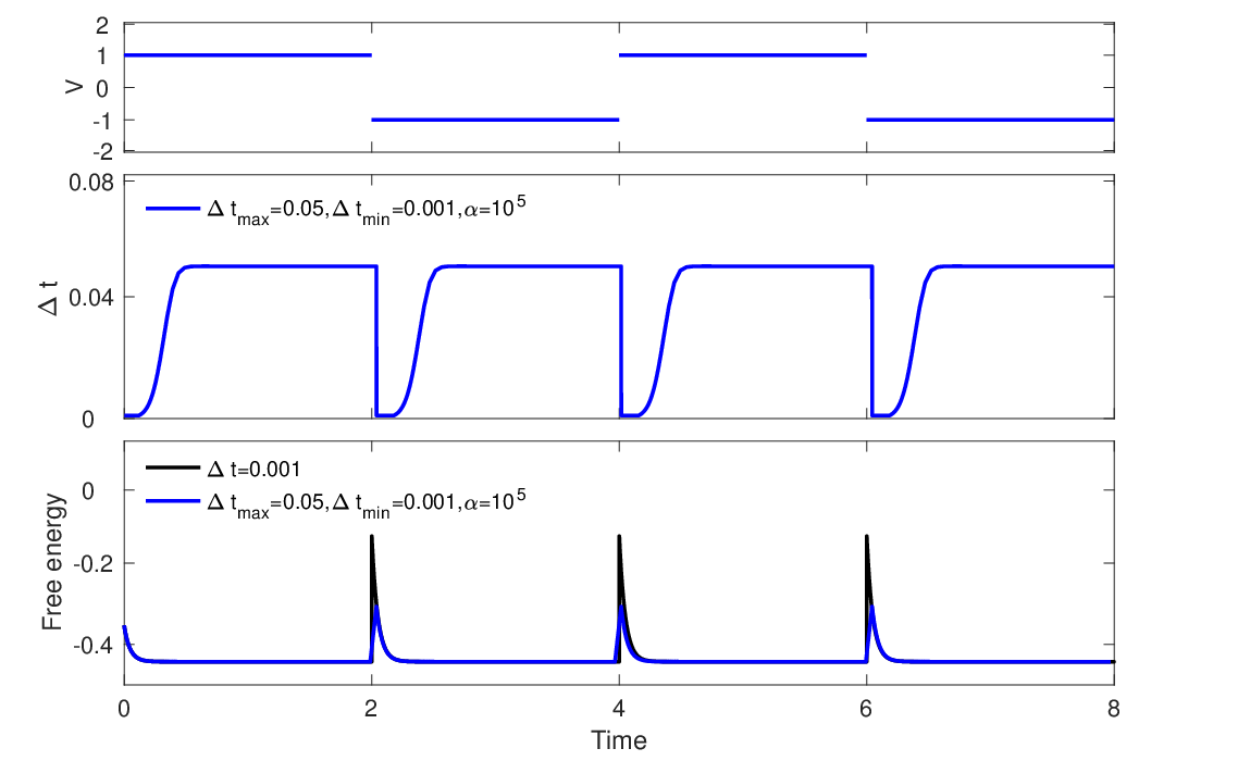
Figure 2: Upper: The evolution of the applied potential V⁡(t)V(t); Middle: The adaptive time stepping size versus time; Lower: Free-energy evolution with a uniform time-stepping size Δ​t=0.001\Delta t=0.001 (black) and adaptive time stepping sizes with parameters Δ​tmax=0.05\Delta t_{\text{max}}=0.05, Δ​tmin=0.001\Delta t_{\text{min}}=0.001, and α=105\alpha=10^{5} (blue).

We now study the time-marching stability of the numerical scheme and the efficiency improvement by using the strategy of adaptive time stepping in solving problems in which electrolytes are exposed to sudden alternating applied potentials. We consider the same initial and boundary conditions as in (43) except that ψ⁡(t,1,y)=V⁡(t)\psi(t,1,y)=V(t) for y∈[0,1]y\in[0,1] with

V⁡(t)=χ[0,2)−χ[2,4)+χ[4,6)−χ[6,8),V(t)=\chi_{[0,2)}-\chi_{[2,4)}+\chi_{[4,6)}-\chi_{[6,8)},

where χ[⋅,⋅)\chi_{[\cdot,\cdot)} is the characteristic function of a time interval. That is, a periodically alternating potential V⁡(t)V(t) is applied horizontally across the computational domain; cf. the upper plot of the Fig. 2.

We investigate the effectiveness of adaptive time-stepping techniques using the form of (19) with a parameter setting Δ​tmax=0.05\Delta t_{\text{max}}=0.05, Δ​tmin=0.001\Delta t_{\text{min}}=0.001, and α=105\alpha=10^{5}. The adaptive time step evolution is presented in the middle plot of the Fig. 2, and the corresponding free-energy evolution profile is displayed in the lower plot of the Fig. 2. For comparison, we also present the free-energy evolution profile computed with a uniform time step size (Δ​t=0.001\Delta t=0.001) in the same plot. As the applied potential changes periodically, the free energy correspondingly undergoes large, abrupt changes. This in turn leads to drastic decrease of the time stepping size to the minimum value Δ​tmin\Delta t_{\text{min}}. One can observe that, for a fixed applied potential, the free energy quickly relaxes and the corresponding time step size increases to its maximum value Δ​tmax\Delta t_{\text{max}}. In contrast to 80008000 steps with Δ​t=Δ​tmin=0.001\Delta t=\Delta t_{\text{min}}=0.001 to reach T=8T=8, the adaptive time stepping only takes a total of 877877 steps, which have about 89%89\% reduction in time steps. Of interest is that the free-energy evolution profile computed with adaptive time stepping is almost identical to that with Δ​t=0.001\Delta t=0.001, with minor discrepancy due to the resolution of time. This indicates that the strategy of adaptive time stepping is useful in speeding up computations of problems that have applied potentials with sudden changes.

5.4 Charge Dynamics

Refer to caption
Figure 3: The applied potential V⁡(t)V(t) with ω=15​π\omega=15\pi. It keeps as a constant for the time interval [0,1.5)[0,1.5) and continuously becomes a sinusoidal function for [1.5,+∞)[1.5,+\infty).

We apply the proposed numerical approaches to probe the charge dynamics in electrolytes between two parallel electrodes with sinusoidal applied potentials. Electrolytes under alternating current (AC) have wide range of applications, including AC electroosmosis (ACEO) pumps, cyclic voltammetry, and dielectrophoresis [4, 3, 1]. Numerical simulation with sinusoidal applied potentials of large frequency is computationally challenging. It sets high demand on the stability of numerical integration methods.

We consider a closed, neutral system that consists of binary monovalent ions. Due to geometry symmetry, the problem can be reduced to one dimension on a computational domain [−1,1][-1,1], after nondimensionalization. We consider the same initial and boundary conditions as in (43) except that the left electrode is kept grounded, i.e., ψ⁡(t,−1)=0\psi(t,-1)=0, and ψ⁡(t,1)=V⁡(t)\psi(t,1)=V(t) with

V(t)=χ[0,1.5)+χ[1.5,+∞)sin(ωt),V(t)=\chi_{[0,1.5)}+\chi_{[1.5,+\infty)}\sin\left(\omega t\right),

where ω\omega is the angular frequency; cf. Fig. 3.

Refer to caption
Figure 4: Evolution of cation distribution (upper row) and electrostatic potential (lower row) with various angular frequency ω\omega.

In Fig. 4, we consider the dynamics of concentrations and electrostatic potential with various angular frequency. For T<1.5T<1.5, the potential difference across two electrodes attracts oppositely charged ions from the bulk, forming electric double layers (EDLs) in the vicinity of electrodes. In the meantime, the electrostatic potential gets screened by the charges in the EDLs. After the charging phase, the boundary potential becomes sinusoidal and the electrostatic potential across the system responds instantaneously. The ionic concentration close to the electrodes oscillates correspondingly. However, the magnitude of oscillation decays as time evolves, because charges in the EDLs are gradually released to the bulk.

With larger angular frequency, the electrostatic potential inside still can follow the boundary potential instantaneously. However, the ionic concentration fall behind the potential oscillation and the potential only partially gets screened. At lower frequency, ions can travel much longer distances during each AC cycle; therefore, the oscillatory effect extend farther away from the electrode surface, with more pronounced impact on the structure of EDLs. For ω=39​π\omega=39\pi, we barely observe oscillations in concentration for 2<T<32<T<3.

Refer to caption
Figure 5: Evolution of total net charges ρ⁡(t)\rho(t) with various angular frequency ω\omega.

To further understand charge dynamics with sinusoidal applied potentials, we also study the evolution of total net charges in left half of the electrolytes [4]:

ρ⁡(t)=∫−10∑l=12ql​cl​(x)​𝑑x.\rho(t)=\int_{-1}^{0}\sum_{l=1}^{2}q^{l}c^{l}(x)dx.

As seen from Fig. 5, the total net charges increase quickly and reach a plateau with a constant applied voltage in the charging phase, i.e., 0<T<1.50<T<1.5. Later, the total net charges decay oscillatorily to zero at T=3T=3, which indicates that the discharging phase with sinusoidal applied potentials takes roughly the same time as the charging phase. For lower angular frequency, the total net charges have larger magnitude of oscillation, being consistent with the results shown in Fig. 4. For ω=95​π\omega=95\pi, the oscillation in the profile of ρ⁡(t)\rho(t) is extremely small. Larger angular frequency leads to shrinking oscillation magnitude, indicating that the effect of applied potentials with rather large frequency is equivalent to a zero applied potential. This observation is further confirmed by the lower plot in the Fig. 5, which is obtained with a zero applied potential (ω=0\omega=0) for T>1.5T>1.5. We can see that the profile of the total net charges is almost identical to the case with ω=95​π\omega=95\pi.

6 Conclusions

The Poisson–Nernst–Planck (PNP) equations are a classical model to describe ion transport, which is fundamental to many applications. In this work, we have developed finite difference schemes for solving the multi-dimensional PNP equations with multiple ionic species. Numerical analysis has shown that the schemes are able to guarantee mass conservation, positivity, and free-energy dissipation at fully discrete level. The novelty of numerical schemes lies in using the harmonic-mean approximations in the spatial discretization of the Nernst–Planck equations. In addition, we have proposed a new Newton’s method to efficiently solve a fully implicit nonlinear system resulting from discretization. The improved computational efficiency of the Newton’s method originates from the usage of the electrostatic potential as the iteration variable, instead of both the potential and concentration of multiple ionic species. Thanks to the harmonic-mean approximations, we have been able to rigorously establish the solvability and stability of the linearized problem in the Newton’s method and estimates on the upper bound of condition numbers of coefficient matrices in linear systems that are solved iteratively. Extensive numerical tests have been performed to corroborate the anticipated numerical accuracy, computational efficiency, and structure-preserving properties of the developed schemes. Also, numerical simulations have shown that a strategy of adaptive time stepping is able to speed up simulation of problems with time-dependent, alternating boundary potentials. Finally, the proposed numerical approaches have been applied to understand ion transport in response to a sinusoidal applied potential. Such numerical simulations demonstrate that the developed numerical approaches are promising in solving complex, realistic ion transport problems.

We now discuss several issues and possible further refinements of our work. The current development of numerical methods only considers a regular domain. However, it is of practical interest to extend the developed numerical methods for irregular computational domains, such as irregular geometry considered in ion-channel applications. The discretization accuracy on irregular boundaries deserves further attention, and discrete structure-preserving properties, such as positivity preservation and mass conservation, are highly desirable to maintain. Because these numerical properties are crucial to the validity of numerical solutions. It is also desirable to pursue second-order temporal discretization schemes that have structure-preserving properties. In addition, it will be our future work to extend the proposed discretization schemes and the Newton’s method to solve other modified PNP models that account for steric effects, Coulomb ionic correlations, and inhomogeneous dielectric effects [27, 3, 23, 37, 24, 33, 20].

Acknowledgments. J. Ding was supported by Postgraduate Research & Practice Innovation Program of Jiangsu Province and National Natural Science Foundation of China (No. 21773165, 11601361, 11771318, and 11790274). S. Zhou was supported by National Natural Science Foundation of China (No. 21773165 and 11601361) and National Key R&D Program of China (No. 2018YFB0204404).

Appendix A Appendix: the matrix 𝒦⁡(𝝁l,𝒖)\mathcal{K}(\boldsymbol{\mu}^{l},\boldsymbol{u})

To facilitate the presentation, we denote by Sl=ql​𝒖S^{l}=q^{l}\boldsymbol{u} and introduce the following discrete operators

ℰx±​Si,jl,n=eSi±1,jl,n−Si,jl,n(1+eSi±1,jl,n−Si,jl,n)2,ℰy±​Si,jl,n=eSi,j±1l,n−Si,jl,n(1+eSi,j±1l,n−Si,jl,n)2.\mathcal{E}^{\pm}_{x}S^{l,n}_{i,j}=\frac{e^{S^{l,n}_{i\pm 1,j}-S^{l,n}_{i,j}}}{(1+e^{S^{l,n}_{i\pm 1,j}-S^{l,n}_{i,j}})^{2}},~\mathcal{E}^{\pm}_{y}S^{l,n}_{i,j}=\frac{e^{S^{l,n}_{i,j\pm 1}-S^{l,n}_{i,j}}}{(1+e^{S^{l,n}_{i,j\pm 1}-S^{l,n}_{i,j}})^{2}}.

We now examine elements in each column of the matrix 𝒦\mathcal{K}. For the kkth column with k=[i,j]k=[i,j], the column elements are related to coefficients in the discretization stencils of the Nernst–Planck equations, associated to the grid point {xi,yj}\{x_{i},y_{j}\}. Thus, we look into all of the discretization stencils for different types of grid points.

First, for any interior grid point {xi,yj}\{x_{i},y_{j}\} with i=2,…,Nx−1i=2,\dots,N_{x}-1 and j=2,…,Ny−1j=2,\dots,N_{y}-1, non-zero entries of the kkth column (k=[i,j]k=[i,j]) are given by

𝒦m,kl={−2​Δ​tn+1​hjyhi−12x​ℰx−​Si,jl,n​μm+Nyl,n−2​Δ​tn+1​hjyhi−12x​ℰx+​Si−1,jl,n​μml,n,m=[i−1,j],−2​Δ​tn+1​hixhj−12y​ℰy+​Si,j−1l,n​μml,n−2​Δ​tn+1​hixhj−12y​ℰy−​Si,jl,n​μm+1l,n,m=[i,j−1],2​Δ​tn+1​(hjyhi+12x​ℰx+​Si,jl,n+hjyhi−12x​ℰx−​Si,jl,n+hixhj+12y​ℰy+​Si,jl,n+hixhj−12y​ℰy−​Si,jl,n)​μml,n+2​Δ​tn+1​hjyhi−12x​ℰx+​Si−1,jl,n​μm−Nyl,n+2​Δ​tn+1​hjyhi+12x​ℰx−​Si+1,jl,n​μm+Nyl,n+2​Δ​tn+1​hixhj+12y​ℰy−​Si,j+1l,n​μm+1l,n+2​Δ​tn+1​hixhj−12y​ℰy+​Si,j−1l,n​μm−1l,n,m=k,−2​Δ​tn+1​hixhj+12y​ℰy−​Si,j+1l,n​μm+1l,n−2​Δ​tn+1​hixhj+12y​ℰy+​Si,jl,n​μml,n,m=[i,j+1],−2​Δ​tn+1​hjyhi+12x​ℰx−​Si+1,jl,n​μm+Nyl,n−2​Δ​tn+1​hjyhi+12x​ℰx+​Si,jl,n​μml,n,m=[i+1,j].\mathcal{K}^{l}_{m,k}=\left\{\begin{aligned} &-2\Delta t^{n+1}\frac{h^{y}_{j}}{h^{x}_{i-\frac{1}{2}}}\mathcal{E}^{-}_{x}S^{l,n}_{i,j}\mu^{l,n}_{m+N_{y}}-2\Delta t^{n+1}\frac{h^{y}_{j}}{h^{x}_{i-\frac{1}{2}}}\mathcal{E}^{+}_{x}S^{l,n}_{i-1,j}\mu^{l,n}_{m},\quad m=[i-1,j],\\ &-2\Delta t^{n+1}\frac{h^{x}_{i}}{h^{y}_{j-\frac{1}{2}}}\mathcal{E}^{+}_{y}S^{l,n}_{i,j-1}\mu^{l,n}_{m}-2\Delta t^{n+1}\frac{h^{x}_{i}}{h^{y}_{j-\frac{1}{2}}}\mathcal{E}^{-}_{y}S^{l,n}_{i,j}\mu^{l,n}_{m+1},\quad m=[i,j-1],\\ &2\Delta t^{n+1}\left(\frac{h^{y}_{j}}{h^{x}_{i+\frac{1}{2}}}\mathcal{E}^{+}_{x}S^{l,n}_{i,j}+\frac{h^{y}_{j}}{h^{x}_{i-\frac{1}{2}}}\mathcal{E}^{-}_{x}S^{l,n}_{i,j}+\frac{h^{x}_{i}}{h^{y}_{j+\frac{1}{2}}}\mathcal{E}^{+}_{y}S^{l,n}_{i,j}+\frac{h^{x}_{i}}{h^{y}_{j-\frac{1}{2}}}\mathcal{E}^{-}_{y}S^{l,n}_{i,j}\right)\mu^{l,n}_{m}\\ &\quad+2\Delta t^{n+1}\frac{h^{y}_{j}}{h^{x}_{i-\frac{1}{2}}}\mathcal{E}^{+}_{x}S^{l,n}_{i-1,j}\mu^{l,n}_{m-N_{y}}+2\Delta t^{n+1}\frac{h^{y}_{j}}{h^{x}_{i+\frac{1}{2}}}\mathcal{E}^{-}_{x}S^{l,n}_{i+1,j}\mu^{l,n}_{m+N_{y}}\\ &\quad+2\Delta t^{n+1}\frac{h^{x}_{i}}{h^{y}_{j+\frac{1}{2}}}\mathcal{E}^{-}_{y}S^{l,n}_{i,j+1}\mu^{l,n}_{m+1}+2\Delta t^{n+1}\frac{h^{x}_{i}}{h^{y}_{j-\frac{1}{2}}}\mathcal{E}^{+}_{y}S^{l,n}_{i,j-1}\mu^{l,n}_{m-1},~m=k,\\ &-2\Delta t^{n+1}\frac{h^{x}_{i}}{h^{y}_{j+\frac{1}{2}}}\mathcal{E}^{-}_{y}S^{l,n}_{i,j+1}\mu^{l,n}_{m+1}-2\Delta t^{n+1}\frac{h^{x}_{i}}{h^{y}_{j+\frac{1}{2}}}\mathcal{E}^{+}_{y}S^{l,n}_{i,j}\mu^{l,n}_{m},\quad m=[i,j+1],\\ &-2\Delta t^{n+1}\frac{h^{y}_{j}}{h^{x}_{i+\frac{1}{2}}}\mathcal{E}^{-}_{x}S^{l,n}_{i+1,j}\mu^{l,n}_{m+N_{y}}-2\Delta t^{n+1}\frac{h^{y}_{j}}{h^{x}_{i+\frac{1}{2}}}\mathcal{E}^{+}_{x}S^{l,n}_{i,j}\mu^{l,n}_{m},\quad m=[i+1,j].\\ \end{aligned}\right.

Hence, the conclusion (38) holds for the columns associated to interior grid points. We examine the conclusion for boundary grid points that are adjacent to four edges but not corner vertices. We consider Dirichlet boundary grid points {x1,yj}\{x_{1},y_{j}\} for j=2,…,Ny−1j=2,\dots,N_{y}-1, and Neumann boundary grid points {xi,y1}\{x_{i},y_{1}\} for i=2,…,Nx−1i=2,\dots,N_{x}-1. Non-zero entries of the kkth column (k=[1,j]k=[1,j]) are

𝒦m,kl={−2​Δ​tn+1​h1xhj−12y​ℰy+​S1,j−1l,n​μml,n−2​Δ​tn+1​h1xhj−12y​ℰy−​S1,jl,n​μm+1l,n,m=[1,j−1],2​Δ​tn+1​(hjyh32x​ℰx+​S1,jl,n+h1xhj+12y​ℰy+​S1,jl,n+h1xhj−12y​ℰy−​S1,jl,n)​μml,n+2​Δ​tn+1​hjyh32x​ℰx−​S2,jl,n​μm+Nyl,n+2​Δ​tn+1​h1xhj+12y​ℰy−​S1,j+1l,n​μm+1l,n+2​Δ​tn+1​h1xhj−12y​ℰy+​S1,j−1l,n​μm−1l,n,m=k,−2​Δ​tn+1​h1xhj+12y​ℰy−​S1,j+1l,n​μml,n−2​Δ​tn+1​h1xhj+12y​ℰy+​S1,jl,n​μm−1l,n,m=[1,j+1],−2​Δ​tn+1​hjyh32x​ℰx−​S2,jl,n​μml,n−2​Δ​tn+1​hjyh32x​ℰx+​S1,jl,n​μm−Nyl,n,m=[2,j].\mathcal{K}^{l}_{m,k}=\left\{\begin{aligned} &-2\Delta t^{n+1}\frac{h^{x}_{1}}{h^{y}_{j-\frac{1}{2}}}\mathcal{E}^{+}_{y}S^{l,n}_{1,j-1}\mu^{l,n}_{m}-2\Delta t^{n+1}\frac{h^{x}_{1}}{h^{y}_{j-\frac{1}{2}}}\mathcal{E}^{-}_{y}S^{l,n}_{1,j}\mu^{l,n}_{m+1},\quad m=[1,j-1],\\ &2\Delta t^{n+1}\left(\frac{h^{y}_{j}}{h^{x}_{\frac{3}{2}}}\mathcal{E}^{+}_{x}S^{l,n}_{1,j}+\frac{h^{x}_{1}}{h^{y}_{j+\frac{1}{2}}}\mathcal{E}^{+}_{y}S^{l,n}_{1,j}+\frac{h^{x}_{1}}{h^{y}_{j-\frac{1}{2}}}\mathcal{E}^{-}_{y}S^{l,n}_{1,j}\right)\mu^{l,n}_{m}+2\Delta t^{n+1}\frac{h^{y}_{j}}{h^{x}_{\frac{3}{2}}}\mathcal{E}^{-}_{x}S^{l,n}_{2,j}\mu^{l,n}_{m+N_{y}}\\ &\quad+2\Delta t^{n+1}\frac{h^{x}_{1}}{h^{y}_{j+\frac{1}{2}}}\mathcal{E}^{-}_{y}S^{l,n}_{1,j+1}\mu^{l,n}_{m+1}+2\Delta t^{n+1}\frac{h^{x}_{1}}{h^{y}_{j-\frac{1}{2}}}\mathcal{E}^{+}_{y}S^{l,n}_{1,j-1}\mu^{l,n}_{m-1},~m=k,\\ &-2\Delta t^{n+1}\frac{h^{x}_{1}}{h^{y}_{j+\frac{1}{2}}}\mathcal{E}^{-}_{y}S^{l,n}_{1,j+1}\mu^{l,n}_{m}-2\Delta t^{n+1}\frac{h^{x}_{1}}{h^{y}_{j+\frac{1}{2}}}\mathcal{E}^{+}_{y}S^{l,n}_{1,j}\mu^{l,n}_{m-1},\quad m=[1,j+1],\\ &-2\Delta t^{n+1}\frac{h^{y}_{j}}{h^{x}_{\frac{3}{2}}}\mathcal{E}^{-}_{x}S^{l,n}_{2,j}\mu^{l,n}_{m}-2\Delta t^{n+1}\frac{h^{y}_{j}}{h^{x}_{\frac{3}{2}}}\mathcal{E}^{+}_{x}S^{l,n}_{1,j}\mu^{l,n}_{m-N_{y}},\quad m=[2,j].\\ \end{aligned}\right.

Non-zero entries of the kkth column (k=[i,1]k=[i,1]) are

𝒦m,kl={−2​Δ​tn+1​h1yhi−12x​ℰx−​Si,1l,n​μm+Nyl,n−2​Δ​tn+1​h1yhi−12x​ℰx+​Si−1,1l,n​μml,n,m=[i−1,1],2​Δ​tn+1​(h1yhi+12x​ℰx+​Si,1l,n+h1yhi−12x​ℰx−​Si,1l,n+hixh32y​ℰy+​Si,1l,n)​μml,n+2​Δ​tn+1​h1yhi−12x​ℰx+​Si−1,1l,n​μm−Nyl,n+2​Δ​tn+1​h1yhi+12x​ℰx−​Si+1,1l,n​μm+Nyl,n+2​Δ​tn+1​hixh32y​ℰy−​Si,2l,n​μm+1l,n,m=k,−2​Δ​tn+1​hixh32y​ℰy−​Si,2l,n​μml,n−2​Δ​tn+1​hixh32y​ℰy+​Si,1l,n​μm−1l,n,m=[i,2],−2​Δ​tn+1​h1yhi+12x​ℰx−​Si+1,1l,n​μml,n−2​Δ​tn+1​h1yhi+12x​ℰx+​Si,1l,n​μm−Nyl,n,m=[i+1,1].\mathcal{K}^{l}_{m,k}=\left\{\begin{aligned} &-2\Delta t^{n+1}\frac{h^{y}_{1}}{h^{x}_{i-\frac{1}{2}}}\mathcal{E}^{-}_{x}S^{l,n}_{i,1}\mu^{l,n}_{m+N_{y}}-2\Delta t^{n+1}\frac{h^{y}_{1}}{h^{x}_{i-\frac{1}{2}}}\mathcal{E}^{+}_{x}S^{l,n}_{i-1,1}\mu^{l,n}_{m},\quad m=[i-1,1],\\ &2\Delta t^{n+1}\left(\frac{h^{y}_{1}}{h^{x}_{i+\frac{1}{2}}}\mathcal{E}^{+}_{x}S^{l,n}_{i,1}+\frac{h^{y}_{1}}{h^{x}_{i-\frac{1}{2}}}\mathcal{E}^{-}_{x}S^{l,n}_{i,1}+\frac{h^{x}_{i}}{h^{y}_{\frac{3}{2}}}\mathcal{E}^{+}_{y}S^{l,n}_{i,1}\right)\mu^{l,n}_{m}+2\Delta t^{n+1}\frac{h^{y}_{1}}{h^{x}_{i-\frac{1}{2}}}\mathcal{E}^{+}_{x}S^{l,n}_{i-1,1}\mu^{l,n}_{m-N_{y}}\\ &\quad+2\Delta t^{n+1}\frac{h^{y}_{1}}{h^{x}_{i+\frac{1}{2}}}\mathcal{E}^{-}_{x}S^{l,n}_{i+1,1}\mu^{l,n}_{m+N_{y}}+2\Delta t^{n+1}\frac{h^{x}_{i}}{h^{y}_{\frac{3}{2}}}\mathcal{E}^{-}_{y}S^{l,n}_{i,2}\mu^{l,n}_{m+1},~m=k,\\ &-2\Delta t^{n+1}\frac{h^{x}_{i}}{h^{y}_{\frac{3}{2}}}\mathcal{E}^{-}_{y}S^{l,n}_{i,2}\mu^{l,n}_{m}-2\Delta t^{n+1}\frac{h^{x}_{i}}{h^{y}_{\frac{3}{2}}}\mathcal{E}^{+}_{y}S^{l,n}_{i,1}\mu^{l,n}_{m-1},\quad m=[i,2],\\ &-2\Delta t^{n+1}\frac{h^{y}_{1}}{h^{x}_{i+\frac{1}{2}}}\mathcal{E}^{-}_{x}S^{l,n}_{i+1,1}\mu^{l,n}_{m}-2\Delta t^{n+1}\frac{h^{y}_{1}}{h^{x}_{i+\frac{1}{2}}}\mathcal{E}^{+}_{x}S^{l,n}_{i,1}\mu^{l,n}_{m-N_{y}},\quad m=[i+1,1].\\ \end{aligned}\right.

Thus, we can verify that the conclusion (38) holds for the columns associated to edge grid points. For corner vertices grid points, e.g., k=[1,1]k=[1,1], we have

𝒦m,kl={2​Δ​tn+1​(h1yh32x​ℰx+​S1,1l,n+h1xh32y​ℰy+​S1,1l,n)​μml,n+2​Δ​tn+1​h1yh32x​ℰx−​S2,1l,n​μm+Nyl,n+2​Δ​tn+1​h1xh32y​ℰy−​S1,2l,n​μm+1l,n,m=k,−2​Δ​tn+1​h1xh32y​ℰy−​S1,2l,n​μml,n−2​Δ​tn+1​h1xh32y​ℰy+​S1,1l,n​μm−1l,n,m=[1,2],−2​Δ​tn+1​h1yh32x​ℰx−​S2,1l,n​μml,n−2​Δ​tn+1​h1yh32x​ℰx+​S1,1l,n​μm−Nyl,n,m=[2,1].\mathcal{K}^{l}_{m,k}=\left\{\begin{aligned} &2\Delta t^{n+1}\left(\frac{h^{y}_{1}}{h^{x}_{\frac{3}{2}}}\mathcal{E}^{+}_{x}S^{l,n}_{1,1}+\frac{h^{x}_{1}}{h^{y}_{\frac{3}{2}}}\mathcal{E}^{+}_{y}S^{l,n}_{1,1}\right)\mu^{l,n}_{m}+2\Delta t^{n+1}\frac{h^{y}_{1}}{h^{x}_{\frac{3}{2}}}\mathcal{E}^{-}_{x}S^{l,n}_{2,1}\mu^{l,n}_{m+N_{y}}\\ &\quad+2\Delta t^{n+1}\frac{h^{x}_{1}}{h^{y}_{\frac{3}{2}}}\mathcal{E}^{-}_{y}S^{l,n}_{1,2}\mu^{l,n}_{m+1},~m=k,\\ &-2\Delta t^{n+1}\frac{h^{x}_{1}}{h^{y}_{\frac{3}{2}}}\mathcal{E}^{-}_{y}S^{l,n}_{1,2}\mu^{l,n}_{m}-2\Delta t^{n+1}\frac{h^{x}_{1}}{h^{y}_{\frac{3}{2}}}\mathcal{E}^{+}_{y}S^{l,n}_{1,1}\mu^{l,n}_{m-1},\quad m=[1,2],\\ &-2\Delta t^{n+1}\frac{h^{y}_{1}}{h^{x}_{\frac{3}{2}}}\mathcal{E}^{-}_{x}S^{l,n}_{2,1}\mu^{l,n}_{m}-2\Delta t^{n+1}\frac{h^{y}_{1}}{h^{x}_{\frac{3}{2}}}\mathcal{E}^{+}_{x}S^{l,n}_{1,1}\mu^{l,n}_{m-N_{y}},\quad m=[2,1].\\ \end{aligned}\right.

Other corner vertices can be verified analogously. Also, we can verify that 𝒦\mathcal{K} is a symmetric matrix.

Without any assumption on Si,jl,nS^{l,n}_{i,j}, we have

0<ℰk±​Si,jl,n≤14​for​k=x,y.0<\mathcal{E}^{\pm}_{k}S^{l,n}_{i,j}\leq\frac{1}{4}~~\mbox{for}~k=x,y. (A.1)

Therefore, we have the following results:

{∑m=1Nx​Ny𝒦m,nl=∑n=1Nx​Ny𝒦m,nl=0for​m,n=1,…,Nx​Ny,0<𝒦n,nl<2​Δ​tn+1​(hMyhmx+hMxhmy)​‖𝝁l‖∞for​n=1,…,Nx​Ny,−Δ​tn+1​max⁡{hMyhmx,hMxhmy}​‖𝝁l‖∞<𝒦m,nl<0for​n,m=1,…,Nx​Ny,and​m≠n.\left\{\begin{aligned} &\sum_{m=1}^{N_{x}N_{y}}\mathcal{K}^{l}_{m,n}=\sum_{n=1}^{N_{x}N_{y}}\mathcal{K}^{l}_{m,n}=0\quad\mbox{for}~m,n=1,\dots,N_{x}N_{y},\\ &0<\mathcal{K}^{l}_{n,n}<2\Delta t^{n+1}(\frac{h^{y}_{M}}{h^{x}_{m}}+\frac{h^{x}_{M}}{h^{y}_{m}})\|\boldsymbol{\mu}^{l}\|_{\infty}\quad\mbox{for}~n=1,\dots,N_{x}N_{y},\\ &-\Delta t^{n+1}\max\{\frac{h^{y}_{M}}{h^{x}_{m}},\frac{h^{x}_{M}}{h^{y}_{m}}\}\|\boldsymbol{\mu}^{l}\|_{\infty}<\mathcal{K}^{l}_{m,n}<0\quad\mbox{for}~n,m=1,\dots,N_{x}N_{y},~\mbox{and}~m\neq n.\end{aligned}\right.

References

  • [1] S. M. H. H. Amrei, S. C. Bukosky, S. P. Rader, W. D. Ristenpart, and G. H. Miller. Oscillating electric fields in liquids create a long-range steady field. Phys. Rev. Lett., 121:185504, 2018.
  • [2] A. Arnold, P. Markowich, and G. Toscani. On large time asymptotics for drift-diffusion-Poisson systems. Transp. Theory Stat. Phys., 29(3-5):571–58, 2000.
  • [3] M. Bazant, M. S. Kilic, B. D. Storey, and A. Ajdari. Towards an understanding of induced-charge electrokinetics at large applied voltages in concentrated solutions. Adv. Colloid. Interface Sci., 152:48–88, 2009.
  • [4] M. Bazant, K. Thornton, and A. Ajdari. Diffuse-charge dynamics in electrochemical systems. Phys. Rev. E, 70(2):021506, 2004.
  • [5] P. Biler and J. Dolbeault. Long time behavior of solutions to Nernst-Planck and Debye-Hückel drift-diffusion systems. Ann. Henri Poincaré, 1(3):461–472, 2000.
  • [6] P. Biler, W. Hebisch, and T. Nadzieja. The Debye system: existence and large time behavior of solutions. Nonlinear Anal., 23:1189–1209, 1994.
  • [7] A. Cardenas, R. Coalson, and M. Kurnikova. Three-dimensional Poisson-Nernst-Planck theory studies: influence of membrane electrostatics on gramicidin A channel conductance. Biophys. J., 79(1):80–93, 2000.
  • [8] J. Chaudhry, J. Comer, A. Aksimentiev, and L. Olson. A stabilized finite element method for modified Poisson-Nernst-Planck equations to determine ion flow through a nanopore. Commun. Comput. Phys., 15:93–125, 2014.
  • [9] J. Ding, H. Sun, Z. Wang, and S. Zhou. Computational study on hysteresis of ion channels: Multiple solutions to steady-state Poisson–Nernst–Planck equations. Commun. Comput. Phys., 23(5):1549–1572, 2018.
  • [10] J. Ding, C. Wang, and S. Zhou. Optimal rate convergence analysis of a second order numerical scheme for the Poisson–Nernst–Planck system. Numer. Math. Theor. Meth. Appl., 12:607–626, 2019.
  • [11] J. Ding, Z. Wang, and S. Zhou. Positivity preserving finite difference methods for poisson–nernst–planck equations with steric interactions: Application to slit-shaped nanopore conductance. J. Comput. Phys., 397:108864, 2019.
  • [12] W. Fang and K. Ito. Asymptotic behavior of the drift-diffusion semiconductor equations. J. Differ. Equ., 123:567–587, 1995.
  • [13] W. Fang and K. Ito. Global solutions of the time-dependent drift-diffusion semiconductor equations. J. Differ. Equ., 123:523–566, 1995.
  • [14] A. Flavell, J. Kabre, and X. Li. An energy-preserving discretization for the Poisson-Nernst-Planck equations. J. Comput. Electron., 16:431–441, 2017.
  • [15] A. Flavell, M. Machen, R. Eisenberg, J. Kabre, C. Liu, and X. Li. A conservative finite difference scheme for Poisson-Nernst-Planck equations. J. Comput. Electron., 13:235–249, 2014.
  • [16] H. Gajewski and K. Gärtner. On the discretization of Van Roosbroeck’s equations with magnetic field. Z. Angew. Math. Mech., 76(5):247–264, 1996.
  • [17] H. Gajewski and K. Gröger. On the basic equations for carrier transport in semiconductors. J. Math. Anal. Appl., 113:12–35, 1986.
  • [18] H. Gao and D. He. Linearized conservative finite element methods for the Nernst–Planck–Poisson equations. J. Sci. Comput., 72:1269–1289, 2017.
  • [19] H. Gao and P. Sun. A linearized conservative mixed finite element method for Poisson–Nernst–Planck equations. J. Sci. Comput., 77:793–817, 2018.
  • [20] N. Gavish, C. Liu, and B. Eisenberg. Do bistable steric Poisson–Nernst–Planck models describe single-channel gating? J. Phys. Chem. B, 22(20):5183–5192, 2018.
  • [21] G. Golub and C. Loan. Matrix Computations. Johns Hopkins Studies in the Mathematical Sciences. Johns Hopkins University Press, 1996.
  • [22] J. Hu and X. Huang. A fully discrete positivity-preserving and energy-dissipative finite difference scheme for Poisson–Nernst–Planck equations. Submitted, 2019.
  • [23] Y. Hyon, B. Eisenberg, and C. Liu. A mathematical model for the hard sphere repulsion in ionic solutions. Commun. Math. Sci., 9:459–475, 2010.
  • [24] Y. Hyon, C. Liu, and B. Eisenberg. PNP equations with steric effects: a model of ion flow through channels. J. Phys. Chem. B, 116:11422–11441, 2012.
  • [25] J. Jiang, D. Cao, D. Jiang, and J. Wu. Time-dependent density funcational theory for ion diffusion in electrochemical systems. J. Phys.: Condens. Matter., 26:284102, 2014.
  • [26] M. Kilic, M. Bazant, and A. Ajdari. Steric effects in the dynamics of electrolytes at large applied voltages. II. Modified Poisson–Nernst–Planck equations. Phys. Rev. E, 75:021503, 2007.
  • [27] M. S. Kilic, M. Bazant, and A. Ajdari. Steric effects in the dynamics of electrolytes at large applied voltages. I. Double-layer charging. Phys. Rev. E, 75:021502, 2007.
  • [28] B. Li, P. Liu, Z. Xu, and S. Zhou. Ionic size effects: generalized boltzmann distributions, counterion stratification, and modified debye length. Nonlinearity, 26(10):2899, 2013.
  • [29] X. Li, Z. Qiao, and H. Zhang. An unconditionally energy stable finite difference scheme for a stochastic Cahn-Hilliard equation. Science China Mathematics, 59(9):1815–1834, 2016.
  • [30] T. Lin and B. Eisenberg. A new approach to the Lennard-Jones potential and a new model: PNP-steric equations. Commun. Math. Sci., 12:149–173, 2014.
  • [31] H. Liu and Z. Wang. A free energy satisfying finite difference method for Poisson-Nernst-Planck equations. J. Comput. Phys., 268:363–376, 2014.
  • [32] H. Liu and Z. Wang. A free energy satisfying discontinuous Galerkin method for one-dimensional Poisson-Nernst-Planck systems. J. Comput. Phys., 328:413–437, 2017.
  • [33] P. Liu, X. Ji, and Z. Xu. Modified Poisson–Nernst–Planck model with accurate Coulomb correlation in variable media. SIAM J. Appl. Math., 78:226–245, 2018.
  • [34] X. Liu, Y. Qiao, and B. Lu. Analysis of the mean field free energy functional of electrolyte solution with non-homogenous boundary conditions and the generalized PB/PNP equations with inhomogeneous dielectric permittivity. SIAM J. Appl. Math., 78:1131–1154, 2018.
  • [35] Y. Liu and C.-W. Shu. Analysis of the local discontinuous Galerkin method for the drift-diffusion model of semiconductor devices. Sci. China Math., 59:115–140, 2016.
  • [36] B. Lu, M. Holst, J. McCammon, and Y. Zhou. Poisson-Nernst-Planck equations for simulating biomolecular diffusion-reaction processes I: Finite element solutions. J. Comput. Phys., 229(19):6979–6994, 2010.
  • [37] B. Lu and Y. Zhou. Poisson-Nernst-Planck equations for simulating biomolecular diffusion-reaction processes II: Size effects on ionic distributions and diffusion-reaction rates. Biophys. J., 100:2475–2485, 2011.
  • [38] P. Markowich. The Stationary Semiconductor Device Equations. Springer-Verlag, New York, 1986.
  • [39] D. Meng, B. Zheng, G. Lin, and M. Sushko. Numerical solution of 3D Poisson-Nernst-Planck equations coupled with classical density functional theory for modeling ion and electron transport in confined environment. Commun. Comput. Phys., 16:1298–1322, 2014.
  • [40] M. Metti, J. Xu, and C. Liu. Energetically stable discretizations for charge transport and electrokinetic models. J. Comput. Phys., 306:1–18, 2016.
  • [41] M. Mirzadeh and F. Gibou. A conservative discretization of the Poisson-Nernst-Planck equations on adaptive cartesian grids. J. Comput. Phys., 274:633–653, 2014.
  • [42] M. Mock. An initial value problem from semiconductor device theory. SIAM J. Math. Anal., 5:597–612, 1974.
  • [43] A. Prohl and M. Schmuck. Convergent discretizations for the Nernst–Planck–Poisson system. Numer. Math., 111:591–630, 2009.
  • [44] Y. Qian, Z. Wang, and S. Zhou. A conservative, free energy dissipating, and positivity preserving finite difference scheme for multi-dimensional nonlocal Fokker–Planck equation. J. Comput. Phys., 386:22–36, 2019.
  • [45] Y. Qiao, X. Liu, M. Chen, and B. Lu. A local approximation of fundamental measure theory incorporated into three dimensional Poisson–Nernst–Planck equations to account for hard sphere repulsion among ions. J. Stat. Phys., 163:156–174, 2016.
  • [46] Y. Qiao, B. Tu, and B. Lu. Ionic size effects to molecular solvation energy and to ion current across a channel resulted from the nonuniform size-modified PNP equations. J. Chem. Phys., 140:174102, 2014.
  • [47] Z. Qiao, Z. Zhang, and T. Tang. An adaptive time-stepping strategy for the molecular beam epitaxy models. SIAM J. Sci. Comput., 33:1395–1414, 2011.
  • [48] R. Schoch, J. Han, and P. Renaud. Transport phenomena in nanofluidics. Rev. Mod. Phys., 80:839–883, 2008.
  • [49] F. Siddiqua, Z. Wang, and S. Zhou. A modified Poisson–Nernst–Planck model with excluded volume effect: theory and numerical implementation. Commun. Math. Sci., 16 (1):251–271, 2018.
  • [50] Y. Sun, P. Sun, B. Zheng, and G. Lin. Error analysis of finite element method for Poisson–Nernst–Planck equations. J. Comput. Appl. Math., 301:28–43, 2016.
  • [51] N. Wang, S. Zhou, P. Kekenes-Huskey, B. Li, and J. A. McCammon. Poisson-Boltzmann vs. Size-modified Poisson-Boltzmann electrostatics applied to lipid bilayers. J. Phys. Chem. B, 118(51):14827–14832, 2014.
  • [52] Z. Xu, M. Ma, and P. Liu. Self-energy-modified Poisson–Nernst–Planck equations: WKB approximation and finite-difference approaches. Phys. Rev. E, 90:013307, 2014.
  • [53] J. Zheng and M. Trudeau. Handbook of ion channels. CRC Press, 2015.
  • [54] Q. Zheng, D. Chen, and G. Wei. Second-order Poisson-Nernst-Planck solver for ion channel transport. J. Comput. Phys., 230(13):5239–5262, 2011.
  • [55] S. Zhou, Z. Wang, and B. Li. Mean-field description of ionic size effects with non-uniform ionic sizes: A numerical approach. Phys. Rev. E, 84:021901, 2011.