Stochastic Normalizing Flows
Abstract
We introduce stochastic normalizing flows, an extension of continuous normalizing flows for maximum likelihood estimation and variational inference (VI) using stochastic differential equations (SDEs). Using the theory of rough paths, the underlying Brownian motion is treated as a latent variable and approximated, enabling efficient training of neural SDEs as random neural ordinary differential equations. These SDEs can be used for constructing efficient Markov chains to sample from the underlying distribution of a given dataset. Furthermore, by considering families of targeted SDEs with prescribed stationary distribution, we can apply VI to the optimization of hyperparameters in stochastic MCMC.
1 Introduction
Normalizing flows (Rezende & Mohamed 2015) are probabilistic models constructed as a sequence of successive transformations applied to some initial distribution. A key strength of normalizing flows is their expressive power as generative models, while enjoying an explicitly computable form of the likelihood function evaluated on the transformed space. This makes them especially well-equipped for variational inference (VI). Neural networks are often used as inspiration for finding effective transformations (Dinh et al. 2015; van den Berg et al. 2018).
Continuous normalizing flows were later developed in Chen et al. 2018 as a means to perform maximum likelihood estimation and VI for large-scale probabilistic models derived from ordinary differential equations (ODEs). The framework stems from the computation of the evolving density of an ODE with random initial value, as the solution to another ODE. The jump to continuous-time dynamics affords a few computational benefits over its discrete-time counterpart, namely the presence of a trace in place of a determinant in the evolution formulae for the density, as well as the adjoint method for memory-efficient backpropagation. Motivated by deep learning, a family of ODEs, called neural ordinary differential equations were constructed, whose Euler discretizations resembled layer-wise transformations of residual neural networks. Further algorithmic improvements to the framework were presented by Grathwohl et al. 2018, enabling virtually arbitrary choices of parameterized classes of ODEs. Doing all this involves some technical subtlety, and effective neural ODE architectures remain the subject of ongoing research — see for example (Dupont et al. 2019; Gholami et al. 2019; Zhang et al. 2019).
There has also been recent interest in extending these frameworks to a stochastic scenario, that is, training probabilistic models derived from stochastic differential equations (SDEs). For physical models, where the evolution of a dynamical system is no longer deterministic, or microscopic fluctuations are dependent on components changing too rapidly to quantify, an SDE can be more appropriate. Stochastic extensions of neural ODEs have been considered in (Tzen & Raginsky 2019; Liu et al. 2019; Jia & Benson 2019; Peluchetti & Favaro 2019) as limits of deep latent Gaussian models, where they have been suggested to show increased robustness to noisy / adversarial data. Furthermore, unlike deterministic flows, there is a foolproof recipe for constructing a family of SDEs that are ergodic with respect to some target distribution (Ma et al. 2015). This particular property guarantees the convergence of the solution of an SDE to a prescribed target distribution. Such SDEs are prime candidates for the construction of stochastic MCMC algorithms, by generating sample paths via approximate stochastic integration methods.
However, developing an analogue of the continuous normalizing flows framework for flows constructed from SDEs—in particular, one that comes with simple and rigorous mathematical theory and that does not rely on ad hoc or problem-specific assumptions—is far from trivial. A common approach for conducting VI with SDEs is to rely on Girsanov’s theorem. This allows one to estimate the Kullback-Leibler divergence between densities of solutions to two SDEs (for the prior and posterior distributions) with differing drift coefficients (Beskos et al. 2006; Tzen & Raginsky 2019). Following this approach, Li et al. 2020 developed a stochastic adjoint method which scales well to high dimensions, and enables SDEs as latent models in variational autoencoders. Theoretical justification of the method proved challenging, as stochastic calculus is ill-suited for analyzing backward (approximate) solutions to SDEs. Notable deficiencies with these previous approaches include difficulties with non-diagonal diffusion, incompatibility with higher-order adaptive SDE solvers, and a complex means of reconstructing Brownian motion paths from random number generator seeds. Furthermore, the method cannot be justifiably combined with existing approaches of density estimation for SDEs (see Hurn et al. 2007).
On the other hand, recent efforts have made significant strides in applying variational and MCMC methods for idealized Bayesian computation. One of the most significant contributions in this direction is Salimans et al. 2015, who performed VI with respect to distributions formed from steps of a reversible Markov chain. For example, the setting of Hamiltonian Monte Carlo was examined in Wolf et al. 2016. More recently, Liu & Feng 2016 considered optimizing step size in stochastic gradient Langevin dynamics using methods derived from kernelized Stein discrepancy. Langevin flows (Rezende & Mohamed 2015) have been discussed as a potential VI framework that takes inspiration from the SDEs underlying stochastic MCMC (Ma et al. 2015). Once again, implementation of Langevin flows relies on the approximation of the log-likelihood for a general class of SDEs.
Contributions
We provide a general theoretical framework (which we refer to as stochastic normalizing flows) for approximating generative models constructed from SDEs using continuous normalizing flows. These approximations can then be trained using existing techniques. By this process, we find that theoretical and practical developments concerning continuous normalizing flows and neural ODEs extend readily to the stochastic setting, without the need of an independent framework. The key theoretical enabler underlying our strong results and simple analysis is the theory of rough paths (Friz & Hairer 2014), an alternative stochastic calculus that enables approximation and pathwise treatment of SDEs. Our approach
- 1.
enables (i) density estimation, (ii) maximum likelihood estimation, and (iii) variational approximations beyond autoencoders, for arbitrary SDE models; and
- 2.
is easily implemented using any general continuous normalizing flows implementation, such as that of Grathwohl et al. 2018.
Our framework recovers the stochastic adjoint method of Li et al. 2020, but our approach is sufficiently flexible to overcome its deficiencies. Moreover, using our approach, any existing neural ODE framework (such as Zhang et al. 2019) can be extended to SDEs, simply by the addition of a few extra terms.
Following a review of background material in §2, the stochastic normalizing flows framework is introduced and discussed in §3, with our main approximation result presented in Theorem 2. Some numerical investigations are conducted in §4, including an application to hyperparameter optimization in stochastic MCMC.
2 Background Review
2.1 Continuous Normalizing Flows
We shall begin by reviewing the continuous normalizing flow framework for training ODE models, as our development of random and stochastic normalizing flows will build upon it. Consider a parameterized class of models of the following form: for , let satisfy the ODE with random initial condition (often called a random ordinary differential equation)
| (1) |
In a general machine learning context, one might choose such that the Euler discretization of (1) resembles layer-wise updates of a residual neural network (Lu et al. 2017; Chen et al. 2018), or one may parameterize as a neural network itself (Grathwohl et al. 2018). The resulting ODEs constitute the class of so-called neural ordinary differential equations. The following theorem is a consequence of the Liouville equation (equivalently, Fokker-Planck equation) applied to the solution of the random ODE (1), and it yields an ODE for the log density of evaluated at .
Theorem 1 (Chen et al. 2018).
Suppose that satisfies (1). The distribution of is absolutely continuous with respect to Lebesgue measure, with probability density satisfying
| (2) |
Naively computing the divergence in (2) with automatic differentiation is of quadratic complexity in the dimension . As pointed out by Grathwohl et al. 2018, this can be improved to linear complexity using a trace estimator (Roosta & Ascher 2015):
| (3) |
where each is an independent and identically distributed copy of a random vector with zero mean and . Common choices for include standard normal and Rademacher random vectors.
2.2 The Adjoint Method
Training continuous normalizing flows often involves minimizing a scalar loss function involving and/or the log-density computed via Theorem 1 with respect to the parameters . For this, we require gradients of with respect to for . The most obvious approach is to directly backpropagate through a numerical integration scheme such as in Ryder et al. 2018, but this does not scale well in . The superior alternative is the adjoint method, which computes derivatives of a scalar loss function by solving another differential equation in reverse time. Letting denote a scalar loss depending on , the adjoint given by , as well as the gradient of in , satisfy (Pontryagin 2018, §12)
| (4a) | ||||
| (4b) | ||||
Together with (1), the equations (4) are solved in reverse time, starting from the terminal values and . By augmenting together with (2), this method also allows for loss functions depending on .
Solving (1), (2), and (4) can be achieved using off-the-shelf numerical integrators. Adaptive solvers prove particularly effective, although, as pointed out in Gholami et al. 2019, the backward solve (4) can often run into stability issues, suggesting a Rosenbrock or other implicit approach (Hairer & Wanner 1996). We point out that the same is also true in the stochastic setting; see Hodgkinson et al. 2019, for example. For further implementation details concerning continuous normalizing flows, we refer to Grathwohl et al. 2018.
2.3 Rough Path Theory
The theory of rough paths was first introduced in (Lyons 1998) to provide a supporting pathwise theory for SDEs. It has since flourished into a coherent pathwise alternative to stochastic calculus, facilitating direct stochastic generalizations of results from the theory of ODEs — we refer to Friz & Hairer 2014 for a gentle introduction, and Friz & Victoir 2010 for a thorough treatment of the topic. Suppose that we would like to prescribe meaning to the infinitesimal limit of the sequence of iterates
| (5) |
In the case of SDEs, is a sample path of Brownian motion, so that each is a realization of a normal random vector with zero mean and covariance . Unfortunately, a strong limit of (5) fails to exist if is too “rough”. In particular, suppose that is -Hölder continuous for , that is, there exists some such that for any . Since the limit (5) is only well-defined if (Young 1936), a function on is rough if it is Hölder-continuous only for . Sample paths of Brownian motion constitute rough paths under this definition. The problem is that the discretization (5) invokes the zeroth-order approximation for , which proves too poor. By instead taking a first-order approximation
we arrive at the Davie scheme (Davie 2008)
| (6) |
where represents the “integral” . Once again, we cannot uniquely define from the path itself, so instead we prescribe it. In fact, each choice of satisfying Chen’s relations
for any , will reveal a different limit for (6) as , provided (for smaller , higher-order approximations are necessary). The pair is referred to as a rough path, and the limit of (6) as is the solution to the rough differential equation (RDE)
| (7) |
Hölder continuity is critical to rough path theory — in the sequel, we equip the space of -Hölder functions with the -Hölder norm, defined by
This definition extends to the iterated integral by replacing and with and , respectively.
It is useful to identify a calculus which satisfies the usual chain and product rules. This occurs when the rough path is geometric, that is,
| (8) |
Every continuous and piecewise differentiable function is canonically lifted to a geometric rough path by taking , where the derivative is interpreted in the weak sense. In these cases, (7) equates to the ODE .
Geometric rough paths have two key properties of interest:
- I.
The canonical lifts of any sequence of smooth approximations which converge to as in the -Hölder norm, also converge in the -Hölder rough path metric
to a geometric rough path . Conversely, any geometric rough path can be approximated by some sequence of smooth paths (Friz & Hairer 2014, Proposition 2.5).
- II.
The reverse-time process of a solution to any rough differential equation (7) with Lipschitz , itself satisfies the reversed rough differential equation if and only if is geometric.
By property I, any solution to RDEs driven by a geometric rough path can be approximated by solutions to ODEs. Property II, which follows readily from the definition (8) in the limit (6), enables the adjoint method for rough differential equations driven by a geometric rough path.
3 Stochastic Normalizing Flows
Let satisfy the Itô SDE
| (9) |
where is an -dimensional Brownian motion, and , are the drift, and diffusion coefficients, respectively. Analogous to neural ODEs, neural SDEs choose to resemble a single layer of a neural network (Tzen & Raginsky 2019). The dropout-inspired construction of Liu et al. 2019 suggests taking . Alternatively, one can parameterize both and by multi-layer neural networks.
The reliance of stochastic calculus on non-anticipating processes as well as the lack of continuity for solution maps of Itô SDEs necessitates complicated and delicate arguments for extending each piece of the continuous normalizing flow framework from §2 to SDEs. We bypass the intricacies of existing theoretical treatments of neural SDEs by an approximation argument: for a smooth approximation of Brownian motion , we estimate solutions of an SDE by a random ODE involving . One must take great care with such approximations. For example, geometric Brownian motion, that is, the solution to , has the explicit expression , which is not well-approximated by the solution to . Theoretical verification of this approach is challenging using traditional stochastic calculus due to the irregularity of solution maps. Instead, we rely on rough path theory — particularly properties I and II of geometric rough paths.
In the rough path framework, one can reconstruct the Itô stochastic calculus via the rough path , where . Indeed, by Friz & Hairer 2014, letting denote a realization of the Itô Brownian motion rough path, the solution to the rough differential equation
| (10) |
is a realization of the strong solution to (9). Likewise, the Davie scheme (6) corresponds to the Milstein integrator for SDEs (Kloeden & Platen 2013, §10.3).
Unfortunately, is not a geometric rough path, and so Theorem 2 cannot be directly applied. Instead, we shall proceed according to the following steps:
- (i)
Convert the Itô SDE to a Stratonovich SDE (§3.1).
- (ii)
Interpret the Stratonovich SDE pathwise as an RDE driven by a geometric rough path (12).
- (iii)
Approximate the pathwise Stratonovich RDE by a random ODE (§3.2).
- (iv)
Train the random ODE as a continuous normalizing flow with added latent variables (§3.4).
Consequently, the RDE (10) is estimated by the ODE where
3.1 Stratonovich calculus
The unique geometric rough path formed from Brownian motion yields the Stratonovich calculus: . A Stratonovich differential equation is commonly written in the form , where denotes Stratonovich integration: for a process adapted to the filtration generated by ,
where is a partition with mesh size , and the limit is in . This is to be compared with Itô integration which is defined instead by
Stratonovich differential equations were recognized in Li et al. 2020 to be the correct setting for extending the adjoint method to SDEs. However, the adherence to classical stochastic calculus, which relies on adaptedness, somewhat complicates the argument. In our setting, the advantages of Stratonovich differential equations are clear. Because Stratonovich differential equations can be arbitrarily well-approximated by random ODEs, all methods of training continuous normalizing flows extend to them, including the adjoint method. Any Itô SDE can be converted into a Stratonovich SDE by adjusting the drift (Evans 2012, p. 123), a fact readily seen by comparing limits of (6) with and . The following formula is particularly amenable to implementation with automatic differentiation: the Itô SDE is equivalent to the Stratonovich SDE provided that for each ,
| (11) |
where is an independent copy of , and the subscript denotes the -th row. Once again, we can make use of the trace estimator (3) to increase performance in higher dimensions. In the rough path theory, Stratonovich SDEs are interpreted pathwise according to the RDE
| (12) |
which is equivalent to (10).
3.2 Wong–Zakai approximations
A random ODE estimating a Stratonovich SDE is commonly referred to as a Wong–Zakai approximation (Twardowska 1996), after the authors of the seminal paper (Wong & Zakai 1965), who first illustrated this concept for one-dimensional Brownian motion. We shall consider two types of Wong–Zakai approximation: a Karhunen-Loève expansion, and a piecewise linear function. These approximations are compared in Figure 1. In practice, we have found that the Karhunen-Loève expansion with terms works well for training, while the piecewise linear approximation is preferable for testing.
3.2.1 Piecewise linear
Easily the most common approximation of Brownian motion involves exact simulation on a discrete set of times , followed by linear interpolation. More precisely, letting , for each , we let
and consider the approximation
Integrating the resulting Wong–Zakai approximation using Euler’s method on the same set of time points is equivalent to performing the Euler–Maruyama method for solving the Stratonovich SDE. By Friz & Victoir 2010, as the mesh size , the piecewise linear approximation converges almost surely to Brownian motion in the -Hölder norm for any .
3.2.2 Karhunen-Loève expansion
For any zero-mean Gaussian process on with , the covariance function is a positive-definite kernel. If is also continuous, Mercer’s theorem guarantees the existence of an orthonormal basis on of eigenfunctions with corresponding positive eigenvalues such that . The process can be expanded in terms of these eigenfunctions as
where each is independent. This is called the Karhunen-Loève expansion of . Truncating the series after terms yields the -th order Karhunen-Loève approximation, and has the smallest mean squared error over all expansions with orthogonal basis elements. Recalling that we are primarily interested in the endpoints of the solution, instead of expanding Brownian motion itself, we consider an approximation derived from the Karhunen-Loève expansion of the Brownian bridge :
Using this approximation ensures that the terminal density for SDEs with constant drift and diffusion coefficients is computed exactly. By Friz & Victoir 2010, converges almost surely as to Brownian motion in the -Hölder norm for any . Furthermore, since is smooth, Wong–Zakai approximations involving may be readily solved using adaptive ODE solvers.
3.3 Main result
Using Wong–Zakai approximations, a Stratonovich SDE can be uniformly approximated in Hölder norm by random ODEs. In Theorem 2, we show that the log-densities and loss function gradients for these random ODEs also converge appropriately. More generally, geometric rough paths (including the Stratonovich paths (12)) with random initial conditions can be approximately trained as random ODEs.
Theorem 2.
Let be an -Hölder geometric rough path, and a sequence of piecewise differentiable functions on that approximate under the -Hölder norm for , that is, as . Let be solutions to the differential equations
| (13a) | ||||||
| (13b) | ||||||
where and is a density on such that is continuous. Let denote the probability density of at time , given by (2). The distribution of is absolutely continuous with respect to Lebesgue measure with corresponding continuous density satisfying:
- 1.
For any , as .
- 2.
The path is the unique solution to the rough differential equation
(14) - 3.
For any smooth loss function and , as ,
(15)
Proof of Theorem 2.
Recall that each can be lifted canonically to a rough path such that as . For an arbitrary rough path , we let and denote the solution maps for the rough differential equations , and , , respectively. By Friz & Hairer 2014, is a -diffeomorphism, and hence, for and any , is an absolutely continuous random variable, whose corresponding density we denote by . In fact, denoting by the inverse of ,
| (16) | ||||
| (17) |
and so both and are continuous. Furthermore, by Friz & Hairer 2014, for any , there exist constants and such that for any -Hölder continuous rough paths , and , ,
| (18) | ||||
| (19) |
We deduce the following for any and : (i) by (18); (ii) using (i) and continuity of , ; (iii) as a consequence of (16), (17), (18), and Friz & Hairer 2014, ; (iv) combining (ii) and (iii), . Since by Theorem 1, (iv) and (19) imply and hence (14). Let be arbitrary. To show that converges uniformly in , observe that
and similarly for . Together with property II of geometric rough paths, inequality (18) with reveals that and are uniformly bounded in . Since is continuous, converges to uniformly in . Applying (19),
Finally, to prove (15), by Friz & Hairer 2014, we can write as the solution to the rough differential equation
| (20a) | ||||
| (20b) | ||||
and similarly for and , where and denote the gradients with respect to and , respectively. The derivative of with respect to is a derivative of (20) with respect to its initial condition, and hence (15) follows from Friz & Hairer 2014. ∎
3.4 Random continuous normalizing flows
By a conditioning argument, any random ODE, such as a Wong-Zakai approximation, may be treated as a continuous normalizing flow. Let be the solution to a random ODE of the form
| (21) |
where is a random vector independent of , , and . The reduction of a random ODE to this form is in keeping with the reparameterization trick (Xu et al. 2019). In particular, for the piecewise linear and Karhunen-Loève approximations, each . After conditioning on , Theorem 1 applied to (21) provides a means of computing , after sampling . The density can be computed using a naive Monte Carlo estimator
| (22) |
where the dependence on has been made explicit, and can be optimized over using the adjoint method. Analogously to Chen et al. 2018; Grathwohl et al. 2018, the density of data may be estimated along a single sample path (denoted ) in the following way: letting , we see that also satisfies (2). By solving (21) and the corresponding (2) in reverse time from the initial conditions and , we obtain and , and compute . This is shown in Algorithm 1, which depends on an ODE solver odesolve, and yields a density estimation procedure for stochastic normalizing flows when paired with (22). Note that by comparison to Grathwohl et al. 2018 which encompasses steps 6–12 of our Algorithm 1, we see much of the density estimation procedure can be accomplished using an existing continuous normalizing flow implementation. In variational settings where is required, the same procedure applies, where becomes and is generated by the SDE as well.
A number of techniques exist for debiasing the logarithm of (22) — see Rhee & Glynn 2015 and Rischard et al. 2018, for example. Alternatively, we lie in the setting of semi-implicit variational inference seen in Yin & Zhou 2018 and Titsias & Ruiz 2019, and those techniques directly extend to our case as well. Naturally, it would be easiest to instead optimize the upper bound
and in many cases we have found this to be effective. Observing that
| (23) |
minimizing maximizes the true log-likelihood regularized by the KL-divergence between the prior and posterior distributions for , which reduces the effect of noise on the model. At the same time, parameterizations of the diffusion coefficient that allow to shrink to zero will often do so, and should be avoided to remain distinct from a continuous normalizing flow.
4 Numerical experiments
4.1 Samplers and density estimation from data
For our first experiments, we train a stochastic normalizing flow (9) — using Algorithm 1 with the upper bound (23) — to data generated from a specified target distribution. For our drift function, we adopt the same architecture used in the toy examples of Grathwohl et al. 2018; a four-layer fully-connected neural network with 64 hidden units in each layer. Dependence on time is removed to ensure a time-homogeneous, and hence, potentially ergodic SDE after training. All networks were trained using Adagrad (Duchi et al. 2011), with and a batch size of 1000 samples.
4.1.1 A two-dimensional toy example
In our first example, our data is generated from the banana-shaped distribution
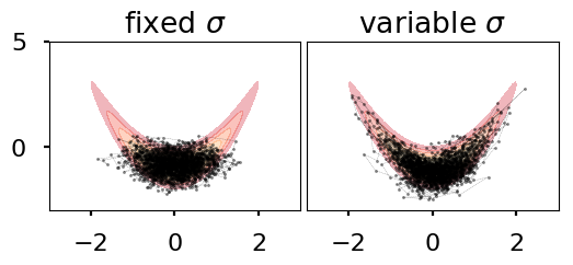
Two choices of diffusion coefficient are considered: the first, where , yields a neural SDE that can be trained using the techniques of Li et al. 2020. For the second, we choose
| (24) |
with , and parameterize by a two-layered neural network with 64 hidden units. This SDE can only be trained using our method. After training, to emulate the application of these SDEs as approximate samplers, a single sample path with 10,000 steps was simulated for each model using the Euler–Maruyama method. The resulting paths are compared in Figure 2. From data alone, both models constructed recurrent processes. The addition of a trainable diffusion coefficient led to improved adaptation of the sampler to the underlying curvature.
4.1.2 Visualizing regularization
As discussed in Liu et al. 2019, the stochastic noise injection in SDEs is a natural form of regularization, that can potentially improve robustness to noisy or adversarial data. We visualize this effect by considering the same stochastic normalizing flows treated in §4.1.1 with diffusion coefficient (24), and adjusting the parameter . Our data is generated in polar coordinates from a ten-pointed star-shaped distribution by
In Figure 3, we plot the densities for computed using Algorithm 1, noting that the case corresponds to a continuous normalizing flow. Increasing reveals generative models with expectedly higher variance, but with improved capacity to smooth out minor (potentially, unwanted) details.

4.2 Optimizing stochastic MCMC
An interesting class of SDE models for approximating a target distribution are targeted diffusions, solutions to SDEs that are -ergodic. A convenient representation of such diffusions are known (Ma et al. 2015). Because these diffusions are frequently used in MCMC algorithms, in a sense, conducting VI with respect to targeted diffusions is analogous to optimizing the convergence rate of stochastic MCMC algorithms.
To illustrate the potential applications of stochastic normalizing flows for finding and examining optimal stochastic MCMC algorithms for a particular target distribution, we consider a basic setup, where is the one-dimensional Cauchy distribution . All -ergodic SDEs are of the form
| (25) |
and we may choose arbitrarily. A priori, an optimal choice of (up to constants) to ensure rapid mixing of (25) does not appear obvious. The present rule of thumb from second-order methods takes (Girolami & Calderhead 2011). We train a stochastic normalizing flow for (25) with parameterized by a four-layer neural network with 32 hidden units in each layer. The corresponding loss function is taken to be the Kullback-Leibler divergence , estimated using Algorithm 1, with an penalty term over the weights of the neural network, to prevent taking . The results are presented in Figure 4.
Curiously, after training, we found the apparent “optimal” choice is approximately , where is the density of the standard normal distribution.
5 Conclusion
We have extended the continuous normalizing flows framework to generative models involving SDEs. Justified by rough path theory, our framework enables practitioners of neural ODEs to apply their existing implementation for training neural SDEs. This is advantageous, as neural SDEs have been suggested to be more robust than neural ODEs in high-dimensional real-world examples (Liu et al. 2019; Li et al. 2020). Stochastic normalizing flows can be implemented as a device for investigating “optimal” hyperparameters in stochastic MCMC, which could prove useful for informing future research, but they may require implementational improvements for high-dimensional cases, e.g., variance reduction techniques and improved loss estimators.
Acknowledgements.
We would like to acknowledge DARPA, NSF, and ONR for providing partial support of this work.
References
- Beskos et al. (2006) Beskos, A., Papaspiliopoulos, O., Roberts, G. O., and Fearnhead, P. Exact and computationally efficient likelihood-based estimation for discretely observed diffusion processes. Journal of the Royal Statistical Society: Series B (Statistical Methodology), 68(3):333–382, 2006.
- Chen et al. (2018) Chen, T. Q., Rubanova, Y., Bettencourt, J., and Duvenaud, D. K. Neural ordinary differential equations. In Advances in Neural Information Processing Systems, pp. 6571–6583, 2018.
- Davie (2008) Davie, A. M. Differential equations driven by rough paths: an approach via discrete approximation. Applied Mathematics Research eXpress, 2008, 2008.
- Dinh et al. (2015) Dinh, L., Krueger, D., and Bengio, Y. NICE: Non-linear independent components estimation. In Proceedings of the 3rd International Conference on Learning Representations (ICLR), 2015.
- Duchi et al. (2011) Duchi, J., Hazan, E., and Singer, Y. Adaptive subgradient methods for online learning and stochastic optimization. Journal of Machine Learning Research, 12:2121–2159, 2011.
- Dupont et al. (2019) Dupont, E., Doucet, A., and Teh, Y. W. Augmented neural ODEs. In Advances in Neural Information Processing Systems, 2019.
- Evans (2012) Evans, L. C. An introduction to stochastic differential equations, volume 82. American Mathematical Society, 2012.
- Friz & Hairer (2014) Friz, P. and Hairer, M. A Course on Rough Paths. Springer International Publishing, 2014.
- Friz & Victoir (2010) Friz, P. K. and Victoir, N. B. Multidimensional stochastic processes as rough paths: theory and applications, volume 120. Cambridge University Press, 2010.
- Gholami et al. (2019) Gholami, A., Keutzer, K., and Biros, G. ANODE: Unconditionally Accurate Memory-Efficient Gradients for Neural ODEs. In Proceedings of the Twenty-Eighth International Joint Conference on Artificial Intelligence (IJCAI-19), 2019.
- Girolami & Calderhead (2011) Girolami, M. and Calderhead, B. Riemann manifold Langevin and Hamiltonian Monte Carlo methods. Journal of the Royal Statistical Society: Series B (Statistical Methodology), 73(2):123–214, 2011.
- Grathwohl et al. (2018) Grathwohl, W., Chen, R. T., Betterncourt, J., Sutskever, I., and Duvenaud, D. FFJORD: Free-form continuous dynamics for scalable reversible generative models. arXiv preprint arXiv:1810.01367, 2018.
- Hairer & Wanner (1996) Hairer, E. and Wanner, G. Solving Ordinary Differential Equations II, volume 14 of Springer Series in Computational Mathematics. Springer-Verlag Berlin Heidelberg, 1996.
- Hodgkinson et al. (2019) Hodgkinson, L., Salomone, R., and Roosta, F. Implicit Langevin algorithms for sampling from log-concave densities. arXiv preprint arXiv:1903.12322, 2019.
- Hurn et al. (2007) Hurn, A. S., Jeisman, J., and Lindsay, K. A. Seeing the wood for the trees: A critical evaluation of methods to estimate the parameters of stochastic differential equations. Journal of Financial Econometrics, 5(3):390–455, 2007.
- Jia & Benson (2019) Jia, J. and Benson, A. R. Neural Jump Stochastic Differential Equations. In Proceedings of the 33rd Conference on Neural Information Processing Systems (NeurIPS 2019), 2019.
- Kloeden & Platen (2013) Kloeden, P. E. and Platen, E. Numerical solution of stochastic differential equations, volume 23. Springer Science & Business Media, 2013.
- Li et al. (2020) Li, X., Wong, T.-K. L., Chen, R. T., and Duvenaud, D. Scalable gradients for stochastic differential equations. arXiv preprint arXiv:2001.01328, 2020.
- Liu & Feng (2016) Liu, Q. and Feng, Y. Two methods for wild variational inference. arXiv preprint arXiv:1612.00081, 2016.
- Liu et al. (2019) Liu, X., Si, S., Cao, Q., Kumar, S., and Hsieh, C.-J. Neural SDE: Stabilizing Neural ODE Networks with Stochastic Noise. arXiv preprint arXiv:1906.02355, 2019.
- Lu et al. (2017) Lu, Y., Zhong, A., Li, Q., and Dong, B. Beyond finite layer neural networks: Bridging deep architectures and numerical differential equations. arXiv preprint arXiv:1710.10121, 2017.
- Lyons (1998) Lyons, T. J. Differential equations driven by rough signals. Revista Matemática Iberoamericana, 14(2):215–310, 1998.
- Ma et al. (2015) Ma, Y.-A., Chen, T., and Fox, E. A complete recipe for stochastic gradient MCMC. In Advances in Neural Information Processing Systems, pp. 2917–2925, 2015.
- Peluchetti & Favaro (2019) Peluchetti, S. and Favaro, S. Infinitely deep neural networks as diffusion processes. arXiv preprint arXiv:1905.11065, 2019.
- Pontryagin (2018) Pontryagin, L. S. Mathematical theory of optimal processes. Routledge, 2018.
- Rezende & Mohamed (2015) Rezende, D. J. and Mohamed, S. Variational inference with normalizing flows. In Proceedings of the 32nd International Conference on Machine Learning, 2015.
- Rhee & Glynn (2015) Rhee, C.-h. and Glynn, P. W. Unbiased estimation with square root convergence for SDE models. Operations Research, 63(5):1026–1043, 2015.
- Rischard et al. (2018) Rischard, M., Jacob, P. E., and Pillai, N. Unbiased estimation of log normalizing constants with applications to Bayesian cross-validation. arXiv preprint arXiv:1810.01382, 2018.
- Roosta & Ascher (2015) Roosta, F. and Ascher, U. Improved bounds on sample size for implicit matrix trace estimators. Foundations of Computational Mathematics, 15(5):1187–1212, 2015.
- Ryder et al. (2018) Ryder, T., Golightly, A., McGough, A. S., and Prangle, D. Black-box variational inference for stochastic differential equations. arXiv preprint arXiv:1802.03335, 2018.
- Salimans et al. (2015) Salimans, T., Kingma, D., and Welling, M. Markov chain Monte Carlo and variational inference: Bridging the gap. In International Conference on Machine Learning, pp. 1218–1226, 2015.
- Titsias & Ruiz (2019) Titsias, M. K. and Ruiz, F. J. Unbiased implicit variational inference. In Proceedings of the 22nd International Conference on Artificial Intelligence and Statistics (AISTATS), 2019.
- Twardowska (1996) Twardowska, K. Wong-Zakai approximations for stochastic differential equations. Acta Applicandae Mathematica, 43(3):317–359, 1996.
- Tzen & Raginsky (2019) Tzen, B. and Raginsky, M. Neural Stochastic Differential Equations: Deep Latent Gaussian Models in the Diffusion Limit. arXiv preprint arXiv:1905.09883, 2019.
- van den Berg et al. (2018) van den Berg, R., Hasenclever, L., Tomczak, J., and Welling, M. Sylvester normalizing flows for variational inference. In Proceedings of the Conference on Uncertainty in Artificial Intelligence (UAI), 2018.
- Wolf et al. (2016) Wolf, C., Karl, M., and van der Smagt, P. Variational inference with Hamiltonian Monte Carlo. arXiv preprint arXiv:1609.08203, 2016.
- Wong & Zakai (1965) Wong, E. and Zakai, M. On the convergence of ordinary integrals to stochastic integrals. The Annals of Mathematical Statistics, 36(5):1560–1564, 1965.
- Xu et al. (2019) Xu, M., Quiroz, M., Kohn, R., and Sisson, S. A. Variance reduction properties of the reparameterization trick. In The 22nd International Conference on Artificial Intelligence and Statistics, pp. 2711–2720, 2019.
- Yin & Zhou (2018) Yin, M. and Zhou, M. Semi-implicit variational inference. In Proceedings of the 35th International Conference on Machine Learning, 2018.
- Young (1936) Young, L. C. An inequality of the Hölder type, connected with Stieltjes integration. Acta Mathematica, 67:251–282, 1936.
- Zhang et al. (2019) Zhang, T., Yao, Z., Gholami, A., Keutzer, K., Gonzalez, J., Biros, G., and Mahoney, M. W. ANODEV2: A Coupled Neural ODE Evolution Framework. Advances in Neural Information Processing Systems, 2019.