Multiple Chemodynamic Stellar Populations of the Ursa Minor Dwarf Spheroidal GalaxyThanks: The data presented herein were obtained at the W.M. Keck Observatory, which is operated as a scientific partnership among the California Institute of Technology, the University of California and the National Aeronautics and Space Administration. The Observatory was made possible by the generous financial support of the W.M. Keck Foundation.2020Multiple Chemodynamic Stellar Populations of the Ursa Minor Dwarf Spheroidal Galaxy–References

Spectroscopic observations were carried out February 22–23 2009 (Kirby et al. 2010, first presented by), May 11–12 2010 (Kirby et al. 2018, first presented by), and April 20–22 2012 (not previously published) on the Keck/DEIMOS spectrograph (Faber et al. 2003). All these observations used the 1200G diffraction grating, which has a groove spacing of 1200 mm^-1 and a blaze wavelength of 7760 Å. The grating was tilted such that the typical central wavelength of a spectrum was 7800 Å, and the typical wavelength range was about 2600 Å. In practice, the wavelength range for each spectrum varied by up to 300 Å depending on the location of the slit along the dispersion axis. The grating was used in first order, and higher orders were blocked with the OG550 filter. DEIMOS has a flexure compensation system that keeps the wavelength calibration stable to within $\sim 0.1$ Å over a full night. The spectral resolution is $\Delta(\lambda)\sim 1.2$ Å, which translates to $R\sim 7000$ at the Ca triplet around 8500 Å.

Spectroscopic targets were selected from various photometric catalogs. Where the slitmask design constraints forced a choice among multiple candidates, we prioritized stars on the red giant branch (RGB). Kirby et al. 2010 described the slitmask design for the 2009 observations. Targets were selected from Bellazzini et al. 2002’s (Bellazzini et al. 2002) photometric catalog in the $V$ and $I$ filters. We used the color–magnitude diagram (CMD) in conjunction with Yonsei-Yale isochrones (Demarque et al. 2004) to inform the selection. Targets were selected between a blue bound and red bound. The blue bound was 0.1 mag bluer in de-reddened $(V-I)_{0}$ than a 2 Gyr isochrone with ${\rm[Fe/H]}=-3.76$ and ${\rm[\alpha/Fe]}=0.0$. The red bound was a 14 Gyr isochrones with ${\rm[Fe/H]}=+0.05$ and ${\rm[\alpha/Fe]}=+0.3$. Horizontal branch (HB) stars were also selected from a box in the CMD: $20.5>I_{0}>19.0$ and $-0.20<(V-I)_{0}<0.65$. Brighter stars were given higher priority.

Slitmasks from the 2010 observations were designed from SDSS $ugriz$ photometry (Abazajian et al. 2009). Stars were selected to lie within a color range around a 14.1 Gyr, ${\rm[Fe/H]}=-1.63$, Padova isochrone (Girardi et al. 2004). The allowed range was 0.4 mag bluer and 0.3 mag redder in $(g-r)_{0}$ color. We also selected HB stars from a box in the CMD: $21>r_{0}>20$ and $-0.4<(g-r)_{0}<0.0$. As for the 2009 observations, brighter stars were given higher priorities for spectroscopic selection.

Because there is no published photometric data set for Ursa Minor that covers the full extent of the galaxy and is sufficiently deep for our purposes, the spectroscopic target selection for the 2012 observing run relied on a number of different sources.

UMi has been observed by the Sloan Digital Sky Survey (SDSS), but the SDSS DR7 (Abazajian et al. 2009) coverage nearly bisects the galaxy along its major axis, with the southeast half of the galaxy included but no data in the northwest half. SDSS DR8 (Aihara et al. 2011a), in contrast, contains several stripes crossing the galaxy from southeast to northwest, with $\sim 20′$ gaps between each stripe. The difference in coverage between DR7 and DR8 is a result of different data quality criteria in the SDSS processing of those data sets (N. Padmanabhan 2012, private communication), but there is no evidence for systematic photometric errors in either the DR7 or DR8 imaging in this region. We therefore generated a combined SDSS DR7 + DR8 catalog for UMi, using DR7 measurements where available and DR8 elsewhere.¹¹ 1 DR8 contained an astrometry error of up to 0.25″ for northern targets (Aihara et al. 2011b; Ahn et al. 2012), so for stars in the DR8 photometric catalog we used the corrected positions provided in the early release of DR9 (Ahn et al. 2012).

In addition to SDSS, we used the wide-field Washington/DDO51 photometry of Palma et al. 2003, the deeper VI imaging of Bellazzini et al. 2002 in the center of the galaxy, and deep, wide-field gr imaging covering 1 deg² with CFHT/Megacam from Muñoz et al. 2018a. These catalogs were merged with the SDSS data taking precedence, followed by stars in the Palma, Bellazzini, and Muñoz catalogs, in that order. For the latter three data sets, we applied zero point offsets to the astrometry so that the median position differences with respect to SDSS DR9 of all stars in common were zero.

Spectroscopic targeting priorities for stars in the SDSS, Bellazzini, and Muñoz data sets were determined using ${\rm[Fe/H]}=-2$, 10 Gyr isochrones from Dotter et al. 2008. The RGB selection window was defined so as to include all obvious members of UMi near the center of the galaxy, with more generous color limits to the blue side of the RGB to allow for unusually metal-poor stars. We constructed a similar selection window for horizontal branch (HB) stars by generating a large number of synthetic HB stars with the online code provided by Dotter et al. 2007 using the same age and metallicity as for the RGB and then fitting a polynomial to determine the luminosity of the HB as a function of color. We assigned RGB candidates higher priorities than HB candidates, with relative priorities determined by magnitude within each category (where preference is given to brighter stars), and then added priority bonuses for stars already confirmed to be UMi members by Palma et al. 2003 or the 2009/2010 Kirby data sets described above. Stars located within the bounds of either of the two possible substructures in UMi identified by Pace et al. 2014 were given the highest priorities, and then slitmasks were placed to ensure full coverage of both substructures.

We reduced the DEIMOS data using the spec2d pipeline developed by the DEEP2 team (Cooper et al. 2012; Newman et al. 2013). The pipeline cuts out the spectrally dispersed image of each slit from the raw data. The image is flat fielded, and a two-dimensional wavelength solution is calculated from an exposure of Kr, Ne, Ar, and Xe arc lamps. The typical root mean square difference between the known arc line wavelengths and the calculated wavelength solution is 0.015 Å ($0.5\,\mathrm{km}\,\mathrm{s}^{-1}$). The stellar spectrum is extracted with “optimal” extraction (Horne 1986) and made into a sky-subtracted, wavelength-calibrated, one-dimensional spectrum. We made some improvements to the pipeline appropriate for our purposes. For example, the procedure for defining the extraction window was optimized for extracting unresolved stars rather than extended galaxies (Simon & Geha 2007). The one-dimensional wavelength arrays were modified with slight offsets in order to align sky emission lines with their known wavelengths. The wavelength arrays were also modified to remove the effect of differential atmospheric refraction perpendicular to the slit.

We measured radial velocities for each star by comparing the spectra with a set of template spectra measured with DEIMOS (Kirby et al. 2015, observed by). The velocities were calculated from the wavelength shift in log space that minimized $\chi^{2}$ between the target and template spectra. This procedure is similar to a cross-correlation (Tonry & Davis 1979), but it also takes into account variance in the observed spectrum.

We checked each radial velocity measurement by plotting the template spectrum on top of the target spectrum shifted into the rest frame. In several cases, the velocity measurement clearly failed, and the spectra did not line up. The typical cause was an artifact at the edge of the target spectrum. In these cases, we masked out the offending region of the spectrum and repeated the velocity measurement.

Because DEIMOS is a slit spectrograph, mis-centering of stars can cause spurious offsets in the wavelength solution, which translate into offsets in the measured radial velocity. We treated this offset as a shift in the zeropoint of the radial velocity. We measured the zeropoint by using the observed wavelengths of telluric absoprtion from the Earth’s atmosphere, which should be at rest in the geocentric frame. This is sometimes known as the “A-band correction” (Sohn et al. 2007). We cross-correlated each of the observed spectra with the spectrum of a hot star observed with DEIMOS by Kirby et al. 2015. The velocity zeropoint was taken to be the velocity shift required to align the template spectrum with the telluric absorption features. This zeropoint was added to the radial velocity measured from the stellar absorption lines. We inspected each spectrum to ensure that the telluric cross-correlation was valid, just as we did for the stellar absorption. In about a dozen cases where the DEIMOS chip gap fell in the A-band, we had to re-evaluate the telluric cross-correlation after excluding some pixels around the chip gap.

We calculated velocity errors by resampling the target spectrum 1000 times. In each Monte Carlo trial, we constructed a new spectrum by perturbing the original flux value. The magnitude of the perturbation was sampled from a Gaussian random distribution with a variance equal to the variance estimated for that pixel by spec2d. The velocity error was equal to the standard deviation of all of the Monte Carlo trials. Simon & Geha 2007 found from repeat measurements of the same stars that this statistical error was an incomplete description of the total error. Following their example, we calculated the total error by adding a systematic error of 2.2 km s^-1 in quadrature with the Monte Carlo statistical error.

We measured metallicities by comparing the continuum-normalized observed spectra to a grid of synthetic spectra. This procedure is identical to that of Kirby et al. 2008; Kirby et al. 2010. We started with a guess at the effective temperature, surface gravity, and metallicity of the star by combining the stars’ colors and magnitudes with theoretical isochrones. The temperature and metallicity were allowed to vary to minimize $\chi^{2}$ between the observed spectrum and the synthetic grid. Our measured value of [Fe/H]²² 2 ${\rm[Fe/H]}=\log\frac{n({\rm Fe})/n({\rm H})}{n_{☉}({\rm Fe})/n_{☉}({\rm H})}$ where $n$ is atomic number density. is the one that minimized $\chi^{2}$.

Errors on [Fe/H] were estimated from the diagonal terms of the covariance matrix. This is an incomplete estimate of the error, largely due to covariance with temperature. Kirby et al. 2010 found that adding a systematic error of 0.11 dex in quadrature with the statistical error is an adequate estimate of the error. We adopted the same approach.

Our Keck/DEIMOS measurements are listed in Table 2.

To verify our measurements we examined stars with repeated measurements (using a cross-match radius of 1″). We find 155 stars with two spectral measurements and 12 stars with three measurements. In Figure 1, we compare the repeated line-of-sight velocity and metallicity measurements. We compute the normalized difference, $\Delta$, between measurements. For radial velocity measurements, $\Delta_{v}=(v_{1}-v_{2})/\sqrt{\sigma_{\epsilon,v,1}^{2}+\sigma_{\epsilon,v,2}^{2}}$, where $v$ and $\sigma_{\epsilon,v}$ correspond to the radial velocity and velocity error, respectively. If the repeated measurements are consistent, the $\Delta$ distribution will follow a Gaussian distribution with a mean of zero and variance of unity. Based on a Shapiro-Wilk test we find that our repeat measurements are consistent with a Gaussian distribution ($p=0.34$). After removing stars with clear velocity variation we find, $\overline{\Delta_{v}}=0.24$ and $\sigma_{\Delta_{v}}=1.18$ for repeated velocity measurements and $\overline{\Delta_{v}}=-0.15$ and $\sigma_{\Delta_{v}}=1.00$ for repeated metallicity measurements. The second and fourth panels of Figure 1 show $\Delta$ for the velocity and metallicity measurements, respectively. The tails in the velocity distribution could be due to unresolved binary stars.

To combine velocity measurements we use the weighted mean as the combined radial velocity. For the error we compute the variance of the weighted mean and weighted standard deviation and take the larger of the two for the combined velocity error. When the weighted standard deviation is larger than the variance of the weighted mean, the star may be variable in velocity and we use the weighted standard deviation to be conservative. For metallicity measurements we use the weighted mean and variance of the weighted mean for all combined measurements.

We compare our velocity and metallicity measurements to two other large UMi spectroscopic samples (Figure 2). Muñoz et al. 2005 presented velocity measurements from a combination of Keck/HIRES and WHT/WYFFOS (Wilkinson et al. 2004, the latter were originally presented in). Previous analysis of this data set motivated our target selection (Pace et al. 2014). Spencer et al. 2018 utilized MMT/Hectochelle to measure velocities and metallicities in UMi. There are 108 and 277 stars in common with our data set and Muñoz et al. 2005 and Spencer et al. 2018, respectively. Overall, we find that our velocities are offset from both studies; the average mean normalized offset (after removing outliers) is $\overline{\Delta_{v}}=0.70$, $\sigma_{\Delta_{v}}=1.17$ and $\overline{\Delta_{v}}=0.77$, $\sigma_{\Delta_{v}}=0.92$ for Muñoz et al. 2005 and Spencer et al. 2018, respectively. These offsets are likely caused by zero-point offsets in the radial velocity templates assumed between different analyses. We find that there is an offset in the metallicity between the Spencer et al. 2018 MMT/Hectochelle measurements and find $\overline{\Delta_{\rm[Fe/H]}}=-0.98$ and $\sigma_{\Delta_{\rm[Fe/H]}}=1.03$. This offset may be due to the differences in measurement techniques or due to the different spectral ranges and resolutions. Based on our UMi analysis, we find these normalized offsets translate to offsets of $\Delta\overline{v}\approx 2.4\,\mathrm{km}\,\mathrm{s}^{-1}$ and $\Delta\overline{\rm[Fe/H]}\approx 0.16$. While there are offsets between the different studies, we find that the errors are consistent between the different studies.

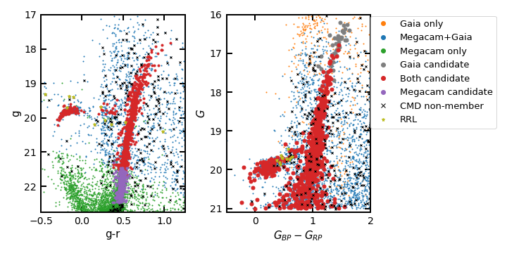
As mentioned in Section 2.1, at the time of our target selection and observations there was not a deep and wide-field public photometric catalog for UMi. There are now several, including the wide-field CFHT/Megacam data (Muñoz et al. 2018a), Pan-STARRS1 (Chambers et al. 2016), and Gaia DR2 (Gaia Collaboration et al. 2018a). We use the gr CFHT/Megacam photometry (Muñoz et al. 2018a) for the majority of the sample and Gaia DR2 photometry ($G$ and $G_{\rm BP}-G_{\rm RP}$) for the brightest stars in the sample that are saturated in the Megacam catalog ($G<18$, roughly $g\sim 18.75$). We perform a broad isochrone selection to pick stars with colors and magnitudes consistent with UMi. For the Gaia DR2 photometry, we base on cuts on the selection by Gaia Collaboration et al. 2018b. For the Megacam photometry and stars on the red giant branch, we select stars within a color window of 0.12 mag from an ${\rm[Fe/H]}=-2$, 10 Gyr isochrone (Dotter et al. 2008) and exclude stars fainter than $g=22.5$. For the horizontal branch selection, we select stars within magnitude windows of 0.3 mag and 0.2 mag for stars with $g-r<0$ and $0<g-r<0.55$ respectively. The window in the red horizontal branch region is narrower due to the increase in MW interlopers. This selection is similar to the target selection on the preliminary Megacam photometry.

We use Gaia DR2 proper motions to improve MW foreground identification and determine the proper motion of UMi. We cross match our spectroscopic sample with the Gaia DR2 catalog with a cross-match radius of 1″ (for most stars the cross-match radius is less than 0$\aas@@fstack{\prime\prime}$5) and find 1060 matches out of 1532 stars with an astrometric solution (astrometric_params_solved=31). We utilize the stellar parallax to identify nearby disk stars. We consider all stars with a non-zero parallax as members of the MW disk ($\varpi-3\sigma_{\varpi}>0$). We calculate the tangential velocity for each star assuming it is at the distance to UMi (Table 3). Any star that would be unbound at UMi’s distance ($v_{\rm tan}-3\sigma_{v_{\rm tan}}>v_{\rm escape}$) is considered a nearby MW foreground star (Pace & Li 2019).

RR Lyrae stars are variable in velocity and not suited for kinematic analysis. We cross-match our sample to the Pan-STARRS RR Lyrae (Sesar et al. 2017) and Gaia DR2 RR Lyrae catalogs (Clementini et al. 2019) and find 17 and 15 matches, respectively (with a 0$\aas@@fstack{\prime\prime}$5 cross-match radius). We find a total of 18 RR Lyrae in our spectroscopic sample as 12 stars overlap between the RR Lyrae catalogs. The velocities and locations on a color-magnitude diagram of all 18 stars are consistent with membership in UMi. Two RR Lyrae each have two velocity measurements and exhibit clear velocity variation (Gaia source_id, 1645449593695899264: $-298.3\pm 2.5$ and $-279.3\pm 2.4$ and 1645468079235094784: $-229.6\pm 2.6$ and $-235.7\pm 2.5$). We exclude all known RR Lyrae from our analysis.

We use the surface gravity sensitive spectral feature at Na I at 8190 Å  to identify additional MW foreground stars (Spinrad & Taylor 1971; Cohen 1978). Stars with $\sigma_{\epsilon,v}>20\,\mathrm{km}\,\mathrm{s}^{-1}$ are excluded and we do not use the metallicity measurements for stars with $\sigma_{\epsilon,{\rm[Fe/H]}}>0.5$ dex. We compute the $\chi^{2}$ of a non-variable velocity for each star (i.e., any variation is due just to measurement errors) and the corresponding p-value. We exclude seven stars with clear indications of velocity variability from our analysis ($\Delta_{v}>3$ and/or $p<0.01$). After our color-magnitude selection and removing stars with indications of variability we have 1009 candidate UMi stars. Based on the parallax, large proper motion, or Na I doublet, 64 of these stars are immediately identified as MW foreground stars.

Due to limited telescope time, not all spectroscopic candidates can be observed. The spatial distribution of stars with spectroscopic measurements generally does not follow the intrinsic spatial distribution of stars (due to telescope field-of-view, mask size, etc). To ensure that spatial parameters of the dSph can be recovered from the spectroscopic distribution we compute the selection function, $S(x,y)$. The selection function acts as a mapping between the observed and intrinsic spatial distribution of stars (Wang et al. 2005; Walker & Peñarrubia 2011).

To construct $S(x,y)$, we smooth the ratio of observed to candidate stars within the UMi region (Walker & Peñarrubia 2011):

To set $k$, we construct and observe mock data sets with different values of $k$ ranging from 25 to 400 parsecs (1$′$ to 18$′$ at $d=76$ kpc). We find, that for spherically symmetric systems, the choice of $k$, does not make an appreciable difference³³ 3 Walker & Peñarrubia 2011 reach the same conclusion.. Whereas, for axisymmetric systems, an incorrect choice in $k$ will strongly bias the recovered structural parameters. Our tests, with a layout approximating the locations and sizes of Keck/DEIMOS masks, show that $50\,\mathrm{pc}\leq k\leq 75\,\mathrm{pc}$ ($2′\leq k\leq 3′$) correctly recovers the input structural parameters. A larger choice of $k$ will bias the structural posteriors. The spatial scale will be underestimated and axis ratio overestimated. The spatial bias increases as $k$ increases.

In Figure 4, we plot the selection function we use for the UMi analysis with $k=50$ pc. We align the x-axis and the major axis (Muñoz et al. 2018b, using a position angle of $\theta=50\degree$). We fix $k=50$ pc for the main analysis.

This analysis uses line-of-sight velocity ($v$, $\sigma_{\epsilon,v}$), metallicity (${\rm[Fe/H]}$, $\sigma_{\epsilon,\rm[Fe/H]}$), spatial position ($x$, $y$), and proper motion⁴⁴ 4 $\mu_{\alpha*}=\mu_{\alpha}\cos{\delta}=-\mu_{W}$ ($\mu_{\alpha*}$, $\sigma_{\epsilon,\mu_{\alpha}*}$, $\mu_{\delta}$, $\sigma_{\epsilon,\mu_{\delta}}$, $C_{\mu_{\alpha*}\times\mu_{\delta}}$) for each data point⁵⁵ 5 We note that not all stars have metallicity or proper motion measurements. For each data point without a particular measurement, that likelihood term must be integrated out (i.e. all possible metallicity or proper motion values are considered). As the individual likelihood terms are normalized to unity, integrating over all possible values drops the term from the likelihood and the membership probability for that star will only consider spatial and velocity information. . Our analysis utilizes synthetic measurements of the iron abundance, [Fe/H]. Other works have utilized different metallicity tracers, for example, the Ca ii triplet (Battaglia et al. 2008), or the $\Sigma$Mg index (Walker & Peñarrubia 2011).

We assume that probability distributions of the velocity, position, metallicity, and proper motions are independent of one another, therefore, the likelihood of the dSph or MW is,

The majority of the probability distributions are assumed to be Gaussian or multivariate Gaussian distributions. For example, the probability distribution of the velocity term is: $\mathcal{P}^{{\rm vel}}({v_{i},\sigma_{\epsilon,v}}_{i}|\overline{v},\sigma_{v})=\mathcal{N}(v_{i}-\overline{v},\sqrt{\sigma_{\epsilon,v,i}^{2}+\sigma_{v}^{2}})$, where $\mathcal{N}(a,b)$ is a normal distribution where the mean, a, and dispersion, b. $\overline{v}$ and $\sigma_{v}$ are the average velocity and velocity dispersion, respectively.

For an extended object, like a dSph, the average velocity is a function of spatial position due to projection effects, sometimes referred to as the perspective motion, and we replace $\overline{v}$ with $v_{\rm rel}(\alpha,\delta)$ (Feast et al. 1961; van der Marel et al. 2002; Kaplinghat & Strigari 2008; Walker et al. 2008). The effect can be understood as the difference between the $z$ coordinate and line-of-sight direction, for example, $v_{\rm rel}(x,y)\approx-v_{z}+v_{x}x/d+v_{y}y/d$ (Kaplinghat & Strigari 2008). Our implementation of the perspective motion follows the appendix of Walker et al. 2008. For UMi, the effect is $\Delta\lvert v\rvert\sim 0.1-0.2\,\mathrm{km}\,\mathrm{s}^{-1}$.

The bright dSphs have flat isothermal line-of-sight velocity dispersions (Muñoz et al. 2005; Muñoz et al. 2006; Walker et al. 2007), therefore we initially assume $\sigma_{v}$ is constant with radius. However, this assumption may not hold for individual chemodynamic components (Battaglia et al. 2008; Strigari et al. 2017); we address this in Section 4. We assume the metallicity likelihood is a Gaussian distribution with a free mean, $\overline{\rm[Fe/H]}$ and dispersion, $\sigma_{\rm[Fe/H]}$.

The likelihood for the spatial distribution is (Wang et al. 2005; Walker & Peñarrubia 2011),

We model the proper motion likelihood as a multivariate Gaussian due to the correlated error between the $\mu_{\alpha*}$ and $\mu_{\delta}$ components (Pace & Li 2019). The proper motion likelihoods have free means, $\overline{\mu_{\alpha*}}$ and $\overline{\mu_{\delta}}$, and dispersions, $\sigma_{\mu_{\alpha*}}$ and $\sigma_{\mu_{\delta}}$. For the dSph component we fix $\sigma_{\mu_{\alpha*}}=\sigma_{\mu_{\delta}}=10\,\mathrm{km}\,\mathrm{s}^{-1}=0.03\,{\rm mas\,yr^{-1}}$ and leave the MW dispersions as free parameters. The proper motion errors for the brightest UMi stars are $\approx 40\,\mathrm{km}\,\mathrm{s}^{-1}$ and rapidly increase for fainter stars. Due to the large errors it is not possible to infer the intrinsic dSph proper motion dispersions but this may be possible in future Gaia data releases. The expected MW halo dispersion will be $\approx 100-200\,\mathrm{km}\,\mathrm{s}^{-1}$ depending on the component (e.g., disk, halo).

The individual MW probability distributions are similar to the dSph components. We assume Gaussian or multivariate Gaussians for the velocity, metallicity, and proper motion components with free means ($\overline{v}_{\rm MW}$, $\overline{\rm[Fe/H]}_{\rm MW}$, $\overline{\mu_{\alpha*,\,{\rm MW}}}$, $\overline{\mu_{\delta,\,{\rm MW}}}$) and variances ($\sigma_{v,\,{\rm MW}}$, $\sigma_{\rm[Fe/H],\,MW}$, $\sigma_{\mu_{\alpha*},\,{\rm MW}}$, $\sigma_{\mu_{\delta},\,{\rm MW}}$). For the spatial distribution we assume that it is uniform within the UMi region. After accounting for the selection function the spatial probability distribution is: $\mathcal{P}^{{\rm spatial}}_{\rm MW}(x_{i},y_{i})=S(x_{i},y_{i})/\int S(x,y)dA$.

There are a number of stars that can be immediately identified as foreground stars due to the surface gravity sensitive spectral feature at Na I at 8190 Å , a non-zero parallax, and/or an extremely large tangential velocity (see Section 2.4). We do not want to immediately remove these stars from the sample as their $v$ and $\mathrm{[Fe/H]}$ will help construct the MW foreground distribution and assist in identifying MW stars without Gaia astrometric measurements. These stars are only used in the MW likelihood and we do not include their proper motion information in the likelihood.

We first explore a model with a single dSph component to identify UMi and foreground MW stars. The center, position angle, and distance are fixed to literature measurements and the adopted values are listed in Table 3. There are 1009 stars that pass our cuts and are used as input in the mixture model. Stars identified as MW stars based on their parallax, Na I doublet, or large proper motions are fixed to the MW component and only their velocity and metallicity information is included in the mixture model.

We find $\overline{v}=-244.7\pm 0.3\,\mathrm{km}\,\mathrm{s}^{-1}$ and $\sigma_{v}=8.7\pm 0.3\,\mathrm{km}\,\mathrm{s}^{-1}$ for UMi. The velocity dispersion is consistent with $\sigma_{v}=9.5\pm 1.2\,\mathrm{km}\,\mathrm{s}^{-1}$ (Walker et al. 2009) and in between the measurements of $\sigma_{v}=8.0\pm 0.3\,\mathrm{km}\,\mathrm{s}^{-1}$ (Spencer et al. 2018)⁶⁶ 6 We note that in our analysis of the Spencer et al. 2018 data, we find a larger $\sigma_{v}$ value that is consistent with our Keck/DEIMOS results. For further details see Section 4.3. and $\sigma_{v}=11.5\pm 0.6$ (Muñoz et al. 2005). The Muñoz et al. 2005 data set is more spatially extended and is a combination of WHT/WYFFOS (Wilkinson et al. 2004) and Keck/HIRES observations. The difference in $\sigma_{v}$ could be due to a $\sigma_{v}$ that increases with radius, or the Muñoz et al. 2005 data set could consist of a larger fraction of stars in the kinematically hotter population (see next section). Another possibility is a velocity offset between the two instruments which inflates $\sigma_{v}$. The metallicity properties we find are $\overline{\mathrm{[Fe/H]}}=-2.13\pm 0.02$ and $\sigma_{\mathrm{[Fe/H]}}=0.35\pm 0.01$ which agrees with $\overline{\mathrm{[Fe/H]}}=-2.13\pm 0.01$ and $\sigma_{\mathrm{[Fe/H]}}=0.34$ from Kirby et al. 2011. The spatial properties we derive assuming a Plummer distribution are $r_{{\rm p}}=447_{-20}^{+23}\,{\rm pc}$, $\epsilon=0.59\pm 0.02$, and $R_{\rm h}=287_{-10}^{+11}\,{\rm pc}$ ($R_{h}=r_{p}\sqrt{1-\epsilon}$). This agrees with $q=0.45\pm 0.01$ and $R_{h}=271\pm 3\,{\rm pc}$ derived from deep, wide-field photometric data (Muñoz et al. 2018b). Our proper motion measurement agrees within the errors with previous Gaia DR2 measurements (Gaia Collaboration et al. 2018b; Fritz et al. 2018).

Of the 1009 candidate stars, 892 (898) have membership greater than $>0.95$ ($>0.90$). The inclusion of Gaia proper motions results in very few stars with intermediate membership; only 12 stars have membership values in the range $0.05<p_{\rm dSph}<0.90$ (only one of which has a Gaia DR2 astrometric solution). Overall, we find our metallicity, spatial, and proper motion properties of UMi are consistent with previous work whereas our velocity dispersion measurement is in moderate tension ( $\sim 2-3\sigma$) with both Muñoz et al. 2005 and Spencer et al. 2018 but lies in between these measurements.

In our search for multiple chemodynamic populations, we use RGB UMi members with metallicity measurements ($N=679$; $p_{\rm dSph}>0.95$). Metallicity measurements are key for this analysis and horizontal branch stars may not have as robust metallicity measurements. To separate the populations, we set a prior between the velocity dispersions ($\sigma_{v,1}<\sigma_{v,2}$) and do not assume any additional priors between the metallicity and/or spatial parameters. We assume there is no offset in mean line-of-sight velocity or proper motion between the two populations. The posteriors of the two population analysis are listed in Table 4 along with results from single component analysis with the same subset of RGB stars.

We find, with high significance ($\ln{B}=33.47$), two populations with distinct chemical, kinematic, and spatial distributions. The first population is kinematically cold ($\sigma_{v}=4.9_{-1.0}^{+0.8}\,\mathrm{km}\,\mathrm{s}^{-1}$), more metal-rich ($\overline{\mathrm{[Fe/H]}}=-2.05\pm 0.03$), and centrally concentrated, ($R_{h}=221_{-17}^{+17}\,{\rm pc}$). The second population is kinematically hot ($\sigma_{v}=11.5_{-0.8}^{+0.9}\,\mathrm{km}\,\mathrm{s}^{-1}$), more metal-poor ($\overline{\mathrm{[Fe/H]}}=-2.29_{-0.06}^{+0.05}$) and spatially more extended ($R_{h}=374_{-37}^{+49}\,{\rm pc}$). The chemodynamical ordering of the two populations is the same as other dSphs (Battaglia et al. 2008, e.g., Sculptor;) despite only imposing a prior on $\sigma_{v}$. Although the metallicity separation is less than found in other dSphs, we will refer to the two stellar populations as the metal-rich and metal-poor populations. While the metallicity distributions overlap, the two stellar populations have distinct velocity, metallicity, and spatial distributions.

We show the spatial distribution of stars in each population in Figure 5. Interestingly, the metal-rich population is significantly more flattened ($\epsilon=0.75\pm 0.03$) than the metal-poor population ($\epsilon=0.33_{-0.12}^{+0.09}$) and UMi in general ($\epsilon=0.55\pm 0.01$). Both populations have major axes of similar length. In our standard analysis, we fixed the position angle. We have explored varying the position angle for each component and find that the difference in position angle between the two populations is small, $\Delta\theta<5\degree$. The visual offset in Figure 5 is due to the spectroscopic selection. While we account for the spectroscopic selection function it is possible that there is a remaining bias. In Section 4.3 we examine and confirm the flattened metal-rich component with an independent UMi spectroscopic data set.

In Figure 6, we examine the radial dependence of the average metallicity and metallicity dispersion of both populations. The two populations are clearly offset in mean metallicity in all radial bins. The difference in metallicity between the two populations is less than the differences observed in other dSphs (e.g., Fornax, Sculptor). The metallicity dispersion is larger in the metal-poor population compared to the metal-rich population.

Figure 7 shows the radial dependence of $\sigma_{v}$ of the metal-rich and metal-poor populations. The metal-rich $\sigma_{v}$ is constant with radius whereas the metal-poor $\sigma$ has hints that it deceases from $\approx 13\,\mathrm{km}\,\mathrm{s}^{-1}$ at the center to $\approx 10\,\mathrm{km}\,\mathrm{s}^{-1}$ at large radii. For comparison, we also include the binned single-component velocity dispersion (black). Decreasing velocity dispersion profiles for sub-components are not unusual in a dSph. They have been observed in the Fornax metal-poor population (Amorisco & Evans 2012b) and in the Sculptor metal-rich population (Battaglia et al. 2008).

To test whether our assumption of a constant velocity dispersion affects the identification of stars within either chemodynamic population, we explore a model with a radial dependence. The velocity dispersion functional form we use is: $\sigma_{v}(R_{e})=\sigma_{o}\left(1+R_{e}/R_{\sigma}\right)^{\alpha}$ (we use the same ellipticity for the spatial distribution and dispersion function). This model has two additional parameters: a radial scale, $R_{\sigma}$, and a power law slope, $\alpha$. The priors for each parameter are $-2<\log_{10}{\left(R_{\sigma}/1\,{\rm kpc}\right)}<1$ and $-5<\alpha<5$. Overall, the inferred functional forms for the metal-rich and metal-poor are consistent with the binned profiles; the metal-rich population is constant with radius whereas the metal-poor population decreases with radius from $\approx 13\,\mathrm{km}\,\mathrm{s}^{-1}$ to $\approx 10\,\mathrm{km}\,\mathrm{s}^{-1}$. The posterior distribution for velocity dispersion parameters are degenerate with one another and non-kinematic parameters change little compared to the constant velocity dispersion model. We find little change in the assignment of stars to either population. The net absolute change ($\sum\Delta\lvert p_{\sigma(R_{e})}-p_{\rm const}\rvert$) is $\sim 24$ and the maximum absolute change of an individual star is small ($\Delta p_{i}=0.16$). The mean and median differences of the membership are both 0.03 and the standard deviation is 0.03. Assuming a constant velocity dispersion model does not affect the identification of two populations or parameter inference.

Our UMi sample is built from three different observing epochs with very different target selection criteria (a combination of different spatial regions and a different photometric input catalogs). To explore whether the inhomogeneous target selection is driving our inference of the chemodynamic populations we apply the same analysis on three subsets. Each subset excludes one of the three epochs and the subset excluding the 2009, 2010, and 2012 data contains 435, 554, and 302 stars, respectively. Applying the same analysis to each subset, we continue to identify two chemodynamic populations with high significance ($\ln{\rm B}=23.57,15.18,25.14$). Our inhomogeneous target selection does not affect the inference of two chemodynamic populations.

As a cross check, we search for and find two chemodynamic populations with the independent UMi spectroscopic survey from MMT/Hectochelle observations (Spencer et al. 2018). We first apply a similar mixture model to determine UMi membership and emphasize again that Gaia proper motions significantly improve dSph and foreground separation. The MMT sample contains brighter stars in general than the Keck sample and all but one star is in the Gaia DR2 catalog. We select candidate UMi stars with a rough color-magnitude diagram selection with Gaia photometry ($G_{BP}-G_{RP}$ vs G) based on a slightly expanded selection in Figure 3 of Gaia Collaboration et al. 2018b. Using proper motion, velocity, metallicity, and spatial positions we identify 413 stars as UMi members ($p_{\rm dSph}>0.95$). Similar to the Keck/DEIMOS data set, very few stars have intermediate membership; only 5 stars have a membership between $0.01<p_{\rm dSph}<0.95$.

The overall UMi properties⁷⁷ 7 The mean velocity and metallicity we find for the MMT data are offset from the Keck value by $\approx 2.3\,\mathrm{km}\,\mathrm{s}^{-1}$ and $\approx 0.13$, respectively. These are similar to the offsets found between common stars in Section 2.3. we find in this data set are similar to the Keck/DEIMOS data set: $\overline{v}=-246.9\pm 0.4\,\mathrm{km}\,\mathrm{s}^{-1}$, $\sigma_{v}=8.6\pm 0.3\,\mathrm{km}\,\mathrm{s}^{-1}$, $\overline{[{\rm Fe/H}]}=-2.02\pm 0.02$, $\sigma_{\rm[Fe/H]}=0.37\pm 0.02$, $r_{p}=450_{-30}^{+33}\,{\rm pc}$, $\epsilon=0.56\pm 0.03$, $R_{h}=297\pm 15\,{\rm pc}$. We find a $\sigma_{v}$ value that is $\approx 0.6\,\mathrm{km}\,\mathrm{s}^{-1}$ larger than Spencer et al. 2018. This difference is likely due to our use of Gaia DR2 astrometry and the different membership methods (mixture model versus $\sigma$ clipping).

We find statistically significant evidence for two chemodynamic populations in the MMT/Hectochelle data set ($\ln{B}=17.94$). The overall results are similar to the Keck/DEIMOS sample; the first population is centrally-concentrated, dynamically-cold, and metal-rich whereas the secondary component is more extended, kinematically-hot, and metal-poor. The properties of the two populations are summarized in the last two columns of Table 4. In table 5, we list our dSph and metal-rich membership for stars in the MMT sample. With the MMT data, we confirm the metal-rich population is aspherical ($\epsilon=0.64\pm 0.04$) while the extended population is more spherical ($\epsilon=0.21_{-0.14}^{+0.16}$, constrained to be $\epsilon<0.38$ at the 90% confidence interval). We note that the two populations are closer in velocity dispersion ($\Delta\sigma_{v}\sim 4.4\,\mathrm{km}\,\mathrm{s}^{-1}$) than our results in the Keck data set ($\Delta\sigma_{v}\sim 6.6\,\mathrm{km}\,\mathrm{s}^{-1}$). The MMT metal-poor $\sigma_{v}$ is consistent within errors with the Keck measurement whereas the metal-rich $\sigma_{v}$ is larger and disagrees at $\sim 2\sigma$. The metal-rich component is more metal-rich than the Keck results; this may be due to offset found between the samples based on repeated measurements (see Section 2.3 and Figure 2). The MMT metal-poor population is more extended but more uncertain compared to the Keck results (due to the overall lower number of stars). We find an overall smaller fraction of stars in the metal-poor population ($f=0.24$ versus $f=0.46$). The differences between the inferred properties may be based on differences in the target selection in the two data sets.

In Figure 8, we show the binned $\sigma_{v}$ profiles with the MMT data. The metal-poor $\sigma_{v}$ declines from $\approx 15\,\mathrm{km}\,\mathrm{s}^{-1}$ to $\approx 10\,\mathrm{km}\,\mathrm{s}^{-1}$ and the metal-rich population is constant with radius. This confirms the $\sigma_{v}$ profile of the metal-poor population that was seen in the Keck data.

The results from the MMT sample independently confirm the two chemodynamical populations in UMi. Moreover, it confirms two interesting features in UMi: a flattened metal-rich population with an almost spherical metal-poor component and a declining $\sigma_{v}$ profile for the metal-poor population. For the following analysis, we will analyze both UMi data sets independently. We opt not to combine the data sets due to the observed offsets in velocity and metallicity and the different methodologies for velocity and metallicity measurements.

The flattened nature of the metal-rich population is reminiscent of a disk galaxy and a natural question is whether it is rotating. We first search for rotation with a simple test, splitting the sample in half based on bisecting lines at different position angles and computing the difference between the mean velocity in each half. The entire Keck RGB data set and the Keck metal-rich population show little to no signal whereas the Keck metal-poor population has an amplitude of $\sim 2\,\mathrm{km}\,\mathrm{s}^{-1}$. In contrast, we observe a signal in the entire MMT data set, the MMT metal-rich population, and the MMT metal-poor population with amplitudes of $\sim 3$, $\sim 6$, and $\sim 2\,\mathrm{km}\,\mathrm{s}^{-1}$, respectively. In all cases with a signal, including the Keck metal-poor population, the peak amplitude occurs near the photometric minor axis corresponding to prolate rotation ($\theta=-40,140\degree$ corresponds to the photometric minor axis)⁸⁸ 8 The Muñoz et al. 2005 data set also shows evidence for rotation with an amplitude of $\sim 5\,\mathrm{km}\,\mathrm{s}^{-1}$ that peaks at a similar position angle.. We show the results of this test for the MMT data set in Figure 9. We note that this is one of the better examples of rotation in the subsets examined.

To further quantify any potential rotation signal, we explore a rotation model that is constant with radius. We add the rotation term to the relative velocity: $v_{\rm rel}=\overline{v}+A_{\rm rot}\cos{\left(\theta-\theta_{\rm rot}\right)}$ (Wheeler et al. 2017). This includes two additional parameters, an amplitude, $A_{\rm rot}$, and a rotation angle, $\theta_{\rm rot}$. In the Keck RGB data set, the rotation amplitudes we derive are consistent with zero and we find upper limits of $A_{\rm rot}<2.0\,{\rm kms^{-1}kpc^{-1}}$, $A_{\rm rot}<4.0\,{\rm kms^{-1}kpc^{-1}}$, and $A_{\rm rot}<2.2\,{\rm kms^{-1}kpc^{-1}}$ (upper limits are at 95% confidence) for the metal-rich population, metal-poor population, and the entire sample, respectively⁹⁹ 9 We have explored this test by adding rotation to one component at a time and both components simultaneously with similar results.. In the MMT data set, we measure rotation amplitudes and rotation axes of $A_{\rm rot}=1.9\pm 0.9\,{\rm kms^{-1}kpc^{-1}}$ and $\theta_{\rm rot}=156_{-17}^{+24}\,{\rm deg}$, $A_{\rm rot}=3.6\pm 2.0\,{\rm kms^{-1}kpc^{-1}}$ and $\theta_{\rm rot}=164_{-33}^{+35}\,{\rm deg}$, and $A_{\rm rot}=1.8\pm 0.8\,{\rm kms^{-1}kpc^{-1}}$ and $\theta_{\rm rot}=156_{-19}^{+24}\,{\rm deg}$ for the metal-rich population, metal-poor population, and the entire sample, respectively. The rotation angle agrees with the simple rotation test and is suggestive of prolate rotation.

We set upper-limits with the Keck data set (i.e., posterior of $A_{\rm rot}$ in the Keck data set is generally maximized at zero) and infer rotation with the MMT data set (i.e., the $A_{\rm rot}$ posterior peaks at a non-zero value). The different conclusion could be due to the larger spatial extent of the MMT data set and/or due to the differences in the velocity errors between the two instruments. The median velocity error of the Keck and MMT data sets are $2.6\,\mathrm{km}\,\mathrm{s}^{-1}$ and $0.7\,\mathrm{km}\,\mathrm{s}^{-1}$, respectively. Given these differences it is more likely that low levels of rotation could be observed with the MMT data set despite the larger Keck data set.

Interestingly, the rotation axis inferred from the MMT data is similar to the velocity gradient induced by the perspective motion. Based on the proper motion measured from Gaia DR2, the maximum magnitude of perspective motion effect is $\pm 0.2\,\mathrm{km}\,\mathrm{s}^{-1}$. This effect is already included in all of our modeling and is much smaller than the rotation amplitudes we infer (see Section 3.2). Rotation is not favored in any of the data sets examined compared to the non-rotating model. Additional extended data sets, especially along the minor axis, are required to confirm or refute the hint of prolate rotation.

Prolate rotation has been previously observed in two dwarf galaxies in the local: the M31 satellite dSph, And II (Ho et al. 2012) and the isolated transition type dwarf galaxy, Phoenix (Kacharov et al. 2017). In both cases, prolate rotation has been argued to be evidence for a recent merger. For example, the peculiar kinematics of And II may be due to a merger at $z\sim 1.75$ (Amorisco et al. 2014; Lokas et al. 2014; del Pino et al. 2017b; Fouquet et al. 2017). In Phoenix, the spatial distribution of the young stars are aligned with the rotation axis/minor axis which is further evidence for a recent merger (Kacharov et al. 2017). Prolate rotation has been observed for a subset of galaxies in the Illustris hydrodynamic simulation and the prolate rotation generally emerges from late mergers with radial orbits (Ebrová & Łokas 2017). The hints of prolate rotation in UMi may be evidence for a recent merger.

A natural question is whether UMi contains additional chemodynamic populations, similar to Fornax (Amorisco & Evans 2012b) and Carina (Kordopatis et al. 2016). With our formalism it is straightforward to extend our analysis to an additional component. We explore three different priors to disentangle populations: $\sigma_{v,1}<\sigma_{v,2}<\sigma_{v,3}$, ${\rm[Fe/H]}_{1}<{\rm[Fe/H]}_{2}<{\rm[Fe/H]}_{3}$, and the two first two priors combined. For the fractions parameters, we use $f_{x}$ and $f_{y}$ as free parameters with the prior range: $0<f_{x,y}<1$. The transformations from these parameters to the population fraction parameters are: $f_{1}=1-f_{x}$, $f_{2}=f_{x}(1-f_{y})$, $f_{3}=f_{x}f_{y}$.

With the Keck data, we find weak to moderate evidence in favor of the three population model when compared to the two population model ($\ln{B}=3.09,\,3.33,\,1.61$ for the velocity dispersion, metallicity, and combined prior, respectively). The different priors do not affect the posterior distributions of the velocity dispersion, metallicity, and half-light radii of the three components and we observe the expected chemodynamic ordering in all three cases. We will refer to the three components here as ‘1’, ‘2’, and ‘3’ and ordering them from highest to lowest metallicity. With the velocity dispersion prior, for the first population we find: $\sigma_{v,1}=4.7_{-0.9}^{+0.7}\,\mathrm{km}\,\mathrm{s}^{-1}$, $\overline{[{\rm Fe/H}]}_{1}=-2.00_{-0.04}^{+0.04}$, $\sigma_{\rm[Fe/H],1}=0.25_{-0.03}^{+0.03}$, $\epsilon_{1}=0.75_{-0.03}^{+0.03}$, and $R_{h,1}=214_{-17}^{+17}\,{\rm pc}$. For the second population we find: $\sigma_{v,2}=9.9_{-1.4}^{+1.1}\,\mathrm{km}\,\mathrm{s}^{-1}$, $\overline{[{\rm Fe/H}]}_{2}=-2.29_{-0.04}^{+0.05}$, $\sigma_{\rm[Fe/H],2}=0.09_{-0.05}^{+0.34}$, $\epsilon_{2}=0.54_{-0.25}^{+0.13}$, and $R_{h,2}=347_{-57}^{+73}\,{\rm pc}$. For the third population we find: $\sigma_{v,3}=11.8_{-0.9}^{+1.0}\,\mathrm{km}\,\mathrm{s}^{-1}$, $\overline{[{\rm Fe/H}]}_{3}=-2.31_{-0.07}^{+0.07}$, $\sigma_{\rm[Fe/H],3}=0.42_{-0.31}^{+0.06}$, $\epsilon_{3}=0.27_{-0.16}^{+0.20}$, and $R_{h,3}=377_{-58}^{+71}\,{\rm pc}$. The metallicity dispersion posterior is multimodal in the second and third populations with peaks at $\sigma_{\rm[Fe/H]}\sim 0.10$ and $\sigma_{\rm[Fe/H]}\sim 0.45$. The fraction of stars in each component is: $f_{1}=0.46_{-0.09}^{+0.08}$, $f_{2}=0.26_{-0.06}^{+0.07}$, and $f_{3}=0.27_{-0.07}^{+0.08}$. The most metal-rich component in both the two and three population modeling have similar properties. The ‘2’ and ‘3’ populations are similar to a splitting of the original ‘metal-poor’ population. Comparing with star-by-star membership confirms this picture, stars originally in the ‘metal-rich’ component are more likely to be in population ‘1’ while ‘metal-poor’ stars are more likely to be in populations ‘2’ or ‘3’.

With the MMT data, we find inconclusive to moderate evidence in favor of the three population model compared to the two population model ($\ln{B}=1.65,\,2.68,\,0.93$ for the sigma, metallicity, and combined prior, respectively). In contrast to the Keck data, we find inconsistent results with the different priors analyzing the MMT data. Chemodynamic ordering is not observed between the three components with any of priors and is different depending on the prior used. With all three priors the most metal-poor component (‘3’) has similar properties and always has a larger spatial scale and velocity dispersion. With the metallicity prior ($\overline{[{\rm Fe/H}]}_{1}<\overline{[{\rm Fe/H}]}_{3}<\overline{[{\rm Fe/H}]}_{3}$), we find: $\sigma_{v,3}>\sigma_{v,1}>\sigma_{v,2}$ and $R_{h,3}>R_{h,2}>R_{h,1}$. With the velocity dispersion prior ($\sigma_{v,3}>\sigma_{v,2}>\sigma_{v,1}$), we find: $\overline{[{\rm Fe/H}]}_{1}\approx\overline{[{\rm Fe/H}]}_{2}<\overline{[{\rm Fe/H}]}_{3}$ and $R_{h,3}>R_{h,1}>R_{h,2}$. With the combined prior we find: $R_{h,3}>R_{h,1}\approx R_{h,2}$. The three population modeling with different priors does not have consistent results with the MMT data.

Our three-component results for the Keck data set are consistent across the three different priors we used and the Bayesian evidence favors three components moderately. This moderate evidence must be interpreted with care. Even if more data would increase the evidence for three components, it would not necessarily argue for three distinct chemodynamic populations. The bimodal posterior of $\sigma_{\rm[Fe/H]}$ seems likely to be driven by the non-Gaussian distribution of ${\rm[Fe/H]}$ for the metal poor population. Chemical evolution models are known to produce non-Gaussian metallicity distributions (Kirby et al. 2011, e.g.), hence the conservative interpretation is that we have two distinct chemodynamic populations with more complex metallicity distributions. A straight-forward test is to examine a two population model where the metallicity distribution of the metal-poor component contains two Gaussians instead of one. With this model we find that mean metallicities are equivalent ($\overline{\rm Fe/H}_{\rm MP,1}=\overline{\rm Fe/H}_{\rm MP,2}=-2.30_{-0.04}^{+0.06}$) and the metallicity dispersion parameter mirror the results with the three population model ($\sigma_{\rm[Fe/H],MP,1}=0.09_{-0.04}^{+0.04}$ and $\sigma_{\rm[Fe/H],MP,2}=0.48_{-0.04}^{+0.04}$). This model is a better fit compared to the three component models ($\ln{B}=2.83$ compared to the best fitting three component model). There is some evidence that the axis ratios could be different for the second and third components, but this could be an indication that the luminosity profile for the metal-poor component deviates from the assumed Plummer profile. As points of comparison, we note that the two dSphs with three reported chemodynamical populations, Carina and Fornax both have larger stellar masses and have more extended star formation histories than UMi (Weisz et al. 2014). In addition, the reported chemodynamic populations have larger metallicity differences than our inferences for the second and third components. Given the reasons above, we conclude that the evidence for a distinct third chemodynamic population in UMi is weak.

References

- Abazajian (2014) Abazajian K. N., 2014, Physical Review Letters, 112, 161303
- Abazajian et al. (2009) Abazajian K. N., et al., 2009, ApJS, 182, 543
- Ackermann et al. (2014) Ackermann M., et al., 2014, Phys. Rev. D, 89, 042001
- Adams et al. (2014) Adams J. J., et al., 2014, ApJ, 789, 63
- Agnello & Evans (2012) Agnello A., Evans N. W., 2012, ApJ, 754, L39
- Ahn et al. (2012) Ahn C. P., et al., 2012, ApJS, 203, 21
- Aihara et al. (2011a) Aihara H., et al., 2011a, ApJS, 193, 29
- Aihara et al. (2011b) Aihara H., et al., 2011b, ApJS, 195, 26
- Amorisco & Evans (2012a) Amorisco N. C., Evans N. W., 2012a, MNRAS, 419, 184
- Amorisco & Evans (2012b) Amorisco N. C., Evans N. W., 2012b, ApJ, 756, L2
- Amorisco et al. (2013) Amorisco N. C., Agnello A., Evans N. W., 2013, MNRAS, 429, L89
- Amorisco et al. (2014) Amorisco N. C., Evans N. W., van de Ven G., 2014, Nature, 507, 335
- Astropy Collaboration et al. (2013) Astropy Collaboration et al., 2013, A&A, 558, A33
- Baes & van Hese (2007) Baes M., van Hese E., 2007, A&A, 471, 419
- Baltz et al. (2000) Baltz E. A., Briot C., Salati P., Taillet R., Silk J., 2000, Phys. Rev. D, 61, 023514
- Battaglia et al. (2006) Battaglia G., et al., 2006, A&A, 459, 423
- Battaglia et al. (2008) Battaglia G., Helmi A., Tolstoy E., Irwin M., Hill V., Jablonka P., 2008, ApJ, 681, L13
- Battaglia et al. (2011) Battaglia G., Tolstoy E., Helmi A., Irwin M., Parisi P., Hill V., Jablonka P., 2011, MNRAS, 411, 1013
- Bellazzini et al. (2002) Bellazzini M., Ferraro F. R., Origlia L., Pancino E., Monaco L., Oliva E., 2002, AJ, 124, 3222
- Bergström & Hooper (2006) Bergström L., Hooper D., 2006, Phys. Rev. D, 73, 063510
- Binney & Tremaine (2008) Binney J., Tremaine S., 2008, Galactic Dynamics: Second Edition. Princeton University Press
- Bonnivard et al. (2015) Bonnivard V., et al., 2015, MNRAS, 453, 849
- Brooks et al. (2013) Brooks A. M., Kuhlen M., Zolotov A., Hooper D., 2013, ApJ, 765, 22
- Campbell et al. (2017) Campbell D. J. R., et al., 2017, MNRAS, 469, 2335
- Chambers et al. (2016) Chambers K. C., et al., 2016, preprint, (arXiv:1612.05560)
- Cicuéndez & Battaglia (2018) Cicuéndez L., Battaglia G., 2018, MNRAS, 480, 251
- Clementini et al. (2019) Clementini G., et al., 2019, A&A, 622, A60
- Cohen (1978) Cohen J. G., 1978, ApJ, 221, 788
- Colafrancesco et al. (2007) Colafrancesco S., Profumo S., Ullio P., 2007, Phys. Rev. D, 75, 023513
- Collins et al. (2013) Collins M. L. M., et al., 2013, ApJ, 768, 172
- Cooper et al. (2012) Cooper M. C., Newman J. A., Davis M., Finkbeiner D. P., Gerke B. F., 2012, spec2d: DEEP2 DEIMOS Spectral Pipeline, Astrophysics Source Code Library (ascl:1203.003)
- Demarque et al. (2004) Demarque P., Woo J.-H., Kim Y.-C., Yi S. K., 2004, ApJS, 155, 667
- Dotter et al. (2007) Dotter A., Chaboyer B., Jevremović D., Baron E., Ferguson J. W., Sarajedini A., Anderson J., 2007, AJ, 134, 376
- Dotter et al. (2008) Dotter A., Chaboyer B., Jevremović D., Kostov V., Baron E., Ferguson J. W., 2008, ApJS, 178, 89
- Eadie & Harris (2016) Eadie G. M., Harris W. E., 2016, ApJ, 829, 108
- Ebrová & Łokas (2017) Ebrová I., Łokas E. L., 2017, ApJ, 850, 144
- Einasto (1965) Einasto J., 1965, Trudy Astrofizicheskogo Instituta Alma-Ata, 5, 87
- Errani et al. (2018) Errani R., Peñarrubia J., Walker M. G., 2018, MNRAS, 481, 5073
- Evans et al. (2004) Evans N. W., Ferrer F., Sarkar S., 2004, Phys. Rev. D, 69, 123501
- Evans et al. (2016) Evans N. W., Sanders J. L., Geringer-Sameth A., 2016, Phys. Rev. D, 93, 103512
- Faber et al. (2003) Faber S. M., et al., 2003, in Iye M., Moorwood A. F. M., eds, Society of Photo-Optical Instrumentation Engineers (SPIE) Conference Series Vol. 4841, Instrument Design and Performance for Optical/Infrared Ground-based Telescopes. pp 1657–1669, doi:10.1117/12.460346
- Fabrizio et al. (2011) Fabrizio M., et al., 2011, PASP, 123, 384
- Fabrizio et al. (2016) Fabrizio M., et al., 2016, ApJ, 830, 126
- Feast et al. (1961) Feast M. W., Thackeray A. D., Wesselink A. J., 1961, MNRAS, 122, 433
- Feroz & Hobson (2008) Feroz F., Hobson M. P., 2008, MNRAS, 384, 449
- Feroz et al. (2009) Feroz F., Hobson M. P., Bridges M., 2009, MNRAS, 398, 1601
- Fillingham et al. (2019) Fillingham S. P., et al., 2019, arXiv e-prints, p. arXiv:1906.04180
- Foreman-Mackey (2016) Foreman-Mackey D., 2016, The Journal of Open Source Software, 24
- Foreman-Mackey et al. (2013) Foreman-Mackey D., Hogg D. W., Lang D., Goodman J., 2013, PASP, 125, 306
- Fouquet et al. (2017) Fouquet S., Łokas E. L., del Pino A., Ebrová I., 2017, MNRAS, 464, 2717
- Fritz et al. (2018) Fritz T. K., Battaglia G., Pawlowski M. S., Kallivayalil N., van der Marel R., Sohn S. T., Brook C., Besla G., 2018, A&A, 619, A103
- Gaia Collaboration et al. (2018a) Gaia Collaboration et al., 2018a, A&A, 616, A1
- Gaia Collaboration et al. (2018b) Gaia Collaboration et al., 2018b, A&A, 616, A12
- Genina et al. (2018) Genina A., et al., 2018, MNRAS, 474, 1398
- Genina et al. (2019) Genina A., Frenk C. S., Benítez-Llambay A. r., Cole S., Navarro J. F., Oman K. A., Fattahi A., 2019, MNRAS, 488, 2312
- Geringer-Sameth et al. (2015) Geringer-Sameth A., Koushiappas S. M., Walker M., 2015, ApJ, 801, 74
- Gibbons et al. (2017) Gibbons S. L. J., Belokurov V., Evans N. W., 2017, MNRAS, 464, 794
- Gilbert et al. (2018) Gilbert K. M., et al., 2018, ApJ, 852, 128
- Girardi et al. (2004) Girardi L., Grebel E. K., Odenkirchen M., Chiosi C., 2004, A&A, 422, 205
- González-Samaniego et al. (2017) González-Samaniego A., Bullock J. S., Boylan-Kolchin M., Fitts A., Elbert O. D., Hopkins P. F., Kereš D., Faucher-Giguère C.-A., 2017, MNRAS, 472, 4786
- Governato et al. (2010) Governato F., et al., 2010, Nature, 463, 203
- Governato et al. (2012) Governato F., et al., 2012, MNRAS, 422, 1231
- Harbeck et al. (2001) Harbeck D., et al., 2001, AJ, 122, 3092
- Hayashi et al. (2018) Hayashi K., Fabrizio M., Łokas E. L., Bono G., Monelli M., Dall’Ora M., Stetson P. B., 2018, MNRAS, 481, 250
- Hendricks et al. (2014) Hendricks B., Koch A., Walker M., Johnson C. I., Peñarrubia J., Gilmore G., 2014, A&A, 572, A82
- Ho et al. (2012) Ho N., et al., 2012, ApJ, 758, 124
- Horigome et al. (2020) Horigome S.-i., Hayashi K., Ibe M., Ishigaki M. N., Matsumoto S., Sugai H., 2020, arXiv e-prints, p. arXiv:2002.04866
- Horiuchi et al. (2014) Horiuchi S., Humphrey P. J., Oñorbe J., Abazajian K. N., Kaplinghat M., Garrison-Kimmel S., 2014, Phys. Rev. D, 89, 025017
- Horne (1986) Horne K., 1986, PASP, 98, 609
- Hunter (2007) Hunter J. D., 2007, Computing In Science & Engineering, 9, 90
- Hurley-Keller et al. (1998) Hurley-Keller D., Mateo M., Nemec J., 1998, AJ, 115, 1840
- Ibata et al. (2006) Ibata R., Chapman S., Irwin M., Lewis G., Martin N., 2006, MNRAS, 373, L70
- Jones et al. (2001) Jones E., Oliphant T., Peterson P., et al., 2001, SciPy: Open source scientific tools for Python, http://www.scipy.org/
- Kacharov et al. (2017) Kacharov N., et al., 2017, MNRAS, 466, 2006
- Kamada et al. (2017) Kamada A., Kaplinghat M., Pace A. B., Yu H.-B., 2017, Phys. Rev. Lett., 119, 111102
- Kaplinghat & Strigari (2008) Kaplinghat M., Strigari L. E., 2008, ApJ, 682, L93
- Kaplinghat et al. (2014) Kaplinghat M., Keeley R. E., Linden T., Yu H.-B., 2014, Physical Review Letters, 113, 021302
- Kaplinghat et al. (2016) Kaplinghat M., Tulin S., Yu H.-B., 2016, Phys. Rev. Lett., 116, 041302
- Kim et al. (2019) Kim H.-S., Han S.-I., Joo S.-J., Jeong H., Yoon S.-J., 2019, ApJ, 870, L8
- Kirby et al. (2008) Kirby E. N., Guhathakurta P., Sneden C., 2008, ApJ, 682, 1217
- Kirby et al. (2010) Kirby E. N., et al., 2010, ApJS, 191, 352
- Kirby et al. (2011) Kirby E. N., Lanfranchi G. A., Simon J. D., Cohen J. G., Guhathakurta P., 2011, ApJ, 727, 78
- Kirby et al. (2015) Kirby E. N., Simon J. D., Cohen J. G., 2015, ApJ, 810, 56
- Kirby et al. (2018) Kirby E. N., Xie J. L., Guo R., Kovalev M., Bergemann M., 2018, ApJS, 237, 18
- Kleyna et al. (2003) Kleyna J. T., Wilkinson M. I., Gilmore G., Evans N. W., 2003, ApJ, 588, L21
- Kleyna et al. (2004) Kleyna J. T., Wilkinson M. I., Evans N. W., Gilmore G., 2004, MNRAS, 354, L66
- Klop et al. (2017) Klop N., Zandanel F., Hayashi K., Ando S., 2017, Phys. Rev. D, 95, 123012
- Koposov et al. (2011) Koposov S. E., et al., 2011, ApJ, 736, 146
- Kordopatis et al. (2016) Kordopatis G., Amorisco N. C., Evans N. W., Gilmore G., Koposov S. E., 2016, MNRAS, 457, 1299
- Kowalczyk et al. (2013) Kowalczyk K., Łokas E. L., Kazantzidis S., Mayer L., 2013, MNRAS, 431, 2796
- Kuzio de Naray et al. (2006) Kuzio de Naray R., McGaugh S. S., de Blok W. J. G., Bosma A., 2006, ApJS, 165, 461
- Kuzio de Naray et al. (2008) Kuzio de Naray R., McGaugh S. S., de Blok W. J. G., 2008, ApJ, 676, 920
- Laporte et al. (2013) Laporte C. F. P., Walker M. G., Peñarrubia J., 2013, MNRAS, 433, L54
- Lokas et al. (2014) Lokas E. L., Ebrova I., Del Pino A., Semczuk M., 2014, MNRAS, 445, L6
- Lora et al. (2019) Lora V., Grebel E. K., Schmeja S., Koch A., 2019, ApJ, 878, 152
- Lovell et al. (2014) Lovell M. R., Frenk C. S., Eke V. R., Jenkins A., Gao L., Theuns T., 2014, MNRAS, 439, 300
- Lyskova et al. (2015) Lyskova N., Thomas J., Churazov E., Tremaine S., Naab T., 2015, MNRAS, 450, 3442
- Majewski et al. (2013) Majewski S. R., et al., 2013, ApJ, 777, L13
- Martin et al. (2007) Martin N. F., Ibata R. A., Chapman S. C., Irwin M., Lewis G. F., 2007, MNRAS, 380, 281
- Martinez et al. (2011) Martinez G. D., Minor Q. E., Bullock J., Kaplinghat M., Simon J. D., Geha M., 2011, ApJ, 738, 55
- Massari et al. (2018) Massari D., Breddels M. A., Helmi A., Posti L., Brown A. G. A., Tolstoy E., 2018, Nature Astronomy, 2, 156
- Massari et al. (2020) Massari D., Helmi A., Mucciarelli A., Sales L. V., Spina L., Tolstoy E., 2020, A&A, 633, A36
- McConnachie (2012) McConnachie A. W., 2012, AJ, 144, 4
- McConnachie et al. (2007) McConnachie A. W., Peñarrubia J., Navarro J. F., 2007, MNRAS, 380, L75
- Muñoz et al. (2005) Muñoz R. R., et al., 2005, ApJ, 631, L137
- Muñoz et al. (2006) Muñoz R. R., Carlin J. L., Frinchaboy P. M., Nidever D. L., Majewski S. R., Patterson R. J., 2006, ApJ, 650, L51
- Muñoz et al. (2018a) Muñoz R. R., Côté P., Santana F. A., Geha M., Simon J. D., Oyarzún G. A., Stetson P. B., Djorgovski S. G., 2018a, ApJ, 860, 65
- Muñoz et al. (2018b) Muñoz R. R., Côté P., Santana F. A., Geha M., Simon J. D., Oyarzún G. A., Stetson P. B., Djorgovski S. G., 2018b, ApJ, 860, 66
- Navarro et al. (1996a) Navarro J. F., Eke V. R., Frenk C. S., 1996a, MNRAS, 283, L72
- Navarro et al. (1996b) Navarro J. F., Frenk C. S., White S. D. M., 1996b, ApJ, 462, 563
- Navarro et al. (1997) Navarro J. F., Frenk C. S., White S. D. M., 1997, ApJ, 490, 493
- Navarro et al. (2004) Navarro J. F., et al., 2004, MNRAS, 349, 1039
- Newman et al. (2013) Newman J. A., et al., 2013, ApJS, 208, 5
- Oñorbe et al. (2015) Oñorbe J., Boylan-Kolchin M., Bullock J. S., Hopkins P. F., Kereš D., Faucher-Giguère C.-A., Quataert E., Murray N., 2015, MNRAS, 454, 2092
- Oh et al. (2011) Oh S.-H., de Blok W. J. G., Brinks E., Walter F., Kennicutt Jr. R. C., 2011, AJ, 141, 193
- Oh et al. (2015) Oh S.-H., et al., 2015, AJ, 149, 180
- Pace & Li (2019) Pace A. B., Li T. S., 2019, ApJ, 875, 77
- Pace & Strigari (2019) Pace A. B., Strigari L. E., 2019, MNRAS, 482, 3480
- Pace et al. (2014) Pace A. B., Martinez G. D., Kaplinghat M., Muñoz R. R., 2014, MNRAS, 442, 1718
- Palma et al. (2003) Palma C., Majewski S. R., Siegel M. H., Patterson R. J., Ostheimer J. C., Link R., 2003, AJ, 125, 1352
- Pasetto et al. (2011) Pasetto S., Grebel E. K., Berczik P., Chiosi C., Spurzem R., 2011, A&A, 525, A99
- Peñarrubia et al. (2012) Peñarrubia J., Pontzen A., Walker M. G., Koposov S. E., 2012, ApJ, 759, L42
- Pérez & Granger (2007) Pérez F., Granger B. E., 2007, Computing in Science and Engineering, 9, 21
- Peter et al. (2013) Peter A. H. G., Rocha M., Bullock J. S., Kaplinghat M., 2013, MNRAS, 430, 105
- Plummer (1911) Plummer H. C., 1911, MNRAS, 71, 460
- Pontzen & Governato (2012) Pontzen A., Governato F., 2012, MNRAS, 421, 3464
- Read & Steger (2017) Read J. I., Steger P., 2017, MNRAS, 471, 4541
- Relatores et al. (2019) Relatores N. C., et al., 2019, ApJ, 887, 94
- Revaz & Jablonka (2018) Revaz Y., Jablonka P., 2018, A&A, 616, A96
- Revaz et al. (2009) Revaz Y., et al., 2009, A&A, 501, 189
- Robin et al. (2003) Robin A. C., Reylé C., Derrière S., Picaud S., 2003, A&A, 409, 523
- Rocha et al. (2013) Rocha M., Peter A. H. G., Bullock J. S., Kaplinghat M., Garrison-Kimmel S., Oñorbe J., Moustakas L. A., 2013, MNRAS, 430, 81
- Salvadori et al. (2008) Salvadori S., Ferrara A., Schneider R., 2008, MNRAS, 386, 348
- Sesar et al. (2017) Sesar B., et al., 2017, AJ, 153, 204
- Simon (2019) Simon J. D., 2019, ARA&A, 57, 375
- Simon & Geha (2007) Simon J. D., Geha M., 2007, ApJ, 670, 313
- Simon et al. (2005) Simon J. D., Bolatto A. D., Leroy A., Blitz L., Gates E. L., 2005, ApJ, 621, 757
- Skilling (2004) Skilling J., 2004, in Fischer R., Preuss R., Toussaint U. V., eds, American Institute of Physics Conference Series Vol. 735, American Institute of Physics Conference Series. pp 395–405, doi:10.1063/1.1835238
- Sohn et al. (2007) Sohn S. T., et al., 2007, ApJ, 663, 960
- Spencer et al. (2017) Spencer M. E., Mateo M., Walker M. G., Olszewski E. W., McConnachie A. W., Kirby E. N., Koch A., 2017, AJ, 153, 254
- Spencer et al. (2018) Spencer M. E., Mateo M., Olszewski E. W., Walker M. G., McConnachie A. W., Kirby E. N., 2018, AJ, 156, 257
- Spinrad & Taylor (1971) Spinrad H., Taylor B. J., 1971, ApJS, 22, 445
- Springel et al. (2008) Springel V., et al., 2008, MNRAS, 391, 1685
- Strigari et al. (2007a) Strigari L. E., Koushiappas S. M., Bullock J. S., Kaplinghat M., 2007a, Phys. Rev. D, 75, 083526
- Strigari et al. (2007b) Strigari L. E., Bullock J. S., Kaplinghat M., 2007b, ApJ, 657, L1
- Strigari et al. (2008) Strigari L. E., Koushiappas S. M., Bullock J. S., Kaplinghat M., Simon J. D., Geha M., Willman B., 2008, ApJ, 678, 614
- Strigari et al. (2017) Strigari L. E., Frenk C. S., White S. D. M., 2017, ApJ, 838, 123
- Taibi et al. (2018) Taibi S., et al., 2018, A&A, 618, A122
- Taibi et al. (2020) Taibi S., Battaglia G., Rejkuba M., Leaman R., Kacharov N., Iorio G., Jablonka P., Zoccali M., 2020, arXiv e-prints, p. arXiv:2001.11410
- Tollerud et al. (2012) Tollerud E. J., et al., 2012, ApJ, 752, 45
- Tolstoy et al. (2004) Tolstoy E., et al., 2004, ApJ, 617, L119
- Tonry & Davis (1979) Tonry J., Davis M., 1979, AJ, 84, 1511
- Trotta (2008) Trotta R., 2008, Contemporary Physics, 49, 71
- Tyler (2002) Tyler C., 2002, Phys. Rev. D, 66, 023509
- Ullio & Valli (2016) Ullio P., Valli M., 2016, Journal of Cosmology and Astro-Particle Physics, 2016, 025
- Ural et al. (2010) Ural U., et al., 2010, MNRAS, 402, 1357
- Walker & Peñarrubia (2011) Walker M. G., Peñarrubia J., 2011, ApJ, 742, 20
- Walker et al. (2006) Walker M. G., Mateo M., Olszewski E. W., Pal J. K., Sen B., Woodroofe M., 2006, ApJ, 642, L41
- Walker et al. (2007) Walker M. G., Mateo M., Olszewski E. W., Gnedin O. Y., Wang X., Sen B., Woodroofe M., 2007, ApJ, 667, L53
- Walker et al. (2008) Walker M. G., Mateo M., Olszewski E. W., 2008, ApJ, 688, L75
- Walker et al. (2009) Walker M. G., Mateo M., Olszewski E. W., Peñarrubia J., Wyn Evans N., Gilmore G., 2009, ApJ, 704, 1274
- Walker et al. (2011) Walker M. G., Combet C., Hinton J. A., Maurin D., Wilkinson M. I., 2011, ApJ, 733, L46
- Walt et al. (2011) Walt S. v. d., Colbert S. C., Varoquaux G., 2011, Computing in Science & Engineering, 13, 22
- Wang et al. (2005) Wang X., Woodroofe M., Walker M. G., Mateo M., Olszewski E., 2005, ApJ, 626, 145
- Wang et al. (2014) Wang M.-Y., Peter A. H. G., Strigari L. E., Zentner A. R., Arant B., Garrison-Kimmel S., Rocha M., 2014, MNRAS, 445, 614
- Weisz et al. (2014) Weisz D. R., Dolphin A. E., Skillman E. D., Holtzman J., Gilbert K. M., Dalcanton J. J., Williams B. F., 2014, ApJ, 789, 147
- Wheeler et al. (2017) Wheeler C., et al., 2017, MNRAS, 465, 2420
- Wilkinson et al. (2004) Wilkinson M. I., Kleyna J. T., Evans N. W., Gilmore G. F., Irwin M. J., Grebel E. K., 2004, ApJ, 611, L21
- Wolf et al. (2010) Wolf J., Martinez G. D., Bullock J. S., Kaplinghat M., Geha M., Muñoz R. R., Simon J. D., Avedo F. F., 2010, MNRAS, 406, 1220
- Zhu et al. (2016) Zhu L., van de Ven G., Watkins L. L., Posti L., 2016, MNRAS, 463, 1117
- de Blok & Bosma (2002) de Blok W. J. G., Bosma A., 2002, A&A, 385, 816
- de Blok et al. (2008) de Blok W. J. G., Walter F., Brinks E., Trachternach C., Oh S.-H., Kennicutt Jr. R. C., 2008, AJ, 136, 2648
- de Boer et al. (2014) de Boer T. J. L., Tolstoy E., Lemasle B., Saha A., Olszewski E. W., Mateo M., Irwin M. J., Battaglia G., 2014, A&A, 572, A10
- del Pino et al. (2015) del Pino A., Aparicio A., Hidalgo S. L., 2015, MNRAS, 454, 3996
- del Pino et al. (2017a) del Pino A., Aparicio A., Hidalgo S. L., Łokas E. L., 2017a, MNRAS, 465, 3708
- del Pino et al. (2017b) del Pino A., Łokas E. L., Hidalgo S. L., Fouquet S., 2017b, MNRAS, 469, 4999
- van der Marel et al. (2002) van der Marel R. P., Alves D. R., Hardy E., Suntzeff N. B., 2002, AJ, 124, 2639