The Edge of the Galaxy2020The Edge of the Galaxy–References

The “Exploring the Local Volume in Simulations” (ELVIS) project is a suite of 48 simulations of Galaxy-size haloes (Garrison-Kimmel et al. 2014). These simulations were designed to model the Local Group (LG) environment in a cosmological context. Half of the haloes (24) are in paired configurations similar to the Milky Way and M31. The LG analogues were selected from medium resolution ($m_{p}=9.7\times 10^{7}\mathrm{M}_{\odot}$, force softening 1.4 kpc) cosmological simulations. Twelve halo pairs were selected for resimulation based on phase-space criteria appropriate to the MW/M31 system (e.g. separation, total mass, radial velocity). The resulting zoom simulations are high resolution ($m_{p}=1.9\times 10^{5}\mathrm{M}_{\odot}$, force softening 141 pc) volumes that span 2-5 Mpc in size. The remaining half (24) of the ELVIS suite are isolated, mass-matched analogues, which are resimulated at the same resolution as the paired haloes. The resulting sample consists of 48 high-resolution haloes in the mass range $1-3\times 10^{12}\mathrm{M}_{\odot}$. The ELVIS suite was run with the WMAP-7 cosmology (Larson et al. 2011) with parameters: $\Omega_{\rm M}=0.266$, $\Omega_{\Lambda}=0.734$, $H_{0}=71$ km s^-1 Mpc^-1.

Subhaloes were identified using the rockstar halo finder (Behroozi et al. 2013a) and were followed through time with consistent trees (Behroozi et al. 2013b). We define the centre of the host haloes using the position and velocity of the main subhalo calculated in the rockstar algorithm. Garrison-Kimmel et al. 2014 find that the subhalo sample in ELVIS is complete down to $M_{\rm sub}>2\times 10^{7}\mathrm{M}_{\odot}$ (or $V_{\rm max}>8$ km s^-1). The general properties of the ELVIS haloes are described in Garrison-Kimmel et al. 2014 and summarised in their Table 1. This suite has produced a number of results, including predictions for future dwarf galaxy detections (Garrison-Kimmel et al. 2014), the stellar-mass halo relation for LG galaxies (Garrison-Kimmel et al. 2017), the prevalence of dwarf-dwarf mergers and group-infall onto MW mass haloes (Deason et al. 2014b; Wetzel et al. 2015), and insights into the planar alignment of MW satellites (Pawlowski et al. 2017).

APOSTLE (A Project Of Simulating The Local Environment) is a suite of high resolution, hydrodynamic simulations consisting of 12 halo pairs (Fattahi et al. 2016; Sawala et al. 2016). These pairs were drawn from the medium resolution ($m_{p}=8.8\times 10^{6}\mathrm{M}_{\odot}$) dove dark matter-only cosmological simulation described by Jenkins 2013. The candidates were selected to have paired configurations similar to the LG, based on the separation of the pairs, their relative radial and tangential velocities, a Hubble flow constraint, and the combined mass of the pair. The exact selection criteria differ from the ELVIS suite, with the main difference being the total masses of the haloes. The APOSTLE suite has typically lower halo masses, and span the mass range $0.5-2.5\times 10^{12}\mathrm{M}_{\odot}$. The resimulations span 2-3 Mpc in size and were run with the same hydrodynamic code as the EAGLE Reference calibration (Schaye et al. 2015; Crain et al. 2015), which includes subgrid prescriptions for star formation, feedback, metal enrichment, cosmic reionization, and AGN. The simulations were performed at three different resolution levels, and we use the “medium” L2 resolution suite which has 10 times better mass resolution than dove ($m_{p}=6\times 10^{5}\mathrm{M}_{\odot}$, force softening 307 pc), with a gas particle mass of $1.2\times 10^{5}\mathrm{M}_{\odot}$. APOSTLE was run with the WMAP-7 cosmology (Komatsu et al. 2011) with parameters: $\Omega_{\rm M}=0.272$, $\Omega_{\rm b}=0.0455$, $\Omega_{\Lambda}=0.728$, $H_{0}=70.4$ km s^-1 Mpc^-1.

Haloes are identified using a friends-of-friends (FOF) algorithm (Davis et al. 1985), and subhaloes belonging to each FOF halo were identified using the subfind algorithm (Springel et al. 2001). We use the position and velocity of the main (sub)halo calculated in subfind to define the centre of the host halo. Note that this definition of halo centre is different to the one used in ELVIS, which is based on rockstar. For a comparison of the subfind and rockstar subhalo finding algorithms, see e.g. Knebe et al. 2011. Sawala et al. 2016 showed that the satellite luminosity function of APOSTLE L2 is complete down to $M_{\rm star}\sim 10^{5}\mathrm{M}_{\odot}$, and they used the APOSTLE suite to address apparent small-scale problems in the $\Lambda$CDM cosmology. In particular, they showed that the simulations match the abundance of observed dwarf satellites in the Milky Way and M31, thus solving the apparent “missing satellites” (Moore et al. 1999b) and “too-big-to-fail” (Boylan-Kolchin et al. 2011) problems. Several other works have used the APOSTLE suite to investigate a wide range of topics. These include, probing the nature and properties of dark matter (Lovell et al. 2017; Sawala et al. 2017), the tidal stripping of dwarf galaxies and formation of the stellar halo (Starkenburg et al. 2017; Fattahi et al. 2018), and tests of observational mass estimates of dwarf galaxies (Campbell et al. 2017; Genina et al. 2018; Genina et al. 2019).

The Auriga suite consists of cosmological hydrodynamical zoom-in simulations of isolated Milky Way-mass haloes (Grand et al. 2017). Candidates for resimulation were selected from the 100 cMpc dark matter only cube of the EAGLE simulation (Schaye et al. 2015). The sample of Auriga haloes was chosen to be relatively isolated at $z=0$, with no objects with masses greater than half of the parent halo closer than 1.37 Mpc. The initial sample of 30 haloes was selected in the mass range $1-2\times 10^{12}\mathrm{M}_{\odot}$, and a further 10 lower mass ($0.5-1\times 10^{12}\mathrm{M}_{\odot}$) haloes were more recently added to the suite (Grand et al. 2019b). The zoom resimulations were performed with the arepo code, which follows magnetohydrodynamic and collisionless components in a cosmological context. At the resolution used in this work (L4) the gravitational softening is $370$ pc and the typical particle/cell masses are $3\times 10^{5}\mathrm{M}_{\odot}$ and $5\times 10^{4}\mathrm{M}_{\odot}$ for the dark matter and gas, respectively. The Auriga galaxy formation model includes subgrid prescriptions for several important physical processes, such as star formation, supernova feedback, gas cooling, metal enrichment and magnetic fields (see Grand et al. 2017 for more details). The Auriga suite was run with the Planck cosmology Planck Collaboration et al. 2014 with parameters: $\Omega_{\rm M}=0.307$, $\Omega_{\rm b}=0.048$, $\Omega_{\Lambda}=0.693$, $H_{0}=67.77$ km s^-1.

Subhaloes in the Auriga haloes are identified using the subfind algorithm, and we use the position and velocity of the main subhalo calculated by subfind to define the centre of the host. The Auriga galaxies match well a number of observed properties of disc galaxies, such as their sizes, rotation curves, stellar masses, chemistry and star formation rates (Grand et al. 2016; Grand et al. 2017; Marinacci et al. 2017; Grand et al. 2018). In addition, the suite has been used to study the stellar haloes of disc galaxies (Monachesi et al. 2016; Monachesi et al. 2019), interpret the assembly history of the Milky Way halo (Deason et al. 2017; Fattahi et al. 2019; Belokurov et al. 2020), study the quenching of satellite galaxies (Simpson et al. 2018), and measure the total mass of the Galaxy (Deason et al. 2019; Grand et al. 2019a; Callingham et al. 2019).

We first focus on the dark matter profiles of the haloes. For the radial density profiles we use 40 evenly spaced bins in $\mathrm{log}\left(r/r_{\rm 200m}\right)$ between $-1.0$ and $0.6$. The logarithmic slope profile, $\mathrm{d\,log}(\rho)/\mathrm{d\,log}(r)$, is computed using the fourth-order Savitzky–Golay smoothing algorithm over the 15 nearest bins (Savitzky & Golay 1964). This choice of smoothing length allows us to identify the strongest features in the profile, and removes most of the noise (cf. Diemer & Kravtsov 2014). The significance of the logarithmic slope profile for dark matter haloes is discussed in detail in Diemer & Kravtsov 2014. For quiescent Milky Way mass haloes, the profile has a slowly steepening slope out to $\sim\!r_{\rm 200m}$, and then flattens to a slope of $-1$ at larger radii as the halo approaches the 2-halo term of the halo-mass correlation function (Hayashi & White 2008, e.g.), where it is dominated by particles in different haloes. The transition between steepening and flattening results in a pronounced “dip” in the logarithmic slope profile (see below).

First, we consider stacked density profiles of each simulation suite (ELVIS, APOSTLE, and Auriga) at various position angles. We split each halo into intervals in position angle (0.2 width in $\mathrm{cos}(\theta)$, see below) and compute the radial density profile in each interval. We then calculate the median stacked density profile in each interval for the entire halo sample. For the paired haloes, the position angle is defined relative to the vector joining the two haloes, $\mathrm{cos}(\theta)=\underline{r}\boldsymbol{\cdot}\underline{r}_{\rm pair}$. Thus, $\mathrm{cos}(\theta)=1$ is directly towards the neighbouring halo. For isolated haloes, this position angle is arbitrary and we define $\mathrm{cos}(\theta)=x/r$, where the axes $x$, $y$ and $z$ are randomly chosen in the simulation box. In Fig. 1 we show the slopes of the median stacked profiles. The different coloured lines show ten equally spaced intervals in $\mathrm{cos}(\theta)$, and the thick orange line shows the logarithmic slope profile of the median density profile over all position angles. For the logarithmic slope profile of the median density profile (thick orange line) we take the median density in each radial bin (over all haloes and position angles) and then compute the logarithmic slope profile. This is not the same procedure as taking the median of logarithmic slope profiles for each position angle (shown with the coloured lines), so the median profile does not always lie in the middle of these lines. The same procedure is used in subsequent plots when we show the slope profile of the median density. The dotted vertical lines indicate the most prominent minima of $\mathrm{d\,log}(\rho)/\mathrm{d\,log}(r)$ for each position angle. Note these minima are chosen to have $\mathrm{d\,log}(\rho)/\mathrm{d\,log}(r)<-2.5$ to minimize the effect of noise. The location of these minima, $R_{\rm Caustic}/r_{\rm 200m}$, which we use to define the caustics, are shown as a function of position angle in the adjacent panels. Note that although we show stacked profiles over several haloes, the profiles in each position angle interval are subject to the effects of substructure. When averaging over all position angles, we can account for this (see below). However, here we explicitly check that removing substructures from the analysis does not significantly affect the results.

Previous work (Adhikari et al. 2014; Diemer & Kravtsov 2014; More et al. 2015; Diemer et al. 2017, e.g.) has used the location of these minima, $R_{\rm Caustic}$, in dark matter haloes to define the so-called “splashback” radius, which is predicted in spherical models of secondary collapse (Fillmore & Goldreich 1984; Bertschinger 1985, e.g.). For isolated haloes (ELVIS-Iso, Auriga) the location of this caustic shows little variation with position angle and is typically located at $1.4r_{\rm 200m}$. The location of this feature is in good agreement with the location of the outermost caustic (splashback) measured in previous studies for Milky Way mass haloes (Diemer & Kravtsov 2014; More et al. 2015). Note that some variation with position angle is expected as the accretion of dark matter is not isotropic (see e.g. Mansfield et al. 2017); however, as the definition of $\mathrm{cos}(\theta)$ is arbitrary for isolated haloes, we do not expect to see large differences in the stacked profiles.

The location of the minimum in the paired haloes is less clear than in the isolated haloes. Here there is more variation in $R_{\rm Caustic}$, and the overall median stacked profile (solid orange line) appears to have two minima (see below). The variation in the location of $R_{\rm Caustic}$ is not random. For position angles directly towards and away from the neighbouring halo $R_{\rm Caustic}$ is significantly smaller ($R_{\rm Caustic}/r_{\rm 200m}\sim 0.6$) than in other directions. It is unsurprising that the caustic towards the neighbour is affected: here, the typical splashback radius ($\sim\!\!1.4r_{\rm 200m}$) runs into the neighbouring halo. However, it is less obvious why the directly opposite direction should be affected. For paired haloes the dynamics of the particles are governed by the effective potential of the two massive haloes, and there is a “saddle point” in the potential at $\mathrm{cos}(\theta)=1$. Our interpretation is that along this direction particles can only accrete from a limited distance due to the presence of the neighbour. This material will then have less time to accelerate before it reaches apocentre due to its smaller starting distance, and thus will reach a smaller apocentre on the opposite side (i.e. at $\mathrm{cos}(\theta)=-1$). Another possibility is that distribution of mass in the $\mathrm{cos}(\theta)=-1$ direction is due to the Lagrange points of the effective potential that are expected in that direction. In this scenario, particles that go beyond the Lagrange points of the effective potential escape, and at $\mathrm{cos}(\theta)=-1$ we are seeing a feature shaped by the presence of a such a Lagrange point, which is closer than it would be for an isolated halo.

The location of a second caustic at smaller radii has been seen in previous work (see e.g. figs 10, 13, 14 in Diemer & Kravtsov 2014) and has been demonstrated explicitly in (Adhikari et al. 2014, see their fig. 9). Adhikari et al. 2014 show that for slowly accreting haloes, the stream of splashback material is separated from the rest of the virialized matter in the halo, and the location of the second caustic becomes more pronounced. The majority of Milky Way-mass haloes are slowly accreting (especially relative to cluster-sized haloes), so it is particularly intriguing that we detect this feature here. Curiously, the typical location of this second caustic corresponds to $r_{\rm 200c}$, rather than $r_{\rm 200m}$ (as $r_{\rm 200m}\sim 1.6\times r_{\rm 200c}$). We first noted this secondary feature in the paired haloes, however, this feature is also apparent in the individual profiles of the isolated haloes (see below). This feature can be difficult to see in the stacked profiles in Fig. 1 as there is considerable halo-to-halo scatter, and the signal is relatively weak (especially relative to the splashback radius for isolated haloes). In Fig. 2 we show the logarithmic slope profiles for individual haloes in the isolated ELVIS and Auriga runs. Here, we separate the haloes into three bins with increasing (recent) mass accretion rate from left to right. The thick orange lines show the logarithmic slope profile of the median density profiles in each bin (where the differential profile is computed after finding the median density in each radial bin, as described above). We use the definition given by Diemer & Kravtsov 2014 to define mass accretion rate:

where $z_{1}=0$ and $z_{2}=0.5$. Note when computing the individual halo profiles we compute the median value over 10 equally spaced intervals in position angle (i.e. 0.2 width in $\mathrm{cos}(\theta)$) for each radial bin. This procedure has the advantage of minimizing the effect of substructure in the profile (Mansfield et al. 2017). We have checked that explicitly removing (bound) substructures produces very similar results, however we do caution that there are other inhomogeneities present in the density that could effect the results, but we expect that our procedure will account for the most prominent irregularities. Fig. 2 illustrates two important points. First, as mentioned above, there is wide range in halo-to-halo scatter, particularly, for any second caustic features. Second, the second caustic becomes more prominent at lower mass accretion rates, as predicted by Adhikari et al. 2014. Note that the stacked profiles, particularly at low accretion rates, hint at three separate caustics in the logarithmic density profile. The very inner “dips” likely correspond to the apocentres of early, massive mergers in the halo’s assembly history. However, we caution against over-interpretation of these features as they can have low significance. Finally, it is worth noting that, although we see evidence for a second caustic in both paired and isolated haloes, it is not necessary true that the origin of the caustic is the same in both cases. Indeed, there could be multiple, interconnected causes for this interesting feature in Galactic-sized haloes. We now explore the second caustic feature further by analysing individual haloes in more detail.

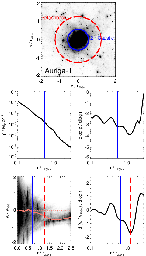
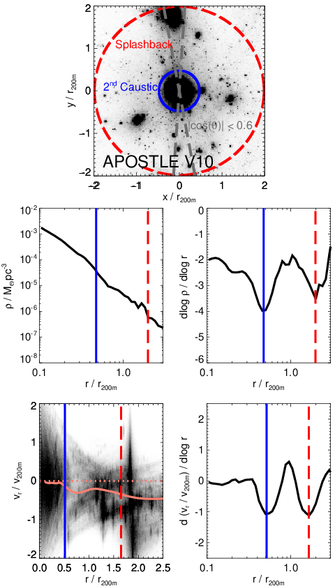
In Fig. 3 we show two example haloes. The left panels show the dark matter distribution of Auriga-1 (an isolated halo), and the right panels show APOSTLE V10 (a paired halo: in Fig. 3 the coordinate system is centred at $(x,y,z)=(61.948,24.230,48.305)$ Mpc in the V10 system, see Table A1 in Fattahi et al. 2016). The top panels show a 2D projection of the dark matter distribution, the middle panels the density profile and logarithmic slope profile, and the bottom panels the radial velocity profile and corresponding logarithmic slope profile. The dashed red lines indicate the splashback radius and the solid blue line the second caustic. For the paired haloes, caustics are identified by excluding position angles with $|\mathrm{cos}(\theta)|>0.6$. The second caustic is located at a smaller radius and is less pronounced than the splashback radius. We generally find that the second caustics are easier to identify in the individual halo density profiles, than in the stacked profiles (see e.g. Figs 1 and 2). This is likely because the feature is relatively weak and gets smeared out over a range of radii when the profiles are stacked together.

The second caustic can also be seen in the radial velocity profile. Here, we use the local minimum of $\mathrm{d}(v_{r})/\mathrm{d\,log}(r)$ to identify the caustics. The velocity and density caustics typically align on average, but there is some scatter (see Fig. 4). The radial velocity profile allows us to see more clearly what the second caustic is. The feature looks similar to the second caustic features shown in Adhikari et al. 2014, and we suggest that this feature relates to the edge of the material in the halo at the position where particles have completed at least two passages through pericentre. The splashback radius is located where material is outgoing for the first time, and particles have only completed one pericentric passage. The existence of two caustics, each defining different regions of the halo, begs the question: which should we use to define the edge of the halo? This question is particularly relevant for low mass accreting haloes, where the splashback and second caustic are well separated (Adhikari et al. 2014). Our Milky Way is located in the Local Group and neighbours a massive halo, so the definition of splashback radius is less clear (and indeed overlaps with the halo of M31). For this reason, we suggest that the most meaningful radius for the Milky Way is the second caustic. We will show in Section 3.2 that this definition is also applicable to the stellar material. Note, however, that although we have defined this interesting feature as the “second caustic”, this does not necessarily correspond to the classical definition of second caustic from spherical (or ellipsoidal) collapse models (as seen in Adhikari et al. 2014). In particular, the wide halo-to-halo scatter, and the apparent correlation with the stellar distribution (see following section), could point to a merger origin, i.e. from the apocentre of the last major merger. In addition, we caution that the second caustic, as we have defined it in this work, could have multiple origins that vary from halo-to-halo. The actual origin of this feature will require further investigation, ideally with particle evolution tracking.

In Fig. 4 we show the positions of the dark matter caustics for individual haloes in isolated (top panels) and paired (bottom panels) environments. The caustics are identified as minima in the $\mathrm{d\,log}(\rho)/\mathrm{d\,log}(r)$ and $\mathrm{d}(v_{r})/\mathrm{d\,log}(r)$ profiles. We consider the two most prominent (outer) caustics, and only consider features with $\mathrm{d\,log}(\rho)/\mathrm{d\,log}(r)<-2.5$ and $\mathrm{d}(v_{r})/\mathrm{d\,log}(r)<-0.25$, respectively. In addition, for every individual halo we visually inspect the profiles to ensure we are not confusing noise with a real caustic. The left panels show the position of the velocity caustics against the density caustics. The filled circles show the splashback radii and the open squares the second caustics. Note that for isolated haloes the splashback radius can be identified in almost all of the haloes; however, even with a restriction on position angle, this can be harder to detect in the paired haloes. Over all paired haloes (in ELVIS and APOSTLE) 21 percent have no detectable splashback radius in density or velocity. Moreover, the density and velocity caustics are not as closely aligned in the paired environments. On the other hand, the detection efficiency of the second caustic is very similar between isolated and paired haloes of similar mass (e.g. by comparing ELVIS Isolated and Paired haloes). There is no discernible second caustic in 16 percent of the haloes (over all haloes in ELVIS, APOSTLE and Auriga), and the non detections are typically more massive haloes with higher recent accretion rates (see below and Fig. 2). The detected second caustics range in radii between $0.3-0.8r_{\rm 200m}$ and have density slopes at these radii of $\sim-2.5$ to $-4.5$.

The symbols in Fig. 4 are coloured according to the recent mass accretion rate (see Eqn. 1). The majority of haloes have quite low recent mass accretion rates ($\Gamma<1$), as expected for Milky Way mass haloes. The middle panels of Fig. 4 show how the positions of the caustics relate to $\Gamma$. The caustics in the isolated haloes are typically at smaller radii for haloes with higher recent mass accretion rates (as shown in Diemer et al. 2017 over a wider mass range). However, this trend is not present in the paired environments, particularly for $\Gamma>1.5$. This is likely because the splashback radius and the second caustic run into each other at higher mass accretion rates, and are harder to distinguish. Furthermore, $\Gamma$ is poorly defined in paired environments where the outer profiles of the neighbouring haloes overlap. Finally, we show the location of the caustics as a function of halo mass in the right-hand panels. We see very little dependence between $R_{\rm Causitc}/r_{\rm 200m}$ and halo mass. Indeed, analytical models predict that mass accretion rate, rather than halo mass, is the more important physical quantity the determines the splashback radius (Adhikari et al. 2014, e.g.).

We now turn our attention to the stellar material in Milky Way-sized haloes. We analyse the APOSTLE and Auriga simulations which include baryonic material. In Fig. 5 we show the logarithmic slope of the stellar density profiles of the Auriga (left) and APOSTLE (right) haloes. We use the same bin sizes and smoothing technique as for the dark matter. As in Fig. 1, the median stacked profiles are shown, and the different colours show ten different intervals in position angle. The solid orange line shows the logarithmic slope of the median density profile for all haloes over all position angles. We indicate the minimum in the logarithmic slope for each position angle with dotted lines and we only consider minima with $\mathrm{d\,log}(\rho)/\mathrm{d\,log}(r)<-5$ (although typically the stellar caustics are much stronger than this, and range from $-15<\mathrm{d\,log}(\rho)/\mathrm{d\,log}(r)<-5$). The location of these minima are shown as a function of position angle in the adjacent plots (and colour coded accordingly). There is some variation of $R_{\rm Caustic}$ with position angle, but there is no obvious trend. It is notable that the profiles of the paired haloes (APOSTLE) and isolated haloes (Auriga) are similar, and the caustics are typically found at $0.6r_{\rm 200m}$. Interestingly, this is exactly the radius that we identified in Fig. 1 as the second caustic in the dark matter. Below, we focus on the profiles of individual haloes, and explicitly examine this apparent connection between the stars and dark matter.

We also show the logarithmic slope of the projected stellar density profiles in Fig. 6. Here we show the stacked profiles of all Auriga (left) and APOSTLE (right) haloes. This 2D measure is relevant for stellar halo density profiles of external Milky Way-mass galaxies for which only two spatial coordinates are known. The three different linestyles indicate three (random) projections, and the dotted red line shows the stacked 3D profile (repeated from Fig. 5 for comparison). A well-defined “edge” is also seen in the projected profiles. This occurs at slightly lower radii (in projection) relative to the 3D radius (by $\sim\!\!0.1r_{200m}$), and is a weaker feature than in the 3D profiles. However, the clear detection in 2D is encouraging for studies of external stellar haloes. Currently, surveys like Ghosts (Harmsen et al. 2017) and Dragonfly (Merritt et al. 2016) are only able to probe the stellar halo density out to $\sim\!\!50-80$ kpc. However, with deeper observations and future wide-field facilities such as the Nancy Grace Roman Space Telescope (Spergel et al. 2015), the radial range of interest, beyond 150 kpc should be accessible for nearby galaxies. Furthermore, the signal of the stellar edge could be enhanced by stacking the profiles of several galaxies.

In Fig. 7 we show the stellar distribution of two example haloes, Auriga-1 on the left and APOSTLE V10 on the right. The top panels show a 2D projection, the middle panels the stellar density and logarithmic slope profiles, and the bottom panels the radial velocity and associated logarithmic slope profiles. The solid orange line indicates the caustic in the stellar distribution. We typically identify only one clear outer caustic (cf. the dark matter where we commonly find two) at $\sim\!\!0.6r_{\rm 200m}$. However, there can be less prominent caustics at smaller radii, which are associated with apocentres of past accretion events (these can be seen in both dark matter and stars, see e.g. figs 3 and 7). Such a feature has already been seen in the Milky Way halo at $r\sim 20$ kpc, and is likely related to the apocentre of the Gaia-Sausage/Enceladus event (Deason et al. 2013; Deason et al. 2018). In this work we are interested in the caustic that defines the edge of the stellar material, and is hence associated with the furthest apocentre of stars bound to the Galaxy. The radial velocity profiles suggests that the location of this stellar caustic coincides with the edge of the material that has completed at least two pericentric passages, similarly to the second caustic in the dark matter (see below). We find no obvious difference between the isolated and paired haloes, which is unsurprising as the location of the stellar caustic ($0.6r_{\rm 200m}\sim r_{\rm 200c}\sim 220$ kpc) does not generally overlap with the neighbouring halo.

In Fig. 8 we examine the stellar caustics of individual haloes in more detail. We are able to identify a stellar caustic in over 90 percent of the haloes. Those cases where we cannot clearly identify a feature (in either density or velocity) are typically cases where there is very recent accretion and the outer density profiles are messy. Note we typically only consider stellar caustics with $\mathrm{d\,log}(\rho)/\mathrm{d\,log}(r)<-5$ or $\mathrm{d}\,(v_{r})/\mathrm{d\,log}(r)<-1.0$, which we choose to be distinct from the noise level. The left panel of Fig. 8 relates the positions of the velocity and density caustics of the stars. These caustics generally coincide but there is significant scatter. The points are colour coded according to the recent (total) mass accretion rate, $\Gamma(z=0.5)$ (see Eqn. 1). In the middle (density) and right-hand (velocity) panels we relate the stellar caustics to the dark matter caustics. Solid filled symbols are used for the splashback radii of the dark matter and open squares for the second caustic of the dark matter. As mentioned earlier, the stellar caustics are strongly related to the second caustic in the dark matter. Note the dashed line indicates the one-to-one relation; this is not a fit! This relation holds for $\sim(0.3-0.8)r_{\rm 200m}$, but seems to break down at larger radii. This discrepancy at large radii is likely for two reasons. Firstly, when $R^{\rm STAR}_{\rm Caustic}$ is large the stellar caustic can be closer to the splashback radii, or even somewhere between the second caustic and the splashback radius. Secondly, the stellar caustic is harder to define at very large distances ($0.8r_{\rm 200m}\sim 300$ kpc) where the density of stars is very low.

We leave a more thorough analysis of how the dynamics of the star particles relate to the dark matter to future work. However, it is worth discussing the possible origin of the correlation between the caustic in the stellar material and the second caustic in the dark matter. Firstly, we must consider that the stars and dark matter do not undergo the same evolution in the build-up of a halo. A significant amount of the dark matter is assembled by “smooth” accretion (Angulo & White 2010; Genel et al. 2010; Wang et al. 2011, e.g.). On the other hand, the stars are assembled from a “lumpier” accretion process, as the stars do not populate subhaloes below a certain mass threshold (Sawala et al. 2015, e.g.). Secondly, the stripping of stars from bound subhaloes proceeds differently to the stripping of the dark matter (Peñarrubia et al. 2008; Fattahi et al. 2018, e.g.): the (less bound) dark matter is stripped first, and the more centrally concentrated stars are almost always stripped close to pericentre, when almost all of the dark matter has already been peeled away.

We speculate that to lose stars to tidal forces subhaloes must typically pass through at least two pericentres, and thus the “edge” of the stellar material coincides with the second caustic in the dark matter. This may be especially true in relatively major mergers, which typically dominate the mass budget of the accreted stellar halo (see e.g. Purcell et al. 2007; Cooper et al. 2010; Deason et al. 2016; D’Souza & Bell 2018), when such passages lead to a loss of angular momentum and shrinking of the pericentre. Finally, we remark that the relation between the “edges” of stars and dark matter may vary at different mass scales. Here, we have focused on Milky Way-mass halos, but the non-linear stellar mass to dark matter mass relation (Behroozi et al. 2010; Moster et al. 2010; Read et al. 2017), and the varying smooth to lumpy mass accretion rate (Genel et al. 2010), will likely lead to different relations at higher and lower masses.

In Section 3.1 we discussed how the second caustic of the dark matter, which we now see coincides with the stellar caustic, may be the most relevant definition of the edge of the Milky Way. This means that the edge of our own Galaxy is, potentially, observable in the stellar distribution. Currently, the density profile of the stellar halo has only been mapped out to $\sim\!\!50-100$ kpc (Deason et al. 2011; Sesar et al. 2011; Deason et al. 2014a; Xue et al. 2015; Slater et al. 2016; Hernitschek et al. 2018, e.g.). Moreover, radial velocities of stars are only available, in any significant numbers, out to similar distances (Mauron et al. 2004; Deason et al. 2012; Bochanski et al. 2014; Cohen et al. 2017, e.g.). However, with upcoming wide-field photometric and spectroscopic facilities like the Rubin Observatory Legacy Survey of Space and Time (Ivezić et al. 2019, LSST,), the Roman Space Telescope (Spergel et al. 2015), the Mauna Kea Spectroscopic Explorer (Bauman et al. 2016, MSE,) and the Subaru Prime Focus Spectrograph (Takada et al. 2014, PFS,) on the horizon, exploring these extreme distances will be feasible in the near future.

Finally, it is worth discussing how the concept of galaxy edge is relevant to studies that require a definition of where the halo ends. For example, when using the escape velocity of local halo stars to estimate the total mass of the Galaxy, the definition of the radius of “escape” is an important element of the analysis. Indeed, Deason et al. 2019 used a radius of $2r_{\rm 200c}$ ($\sim\!\!1.25r_{\rm 200m}$), which is at the extreme end for the Auriga haloes. However, while this approach is conservative in that it does not allow for radii where stars can potentially escape, our results suggest that a smaller radius is likely more applicable. For example, the median stellar caustic radius of the Auriga simulations is $0.7r_{\rm 200m}$, which is approximately $1.2r_{\rm 200c}$. If this distance is used in the Deason et al. 2019 analysis to define the radius beyond which stars have escaped, then the total mass of the Milky Way is revised upwards by 20 percent. Interestingly, this is approximately the change that Grand et al. 2019a found was required to correct the mass estimates when the procedure is applied to the Auriga haloes. In particular, Grand et al. 2019a suggest that the mass estimates are underestimated because the local stars do not reach out to $2r_{\rm 200c}$. Here, we show that this is indeed the case. However, as a cautionary note, we should use the observed $R^{\rm STAR}_{\rm Caustic}$ rather than the median value of the Auriga haloes, which does not necessarily coincide with the true Milky Way value (see end of Section 3.3). Finally, we note that the term “escape velocity” is a misleading term when discussing the highest velocity halo stars. In reality, much faster stars would not “escape” as such, but rather they just do not exist in the stellar distribution.

In the previous subsections, we have focused on the distribution of dark matter and stars. Now we apply a similar analysis to the subhalo population. In this case, the number of discrete tracers is much lower than for the dark matter or star particles. For this reason, we concentrate only on the caustics defined in velocity space, where it is easier to identify features associated with caustics when there are low numbers of tracers. It is worth noting that there is no division into position angle sectors here (cf. the dark matter and stars), which makes the subhalo-based profiles sensitive to substructure. Thus, although this analysis is a valuable first step, we plan to apply more sophisticated techniques tailored towards highly discretely sampled distributions in future work.

We use the (dark matter only) ELVIS suite to study the general subhalo population, and APOSTLE and Auriga to analyse the “dwarf” population. Here we do not distinguish between isolated and paired environments and, in the paired cases, only consider subhaloes with $|\mathrm{cos}(\theta)|<0.6$ to identify caustics. We define subhaloes as all bound substructures with $M^{\rm DM}_{\rm Sub}>10^{7.3}\mathrm{M}_{\odot}$. This is the convergence limit for subhaloes found by Garrison-Kimmel et al. 2014. In APOSTLE and Auriga, subhaloes with at least one star particle are identified as luminous dwarfs. This approximately corresponds to subhaloes with $M^{\rm Star}_{\rm Sub}>10^{5}\mathrm{M}_{\odot}$.

For each individual halo we use the logarithmic slope of the radial velocity profile to define the caustics in the subhalo population. Note that for the dwarf galaxies, where the numbers of objects are typically low (O(100) per halo), we change the binning in logarithmic radius to have 25 equally spaced bins in the range $\mathrm{log}(r/r_{\rm 200m})\in[-1.0,0.5]$ and use the same smoothing kernel as in the previous subsections. Due to the small numbers we only identify the most prominent caustic and do not attempt to find two distinct caustics.

The resulting caustics are shown in Fig. 9 as a function of the (two) dark matter caustics (computed in Section 3.1). Caustics can be identified for the majority of subhalo populations, but in several cases (30 percent) a caustic could not be identified in the dwarf population, mainly as a result of small numbers. The filled gray circles in Fig. 9 indicate the splashback radii in the dark matter and the filled red squares the second caustic in the dark matter. Interestingly, we find that the caustic in the subhalo population corresponds to the splashback radius (left panel), while the caustic in the luminous dwarfs’ population coincides with the second caustic in the dark matter (right panel). This is perhaps unsurprising as the subhalo population traces the dark matter, while the luminous dwarfs are more closely related to the accretion of the more massive subhaloes, and hence the stellar halo.

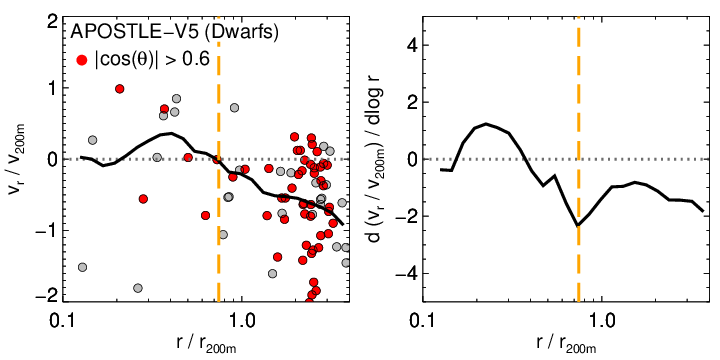
We show two examples for the dwarf galaxy population in Auriga-16 (top panel) and APOSTLE-V5 (bottom panel; centred centred on $(x,y,z)=(42.867,88.474,93.675)$ Mpc) in Fig. 10. The caustics are not as clearly defined as in the dark matter or stars, but, importantly, there are already observations of luminous dwarf tracers out to large distances in the Local Group, so this analysis is observationally motivated. In Fig.  11 we perform the same analysis on the observed dwarfs. Here, we use the latest compilation of dwarfs from McConnachie 2012, and show physical radius and velocity (rather than in units of $r_{\rm 200m}$ and $v_{\rm 200m}$). The distances and and radial velocities are converted to Galactocentric coordinates, assuming a circular velocity of $v_{c}(r_{0})=235$ km s^-1 at the position of the Sun ($r_{0}=8.1$ kpc), and a peculiar solar motion of ($U_{\odot},V_{\odot},W_{\odot})=(11.1,12.24,7.25)$ km s^-1 (Schönrich et al. 2010). We use 22 radial bins equally spaced in $\mathrm{log}(r)$ between $1.0$ and $3.3$. As we did previously, the logarithmic slope profile is computed using the fourth-order Savitzky–Golay smoothing algorithm over the 15 nearest bins (Savitzky & Golay 1964). We indicate in the figure dwarfs which are close in angle to the line joining the Milky Way and M31 (i.e $|\mathrm{cos}(\theta)>0.6|$). In practice, we find little difference if we include or exclude these dwarfs.

We identify a minimum in the observed population of dwarfs at $\sim\!\!290$ kpc. Using a bootstrap method to estimate the uncertainty, we find $R_{\rm edge}=292\pm 61$ kpc. If we assume the Milky Way halo mass recently measured by Callingham et al. 2019 and a typical halo concentration ($\sim\!\!10$ for Milky Way-mass haloes; Neto et al. 2007; Ludlow et al. 2014; Klypin et al. 2016), this radius corresponds to $0.8r_{\rm 200m}$ (or $1.3r_{\rm 200c}$). Interestingly, this radius (292 kpc) lies at exactly the “virial radius” defined by the fitting formulae in Bryan & Norman 1998. Moreover, this also coincides with the radius where the Hi content of Local Group satellites sharply drops (around 270 kpc, Grcevich & Putman 2009). Given the rather large uncertainty in the measurement, these could simply be coincidences, however, it is worth noting that we are probing an interesting radial regime of the Galactic halo.

We can also use this measured radius to independently estimate the mass of the Milky Way using the escape velocity analysis described by Deason et al. 2019. As mentioned in Section 3.2, this technique depends on the definition of the “outer boundary” of the halo stars. If we use a boundary of 290 kpc, rather than a fixed fraction of $r_{\rm 200c}$ like Deason et al. 2019, we find a mass of $M_{\rm 200c}\sim 1.1\times 10^{12}M_{\odot}$. Although there is considerable uncertainty in this definition of halo edge, it is reassuring that this mass is in excellent agreement with the recent measurements by Callingham et al. 2019 and Cautun et al. 2020.

While we suggest that the edge of the Milky Way halo lies at 290 kpc, this remains a tentative result for two important reasons. Firstly, the value is strongly dependent on Leo I (located at 250 kpc): there is a significant gap between the most distant satellite of the Milky Way and the nearest dwarfs in the Local Group. Secondly, and perhaps most importantly, our census of local dwarfs is far from complete and we have made no attempt to correct for selection effects or observational biases. Indeed, as recently predicted by Fattahi et al. 2020, there are troves of local group dwarfs waiting to be discovered by future wide-field imaging surveys.

References

- Adhikari et al. (2014) Adhikari S., Dalal N., Chamberlain R. T., 2014, J. Cosmology Astropart. Phys., 2014, 019
- Angulo & White (2010) Angulo R. E., White S. D. M., 2010, MNRAS, 401, 1796
- Ascasibar et al. (2007) Ascasibar Y., Hoffman Y., Gottlöber S., 2007, MNRAS, 376, 393
- Bahé et al. (2013) Bahé Y. M., McCarthy I. G., Balogh M. L., Font A. S., 2013, MNRAS, 430, 3017
- Balogh et al. (2000) Balogh M. L., Navarro J. F., Morris S. L., 2000, ApJ, 540, 113
- Bauman et al. (2016) Bauman S. E., et al., 2016, MSE observatory: a revised and optimized astronomical facility. SPIE, p. 990605, doi:10.1117/12.2234311
- Baxter et al. (2017) Baxter E., et al., 2017, ApJ, 841, 18
- Behroozi et al. (2010) Behroozi P. S., Conroy C., Wechsler R. H., 2010, ApJ, 717, 379
- Behroozi et al. (2013a) Behroozi P. S., Wechsler R. H., Wu H.-Y., 2013a, ApJ, 762, 109
- Behroozi et al. (2013b) Behroozi P. S., Wechsler R. H., Wu H.-Y., Busha M. T., Klypin A. A., Primack J. R., 2013b, ApJ, 763, 18
- Belokurov et al. (2020) Belokurov V., Sanders J. L., Fattahi A., Smith M. C., Deason A. J., Evans N. W., Grand R. J. J., 2020, MNRAS, 494, 3880
- Berlind & Weinberg (2002) Berlind A. A., Weinberg D. H., 2002, ApJ, 575, 587
- Bertschinger (1985) Bertschinger E., 1985, ApJS, 58, 39
- Binney & Tremaine (2008) Binney J., Tremaine S., 2008, Galactic Dynamics: Second Edition. Princeton University Press, Princeton, NJ USA
- Bochanski et al. (2014) Bochanski J. J., Willman B., Caldwell N., Sand erson R., West A. A., Strader J., Brown W., 2014, ApJ, 790, L5
- Boylan-Kolchin et al. (2011) Boylan-Kolchin M., Bullock J. S., Kaplinghat M., 2011, MNRAS, 415, L40
- Bryan & Norman (1998) Bryan G. L., Norman M. L., 1998, ApJ, 495, 80
- Bullock et al. (2001) Bullock J. S., Kolatt T. S., Sigad Y., Somerville R. S., Kravtsov A. V., Klypin A. A., Primack J. R., Dekel A., 2001, MNRAS, 321, 559
- Busch & White (2017) Busch P., White S. D. M., 2017, MNRAS, 470, 4767
- Callingham et al. (2019) Callingham T. M., et al., 2019, MNRAS, 484, 5453
- Campbell et al. (2017) Campbell D. J. R., et al., 2017, MNRAS, 469, 2335
- Cautun et al. (2020) Cautun M., et al., 2020, MNRAS, 494, 4291
- Chang et al. (2018) Chang C., et al., 2018, ApJ, 864, 83
- Cohen et al. (2017) Cohen J. G., Sesar B., Bahnolzer S., He K., Kulkarni S. R., Prince T. A., Bellm E., Laher R. R., 2017, ApJ, 849, 150
- Cole & Lacey (1996) Cole S., Lacey C., 1996, MNRAS, 281, 716
- Contigiani et al. (2019) Contigiani O., Hoekstra H., Bahé Y. M., 2019, MNRAS, 485, 408
- Cooper et al. (2010) Cooper A. P., et al., 2010, MNRAS, 406, 744
- Crain et al. (2015) Crain R. A., et al., 2015, MNRAS, 450, 1937
- D’Souza & Bell (2018) D’Souza R., Bell E. F., 2018, MNRAS, 474, 5300
- Davis et al. (1985) Davis M., Efstathiou G., Frenk C. S., White S. D. M., 1985, ApJ, 292, 371
- Deason et al. (2011) Deason A. J., Belokurov V., Evans N. W., 2011, MNRAS, 416, 2903
- Deason et al. (2012) Deason A. J., et al., 2012, MNRAS, 425, 2840
- Deason et al. (2013) Deason A. J., Belokurov V., Evans N. W., Johnston K. V., 2013, ApJ, 763, 113
- Deason et al. (2014a) Deason A. J., Belokurov V., Koposov S. E., Rockosi C. M., 2014a, ApJ, 787, 30
- Deason et al. (2014b) Deason A., Wetzel A., Garrison-Kimmel S., 2014b, ApJ, 794, 115
- Deason et al. (2016) Deason A. J., Mao Y.-Y., Wechsler R. H., 2016, ApJ, 821, 5
- Deason et al. (2017) Deason A. J., Belokurov V., Koposov S. E., Gómez F. A., Grand R. J., Marinacci F., Pakmor R., 2017, MNRAS, 470, 1259
- Deason et al. (2018) Deason A. J., Belokurov V., Koposov S. E., Lancaster L., 2018, ApJ, 862, L1
- Deason et al. (2019) Deason A. J., Fattahi A., Belokurov V., Evans N. W., Grand R. J. J., Marinacci F., Pakmor R., 2019, MNRAS, 485, 3514
- Diemand & Kuhlen (2008) Diemand J., Kuhlen M., 2008, ApJ, 680, L25
- Diemand et al. (2007) Diemand J., Kuhlen M., Madau P., 2007, ApJ, 667, 859
- Diemer & Kravtsov (2014) Diemer B., Kravtsov A. V., 2014, ApJ, 789, 1
- Diemer et al. (2013) Diemer B., More S., Kravtsov A. V., 2013, ApJ, 766, 25
- Diemer et al. (2017) Diemer B., Mansfield P., Kravtsov A. V., More S., 2017, ApJ, 843, 140
- Eke et al. (1998) Eke V. R., Navarro J. F., Frenk C. S., 1998, ApJ, 503, 569
- Fattahi et al. (2016) Fattahi A., et al., 2016, MNRAS, 457, 844
- Fattahi et al. (2018) Fattahi A., Navarro J. F., Frenk C. S., Oman K. A., Sawala T., Schaller M., 2018, MNRAS, 476, 3816
- Fattahi et al. (2019) Fattahi A., et al., 2019, MNRAS, 484, 4471
- Fattahi et al. (2020) Fattahi A., Navarro J. F., Frenk C. S., 2020, MNRAS, 493, 2596
- Fillmore & Goldreich (1984) Fillmore J. A., Goldreich P., 1984, ApJ, 281, 1
- Frenk et al. (1988) Frenk C. S., White S. D. M., Davis M., Efstathiou G., 1988, ApJ, 327, 507
- Garrison-Kimmel et al. (2014) Garrison-Kimmel S., Boylan-Kolchin M., Bullock J. S., Lee K., 2014, MNRAS, 438, 2578
- Garrison-Kimmel et al. (2017) Garrison-Kimmel S., Bullock J. S., Boylan-Kolchin M., Bardwell E., 2017, MNRAS, 464, 3108
- Genel et al. (2010) Genel S., Bouché N., Naab T., Sternberg A., Genzel R., 2010, ApJ, 719, 229
- Genina et al. (2018) Genina A., et al., 2018, MNRAS, 474, 1398
- Genina et al. (2019) Genina A., et al., 2019, arXiv e-prints, p. arXiv:1911.09124
- Gill et al. (2005) Gill S. P. D., Knebe A., Gibson B. K., 2005, MNRAS, 356, 1327
- Grand et al. (2016) Grand R. J. J., et al., 2016, MNRAS, 460, L94
- Grand et al. (2017) Grand R. J. J., et al., 2017, MNRAS, 467, 179
- Grand et al. (2018) Grand R. J. J., et al., 2018, MNRAS, 474, 3629
- Grand et al. (2019a) Grand R. J. J., Deason A. J., White S. D. M., Simpson C. M., Gómez F. A., Marinacci F., Pakmor R., 2019a, MNRAS, 487, L72
- Grand et al. (2019b) Grand R. J. J., et al., 2019b, MNRAS, 490, 4786
- Grcevich & Putman (2009) Grcevich J., Putman M. E., 2009, ApJ, 696, 385
- Gunn & Gott (1972) Gunn J. E., Gott J. Richard I., 1972, ApJ, 176, 1
- Harmsen et al. (2017) Harmsen B., Monachesi A., Bell E. F., de Jong R. S., Bailin J., Radburn-Smith D. J., Holwerda B. W., 2017, MNRAS, 466, 1491
- Hayashi & White (2008) Hayashi E., White S. D. M., 2008, MNRAS, 388, 2
- Hernitschek et al. (2018) Hernitschek N., et al., 2018, ApJ, 859, 31
- Ivezić et al. (2019) Ivezić Ž., et al., 2019, ApJ, 873, 111
- Jenkins (2013) Jenkins A., 2013, MNRAS, 434, 2094
- Klypin et al. (2016) Klypin A., Yepes G., Gottlöber S., Prada F., Heß S., 2016, MNRAS, 457, 4340
- Knebe et al. (2011) Knebe A., et al., 2011, MNRAS, 415, 2293
- Komatsu et al. (2011) Komatsu E., et al., 2011, ApJS, 192, 18
- Kravtsov (2013) Kravtsov A. V., 2013, ApJ, 764, L31
- Kravtsov et al. (2004) Kravtsov A. V., Berlind A. A., Wechsler R. H., Klypin A. A., Gottlöber S., Allgood B. o., Primack J. R., 2004, ApJ, 609, 35
- Lahav et al. (1991) Lahav O., Lilje P. B., Primack J. R., Rees M. J., 1991, MNRAS, 251, 128
- Larson et al. (2011) Larson D., et al., 2011, ApJS, 192, 16
- Leonard & Tremaine (1990) Leonard P. J. T., Tremaine S., 1990, ApJ, 353, 486
- Lovell et al. (2017) Lovell M. R., et al., 2017, MNRAS, 468, 4285
- Ludlow et al. (2009) Ludlow A. D., Navarro J. F., Springel V., Jenkins A., Frenk C. S., Helmi A., 2009, ApJ, 692, 931
- Ludlow et al. (2010) Ludlow A. D., Navarro J. F., Springel V., Vogelsberger M., Wang J., White S. D. M., Jenkins A., Frenk C. S., 2010, MNRAS, 406, 137
- Ludlow et al. (2014) Ludlow A. D., Navarro J. F., Angulo R. E., Boylan-Kolchin M., Springel V., Frenk C., White S. D. M., 2014, MNRAS, 441, 378
- Mamon et al. (2004) Mamon G. A., Sanchis T., Salvador-Solé E., Solanes J. M., 2004, A&A, 414, 445
- Mansfield et al. (2017) Mansfield P., Kravtsov A. V., Diemer B., 2017, ApJ, 841, 34
- Marinacci et al. (2017) Marinacci F., Grand R. J. J., Pakmor R., Springel V., Gómez F. A., Frenk C. S., White S. D. M., 2017, MNRAS, 466, 3859
- Mauron et al. (2004) Mauron N., Azzopardi M., Gigoyan K., Kendall T. R., 2004, A&A, 418, 77
- McConnachie (2012) McConnachie A. W., 2012, AJ, 144, 4
- Merritt et al. (2016) Merritt A., van Dokkum P., Abraham R., Zhang J., 2016, ApJ, 830, 62
- Monachesi et al. (2016) Monachesi A., Gómez F. A., Grand R. J. J., Kauffmann G., Marinacci F., Pakmor R., Springel V., Frenk C. S., 2016, MNRAS, 459, L46
- Monachesi et al. (2019) Monachesi A., et al., 2019, MNRAS, 485, 2589
- Moore et al. (1999a) Moore B., Quinn T., Governato F., Stadel J., Lake G., 1999a, MNRAS, 310, 1147
- Moore et al. (1999b) Moore B., Ghigna S., Governato F., Lake G., Quinn T., Stadel J., Tozzi P., 1999b, ApJ, 524, L19
- More et al. (2015) More S., Diemer B., Kravtsov A. V., 2015, ApJ, 810, 36
- More et al. (2016) More S., et al., 2016, ApJ, 825, 39
- Moster et al. (2010) Moster B. P., Somerville R. S., Maulbetsch C., van den Bosch F. C., Macciò A. V., Naab T., Oser L., 2010, ApJ, 710, 903
- Murata et al. (2020) Murata R., Sunayama T., Oguri M., More S., Nishizawa A. J., Nishimichi T., Osato K., 2020, arXiv e-prints, p. arXiv:2001.01160
- Navarro et al. (1996) Navarro J. F., Frenk C. S., White S. D. M., 1996, ApJ, 462, 563
- Navarro et al. (1997) Navarro J. F., Frenk C. S., White S. D. M., 1997, ApJ, 490, 493
- Neto et al. (2007) Neto A. F., et al., 2007, MNRAS, 381, 1450
- Pawlowski et al. (2017) Pawlowski M. S., Ibata R. A., Bullock J. S., 2017, ApJ, 850, 132
- Peñarrubia et al. (2008) Peñarrubia J., Navarro J. F., McConnachie A. W., 2008, ApJ, 673, 226
- Planck Collaboration et al. (2014) Planck Collaboration et al., 2014, A&A, 571, A16
- Prada et al. (2006) Prada F., Klypin A. A., Simonneau E., Betancort-Rijo J., Patiri S., Gottlöber S., Sanchez-Conde M. A., 2006, ApJ, 645, 1001
- Purcell et al. (2007) Purcell C. W., Bullock J. S., Zentner A. R., 2007, ApJ, 666, 20
- Read et al. (2017) Read J. I., Iorio G., Agertz O., Fraternali F., 2017, MNRAS, 467, 2019
- Sales et al. (2007) Sales L. V., Navarro J. F., Abadi M. G., Steinmetz M., 2007, MNRAS, 379, 1475
- Savitzky & Golay (1964) Savitzky A., Golay M. J. E., 1964, Analytical Chemistry, 36, 1627
- Sawala et al. (2015) Sawala T., et al., 2015, MNRAS, 448, 2941
- Sawala et al. (2016) Sawala T., et al., 2016, MNRAS, 457, 1931
- Sawala et al. (2017) Sawala T., Pihajoki P., Johansson P. H., Frenk C. S., Navarro J. F., Oman K. A., White S. D. M., 2017, MNRAS, 467, 4383
- Schaye et al. (2015) Schaye J., et al., 2015, MNRAS, 446, 521
- Schönrich et al. (2010) Schönrich R., Binney J., Dehnen W., 2010, MNRAS, 403, 1829
- Sesar et al. (2011) Sesar B., Jurić M., Ivezić Ž., 2011, ApJ, 731, 4
- Shin et al. (2019) Shin T., et al., 2019, MNRAS, 487, 2900
- Shull (2014) Shull J. M., 2014, ApJ, 784, 142
- Simpson et al. (2018) Simpson C. M., Grand R. J. J., Gómez F. A., Marinacci F., Pakmor R., Springel V., Campbell D. J. R., Frenk C. S., 2018, MNRAS, 478, 548
- Slater et al. (2016) Slater C. T., Nidever D. L., Munn J. A., Bell E. F., Majewski S. R., 2016, ApJ, 832, 206
- Spergel et al. (2015) Spergel D., et al., 2015, arXiv e-prints, p. arXiv:1503.03757
- Springel (2005) Springel V., 2005, MNRAS, 364, 1105
- Springel et al. (2001) Springel V., White S. D. M., Tormen G., Kauffmann G., 2001, MNRAS, 328, 726
- Springel et al. (2008) Springel V., et al., 2008, MNRAS, 391, 1685
- Stadel et al. (2009) Stadel J., Potter D., Moore B., Diemand J., Madau P., Zemp M., Kuhlen M., Quilis V., 2009, MNRAS, 398, L21
- Starkenburg et al. (2017) Starkenburg E., Oman K. A., Navarro J. F., Crain R. A., Fattahi A., Frenk C. S., Sawala T., Schaye J., 2017, MNRAS, 465, 2212
- Takada et al. (2014) Takada M., et al., 2014, PASJ, 66, R1
- Teyssier et al. (2012) Teyssier M., Johnston K. V., Kuhlen M., 2012, MNRAS, 426, 1808
- Wang et al. (2011) Wang J., et al., 2011, MNRAS, 413, 1373
- Wechsler & Tinker (2018) Wechsler R. H., Tinker J. L., 2018, ARA&A, 56, 435
- Wechsler et al. (2002) Wechsler R. H., Bullock J. S., Primack J. R., Kravtsov A. V., Dekel A., 2002, ApJ, 568, 52
- Wetzel et al. (2014) Wetzel A. R., Tinker J. L., Conroy C., van den Bosch F. C., 2014, MNRAS, 439, 2687
- Wetzel et al. (2015) Wetzel A. R., Deason A. J., Garrison-Kimmel S., 2015, ApJ, 807, 49
- Xhakaj et al. (2019) Xhakaj E., Diemer B., Leauthaud A., Wasserman A., Huang S., Luo Y., Adhikari S., Singh S., 2019, arXiv e-prints, p. arXiv:1911.09295
- Xue et al. (2015) Xue X.-X., Rix H.-W., Ma Z., Morrison H., Bovy J., Sesar B., Janesh W., 2015, ApJ, 809, 144
- Zavala et al. (2008) Zavala J., Okamoto T., Frenk C. S., 2008, MNRAS, 387, 364
- Zürcher & More (2019) Zürcher D., More S., 2019, ApJ, 874, 184