Massive MIMO Channel Measurements and Achievable Rates in a Residential Area

The transmitter is based on an Ettus USRP B210 [6]. Its fpga (fpga) was programmed to generate ofdm (ofdm) symbols of $B=18\,\mathrm{MHz}$ effective bandwidth. An ofdm sample rate of $R_{s}=\frac{1}{T_{s}}=20\,\mathrm{MS/s}$ and a number of $N_{\text{sub}}=1024$ subcarriers are used. The subcarrier spacing is about $\Delta f_{\text{sub}}=\frac{R_{s}}{N_{\text{sub}}}\approx 20\,\mathrm{kHz}$. At either band edge, 49-50 subcarriers were set to zero to relax the requirements for analog filtering; also, the dc (dc) subcarrier was set to zero for carrier leakage reduction; thus, in total 924 subcarriers are effectively used, as depicted in Fig. 1. The carrier frequency was set to the unlicensed ham radio frequency $1.27\,\mathrm{GHz}$ so that a rather large transmit pep (pep) of $18\,\mathrm{W}$ ($P_{\text{TX}}=42\,\mathrm{dBm}$) in combination with a dipole antenna could be used. In this frequency range a pep of up to $750\,\mathrm{W}$ is allowed for licensed ham radio. The transmitter dipole antenna has a gain of about $G_{\text{TX}}=9\,\mathrm{dBi}$ and is vertically polarized, yielding an eirp (eirp) of about $51\,\mathrm{dBm}$.

Fig. 3 shows the link budget for a los channel. $G_{RX}$ is the rx (rx) antenna gain. The total measurement time was 8 hours, where the compact hand-wagon was manually pushed around in a residential area of size about $600\,\mathrm{m}\times 800\,\mathrm{m}$ (Fig. 2).

The receiver uses a 64-element antenna array with dual polarized patch antennas, while only the vertical polarization was used. The 64 full rf (rf) chains are implemented in a multi-board/daughter-board configuration to filter, amplify and downconvert (i.e., frequency shift) the respective antenna signals. The 64 antenna signals of $18\,\mathrm{MHz}$ bandwidth, all centered around the carrier frequency of $1.27\,\mathrm{GHz}$, are shifted to different intermediate frequencies by means of separately programmable downconverters so that the individual spectra do not overlap in a spectral band from $10\,\mathrm{MHz}$ to $2\,\mathrm{GHz}$. This composite “frequency division multiple antenna”-signal is then analog-to-digital converted and stored on a ssd (ssd) drive by a digital oscilloscope Teledyne LeCroy WavePro 604HD, allowing to measure spatial snapshots of 64 antennas times 924 subcarriers complex csi (csi) samples at a rate of ~11 measurements points per second (comp. [8] for more details).

All 64 antenna signals are perfectly time synchronized in the digital domain by jointly digitizing the composite “frequency division multiple antenna”-signal using the single adc (adc) of the digital scope (in fact, four adcs of the scope were used which, however, are perfectly synchronized). The repeated two pilots symbols are used for the frame detection, channel estimation and for cfo estimation by employing

To obtain a measurement set-up which is stable over several hours, all csi phases are calibrated to a reference transmitter which was at a fixed position only a few meters away from the antenna array. The (narrowband) reference transmitter was set to a carrier frequency of $1.257\,\mathrm{GHz}$ with a spectral bandwidth of $1.5\,\mathrm{MHz}$. This way, any phase jitter/phase flips etc. of the rf chains that may occur due to the individual pll (pll) control loops are implicitly accounted for. Also, to account for different gains of the rf chains, the power of the individual signals is further calibrated by estimating the snr (snr) per rf-chain, and aligning the noise floor across all antenna signals by respective amplitude scaling. To further reduce the noise, i.e., to improve the snr, the time-domain channel impulse response was computed from the frequency domain channel estimates csi, and cut off so that multipath delays up to $0.82\,\mathrm{ms}$ corresponding to a maximal path difference of $1.92\,\mathrm{km}$ were accounted for (i.e., 128 samples at $T_{s}=\frac{1}{20}\mu s$). The rx antenna array was located at position $\left(x,y\right)=\left(0\mathrm{m},0\mathrm{m}\right)$ on a roof-top height of $40\,\mathrm{m}$ above ground and is marked in the figures with a red cross (“X”). The rx antenna array was facing toward the South-East.

Fig. 7 plots the mean snr computed across all 64 rx antennas. As expected, the area in the North has to have a smaller snr due to the limited half power beam width of $69.1\,\mathrm{{{}^{\circ}}}$ of the receiver array’s patch antennas.

As one sanity check for the measured data, Fig. 8 illustrates the distribution of the signal power if mrt precoding is applied to a position at $(110\mathrm{m},-120\mathrm{m})$, resulting in a quite plausible beam/focus area around the desired “target” user point in comparison to the “mean-SNR” shown in Fig. 7 .

Next, we outline the details of the clustering algorithm for the two precoding techniques mrt and po (po), respectively. Algorithm 1 describes a $k$-means clustering with an mrt precoding weight function, and Algorithm 2 describes the version using a po weight function.

Fig. 11 shows exemplary the clustering results for the $k$-means mrt-based clustering algorithm for $k=40$ clusters after 30 iterations. The positions of the specific channel measurement are colored according to their respective cluster. Fig. 12 shows the clustering results for the $k$-means po clustering algorithm for the respective value of $k$, number of iterations and the same randomly picked initial cluster centers. Obviously, channel measurements which are locally close to each other are grouped into the same cluster. The result shows an expected behavior from other channel models. It is yet another sanity check for the measurements. The regions with low snr result in higher diversity of clusters (with, yet, only small contribution to sum rate) and the regions with higher snrs show more separated clusters. The reason for this effect is that two channels “decorrelate” with increasing noise power.

To evaluate the results of the clustering algorithms, the sum-rate was calculated while assuming an interference-limited channel. To account for the noise, the sir (sir) is clipped to a sir of $30\,\mathrm{dB}$.

The $\text{\text{SIR}}_{u}$ for user $u$ that belongs to cluster $k$ is calculated according to

The cluster $\text{\text{SIR}}_{k}$ is calculated by the median of the $\text{\text{SIR}}_{u}$ of all users within this cluster $k$. The interference is calculated by the sum of the energy for user $u$ from all clusters $\hat{k}$ without cluster $k$.

The sum-rate $R_{\text{sum}}$ is calculated by the sum of the rate of its respective cluster $\text{\text{SIR}}_{k}$.

Fig. 13 shows the mean of the sum-rate after 1000 random initializations of the $k$-means clustering algorithm. The increasing number of clusters results in a small increase of the sum-rate. After $k\geq 20$ clusters, mrt-precoding begins to significantly outperform po-precoding. Note that mrt-precoding should be better than po-precoding for all $k$, indicating that the number of random initializations for computing the median could still be increased.

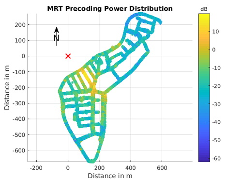
However, the result also indicates that the lower complexity po-precoding only incurs a small loss with respect to mrt-precoding for lower number $k$ of clusters. For a small number of clusters, e.g., $k=5$, both clustering algorithms converge to nearly the same clusters. For small $k$, e.g., $k<20$, the po-algorithm approaches the mrt-algorithm performance very closely. Note that, the po-algorithm considers only the phase and is, thus, of much lower complexity (akin beam-forming). The beam-forming characteristics can clearly be observed in Fig. 10 and Fig. 9. If the number of clusters $k$ increases to, e.g., $k=40$, the clusters have to be separated not only in the angular direction but also in the radial distance, such that several clusters are “behind” each other in radial direction; in this case, the mrt-algorithm outperforms the po-based cluster algorithm. Fig. 11 and Fig. 12 show the different clustering results for the exact same initial cluster centers for $k=40$.

References

- [1] E. Björnson, J. Hoydis and L. Sanguinetti, Massive MIMO Networks: Spectral, Energy, and Hardware Efficiency. Now Publisher, Feb. 2017.
- [2] E. G. Larsson, O. Edfors, F. Tufvesson, and T. L. Marzetta, “Massive MIMO for next generation wireless systems,” IEEE Communications Magazine, 2014.
- [3] J. Hoydis, S. ten Brink, and M. Debbah, “Massive MIMO in the UL/DL of Cellular Networks: How Many Antennas Do We Need?” IEEE Journal on Selected Areas in Communications, 2013.
- [4] S. Jaeckel, L. Raschkowski, K. Borner, and L. Thiele, “QuaDRiGa: A 3-D multi-cell channel model with time evolution for enabling virtual field trials,” IEEE Trans. Antennas Propag., pp. 1–6, Oct. 2014.
- [5] R. S. Ganesan and W. Zirwas and B. Panzner and K. I. Pedersen and K. Valkealahti, “Integrating 3D Channel Model and Grid of Beams for 5G mMIMO System Level Simulations,” in Vehicular Technology Conference, Sept. 2016, pp. 1–6.
- [6] USRP User Manual, Ettus Research. [Online]. Available: https://www.ettus.com/
- [7] T. Takasu and A. Yasuda, “Development of the low-cost RTK-GPS receiver with an open source program package RTKLIB,” International Symposium on GPS/GNSS, International Convention Center Jeju, Korea, November 4-6, Tech. Rep., 2009.
- [8] M. Arnold and J. Hoydis and S. ten Brink, “Novel Massive MIMO Channel Sounding Data Applied to Deep Learning-based Indoor Positioning,” International Conference on Systems, Communications and Coding (SCC), pp. 1–6, Feb. 2019.
- [9] M. Arnold, J. Pfeiffer, and S. ten Brink, “Area Rate Evaluation based on Spatial Clustering of massive MIMO Channel Measurements,” in WSA 2018; 22nd International ITG Workshop on Smart Antennas, March 2018, pp. 1–6.