Minimizing Localized Ratio Cut Objectives in HypergraphsConference: ; ;

Let $G=(V,E)$ be an undirected graph and $w_{ij}\geq 0$ be the weight for edge $(i,j)\in E$. The degree of a node $v$ is $d_{v}=\sum_{u\in N_{v}}w_{uv}$, where $N_{v}$ is the set of nodes sharing an edge with $v$. A common graph clustering objective is conductance, defined for $S\subseteq V$ by

where $\textbf{vol}(S)=\sum_{v\in S}d_{v}$ is the volume of nodes in $S$, and $\textbf{cut}(S)=\sum_{i\in S,j\in\bar{S}}w_{ij}$, which equals $\textbf{cut}(\bar{S})$ by definition. Here, $\bar{S}=V\backslash S$ is the complement set of $S$. A related objective, which differs by at most a factor of two from conductance, is normalized cut (shimalik-ncut):

Conductance and normalized cut are both NP-hard to minimize (wagner1993between). However, localized variants can be minimized in polynomial time with repeated max. $s$-$t$ flow computations (Andersen:2008:AIG:1347082.1347154; LangRao2004; Orecchia:2014:FAL:2634074.2634168; veldt16simple; Veldt2019flow). For example, given nodes $R\subseteq V$ with $\textbf{vol}(R)\leq\textbf{vol}(\bar{R})$, the following objective can be minimized in polynomial time (LangRao2004):

In other words, given a region defined by a reference set $R$, one can find the minimum conductance subset of $R$ in polynomial time, even though minimizing conductance over an entire graph is NP-hard. A more general local conductance objective is

Objective (4) is minimized over all sets of nodes for which the denominator is positive (to avoid trivial outputs). The denominator rewards sets $S$ that overlap with $R$. The locality parameter $\varepsilon$ controls the penalty for including nodes outside $R$. As $\varepsilon\rightarrow\infty$, minimizing Eq. (4) over sets producing a positive denominator becomes equivalent to Eq. (3). Andersen and Lang (Andersen:2008:AIG:1347082.1347154) showed how to minimize this objective for $\varepsilon=\textbf{vol}(R)/\textbf{vol}(\bar{R})$, and faster algorithms were later developed for $\varepsilon\gg\textbf{vol}(R)/\textbf{vol}(\bar{R})$ (Orecchia:2014:FAL:2634074.2634168; veldt16simple). These algorithms repeatedly solve maximum flow problems on an auxiliary graph.

Minimizing objective (4) can also provide cluster quality guarantees in terms of standard conductance (Eq. (1)). For example, the optimal set for (4) with $\varepsilon=\textbf{vol}(R)/\textbf{vol}(\bar{R})$ has conductance within a small factor of the conductance of any set with a certain amount of overlap with $R$ (Andersen:2008:AIG:1347082.1347154), and there are related results for other values of $\varepsilon$ and objectives (Veldt2019flow; veldt16simple; Orecchia:2014:FAL:2634074.2634168). These are often called cut improvement guarantees, since the ratio cut score of the output set improves upon the score of the input $R$. See the work of Fountoulakis et al. (fountoulakis2020flowbased) for a detailed survey on flow-based methods for solving objective (4).

We now consider a hypergraph $\mathcal{H}=(V,E)$, where each edge $e\in E$ is a subset of $V$ (an undirected graph is then the special case where $\lvert e\rvert=2$ for all $e\in E$). A hypergedge $e\in E$ is cut by a set $S\subseteq V$ if $e\cap S\neq\emptyset$ and $e\cap\bar{S}\neq\emptyset$, i.e., the hyperedge spans more than one cluster. We denote the set of edges cut by $S$ by $\partial S$. The most common generalization of graph cut penalties to hypergraphs is to assign no penalty if $e\in E$ is not cut, but assign a fixed-weight scalar penalty of $w_{e}$ for any way of cutting $e$ (lawler1973; ihler1993modeling; hadley1995). Inhomogeneous hypergraphs (panli2017inhomogeneous) and submodular hypergraphs (panli_submodular) generalize this by associating a weight function with each edge, rather than a scalar; in this model, every distinct way of separating the nodes of a hyperedge can have its own penalty. Recently we considered these types of hyperedge weight functions, which we call splitting functions, in the context of hypergraph $s$-$t$ cut problems (veldt2020hypercuts).

We cover the splitting function terminology for general cut penalties here. Each edge $e\in E$ is associated with a splitting function $\boldsymbol{\mathrm{w}}_{e}\colon A\subseteq e\rightarrow\mathbb{R}_{\geq 0}$ that maps each subset $A\subseteq e$ to a nonnegative splitting penalty. Weights on edges can be directly incorporated into the splitting function $\boldsymbol{\mathrm{w}}_{e}$. By definition, splitting functions are required to be symmetric and penalize only cut hyperedges:

A number of different generalized hypergraph cut problems are known to be easier to solve or approximate when splitting functions are submodular (panli2017inhomogeneous; panli_submodular; veldt2020hypercuts). This means that for all $A\subseteq e$ and $B\subseteq e$,

A splitting function is cardinality-based if it depends only on the number of nodes on each side of a split:

Given a splitting function for each hyperedge, the generalized hypergraph cut penalty for a set $S\subseteq V$ is given by

(By the symmetry constraint in Eq. (5), $\textbf{cut}_{\mathcal{H}}(S)=\textbf{cut}_{\mathcal{H}}(\bar{S})$.) The generalized hypergraph $s$-$t$ cut objective is then:

where $s$ and $t$ are designated source and sink nodes. With the all-or-nothing splitting function, Eq. (9) is solvable in polynomial time via reduction to a directed graph $s$-$t$ cut problem (lawler1973). More generally, if all splitting functions are submodular, the hypergraph $s$-$t$ cut problem is equivalent to minimizing a sum of submodular functions, which can be solved using general submodular function minimization (grotschel1981; Orlin2009; Schrijver:2000:CAM:361537.361552) or specialty solvers for sums of submodular functions (kolmogorov2012minimizing; li2018revisiting; ene2017decomposable; stobbe2010efficient). Recently, we showed that when every splitting function is cardinality-based (Eq. (7)), the hypergraph $s$-$t$ cut can be solved via reduction to a graph $s$-$t$ cut problem if and only if all splitting functions are submodular (veldt2020hypercuts). Cardinality-based submodular splitting functions are the focus of our models.

Given this general framework for hypergraph cuts, we present definitions for hypergraph conductance and normalized cut. Let $\mathcal{H}=(V,E)$ be a hypergraph. The hypergraph volume of $S\subseteq V$ is

where $d_{v}=\sum_{e:v\in e}\boldsymbol{\mathrm{w}}_{e}(\{v\})$ is the hypergraph degree of $v$ (panli2017inhomogeneous). We define hypergraph conductance and normalized cut of $S\subseteq V$ as

When $\mathcal{H}$ is a graph, these reduce to the definitions of conductance (1) and normalized cut (2) in graphs. The hypergraph conductance in Eq. (11) has been used with the all-or-nothing splitting function (BensonGleichLeskovec2016; chan2018generalizing; chan2018spectral). Eq. (12) generalizes the version of hypergraph normalized cut from Zhou et al. (Zhou2006learning), which is the special case of

where $w_{e}$ is a scalar associated with $e\in E$. These objectives correspond to the notions of hypergraph normalized cut and conductance considered by Li and Milenkovic (panli2017inhomogeneous; panli_submodular).

We now provide a procedure that minimizes HLC, given polynomially many queries to a solver for $\textbf{cut}_{\mathcal{H}}$. Section 3.2 then considers cases where the solver itself requires polynomial time. Let $\mathcal{H}=(V,E)$ be the original input hypergraph and $R$ the input set. We minimize HLC by repeatedly solving hypergraph min. $s$-$t$ cut problems on an extended hypergraph $\mathcal{H}_{\alpha}$, parameterized by $\alpha\in(0,1)$:

• •

  Keep all of $\mathcal{H}=(V,E)$ with original splitting functions.

• •

  Introduce a source node $s$ and sink node $t$.

• •

  For each $r\in R$, add an edge $(s,r)$ with weight $\alpha d_{r}$.

• •

  For each $j\in\bar{R}$, add an edge $(j,t)$ with weight $\alpha\varepsilon d_{j}$.

By construction, $\mathcal{H}_{\alpha}$ contains hyperedges from $\mathcal{H}$ and pairwise edges attached to source and sink nodes. Each hyperedge $e$ in $\mathcal{H}$ is associated with a splitting function $\boldsymbol{\mathrm{w}}_{e}$. We call edges adjacent to $s$ and $t$ terminal edges, and these have standard cut penalty: 0 if the edge is not cut, otherwise the penalty is the weight of the edge. For any $S\subseteq V$, the value of the hypergraph cut $S\cup\{s\}$ in $\mathcal{H}_{\alpha}$ is

Choosing $S=\emptyset$ gives an upper bound of $\alpha\textbf{vol}_{\mathcal{H}}(R)$ on the minimum cut score. Thus, if the minimizer $S^{*}$ for Eq. (15) has a cut score strictly less than $\alpha\textbf{vol}_{\mathcal{H}}(R)$, then $S^{*}$ must be nonempty, and we can rearrange (15) to show that

Thus, for any $\alpha\in(0,1)$, to find out if there is a nonempty $S\subseteq V$ with HLC value less than $\alpha$, it suffices to solve a generalized hypergraph $s$-$t$ cut problem. Algorithm 1 gives a procedure for minimizing HLC, based on repeatedly solving objective (15) for smaller values of $\alpha$ until no more improvement in the HLC objective is possible.

Algorithm 1 repeatedly solves the H-st-cut objective (15) in an auxiliary hypergraph $\mathcal{H}_{\alpha}$. For submodular splitting functions, this can be done in polynomial time with methods for minimizing sums of submodular functions (kolmogorov2012minimizing; li2018revisiting; ene2017decomposable; stobbe2010efficient). For the more restrictive class of cardinality-based submodular splitting functions, we only need to solve directed graph $s$-$t$ cut problems (veldt2020hypercuts). Implementations of such solvers are readily available and perform well in practice.

As an example, we present a new class of cardinality-based splitting functions that depends on a single tunable integer parameter $\delta\geq 1$, which we use for our numerical experiments for its modeling capability and computational appeal:

We call this the $\delta$-linear threshold splitting function, since the penalty is linear in terms of the small side of the cut, up until a maximum penalty of $\delta$. In other words, in a split hyperedge, we incur a unit cost for adding another node to the small side of the cut, up until we reach $\delta$ such nodes. The $\delta=1$ case is equivalent to the unweighted all-or-nothing cut. For large enough $\delta$, the $\delta$-linear threshold is the linear hypergedge splitting penalty, which is equivalent to applying a star expansion to the hypergraph (zien1999). Choosing different values for $\delta$ interpolates between these common splitting functions, which enables the detection of different types of cut sets in a hypergraph and provides the data modeler with flexibility.

We now show how to efficiently optimize $s$-$t$ hypergraph cuts for this splitting function using graph $s$-$t$ cuts. Let $\mathcal{H}=(V,E)$ be a hypergraph, where each edge is associated with the $\delta$-linear threshold splitting function. A minimum $s$-$t$ cut problem in $\mathcal{H}$ can be reduced to a minimum $s$-$t$ cut problem in a new directed graph $G_{\mathcal{H}}$ by replacing each $e\in E$ with the following gadget:

• •

  Introduce two auxiliary nodes $v_{e}^{\prime}$ and $v_{e}^{\prime\prime}$.

• •

  Create a directed edge from $v_{e}^{\prime}$ to $v_{e}^{\prime\prime}$ with weight $\delta$.

• •

  For each $v\in e$, add directed edges $(v,v_{e}^{\prime})$ and $(v_{e}^{\prime\prime},v)$, both with weight 1.

In any min. $s$-$t$ cut solution in $G_{\mathcal{H}}$, the auxiliary nodes of $e$ are arranged in a way that leads to a minimum possible cut. If $e$ is cut and $A\subseteq e$ is on the source side of the cut, then the penalty in $G_{\mathcal{H}}$ removes all directed paths from $A$ to $e\backslash A$ by taking the smaller penalty among three options: cutting (i) the middle edge $\delta$, (ii) all edges from $A$ to $v_{e}^{\prime}$, or (iii) all edges from $v_{e}^{\prime\prime}$ to $e\backslash A$. Thus, the penalty in $G_{\mathcal{H}}$ at this gadget will be exactly the hypergraph splitting penalty (17). This gadget-based approach is related to our recent techniques for modeling general cardinality-based submodular splitting functions (veldt2020hypercuts). However, the approach here requires fewer auxiliary nodes and directed edges. In Section 6, we show that minimizing HLC with the $\delta$-linear threshold penalty for varying $\delta$ enables us to efficiently detect better clusters in a large hypergraph.

Finally, we provide an upper bound on the number of minimum $s$-$t$ cut problems Algorithm 1 must solve if the $\delta$-linear threshold penalty is applied. A proof is given in the appendix.

This bound is loose in practice — the algorithm converges in 2–5 iterations in nearly all of our experiments. Similar results can be developed for non-integer $\delta$, though we omit the details.

In order to solve the hypergraph $s$-$t$ cut objective (15) in strongly-local time, we must avoid explicitly constructing $\mathcal{H}_{\alpha}$. We instead begin with a sub-hypergraph $\mathcal{L}$ of $\mathcal{H}_{\alpha}$, which we call the local hypergraph, and alternate between the following two steps:

1. (1)

   Solve a hypergraph minimum $s$-$t$ cut problem on $\mathcal{L}$.

2. (2)

   Grow the subgraph $\mathcal{L}$ based on the $s$-$t$ cut solution.

The algorithm proceeds until a convergence criterion is satisfied, at which point the growth mechanism in Step 2 will stop and the algorithm will output the minimum $s$-$t$ cut solution for $\mathcal{H}_{\alpha}$.

Furthermore, the following theorem shows that under reasonable conditions, the growth of the local hypergraph is bounded in terms of the $\textbf{vol}_{\mathcal{H}}(R)$. Thus, our algorithm is strongly-local. We use the term graph-reducible to refer to any hypergraph cut function for which the hypergraph $s$-$t$ cut problem can be reduced to an equivalent $s$-$t$ cut problem in a directed graph.

Proofs of Theorems 4.1 and 4.2 are in the appendix. The minimum value on the splitting function is just a scaling issue, and the cardinality-based submodular restriction lets us bound set sizes by volumes of those sets. The assumption that $R$ has no isolated nodes is minor; these nodes could be removed in a pre-processing step.

Theorem 4.2 gives strongly local runtimes for Alg. 2 when we use the $\delta$-linear threshold splitting function with $\delta\geq 1$, since it is a cardinality-based, submodular function where the minimum non-zero penalty is $1$. This immediately implies the same runtime result for the all-or-nothing penalty ($\delta=1$). We implement Algorithm 2 for the $\delta$-linear threshold penalty by replacing each edge $e$ with a small directed graph as outlined in Section 3.2. If $k$ is the maximum hyperedge size, this graph reduction introduces $2$ auxiliary nodes and at most $(2k+1)$ directed edges for each hyperedge that appear in the local hypergraph. Combining this with Theorem 4.2, the graph reduction of the largest local hypergraph $\mathcal{L}$ has at most

nodes and

edges. For a graph $G=(V,E)$, there is an $s$-$t$ cut algorithm with runtime $O(|V||E|)$ (Orlin:2013:MFO:2488608.2488705). In theory, we can use this to solve the hypergraph $s$-$t$ cut problem with $\delta$-linear threshold penalties on the largest local hypergraph $\mathcal{L}$ in time $O(k^{2}\textbf{vol}_{\mathcal{H}}(R)^{2}(1+1/\varepsilon)^{2})$. The local hypergraph grows by at least one hyperedge (i.e., $(2k+1)$ directed edges) each step, so we need to solve $O(k\textbf{vol}_{\mathcal{H}}(R)(1+1/\varepsilon))$ $s$-$t$ cut problems, for an overall runtime of $O(k^{3}\textbf{vol}_{\mathcal{H}}(R)^{3}(1+1/\varepsilon)^{3})$.

Using high-performance max-flow/min-cut solvers, the runtime of our algorithm is fast in practice — on hypergraphs with millions of nodes and edges, roughly a few seconds for small $R$ and a few minutes for large $R$. Nevertheless, as long as $1/\varepsilon$ is independent of the size of the input hypergraph (e.g., $\varepsilon=1$ is always a valid choice), then our overall procedure for minimizing localized ratio cuts in hypergraphs is strongly-local. Furthermore, if the maximum hyperedge size $k$ is a constant, our asymptotic runtime is the same as the runtime for strongly-local graph clustering algorithms (veldt16simple; Veldt2019flow), which are also effective in practice. Finally, although our analysis focused on the $\delta$-linear threshold penalty used for our experiments, we can get a similar runtime for any cardinality-based submodular splitting function, with a slightly worse dependence on $k$.

We first generalize previous conductance improvement guarantees for local graph clustering (Andersen:2008:AIG:1347082.1347154; veldt16simple) to our hypergraph objective.

Given that conductance and normalized cut differ by at most a factor of two, we can translate Theorem 5.1 into bounds for normalized cut. Our next theorem, however, obtains better guarantees by directly developing bounds for hypergraph normalized cut. This demonstrates how our algorithmic framework transcends its relationship with conductance, as it can be used to find sets that also satisfy strong guarantees for other common objectives.

A full proof is in the appendix. The overlap assumptions (20) and (21) in Theorems 5.1 and 5.2 differ. The assumption in Theorem 5.1 matches previous local graph clustering results (Andersen:2008:AIG:1347082.1347154; veldt16simple) and measures how much $R$ overlaps with a set $T$. In contrast, assumption (21) provides a more intuitive measure of how much more $R$ overlaps with $T$ than it does with $\bar{T}$. This is the first application of this type of overlap assumption for cut improvement — graph or hypergraph. We next give a simple example for how this overlap assumption and Theorem 5.2 provide meaningful new normalized cut improvement guarantees, even in the well-studied graph setting.

We implement HyperLocal in Julia, using a push-relabel implementation of the maximum $s$-$t$ flow method for the underlying $s$-$t$ cut problems. All experiments ran on a laptop with 8 GB of RAM and a 2.2 GHz Intel Core i7 processor. We provide code and datasets at https://github.com/nveldt/HypergraphFlowClustering.

HyperLocal is able to identify clusters of questions associated with the same topic on Stack Overflow. We represent each question as a node and construct hyperedges from the set of questions answered by a single user. Tags indicate sets of questions on the same topic (e.g., “julia”, “netsuite”, “common-lisp”), which we use as ground truth cluster labels (many questions have multiple tags). The hypergraph has 15,211,989 nodes and 1,103,243 edges, with a mean hyperedge size of 23.7. The dataset has 56,502 tags. We use the 45 tags that have between 2,000 and 10,000 questions and a hypergraph conductance score below 0.2 under the all-or-nothing penalty. Thus, we focus on sets of tags that can reasonably be viewed as modestly-sized clusters in the dataset.

For each target cluster $T$, we randomly select 5% of $T$ as a seed set $R_{s}$, and use BestNeighbors to grow $R_{s}$ by an additional $2|T|$ nodes. This produces a reference set input $R$ for HyperLocal. We set $\varepsilon=1.0$ and use the $\delta$-linear threshold penalty with $\delta=5000$. This large threshold tends to produce good results (see Section 6.4 for details), and the threshold is meaningful as some hyperedges contain tens of thousands of nodes.

We run TopNeighbors and BestNeighbors, outputting the top $|T|$ nodes in the ordering defined by each. Therefore, we give these methods an advantage by assuming that they know the exact size of the target cluster. We also run FlowSeed on unweighted and weighted clique expansions, using the same parameters as HyperLocal. In order to use clique expansion without densifying the graph too much and running into memory issues, we first discard hyperedges with 50 or more nodes (around 8% of all hyperedges). Finally, we ran the full experimental procedure a second time, but starting with a random subset of 2% of each target cluster, rather than 5%.

Next, we use HyperLocal to quickly detect clusters of retail products with the same category (e.g., “Appliances”, “Software”) from a large hypergraph constructed from Amazon product review data (ni-etal-2019-justifying). We construct hyperedges as sets of products (nodes) reviewed by the same person. The hypergraph has 2,268,264 nodes and 4,285,363 hyperedges, with a mean hyperedge size just over 17. We use product category labels as ground truth cluster identities and consider the 9 smallest clusters, each of which represents only a very small fraction of nodes in the hypergraph (Table 2).

To test robustness, we ran numerous additional experiments on the smallest five clusters while varying the locality parameter $\varepsilon\in\{10^{-3},10^{-2},10^{-1},1,10\}$ and reference set size $|R|\in\{200,300,500\}$. In all cases, we obtained results similar to those in Table 2. Regarding runtime, HyperLocal takes between a few seconds and a few minutes, depending on the target cluster size. This is remarkably fast considering that the method is repeatedly finding minimum $s$-$t$ cuts in a hypergraph with millions of nodes and hyperedges, where the mean hyperedge size is above 17.

In a survey on flow-based local graph clustering, Fountoulakis et al. (fountoulakis2020flowbased) provide numerous guidelines and examples for choosing input sets $R$ and setting the resolution parameter $\varepsilon$. These guidelines apply in the same fashion to our hypergraph generalization.

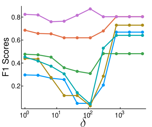
We additionally consider how different hypergraph splitting functions affect the output solution. We ran HyperLocal with the $\delta$-linear threshold splitting function for varying $\delta$ for a handful of clusters from both datasets, measuring the target cluster recovery F1 score (Fig. 3). We tested both integer and non-integer values of $\delta$, and found no meaningful difference in runtime. For the Stack Overflow hypergraph, HyperLocal’s performance plummets for $\delta$ near 100 and performance is maximized for very large $\delta$ (Fig. 3a). In contrast, for the Amazon hypergraph, the maximum F1 for each cluster is almost always obtained when $\delta=1.0$ (Fig. 3b). This suggests that if one has access to a subset of ground truth clusters in a hypergraph, running a similar set of experiments provides a simple and effective strategy for choosing a value of $\delta$ to use when searching for other, similar clusters.