Hilbert space average of transition probabilities

Consider a set of pure states $\{\ket{\phi}\}$ initially featuring very similar expectation values concerning an observable $M$. Then dynamical quantum typicality refers to the situation in which the majority of these states will also feature very similar expectation values to the same or another observable at any later time [1]. This statement holds true under quite general conditions as it is not even dependent on the details of the dynamics. A necessary requirement is that the dimension $N$ of the finite dimensional Hilbert space $\mathcal{H}$ is large. In [2] the construction of these sets was generalized and sufficient conditions were explored. It was found that besides a large Hilbert space dimension the preset expectation value $\braket{\phi|M|\phi}$ as well as the spectrum of $M$ play an important role.

The tool to develop these findings is the Hilbert space averaging method [3]. With its aid one can establish the average of a function depending on pure states, e.g. the expectation value of some arbitrary observable. The standard deviation as the square root of the Hilbert space variance describes the width of the distribution of the states around this value and is found to be small if certain conditions are met [2]. Using these methods it was possible to get more insight into the eigenstate thermalization hypothesis (ETH) [4, 5, 6, 7], that strives to explain the thermalization of isolated quantum systems. Furthermore the resulting identities have been utilized as a computational scheme, e.g. to calculate spin-correlations [8, 9, 10, 11] as well as in the case of out-of-time-ordered correlations (OTOC’s) [12], which are able to diagnose many- body localized phases [13]. The intention of the present work is to extend the Hilbert space averaging method and open it up to new possibilities by studying the transition probabilities $\left|\braket{\chi|A|\psi}\right|^{2}$ of an arbitrary operator $A$.

On the technical level this averaging procedure is closely connected to the concept of random matrix theory [14, 15]. This method substitutes the matrices, relevant for the description of the system (e.g. the Hamiltonian, scattering matrix etc.), by random matrices. It was applied quite successfully to systems sharing a sufficiently high amount of complexity. The only information about the system entering the model are its symmetries, revealing universal system features exclusively depending on the symmetry class. In previous works, where concepts of random matrix theory have been applied to study transition probabilities [16, 17, 18, 19] the components of the states were drawn from a Gaussian distribution with zero mean, implying statistical orthogonality of the states in high dimensions. Thus, these states are able to model the eigenstates of an observable and the transition probability between those eigenstates. A well known result of this approach is the Porter-Thomas distribution [20, 21], which determines the statistics of the transition probabilities in the case of time reversal symmetry. However, in this paper we follow a new route, where we explicitly choose the overlap of the deployed states, putting the assumption of statistical orthogonality aside. The situation of nonorthogonal states is relevant, when states, that are not eigenstates of the Hamiltonian or another observable, important for the system description, are prepared. For example within the doorway mechanism (see [22, 23] and references therein) a distinct state (the so-called doorway state), that is not an eigenstate of the Hamiltonian, but is distinguished by another feature (e.g. collective motion in many-body systems) is coupled to a background of states, that are not orthogonal to the doorway state. This mechanism has far reaching applications in nuclear physics (giant multipole resonance) [24], molecular physics [25, 26] and mesoscopic physics [27, 28].

The outline of the paper is as follows: in section 2 we will introduce the Hilbert space averaging method and give a short review on the concept of quantum typicality, focusing especially on the construction of typical states and on the aforementioned conditions of dynamical quantum typicality. In section 3 we will shortly introduce the model on which we present our findings. In section 4 we approach the Hilbert space average of transition probabilities, first without imposing any further condition onto the states, and then after fixing the initial overlap of the involved states. We demonstrate and interpret our results with the aid of numerical calculations in section 5. More involved analytical calculations are relegated to the appendix.

We restrict ourselves to a finite dimensional Hilbert space $\mathcal{H}=\mathbb{C}^{N}$ with dimension $N$. In practice this will be due to the nature of the system or because of conserved quantities, e.g. the Hilbert space could be the energy shell of an isolated system. We now give an overview of the concept of quantum typicality.

We want to find the average value of a function $f:\mathcal{H}\rightarrow\mathbb{C}$. This is the Hilbert space average [3]

$${\text{HA}}\left[f(\psi)\right]=\frac{\int d[\psi]f(\psi)\delta(\braket{\psi|\psi}-1)}{\int d[\psi]\delta(\braket{\psi|\psi}-1)}.$$

(2.1)

Thus, we choose normalized vectors as representative for the state, which allows us to restrict our integration to the unit sphere in $\mathcal{H}=\mathbb{C}^{N}$. Then we normalize this integral by the volume of the unit sphere.

We note that for a normalized vector there is still a relative phase $e^{i\lambda}$ left as a degree of freedom. However, the functions, treated on the next pages, fulfill $\forall\lambda\in[0,2\pi):f(\psi)=f(e^{i\lambda}\psi)$ (in other words they are $U(1)$ invariant) and our normalization makes up for that multiple occurrence of identical states in the integral over the sphere $S^{2N-1}$. The latter can be seen as a fibre bundle $S^{2N-1}\sim\mathbb{C}P^{N-1}\times U(1)$, whose base manifold is the complex projective space $\mathbb{C}P^{N-1}$, that is the space of all rays in $\mathbb{C}^{N}$ [29]. Likewise the Hilbert space variance can be defined as

$${\text{HV}}[f(\psi)]={\text{HA}}\left[f^{2}(\psi)\right]-{\text{HA}}^{2}\left[f(\psi)\right].$$

(2.2)

A first important application is the expectation value of an operator $M$. As shown in [3] this can be obtained without using the explicit form of (2.1). Because the integration regime is invariant under the action of the unitary group $U(N)$ (this is also known as Haar measure [29]) we can choose an arbitrary orthonormal basis $\{\ket{i}\}$ to represent our states and then use the linearity of the Hilbert space average

$${\text{HA}}\left[\braket{\psi|M|\psi}\right]=\sum_{i,j}M_{ij}\ {\text{HA}}\left[\psi_{i}^{*}\psi_{j}\right]$$

(2.3)

with the coordinates $\psi_{i}=\braket{i|\psi}$. The unit sphere is invariant under $\psi_{i}\rightarrow-\psi_{i}$ for all $i$ and therefore the average will vanish for $i\neq j$. Now we can use the normalization of our states

$${\text{HA}}\left[\sum_{i}\left|\psi_{i}\right|^{2}\right]=\sum_{i}{\text{HA}}\left[\left|\psi_{i}\right|^{2}\right]=1$$

(2.4)

to conclude

$${\text{HA}}\left[\left|\psi_{i}\right|^{2}\right]=\frac{1}{N}$$

(2.5)

and

$${\text{HA}}\left[\braket{\psi|M|\psi}\right]=\frac{{\text{Tr}}\ M}{N}.$$

(2.6)

The Hilbert space variance of the expectation value is [3]

$${\text{HV}}\left[\braket{\psi|M|\psi}\right]=\frac{1}{N+1}\left(\frac{{\text{Tr}}\ M^{2}}{N}-\frac{{\text{Tr}}^{2}M}{N^{2}}\right).$$

(2.7)

A sharp Hilbert space average, in the sense that the standard deviation drops faster in $N$ than the average, can be reached by demanding constant spectral moments ${\text{Tr}}\ M/N$ and ${\text{Tr}}\ M^{2}/N$ [1]. The calculation of higher moments of $\braket{\psi|M|\psi}$ is more complicated. In appendix A.2 we present a formula, that achieves this for positive integer powers.

Next we will review the typicality results of [2] and choose $M$ as an observable. Reimann constructs a statistical operator

$$\rho(m,M)=\frac{1}{N}\frac{1}{1+y(m-M)},$$

(2.8)

where $m$ is the desired expectation value of $\rho(m,M)$ concerning $M$. The parameter $y\in\mathbb{R}$ is chosen so that the normalization ${\text{Tr}}\ \rho=1$ and ${\text{Tr}}\ M\rho=m$ are fulfilled, and is determined by the roots of a rational function. The states

$$\ket{\phi}:=\Lambda\ket{\psi},$$

(2.9)

where we use the abbreviation $\Lambda=\sqrt{N\rho}$, exhibit the desired preset expectation value $m$ as their Hilbert space average

$${\text{HA}}\left[\braket{\phi|M|\phi}\right]={\text{HA}}\left[\braket{\psi|\Lambda M\Lambda|\psi}\right]={\text{Tr}}\ M\rho=m.$$

(2.10)

They are not necessarily normalized, but in average they are

$${\text{HA}}\left[\braket{\phi|\phi}\right]={\text{HA}}\left[\braket{\psi|\Lambda^{2}|\psi}\right]={\text{Tr}}\ \rho=1.$$

(2.11)

The Hilbert space variance indicates how much one can trust these results in the case of an individual $\ket{\phi}$. The purity

$$P={\text{Tr}}\ \rho^{2}$$

(2.12)

is an upper bound for the variances

$${\text{HV}}\left[\braket{\phi|\phi}\right]=\frac{NP-1}{N+1}\leq P\qquad\text{and}\qquad{\text{HV}}\left[\braket{\phi|M|\phi}\right]\leq\left\lVert M\right\rVert^{2}P,$$

(2.13)

where the operator norm $\left\lVert M\right\rVert$ is defined as the absolute value of the largest eigenvalue in modulus. Therefore one achieves typicality if the purity is low $P\ll 1$. While a large Hilbert space is a prerequisite for low purity, due to (2.8) $P$ is also strongly dependent on the observable $M$ and the expectation value $m$. As an example consider the magnetization in $z$-direction

$$M_{z}=\sum_{i=1}^{n}\sigma_{i}^{z}$$

(2.14)

of an $n$-particle spin-1/2 chain (cf. section 3). In this case the eigenvalues of the local spin observables $\sigma_{i}^{z}$ are $\pm 1$. Therefore the eigenvalue density of $M_{z}$ is a binomial distribution, i.e. there are only few eigenstates near the maximal resp. minimal magnetization of $\pm n$, while the majority is located around a magnetization of zero in the center. In fact, there is only a single state that has the maximal resp. minimal magnetization as its expectation value, making it highly untypical. This leads to a high purity of statistical operators with expectation values near those values. It is exactly the other way around for statistical operators with ${\text{Tr}}\ \rho M_{z}\approx 0$.

Finally we note that the above equations remain valid if $M$ is replaced by any other observable $B(t)$, that does not fulfill (2.10). Thus, dynamical quantum typicality is retrieved, namely that states $\{\ket{\phi}\}$ initially featuring $\braket{\phi|M|\phi}\approx m$ with small variance will also center around a common expectation value for another observable $B$ with small variance. As the deployed observables enter only in terms of their operator norm, the upper bound of the variance (2.13) is time independent for unitary time evolution.

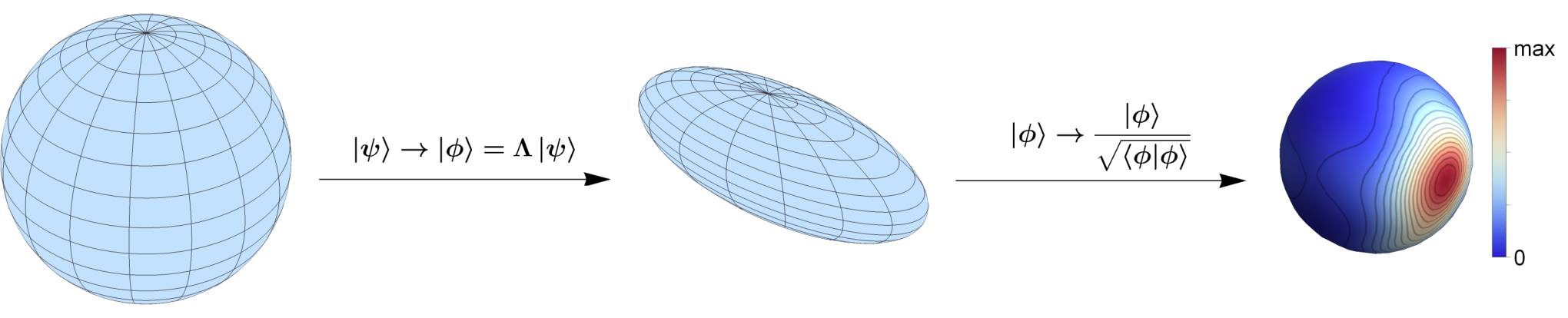
We want to give a geometrical interpretation of what is done here, illustrated in Fig. 1 for $N=3$. We uniformly sampled 100 vectors (in $\mathbb{R}^{3}$) on the unit sphere and applied $\Lambda$ with random positive eigenvalues of $\rho$, so that ${\text{Tr}}\ \rho=1$. Because $\Lambda$ is positive and Hermitian one can comprehend it as the deformation of the former integration regime (the unit sphere) into an ellipsoid. The new states $\{\ket{\phi}\}$ are still uniformly distributed, but now over the ellipsoid. This ellipsoid is then described by the quadric $\braket{\psi|\Lambda^{-2}|\psi}-1=0$. A subsequent normalization of each state will generate a nonuniform probability distribution on the unit sphere, which is given by the norm of the states on the surface of the ellipsoid $p(\psi):=\left\lVert\Lambda\ket{\psi}\right\rVert$. In practice we interpolated our data [30] to generate the density plot shown in the figure. We want to make a short remark about (2.9). Inserting the fully mixed state $\rho_{\text{{m}}}=1\!\!1/N$ (the one with the lowest purity) yields the uniform distribution from which we drew the states $\ket{\psi}$.

Now we introduce the model, on which we want to present the findings of the next section. The kicked Ising chain (KIC) is a many-body quantum system that entails rich dynamics, reaching from integrable to fully chaotic. It consists of a closed ring of $n$ spins (here spin-1/2 thus the Hilbert space dimension is $N=2^{n}$) with nearest neighbour interaction and an on site magnetic field. Additionally the system is periodically kicked by a transverse magnetic field leading to a discretized time evolution. The Hamiltonian is thus a sum of two parts

$$H=H_{I}+H_{K}\sum_{\tau=-\infty}^{\infty}\delta(t-\tau).$$

(3.1)

The interaction part is

$$H_{I}=\sum_{i=1}^{n}\left(J\sigma_{i}^{z}\sigma_{i+1}^{z}+h\ \sigma_{i}^{z}\right),$$

(3.2)

where $J$ is the coupling strength and $h$ the on site magnetic field. The kick part is

$$H_{K}=\sum_{i=1}^{n}b\ \sigma_{i}^{x}$$

(3.3)

with the transverse magnetic field $b$. In the present case of a spin-1/2 chain, $\sigma_{i}^{\alpha}$ with $\alpha\in\{x,y,z\}$ are the Pauli matrices acting at site $i$. Due to the boundary condition we have $\sigma^{\alpha}_{i}=\sigma^{\alpha}_{i+n}$. The time evolution operator for one period (Floquet operator) also splits in two parts and is given by

$$U=\mathcal{T}\ {\text{Exp}}\left[-i\int_{0}^{1}H(t)dt\right]=U_{I}U_{K}$$

(3.4)

with

$$U_{I}={\text{Exp}}\left[-iH_{I}\right],\qquad U_{K}={\text{Exp}}\left[-iH_{K}\right]$$

(3.5)

and the time ordering operator $\mathcal{T}$. Here we use units in which $\hbar=1$. The system becomes integrable for $b=0$ as the Hamiltonian will be diagonal in the basis of $\sigma^{z}$ and also if $h=0$. In the latter case it can be mapped onto a chain of noninteracting spinless fermions via a Jordan-Wigner transformation [31, 32].

In quantum chaos [33, 34] the spectral statistics of the operators governing the dynamics, i.e. the Hamiltonian and the time evolution operator, is used to identify regular and chaotic behaviour. In this context the spectral form factor

$$K(T)=\frac{\left|{\text{Tr}}\ U^{T}\right|^{2}}{N}$$

(3.6)

is a popular quantity. In recent years the KIC form factor was well examined [32, 35, 36]. We will reconsider it in section 5, where we find a connection between spectral statistics and the Hilbert space average.

We now turn to transition probabilities $\left|\braket{\chi|A|\psi}\right|^{2}$ describing the probability to find $\ket{\psi}$ in $\ket{\chi}$ after applying an arbitrary operator $A$. Assuming again that $\ket{\psi}$ is random uniformly distributed the Hilbert space average evaluates to

$${\text{HA}}_{\psi}\left[\left|\braket{\chi|A|\psi}\right|^{2}\right]={\text{HA}}_{\psi}\left[\braket{\psi|\left(A^{\dagger}\ket{\chi}\bra{\chi}A\right)|\psi}\right]=\frac{{\text{Tr}}\ A^{\dagger}\ket{\chi}\bra{\chi}A}{N}=\frac{\braket{\chi|AA^{\dagger}|\chi}}{N}.$$

(4.1)

Here we used (2.6) and henceforth we indicate which state will be averaged by a subscript if ambiguities cannot be excluded. The order of $A$ and its adjoint operator on the right hand side changes if $\ket{\psi}$ and $\ket{\chi}$ on the left hand side are interchanged. This can be disregarded if $A$ commutes with its adjoint which is the case for Hermitian or unitary operators.

To understand this result, it helps to consider, for the time being, a unitary operator $A$, which does not change the relative orientation of the states and thus has no effect on their distribution. Then the average probability to find $\ket{\psi}$ parallel to one of the $N$ axes of the vector space is

$${\text{HA}}_{\psi}\left[\left|\braket{\chi|A|\psi}\right|^{2}\right]=\frac{1}{N},$$

(4.2)

leading to their statistical orthogonality in the case of large $N$. Returning to a general operator $A$ we can average the remaining state $\ket{\chi}$ and arrive at

$${\text{HA}}_{\psi,\chi}\left[\left|\braket{\chi|A|\psi}\right|^{2}\right]={\text{HA}}_{\chi}\left[\frac{\braket{\chi|AA^{\dagger}|\chi}}{N}\right]=\frac{{\text{Tr}}\ AA^{\dagger}}{N^{2}}.$$

(4.3)

Endowing $\ket{\psi}$ as well as $\ket{\chi}$ with $\Lambda=\sqrt{N\rho}$ and $\Lambda^{\prime}=\sqrt{N\rho^{\prime}}$, where $\rho$ and $\rho^{\prime}$ are arbitrary statistical operators, like in (2.9) we find

$${\text{HA}}_{\psi,\chi}\left[\left|\braket{\chi|\Lambda^{\prime}A\Lambda|\psi}\right|^{2}\right]={\text{Tr}}\ \rho^{\prime}A\rho A^{\dagger}$$

(4.4)

and especially for $\rho^{\prime}=\rho$ and $A=1\!\!1$

$${\text{HA}}_{\psi,\chi}\left[\left|\braket{\chi|\Lambda^{2}|\psi}\right|^{2}\right]=P.$$

(4.5)

Comparing (4.2) and (4.5) this motivates the effective dimension

$$d_{\text{eff}}:=\frac{1}{P}$$

(4.6)

used by various authors [4, 37], which describes the variety of different states appearing in the mixture $\rho$. Applying (2.7) for the corresponding Hilbert space variances yields

	$\displaystyle{\text{HV}}_{\psi}\left[\left|\braket{\chi|A|\psi}\right|^{2}\right]$	$\displaystyle=\frac{N-1}{N^{2}(N+1)}\braket{\chi|AA^{\dagger}|\chi}^{2}$		(4.7)
	$\displaystyle{\text{HV}}_{\psi,\chi}\left[\left|\braket{\chi|A|\psi}\right|^{2}\right]$	$\displaystyle=\frac{N-1}{N^{3}(N+1)^{2}}\left({\text{Tr}}\left(AA^{\dagger}\right)^{2}+{\text{Tr}}^{2}AA^{\dagger}\right).$

In the remaining part of the paper we will put the statistical orthogonality, revealed in (4.2), aside by fixing the overlap of $\ket{\psi}$ and $\ket{\chi}$ to an arbitrary complex number $z=\braket{\chi|\psi}$ within the unit circle ($\left|z\right|\leq 1$). We do this by adding the corresponding $\delta$-function into the Hilbert space average. As its argument is complex, it has to be understood in terms of a product of two $\delta$-functions concerning the real and imaginary parts. Initially, we want to keep $\ket{\chi}$ fixed, which leads to the following expression

$\displaystyle{\text{HA}}_{\psi}\left[\left|\braket{\chi|A|\psi}\right|^{2}\delta(\braket{\chi|\psi}-z)\right]$

$\displaystyle=\frac{1-\left|z\right|^{2}}{N-1}\braket{\chi|AA^{\dagger}|\chi}+\frac{N\left|z\right|^{2}-1}{N-1}\left|\braket{\chi|A|\chi}\right|^{2}.$

(4.8)

A detailed derivation of this and also the following results is found in appendix A.1. We may now average over the remaining state using the formulae of appendix A.2

$${\text{HA}}_{\psi,\chi}\left[\left|\braket{\chi|A|\psi}\right|^{2}\delta(\braket{\chi|\psi}-z)\right]=\frac{N-\left|z\right|^{2}}{N^{3}-N}{\text{Tr}}\ AA^{{\dagger}}+\frac{N\left|z\right|^{2}-1}{N^{3}-N}\left|{\text{Tr}}\ A\right|^{2}.$$

(4.9)

While the former results are valid for uniformly distributed $\ket{\psi}$, we are also interested in the nonuniform case according to section 2. To this end we use

$$\ket{\psi}\rightarrow\Lambda\ket{\psi}.$$

(4.10)

In general $\Lambda\ket{\psi}$ is not normalized. Thus, we normalize the argument of $\delta\left(\braket{\chi|\Lambda|\psi}-z\right)$ by $\left\lVert\Lambda\ket{\chi}\right\rVert=\sqrt{\braket{\chi|\Lambda^{2}|\chi}}$. This is possible due to the Hermiticity of $\Lambda$. Furthermore as the normalization is not dependent on $\ket{\psi}$, we use the scaling property of the $\delta$-function

$$\delta\left(\frac{\braket{\chi|\Lambda|\psi}}{\sqrt{\braket{\chi|\Lambda^{2}|\chi}}}-z\right)=\sqrt{\braket{\chi|\Lambda^{2}|\chi}}\ \delta\left(\braket{\chi|\Lambda|\psi}-z\sqrt{\braket{\chi|\Lambda^{2}|\chi}}\right).$$

(4.11)

In this way we extracted the $\Lambda$-dependence of the absolute value of $\braket{\chi|\Lambda|\psi}$ and are able to retain our choice $\left|z\right|\leq 1$ by rescaling. The square root prefactor is cancelled by the normalization, for details see appendix A.1. Therefore we arrive at an integral which is equivalent to (4.8) for nonuniformly distributed $\ket{\psi}$

$${\text{HA}}_{\psi}\left[\left|\braket{\chi|A\Lambda|\psi}\right|^{2}\delta\left(\frac{\braket{\chi|\Lambda|\psi}}{\sqrt{\braket{\chi|\Lambda^{2}|\chi}}}-z\right)\right]=\frac{1-\left|z\right|^{2}}{N-1}\braket{\chi|A\Lambda^{2}A^{\dagger}|\chi}+\frac{N\left|z\right|^{2}-1}{N-1}\frac{\left|\braket{\chi|A\Lambda^{2}|\chi}\right|^{2}}{\braket{\chi|\Lambda^{2}|\chi}}.$$

(4.12)

It turns out that a subsequent averaging over $\ket{\chi}$ is more difficult than in the uniform case. This is because of the fraction in the second term of (4.12). We treat it with an approximation at the very end of the next section (cf. (5.2)), where we demonstrate our results numerically. For this purpose we will also calculate the variances of the here presented cases.

Our numerical demonstration is based upon the KIC model introduced in section 3. The transition probability for individual, randomly sampled $\ket{\chi}$ and $\ket{\psi}$ after action of the KIC Floquet operator (3.4) is shown. The unitarity $UU^{\dagger}=U^{\dagger}U=1\!\!1$ of the Floquet operator leads to slight simplifications of (4.8), (4.9) and (4.12). We will first deal with states, that are uniformly distributed under the imposed conditions. Subsequently, we prepare our states such that they feature a given expectation value of the magnetization (2.14), which yields a nonuniform distribution.

References

- [1] C. Bartsch, J. Gemmer. Phys. Rev. Lett. 102 110403 (2009).
- [2] P. Reimann. Phys. Rev. E 97 062129 (2018).
- [3] J. Gemmer, M. Michel, G. Mahler. Quantum Thermodynamics. Springer-Verlag Berlin Heidelberg (2009).
- [4] P. Reimann. Phys. Rev. Lett. 120 230601 (2018).
- [5] R. Steinigeweg, A. Khodja, H. Niemeyer, C. Gogolin, J. Gemmer. Phys. Rev. Lett. 112 130403 (2014).
- [6] A. Khodja, R. Steinigeweg, J. Gemmer. Phys. Rev. E 91 012120 (2015).
- [7] R. Steinigeweg, J. Herbrych, P. Prelovšek. Phys. Rev. E 87 012118 (2013).
- [8] R. Steinigeweg, J. Gemmer, W. Brenig. Phys. Rev. Lett. 112 120601 (2014).
- [9] R. Steinigeweg, J. Herbrych, F. Pollmann, W. Brenig. Phys. Rev. B 94 180401 (2016).
- [10] T. A. Elsayed, B. V. Fine. Phys. Rev. Lett. 110 070404 (2013).
- [11] J. Richter, R. Steinigeweg. Phys. Rev. B 99 094419 (2019).
- [12] I. Kukuljan, S. Grozdanov, T. Prosen. Phys. Rev. B 96 060301 (2017).
- [13] X. Chen, T. Zhou, D. A. Huse, E. Fradkin. Annalen der Physik 529 7 1600332 (2017).
- [14] T. Guhr, A. Müller-Groeling, H. A. Weidenmüller. Phys. Rep. 299 4 189–425 (1998).
- [15] M. L. Mehta. Random Matrices. Academic Press (2004).
- [16] C. I. Barbosa, T. Guhr, H. L. Harney. Phys. Rev. E 62 1936–1949 (2000).
- [17] A. Hamoudi, R. G. Nazmitdinov, E. Shahaliev, Y. Alhassid. Phys. Rev. C 65 064311 (2002).
- [18] N. Ullah. Journal of Mathematical Physics 4 10 1279–1282 (1963).
- [19] N. Ullah. Journal of Mathematical Physics 8 5 1095–1096 (1967).
- [20] C. E. Porter, R. G. Thomas. Phys. Rev. 104 483–491 (1956).
- [21] Y. Alhassid, R. D. Levine. Phys. Rev. Lett. 57 2879–2882 (1986).
- [22] H. Kohler, T. Guhr, S. Åberg. New Journal of Physics 12 7 073026 (2010).
- [23] H. Kohler, H.-J. Sommers, S. Åberg, T. Guhr. Phys. Rev. E 81 050103 (2010).
- [24] V. Zelevinsky. Annual Review of Nuclear and Particle Science 46 1 237–279 (1996).
- [25] I. Kawata, H. Kono, Y. Fujimura, A. D. Bandrauk. Phys. Rev. A 62 031401 (2000).
- [26] E. Peyroula, R. Jost, M. Lombardi, P. Dupré. Chemical Physics 102 3 417 – 435 (1986).
- [27] S. Åberg, T. Guhr, M. Miski-Oglu, A. Richter. Phys. Rev. Lett. 100 204101 (2008).
- [28] M. Hussein, V. Kharchenko, L. Canto, R. Donangelo. Annals of Physics 284 1 178 – 194 (2000).
- [29] I. Bengtsson, K. Zyczkowski. Geometry of Quantum States: An Introduction to Quantum Entanglement. Cambridge University Press (2006).
- [30] P. J. Diggle, N. I. Fisher. Computers & Geosciences 11 6 725–766 (1985).
- [31] E. Lieb, T. Schultz, D. Mattis. Ann. Phys. 16 3 407–466 (1961).
- [32] M. Akila, D. Waltner, B. Gutkin, T. Guhr. J. Phys. A 49 37 375101 (2016).
- [33] H.-J. Stöckmann. Quantum Chaos - an introduction. Cambridge University Press (1999).
- [34] F. Haake. Quantum Signatures of Chaos. Springer-Verlag Berlin Heidelberg (2010).
- [35] B. Bertini, P. Kos, T. Prosen. Phys. Rev. Lett. 121 264101 (2018).
- [36] P. Braun, D. Waltner, M. Akila, B. Gutkin, T. Guhr. arXiv:1902.06265 (2019).
- [37] N. Linden, S. Popescu, A. J. Short, A. Winter. Phys. Rev. E 79 061103 (2009).
- [38] K. Scharnhorst. Acta Applicandae Mathematica 69 1 95–103 (2001).
- [39] J. M. Luck. J. Phys. A 49 11 115303 (2016).
- [40] J. M. Luck. J. Phys. A 50 35 355301 (2017).
- [41] I. N. Sneddon. The use of integral transforms. McGraw-Hill Book Company (1972).