跳到论文正文
W Papers独立论文阅读器 arXiv:2002.09385 论文正文 计算阅读时间 · 0%
引用这篇论文根据当前论文元数据生成,正式投稿前建议核对。


License: arXiv.org perpetual non-exclusive license
arXiv:2002.09385v1 [math.NA] 21 Feb 2020

Consistency and convergence for a family of finite volume discretizations of the Fokker–Planck operatorThanks: M. H. and A. S. are financed by Deutsche Forschungsgemeinschaft (DFG) through Grant CRC 1114 “Scaling Cascades in Complex Systems”, Project C05 Effective models for materials and interfaces with multiple scales. The work of M. K. received funding from the DFG under Germany’s Excellence Strategy – EXC2046: Math+ (Berlin Mathematics Research Center).

Martin Heida, Markus Kantner, Artur Stephan Address: Weierstrass Institute, Mohrenstr. 39, 10117 Berlin, Germany Email address: martin.heida@wias-berlin.de Email address: markus.kantner@wias-berlin.de Email address: artur.stephan@wias-berlin.de
Abstract.

We introduce a family of various finite volume discretization schemes for the Fokker–Planck operator, which are characterized by different weight functions on the edges. This family particularly includes the well-established Scharfetter–Gummel discretization as well as the recently developed square-root approximation (SQRA) scheme. We motivate this family of discretizations both from the numerical and the modeling point of view and provide a uniform consistency and error analysis. Our main results state that the convergence order primarily depends on the quality of the mesh and in second place on the quality of the weights. We show by numerical experiments that for small gradients the choice of the optimal representative of the discretization family is highly non-trivial while for large gradients the Scharfetter–Gummel scheme stands out compared to the others.

Key words and phrases: 
Finite Volume, Fokker–Planck, Scharfetter–Gummel, Stolarsky mean, Consistency, Order of Convergence
2010 Mathematics Subject Classification
35Q84,49M25,65N08

1. Introduction

The Fokker–Planck equation (FPE), also known as Smoluchowski equation or Kolmogorov forward equation, is one of the major equations in theoretical physics and applied mathematics. It describes the time evolution of the probability density function of a particle in an external force field (e.g., fluctuating forces as in Brownian motion). The equation can be generalized to other contexts and observables and has been employed in a broad range of applications, including physical chemistry, protein synthesis, plasma physics and semiconductor device simulation. Thus, there is a huge interest in the development of efficient and robust numerical methods. In the context of finite volume (FV) methods, the central objective is a robust and accurate discretization of the (particle or probability) flux implied by the FPE.

A particularly important discretization scheme for the flux was derived by Scharfetter and Gummel [SG69] in the context of the drift-diffusion model for electronic charge carrier transport in bipolar semiconductor devices [vR50]. The typically exponentially varying carrier densities at p-n junctions lead to unphysical results (spurious oscillations), if the flux is discretized in a naive way using standard finite difference schemes [MW94]. The problem was overcome by considering the flux expression as a one-dimensional boundary value problem along each edge between adjacent mesh nodes. The resulting Scharfetter–Gummel (SG) scheme provides a robust discretization of the flux as it asymptotically approaches the numerically stable discretizations in the drift- (upwind scheme) and diffusion-dominated (central finite difference scheme) limits. The SG-scheme and its several generalizations to more complex physical problem settings are nowadays widely used in semiconductor device simulation [Mar86, FRD+17] and have been extensively studied in the literature [BMP89, EFG06, FKF17, Kan20]. The SG-scheme is also known as exponential fitting scheme and was independently discovered by Allan and Southwell [AS55] and Il’in [Il’69] in different contexts.

Recently, an alternative flux discretization method, called square-root approximation (SQRA) scheme, has been derived explicitly for high dimensional problems. The original derivation in [LFW13] aims at applications in molecular dynamics and is based on Markov state models. However, it can also be obtained from a maximum entropy path principle [DJSD15] and from discretizing the Jordan–Kinderlehrer–Otto variational formulation of the FPE [Mie13a]. In Section 3.3, we provide a derivation of SQRA scheme, which is motivated from the theory of gradient flows. In contrast to the SG-scheme, the SQRA is very recent and only sparsely investigated. The only contributions on the convergence seem to be [Mie13a] in 1D, [DHWK] (formally, rectangular meshes) and [Hei18] using G-convergence.

The SG and the SQRA schemes both turn out to be special cases of a family of discretization schemes based on weighted Stolarsky means, see Section 3.2. This family is very rich and allows for a general convergence and consistency analysis, which we carry out in Sections 4–5. Interestingly, there seems to be no previous results in the literature.

1.1. The FPE and the SG and SQRA discretization schemes

In this work, we consider the stationary Fokker–Planck equation

(1.1) −∇⋅(κ∇u)−∇⋅(κu∇V)=f,-\nabla\cdot\left(\kappa\nabla u\right)-\nabla\cdot\left(\kappa u\nabla V\right)=f,

which can be equivalently written as

div𝐉⁡(u,V)=f\mathop{\mathrm{div}}\mathbf{J}(u,V)=f

using the flux 𝐉(u,V)=−κ(∇u+u∇V)\mathbf{J}(u,V)=-\kappa\left(\nabla u+u\nabla V\right), where κ>0\kappa>0 is a (possibly space-dependent) diffusion coefficient and V:Ω→ℝV:\Omega\rightarrow\mathbb{R} is a given potential. The flux 𝐉\mathbf{J} consists of a diffusive part κ∇u\kappa\nabla u and a drift part κu∇V\kappa u\nabla V, which compensate for the stationary density π=e−V\pi=\mathrm{{e}}^{-V} (also known as the Boltzmann distribution) as 𝐉⁡(e−V,V)=0\mathbf{J}(\mathrm{{e}}^{-V},V)=0. This reflects the principle of detailed balance in the thermodynamic equilibrium. The right-hand side ff describes possible sink or source terms.

The SG and the SQRA schemes of the Fokker–Planck operator div​𝐉​(u,V)\mathrm{div}\,\mathbf{J}(u,V) that are considered below are given in the form

(1.2) (ℱB𝒯u)i:=−∑j:i∼jmi​jhi​jκi​j(B(Vi,Vj)uj−B(Vj,Vi)ui),\left(\mathcal{F}_{B}^{\mathcal{T}}u\right)_{i}:=-\sum_{j:\,i\sim j}\frac{m_{ij}}{h_{ij}}\kappa_{ij}\left(B\left(V_{i},V_{j}\right)u_{j}-B\left(V_{j},V_{i}\right)u_{i}\right),

where ∑j:j∼i\sum_{j:\,j\sim i} indicates a sum over all cells adjacent to the ii-th cell of the mesh, mi​jm_{ij} is the mass of the interface between the ii-th and jj-th cell, hi​jh_{ij} is the distance between the corresponding nodes and κi​j\kappa_{ij} is the discretized diffusion coefficient κ\kappa. We are particularly interested in the two cases

(1.3) B⁡(Vi,Vj)\displaystyle B\left(V_{i},V_{j}\right) =B1​(Vi−Vj):=Vi−VjeVi−Vj−1\displaystyle=B_{1}\left(V_{i}-V_{j}\right):=\frac{V_{i}-V_{j}}{\mathrm{{e}}^{V_{i}-V_{j}}-1}
(1.4) orB⁡(Vi,Vj)\displaystyle\text{or}\quad B\left(V_{i},V_{j}\right) =B2​(Vi−Vj):=e−12​(Vi−Vj)\displaystyle=B_{2}\left(V_{i}-V_{j}\right):=\mathrm{{e}}^{-\frac{1}{2}\left(V_{i}-V_{j}\right)}

with either the Bernoulli function B1B_{1} (for SG) or with the SQRA-coefficient B2B_{2}. The schemes are derived under the assumption of constant flux, diffusion constant and potential gradient along the respective edges.

In the pure diffusion regime, i.e., for Vi−Vj→0V_{i}-V_{j}\to 0, the Bernoulli function provides B1​(Vi−Vj)→1B_{1}\left(V_{i}-V_{j}\right)\rightarrow 1, such that the SG scheme approaches a discrete analogue of the diffusive part of the continuous flux: Ji​j=κi​j​(ui−uj)/hi​jJ_{ij}=\kappa_{ij}(u_{i}-u_{j})/h_{ij}. In the drift-dominated regime, i.e., for Vj−Vi→±∞V_{j}-V_{i}\rightarrow\pm\infty, the asymptotics of B1B_{1} recover the upwind scheme

(1.5) Ji,j→−κi,j​Vj−Vihi,j​{ujif ​Vj>Viuiif ​Vj<Vi,J_{i,j}\to-\kappa_{i,j}\frac{V_{j}-V_{i}}{h_{i,j}}\begin{cases}u_{j}&\text{if }V_{j}>V_{i}\\ u_{i}&\text{if }V_{j}<V_{i}\end{cases},

which is a robust discretization of the drift part of the flux, where the density uu is evaluated in the donor cell of the flux. Hence, the Bernoulli function B1B_{1} interpolates between the appropriate discretizations for the drift- and diffusion-dominated limits, which is why the SG scheme is the preferred FV scheme for Fokker–Planck type operators. Indeed, the SQRA scheme is consistent with the diffusive limit, but is less accurate than the SG scheme in the case of strong gradients ∇V\nabla V.

1.2. The Stolarsky mean approximation schemes

In this work, we investigate the relative L2L^{2}-distance between the discrete SQRA and SG solutions on the same mesh and the order of convergence of the SQRA scheme, which was an open problem. It turns out that both methods are members of a broad family of finite volume discretizations that stem from the weighted Stolarsky means

Sα,β​(x,y)=(β⁡(xα−yα)α⁡(xβ−yβ))1α−β,S_{\alpha,\beta}\left(x,y\right)=\left(\frac{\beta\left(x^{\alpha}-y^{\alpha}\right)}{\alpha\left(x^{\beta}-y^{\beta}\right)}\right)^{\frac{1}{\alpha-\beta}},

see Section 3.2. We benefit from the general structure of these schemes and prove order of convergence on consistent meshes in the sense of the recent work [DPD18]. We will see that the error naturally splits into the consistency error for the discretization of the Laplace operator plus an error which is due to the discretization of the stationary solution π\pi and the Stolarsky mean, see Theorem 5.4.

We will demonstrate below that the Stolarsky discretization schemes for (1.1) read

(1.6) −∑j:j∼imi​jhi​jκi​jSi​j(ujπj−uiπi)\displaystyle-\sum_{j:\,j\sim i}\frac{m_{ij}}{h_{ij}}\kappa_{ij}S_{ij}\left(\frac{u_{j}}{\pi_{j}}-\frac{u_{i}}{\pi_{i}}\right) =fi,\displaystyle=f_{i},

where πi=e−Vi\pi_{i}=\mathrm{{e}}^{-V_{i}} , fi=∫Ωiff_{i}=\int_{\Omega_{i}}f is the integral of ff over the ii-th cell and Si​j=Sα,β​(πi,πj)S_{ij}=S_{\alpha,\beta}\left(\pi_{i},\pi_{j}\right) is a Stolarsky mean of πi\pi_{i} and πj\pi_{j}. We sometimes refer to the general form (1.6) as discrete FPE.

The Stolarsky means Sα,βS_{\alpha,\beta} generalize Hölder means and other ff-means (see Table 2). An interesting aspect of the above representation is that all these schemes preserve positivity with the discrete linear operator being an MM-matrix. Furthermore, with the relative density U=u/πU=u/\pi we arrive at

−∑j:j∼imi​jhi​jκi​jSi​j(Uj−Ui)=fi,-\sum_{j:\,j\sim i}\frac{m_{ij}}{h_{ij}}\kappa_{ij}S_{ij}\left(U_{j}-U_{i}\right)=f_{i},

which is a discretization of the elliptic equation

−∇⋅(κπ∇U)=f,-\nabla\cdot\left(\kappa\pi\nabla U\right)=f,

where the discrete Fokker–Planck operator becomes a purely diffusive second order operator in UU. Furthermore, if κ\kappa is a symmetric strictly positive definite uniformly elliptic matrix, this operator is also symmetric strictly positive definite and uniformly elliptic. In the latter setting, we can thus rule out the occurrence of spurious oscillations in our discretization.

Although we treat the Stolarsky means as an explicit example, note that the main theorems also hold for other smooth means.

1.3. Major contributions of this work

Since we look at the FV discretization of the FPE from a very broad point of view, we summarize our major findings.

  • •

    We provide a derivation of the general Stolarsky mean FV discretization in Section 3.2.

  • •

    We discuss the gradient structure of the discretization schemes in view of the natural gradient structure of the FPE in Section 3.3.

  • •

    We provide order of convergence of the schemes as the fineness of the discretization tends to zero. In particular we show

    • –

      that the order of convergence is mainly determined by two independent parts: the consistency (Def. 2.7) of the mesh (Section 5.1) and an error due to the discretization of π\pi along the edge by the means S∗​(πi,πj)S_{\ast}(\pi_{i},\pi_{j}).

    • –

      that the order of convergence strongly depends on the constant α+β\alpha+\beta, where α\alpha and β\beta are the Stolarsky coefficients in Si​j=Sα,β​(πi,πj)S_{ij}=S_{\alpha,\beta}\left(\pi_{i},\pi_{j}\right) (Corollary 4.3).

    • –

      that the SG coefficients are to be preferred in regions of strong gradient ∇V\nabla V (Section 5.2).

1.4. Outlook

The results of this work suggest to search for “optimal” parameters α\alpha and β\beta in the choice of the Stolarsky mean in order to reduce the error of the approximation as much as possible. However, from an analytical point of view, the quest for such optimal α\alpha and β\beta is quite challenging. Moreover, since the optimal choice might vary locally, depending on the local properties of the potential VV, we suggest to implement a learning algorithm that provides suitable parameters α\alpha and β\beta depending on the local structure of VV and the mesh.

1.5. Outline of this work

After some preliminaries regarding notation and a priori estimates in Section 2, we will recall the classical derivation of the SG scheme in Section 3.1 and discuss its formal relation to SQRA. We will then provide a derivation of SQRA from physical principles in Section 3.3, based on the Jordan–Kinderlehrer–Otto [JKO98] formulation of the FPE. In Section 3.2, we show that SG and SQRA are elements of a huge family of discretization schemes (1.6).

Section 5 provides the error analysis and estimates for the consistency and the order of convergence. We distinguish the cases of small and large gradients and have a particular look at cubic meshes.

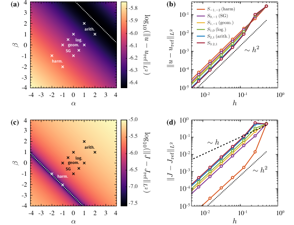
Finally, we show hat the optimal choice of S∗S_{\ast} depends on VV and ff but is not unique. If Sα,βS_{\alpha,\beta} denotes one of the Stolarsky means, we will prove in Section 4 that the Stolarsky means satisfying α+β=const\alpha+\beta=\mathrm{const} show similar quantitative convergence behavior as suggested in Corollary 4.3. Finally, this result is illustrated in Section 6 by numerical simulations.

2. Preliminaries and notation

We collect some concepts and notation, which will frequently be used in this work.

2.1. The Mesh

For a subset A⊂ℝdA\subset\mathbb{R}^{d}, A¯\overline{A} is the closure of AA.

Definition 2.1.

Let Ω⊂ℝd\Omega\subset\mathbb{R}^{d} be a polygonal domain. A finite volume mesh of Ω\Omega is a triangulation 𝒯=(𝒱,ℰ,𝒫)\mathcal{T}=(\mathcal{V},\mathcal{E},\mathcal{P}) consisting of a family of control volumes 𝒱:={Ωi,i=1,…,N}\mathcal{V}:=\left\{\Omega_{i},i=1,\dots,N\right\} which are convex polytope cells, a family of (d−1)\left(d-1\right)-dimensional interfaces

ℰ\displaystyle\mathcal{E} :=ℰΩ∪ℰ∂\displaystyle:=\mathcal{E}_{\Omega}\cup\mathcal{E_{\partial}}
ℰΩ\displaystyle\mathcal{E}_{\Omega} :={σi​j⊂ℝd:σi​j=∂Ωi∩∂Ωj}\displaystyle:=\left\{\sigma_{ij}\subset\mathbb{R}^{d}\,:\;\sigma_{ij}=\partial\Omega_{i}\cap\partial\Omega_{j}\right\}
ℰ∂\displaystyle\mathcal{E}_{\partial} :={σ⊂ℝd:σ=∂Ωi∩∂Ω​ is flat}\displaystyle:=\left\{\sigma\subset\mathbb{R}^{d}\,:\;\sigma=\partial\Omega_{i}\cap\partial\Omega\,\text{\ is flat}\right\}

and points 𝒫={xi,i=1,…,N}\mathcal{P}=\{x_{i},i=1,\dots,N\} with xi∈Ωi¯x_{i}\in\overline{\Omega_{i}} satisfying

  1. (i)

    ⋃iΩ¯i=Ω¯\bigcup_{i}\overline{\Omega}_{i}=\overline{\Omega}

  2. (ii)

    For every ii there exists ℰi⊂ℰ\mathcal{E}_{i}\subset\mathcal{E} such that Ω¯i\Ωi=⋃σ∈ℰiσ\overline{\Omega}_{i}\backslash\Omega_{i}=\bigcup_{\sigma\in\mathcal{E}_{i}}\sigma. Furthermore, ℰ=⋃iℰi\mathcal{E}=\bigcup_{i}\mathcal{E}_{i}.

  3. (iii)

    For every i,ji,j either Ω¯i∩Ω¯j=∅\overline{\Omega}_{i}\cap\overline{\Omega}_{j}=\emptyset or Ω¯i∩Ω¯j=σ¯\overline{\Omega}_{i}\cap\overline{\Omega}_{j}=\overline{\sigma} for σ∈ℰi∩ℰj\sigma\in\mathcal{E}_{i}\cap\mathcal{E}_{j} which will be denoted σi​j\sigma_{ij}.

The mesh is called hh-consistent if

  1. (iv)

    The Family (xi)i=1​…​N\left(x_{i}\right)_{i=1\dots N} is such that xi≠xjx_{i}\not=x_{j} if i≠ji\not=j and the straight line Di​jD_{ij} going through xix_{i} and xjx_{j} is orthogonal to σi​j\sigma_{ij}.

and admissible if

  1. (v)

    For any boundary interface σ∈ℰ∂∩ℰi\sigma\in\mathcal{E}_{\partial}\cap\mathcal{E}_{i} it holds xi∉σx_{i}\not\in\sigma and for Di,σD_{i,\sigma} the line through xix_{i} orthogonal to σ\sigma it holds that Di,σ∩σ≠∅D_{i,\sigma}\cap\sigma\not=\emptyset and let yσ:=Di,σ∩σy_{\sigma}:=D_{i,\sigma}\cap\sigma.

Property (iv) is assumed in [GHV00] in order to prove a strong form of consistency in the sense of Definition 2.10 below. It is satisfied for example for Voronoi discretizations.

We write mim_{i} for the volume of Ωi\Omega_{i} and for σ∈ℰ\sigma\in\mathcal{E} we denote mσm_{\sigma} its (d−1)\left(d-1\right)-dimensional mass. In case σi​j∈ℰi∩ℰj\sigma_{ij}\in\mathcal{E}_{i}\cap\mathcal{E}_{j} we write mi​j:=mσi​jm_{ij}:=m_{\sigma_{ij}}. For the sake of simplicity, we consider 𝒫~:=(xi)i=1,…,N\tilde{\mathcal{P}}:=\left(x_{i}\right)_{i=1,\dots,N} and 𝒫:=𝒫~∪{yσ:σ∈ℰ∂,according to (v)}\mathcal{P}:=\tilde{\mathcal{P}}\cup\left\{y_{\sigma}\,:\;\sigma\in\mathcal{E}_{\partial},\,\text{according to (v)}\right\}. We extend the enumeration of 𝒫~\tilde{\mathcal{P}} to 𝒫=(xj)j=1,…,N~\mathcal{P}=\left(x_{j}\right)_{j=1,\dots,\tilde{N}} and write i∼ji\sim j if xi,xj∈𝒫~x_{i},x_{j}\in\tilde{\mathcal{P}} with ℰi∩ℰj≠∅\mathcal{E}_{i}\cap\mathcal{E}_{j}\not=\emptyset. Similarly, if xi∈𝒫~x_{i}\in\tilde{\mathcal{P}} and xj=yσx_{j}=y_{\sigma} for σ∈ℰi\sigma\in\mathcal{E}_{i} we write σi​j:=σ\sigma_{ij}:=\sigma and i∼ji\sim j. Finally, we write hi​j=|xi−xj|h_{ij}=\left|x_{i}-x_{j}\right|.

We further call

𝒫∗:={u:𝒫→ℝ},𝒫~∗:={u:𝒫~→ℝ},andℰ∗:={w:ℰ→ℝ}\mathcal{P}^{*}:=\left\{u:\,\mathcal{P}\to\mathbb{R}\right\}\,,\quad\tilde{\mathcal{P}}^{*}:=\left\{u:\,\tilde{\mathcal{P}}\to\mathbb{R}\right\}\,,\quad\text{and}\quad\mathcal{E}^{*}:=\left\{w:\,\mathcal{E}\to\mathbb{R}\right\}

the discrete functions from 𝒫\mathcal{P} resp. 𝒫~\tilde{\mathcal{P}} resp. ℰ\mathcal{E} to ℝ\mathbb{R}. For w∈ℰ∗w\in\mathcal{E}^{*} we write wi​j:=w⁡(σ)w_{ij}:=w(\sigma) if σi​j=σ\sigma_{ij}=\sigma. Then for fixed ii the expression

∑j:i∼jwi​j:=∑σi​j∈ℰiwi​j\sum_{j:\,i\sim j}w_{ij}:=\sum_{\sigma_{ij}\in\mathcal{E}_{i}}w_{ij}

is the sum over all wi​jw_{ij} such that ℰi∩ℰj≠∅\mathcal{E}_{i}\cap\mathcal{E}_{j}\not=\emptyset and

∑j∼iwi​j:=∑σi​j∈ℰwi​j:=∑σ∈ℰw⁡(σ)\sum_{j\sim i}w_{ij}:=\sum_{\sigma_{ij}\in\mathcal{E}}w_{ij}:=\sum_{\sigma\in\mathcal{E}}w(\sigma)

is the sum over all edges.

Moreover, we define the diameter of a triangulation 𝒯\mathcal{T} as

diam​𝒯=supi∼j|xi−xj|.\mathrm{diam}\mathcal{T}=\sup_{i\sim j}{|x_{i}-x_{j}|}.
symbol meaning symbol meaning
uu density mim_{i} vol⁡(Ωi)\mathrm{vol}(\Omega_{i})
VV real potential on Ω⊂ℝd\Omega\subset\mathbb{R}^{d} hih_{i} diam⁡(Ωi)\mathrm{diam}(\Omega_{i})
κ\kappa diffusion coefficient σi​j\sigma_{ij} ∂Ωi∩∂Ωj\partial\Omega_{i}\cap\partial\Omega_{j}
π\pi stat. measure e−V⁡(x)\mathrm{{e}}^{-V(x)} on Ω\Omega mi​jm_{ij} area of σi​j\sigma_{ij}
UU u/πu/\pi 𝐡i​j\mathbf{h}_{ij} xi−xjx_{i}-x_{j}
uiu_{i} u⁡(xi)u(x_{i}) hi​jh_{ij} |𝐡i​j||\mathbf{h}_{ij}|
πi\pi_{i} stat. measure e−V⁡(xi)\mathrm{{e}}^{-V(x_{i})} on Ωi\Omega_{i} di,i​jd_{i,ij} dist⁡(xi,σi​j)\mathrm{dist}\left(x_{i},\sigma_{ij}\right)
f¯i\bar{f}_{i} 1|Ωi|​∫Ωif​𝑑x\frac{1}{|\Omega_{i}|}\int_{\Omega_{i}}f\mathrm{d}x diam​𝒯\mathrm{diam}\mathcal{T} diameter, i.e. supi∼j|xi−xj|\sup_{i\sim j}|x_{i}-x_{j}|
fif_{i} mi​f¯im_{i}\bar{f}_{i} V∗,V∗V^{*},V_{*} −∞<V∗≤V≤V∗<∞-\infty<V_{*}\leq V\leq V^{\ast}<\infty
κi​j\kappa_{ij} hi​j​κ¯i​κ¯jκ¯i​di,i​j+κ¯j​dj,i​j\frac{h_{ij}\bar{\kappa}_{i}\bar{\kappa}_{j}}{\bar{\kappa}_{i}d_{i,ij}+\bar{\kappa}_{j}d_{j,ij}} κ∗,κ∗\kappa^{*},\kappa_{*} 0<κ∗≤κ≤κ∗<∞0<\kappa_{*}\leq\kappa\leq\kappa^{\ast}<\infty
Table 1. Commonly used notations.

The identity

(2.1) ∑i∑j:j∼iAi​j=∑j∼i(Ai​j+Aj​i)\sum_{i}\sum_{j:j\sim i}A_{ij}=\sum_{j\sim i}\left(A_{ij}+A_{ji}\right)

will frequently be used throughout this paper, where we often encounter the case Ai​j=αi​j​UiA_{ij}=\alpha_{ij}U_{i} with αi​j=−αj​i\alpha_{ij}=-\alpha_{ji}:

(2.2) ∑i∑j:j∼iαi​jUi=∑j∼i(αi​jUi+αj​iUj)=∑j∼iαi​j(Ui−Uj).\sum_{i}\sum_{j:j\sim i}\alpha_{ij}U_{i}=\sum_{j\sim i}\left(\alpha_{ij}U_{i}+\alpha_{ji}U_{j}\right)=\sum_{j\sim i}\alpha_{ij}\left(U_{i}-U_{j}\right)\,.

Formula (2.1) in particular allows for a discrete integration by parts:

(2.3) ∑i∑j:j∼i(Uj−Ui)Ui=∑j∼i((Uj−Ui)Ui+(Ui−Uj)Uj)=−∑j∼i(Uj−Ui)2.\sum_{i}\sum_{j:j\sim i}\left(U_{j}-U_{i}\right)U_{i}=\sum_{j\sim i}\left(\left(U_{j}-U_{i}\right)U_{i}+\left(U_{i}-U_{j}\right)U_{j}\right)=-\sum_{j\sim i}\left(U_{j}-U_{i}\right)^{2}\,.

On a given mesh 𝒯=(𝒱,ℰ,𝒫)\mathcal{T}=(\mathcal{V},\mathcal{E},\mathcal{P}), we consider the linear discrete operator ℒκ𝒯:𝒫∗→𝒫∗\mathcal{L}_{\kappa}^{\mathcal{T}}:\,\mathcal{P}^{\ast}\to\mathcal{P}^{\ast}, which is defined by a family of non-negative weights κ:ℰ→ℝ\kappa:\,\mathcal{E}\to\mathbb{R} and acts on functions u∈𝒫∗u\in\mathcal{P}^{\ast} via

(2.4) ∀xi∈𝒫:(ℒκ𝒯​u)i:=∑i∼jκi​j​mi​jhi​j​(uj−ui).\forall x_{i}\in\mathcal{P}:\;\left(\mathcal{L}_{\kappa}^{\mathcal{T}}u\right)_{i}:=\sum_{i\sim j}\kappa_{ij}\frac{m_{ij}}{h_{ij}}\left(u_{j}-u_{i}\right)\,.

While (2.4) is very general, it is shown in [GHV00], Lemma 3.3, that the property (iv) of Definition 2.1 comes up with some special consistency properties for the choice of

(2.5) κi​j:=κ¯i​κ¯jκ¯i​di,i​jhi​j+κ¯j​dj,i​jhi​j,\kappa_{ij}:=\frac{\bar{\kappa}_{i}\bar{\kappa}_{j}}{\bar{\kappa}_{i}\frac{d_{i,ij}}{h_{ij}}+\bar{\kappa}_{j}\frac{d_{j,ij}}{h_{ij}}}\,,

where di,i​jd_{i,ij} and dj,i​jd_{j,ij} are the distances between σi​j\sigma_{ij} and xix_{i} and xjx_{j} respectively and averaged diffusion coefficient is defined by κ¯i=1mi​∫Ωiκ⁡(x)​𝑑x\overline{\kappa}_{i}=\tfrac{1}{m_{i}}\int_{\Omega_{i}}\!\kappa(x)\mathrm{d}x.

Lemma 2.2 (A consistency lemma, [GHV00]).

Let the 𝒯=(𝒱,ℰ,𝒫)\mathcal{T}=(\mathcal{V},\mathcal{E},\mathcal{P}) satisfy Definition 2.1 (i)–(v) and let d∈{2,3}d\in\left\{2,3\right\} and let hi​jh_{ij} be uniformly bounded from above and from below. Then for every u∈H2​(Ω)u\in H^{2}\left(\Omega\right) it holds

|∫σi​jκ∇u⋅𝝂i​j−κi​jmi​jhi​j(u(xj)−u(xi))|≤Cmi​j12hi​j12‖u‖H2​(Ωi∪Ωj).\left|\int_{\sigma_{ij}}\kappa\nabla u\cdot\boldsymbol{\nu}_{ij}-\kappa_{ij}\frac{m_{ij}}{h_{ij}}\left(u\left(x_{j}\right)-u\left(x_{i}\right)\right)\right|\leq Cm_{ij}^{\frac{1}{2}}h_{ij}^{\frac{1}{2}}\left\|u\right\|_{H^{2}(\Omega_{i}\cup\Omega_{j})}\,.

Lemma 2.2 was one of the motivations to provide a more general and powerful concept of consistency in [DPD18], as we will discuss in Section 2.5

2.2. Existence and a priori estimates

From the standard theory of elliptic systems ([Eva98] Chapter 6), we have the following theorem.

Theorem 2.3.

Let Ω\Omega be as above and f∈L2​(Ω)f\in\mathrm{L}^{2}(\Omega), κ∈C1​(Ω¯:ℝd×d)\kappa\in C^{1}\left(\overline{\Omega}:\mathbb{R}^{d\times d}\right) such that κ\kappa is uniformly bounded, symmetric and elliptic and V∈C2​(Ω¯)V\in\mathrm{C}^{2}(\overline{\Omega}). Then there is a unique u∈H2​(Ω)∩H01​(Ω)u\in\mathrm{H}^{2}(\Omega)\cap\mathrm{H}_{0}^{1}(\Omega) solving −∇⋅(κ∇u)−∇⋅(κu∇V)=f-\nabla\cdot\left(\kappa\nabla u\right)-\nabla\cdot\left(\kappa u\nabla V\right)=f in the weak sense.

In what follows, we frequently use the following transformations in (1.1) and (1.6): we define the relative densities U=u/πU=u/\pi and Ui𝒯=ui𝒯/πiU_{i}^{\mathcal{T}}=u_{i}^{\mathcal{T}}/\pi_{i} to find

(2.6) −∇⋅(κπ∇U)\displaystyle-\nabla\cdot\left(\kappa\pi\nabla U\right) =f,\displaystyle=f\,,
(2.7) ∀i:−∑j:j∼imi​jhi​jκi​jS(πi,πj)(Uj𝒯−Ui𝒯)\displaystyle\forall i:\qquad-\sum_{j:\,j\sim i}\frac{m_{ij}}{h_{ij}}\kappa_{ij}S(\pi_{i},\pi_{j})\left(U_{j}^{\mathcal{T}}-U_{i}^{\mathcal{T}}\right) =fi.\displaystyle=f_{i}\,.

If κ\kappa and π\pi are non-degenerate (in the sense of π>c>0\pi>c>0 and ξ⋅κ​ξ>c​|ξ|2\xi\cdot\kappa\xi>c\left|\xi\right|^{2}), the left hand side of (2.7) defines a strongly elliptic operator on the finite volume space L2​(𝒫)L^{2}(\mathcal{P}) and hence there exists a unique solution U𝒯U^{\mathcal{T}}. Concerning the right hand side, using (2.7) as the discretization of (2.6), one natural choice for fif_{i} is fi=mi​f¯if_{i}=m_{i}\bar{f}_{i}, where f¯i=mi−1​∫Ωif\bar{f}_{i}=m_{i}^{-1}\int_{\Omega_{i}}f. We immediately see that the Boltzmann distribution πi=exp⁡(−V⁡(xi))=exp⁡(−Vi)\pi_{i}=\exp\left(-V(x_{i})\right)=\exp\left(-V_{i}\right) is the stationary solution, i.e., ui=πiu_{i}=\pi_{i} solves (2.7) for f=0f=0.

Having shown the existence of solutions to (2.6) and (2.7), we recall the derivation of some natural a priori estimates for both the continuous Fokker–Planck equation and the discretization.

Continuous FPE

Let uu, resp. U=u/πU=u/\pi, be a solution of the stationary Fokker–Planck equation (2.6) with Dirichlet boundary conditions. Testing with UU, we get (assuming homogeneous Dirichlet boundary conditions and exploiting thus the Poincaré inequality), that

∫Ωκ​π​|∇U|2=∫ΩU​f≤C​(∫Ωf2)12​(∫Ωκ​π​|∇U|2)12\displaystyle\int_{\Omega}\kappa\pi|\nabla U|^{2}=\int_{\Omega}Uf\ \ \leq C\left(\int_{\Omega}f^{2}\right)^{\frac{1}{2}}\left(\int_{\Omega}\kappa\pi|\nabla U|^{2}\right)^{\frac{1}{2}}
(2.8) ⇒∫Ω1κ​π|κπ∇U|2≤C∫Ωf2.\displaystyle\Rightarrow\int_{\Omega}\tfrac{1}{\kappa\pi}|\kappa\pi\nabla U|^{2}\leq C\int_{\Omega}f^{2}\,.

Furthermore, the standard theory of elliptic equations (e.g., [Eva98]) yields that ‖U‖H2​(Ω)≤C​‖f‖L2\left\|U\right\|_{H^{2}(\Omega)}\leq C\left\|f\right\|_{L^{2}}, where CC depends on the C1C^{1}-norm of κ​π\kappa\pi and the Poincaré-constant.

Discrete FPE

Let Ui𝒯U_{i}^{\mathcal{T}} be a solution of (2.7) with fi=mi​f¯i=∫Ωif​𝑑xf_{i}=m_{i}\bar{f}_{i}=\int_{\Omega_{i}}f\mathrm{d}x (as specified in the Tab. 1), i.e.,

∀i:−∑j:j∼imi​jhi​jκi​jSi​j(Uj𝒯−Ui𝒯)=mif¯i.\forall i:\qquad-\sum_{j:j\sim i}\frac{m_{ij}}{h_{ij}}\kappa_{ij}S_{ij}\left(U_{j}^{\mathcal{T}}-U_{i}^{\mathcal{T}}\right){\color[rgb]{0,0,0}=}m_{i}\bar{f}_{i}\,.

Then, multiplying with Ui𝒯U_{i}^{\mathcal{T}} we get

−∑j:j∼imi​jhi​jκi​jSi​j(Uj𝒯−Ui𝒯)Ui𝒯=mif¯iUi𝒯.-\sum_{j:j\sim i}\frac{m_{ij}}{h_{ij}}\kappa_{ij}S_{ij}\left(U_{j}^{\mathcal{T}}-U_{i}^{\mathcal{T}}\right)U_{i}^{\mathcal{T}}=m_{i}\bar{f}_{i}U_{i}^{\mathcal{T}}.

Summing over all xi∈𝒫x_{i}\in\mathcal{P} and using (2.3), we conclude with help of the discrete Poincaré inequality (see Theorem 2.5 below)

∑j∼imi​jhi​j​κi​j​Si​j​(Uj𝒯−Ui𝒯)2=∑imi​f¯i​Ui𝒯\displaystyle\sum_{j\sim i}\frac{m_{ij}}{h_{ij}}\kappa_{ij}S_{ij}\left(U_{j}^{\mathcal{T}}-U_{i}^{\mathcal{T}}\right)^{2}=\sum_{i}m_{i}\bar{f}_{i}U_{i}^{\mathcal{T}} ≤∑i((Ui𝒯)2​mi+1πi​f¯i2​mi)\displaystyle\leq\sum_{i}\left((U_{i}^{\mathcal{T}})^{2}m_{i}+\tfrac{1}{\pi_{i}}\bar{f}_{i}^{2}m_{i}\right)
⇒∑j∼imi​jhi​j​κi​j​Si​j​(Uj𝒯−Ui𝒯)2\displaystyle\Rightarrow\sum_{j\sim i}\frac{m_{ij}}{h_{ij}}\kappa_{ij}S_{ij}\left(U_{j}^{\mathcal{T}}-U_{i}^{\mathcal{T}}\right)^{2} ≤C​∑imi​f¯i2.\displaystyle\leq C\sum_{i}m_{i}\bar{f}_{i}^{2}.

Additionally, one gets

(2.9) ∑j∼imi​jhi​j​κi​j​1Si​j​κi​j2​(κi​j​Si​j​(Uj𝒯−Ui𝒯))2≤C​∑if¯i2​mi.\sum_{j\sim i}\frac{m_{ij}}{h_{ij}}\kappa_{ij}\frac{1}{S_{ij}\kappa_{ij}^{2}}\left(\kappa_{ij}S_{ij}(U_{j}^{\mathcal{T}}-U_{i}^{\mathcal{T}})\right)^{2}\leq C\sum_{i}\bar{f}_{i}^{2}m_{i}.

2.3. Fluxes and L2L^{2}-spaces

In order to derive and formulate variational consistence errors for the discrete FPE (2.7), we introduce the discrete fluxes

(2.10) Ji​jS​U𝒯\displaystyle J_{ij}^{S}U^{\mathcal{T}} :=−κi​jhi​j​Si​j​(Uj𝒯−Ui𝒯),\displaystyle:=-\frac{\kappa_{ij}}{h_{ij}}S_{ij}\left(U_{j}^{\mathcal{T}}-U_{i}^{\mathcal{T}}\right)\,,
J¯i​j​U\displaystyle\overline{J}_{ij}U :=−1mi​j∫σi​jκπ∇U⋅𝝂i​j.\displaystyle:=-\frac{1}{m_{ij}}\int_{\sigma_{ij}}\kappa\pi\nabla U\cdot\boldsymbol{\nu}_{ij}\,.

In particular, if Si​j=πi​πjS_{ij}=\sqrt{\pi_{i}\pi_{j}} we get the flux of the SQRA Ji​jSQRA​U𝒯:=−κi​jhi​j​πi​πj​(Uj𝒯−Ui𝒯)J_{ij}^{\text{SQRA}}U^{\mathcal{T}}:=-\frac{\kappa_{ij}}{h_{ij}}\sqrt{\pi_{i}\pi_{j}}\left(U_{j}^{\mathcal{T}}-U_{i}^{\mathcal{T}}\right). Note that J¯i​j​U\overline{J}_{ij}U is the spatial average of 𝐉(U)=−κπ∇U\mathbf{J}(U)=-\kappa\pi\nabla U on σi​j\sigma_{ij}. The quantity Ji​jS​U𝒯J_{ij}^{S}U^{\mathcal{T}} can indeed be considered as a flux in the sense that it will be shown to approximate J¯i​j\overline{J}_{ij}, Si​jS_{ij} is a discrete approximation of π|σi​j\pi|_{\sigma_{ij}} , κi​j\kappa_{ij} is a discrete approximation of κ|σi​j\kappa|_{\sigma_{ij}} and 1hi​j​(Uj𝒯−Ui𝒯)\frac{1}{h_{ij}}\left(U_{j}^{\mathcal{T}}-U_{i}^{\mathcal{T}}\right) is a discrete version of ∇U\nabla U.

While former approaches focus on the rate of convergence of 1hi​j​(uj𝒯−ui𝒯)→∇u\frac{1}{h_{ij}}\left(u_{j}^{\mathcal{T}}-u_{i}^{\mathcal{T}}\right)\to\nabla u, we additionally follow the approach of [DPD18] applied to UU and are interested in the rate of convergence of Ji​jS​U𝒯→𝐉⁡(U)J_{ij}^{S}U^{\mathcal{T}}\to\mathbf{J}(U), which is an indirect approach to the original problem as this rate of convergence is directly related to 1hi​j​(Uj𝒯−Ui𝒯)→∇U\frac{1}{h_{ij}}\left(U_{j}^{\mathcal{T}}-U_{i}^{\mathcal{T}}\right)\to\nabla U.

In view of the natural norms for the variational consistency (see (2.17)–(2.19)), we introduce the following

∀U∈L2​(Ω):\displaystyle\forall U\in L^{2}(\Omega): ‖U‖L2​(Ω)2\displaystyle\|U\|_{L^{2}(\Omega)}^{2} :=∫ΩU2​𝑑x\displaystyle:=\int_{\Omega}U^{2}\mathrm{d}x ‖U‖Lπ2​(Ω)2\displaystyle\|U\|_{L_{\pi}^{2}(\Omega)}^{2} :=∫Ω1π​U2​𝑑x\displaystyle:=\int_{\Omega}\tfrac{1}{\pi}U^{2}\mathrm{d}x
(2.11) ∀U∈𝒫∗:\displaystyle\forall U\in\mathcal{P}^{*}: ‖U‖L2​(𝒫)2\displaystyle\|U\|_{L^{2}(\mathcal{P})}^{2} :=∑i∈𝒫mi​Ui2\displaystyle:=\sum_{i\in\mathcal{P}}m_{i}U_{i}^{2} ‖U‖Lπ2​(𝒫)2\displaystyle\|U\|_{L_{\pi}^{2}(\mathcal{P})}^{2} :=∑i∈𝒫mi​1πi​Ui2\displaystyle:=\sum_{i\in\mathcal{P}}m_{i}\tfrac{1}{\pi_{i}}U_{i}^{2}
∀J∈ℰ∗:\displaystyle\forall J\in\mathcal{E}^{*}: ‖J‖L2​(ℰ)2\displaystyle\|J\|_{L^{2}(\mathcal{E})}^{2} :=∑i∼jmi​j​hi​j​Ji​j2\displaystyle:=\sum_{i\sim j}m_{ij}h_{ij}J_{ij}^{2} ‖J‖LS2​(ℰ)2\displaystyle\|J\|_{L_{S}^{2}(\mathcal{E})}^{2} :=∑i∼jmi​j​hi​j​1Si​j​Ji​j2\displaystyle:=\sum_{i\sim j}m_{ij}h_{ij}\frac{1}{S_{ij}}J_{ij}^{2}

Let us introduce the discrete flux JS​U𝒯∈ℰ∗J^{S}U^{\mathcal{T}}\in\mathcal{E}^{*} via JS​U𝒯​(σi​j):=Ji​jS​U𝒯J^{S}U^{\mathcal{T}}(\sigma_{ij}):=J_{ij}^{S}U^{\mathcal{T}} and similarly also 1κ​JS​U𝒯∈ℰ∗\frac{1}{\kappa}J^{S}U^{\mathcal{T}}\in\mathcal{E}^{*} via JS​U𝒯​(σi​j):=1κi​j​Ji​jS​U𝒯J^{S}U^{\mathcal{T}}(\sigma_{ij}):=\frac{1}{\kappa_{ij}}J_{ij}^{S}U^{\mathcal{T}}. With all the above notations, our a priori estimates (2.8) and (2.9) now read

‖1κ​𝐉​(U)‖Lπ2​(Ω)2\displaystyle\left\|\frac{1}{\sqrt{\kappa}}\mathbf{J}(U)\right\|_{L_{\pi}^{2}(\Omega)}^{2} ≤C​‖f‖Lπ2​(Ω)2\displaystyle\leq C\|f\|_{L_{\pi}^{2}(\Omega)}^{2}
‖1κ​JS​U𝒯‖LS2​(ℰ)2\displaystyle\left\|\frac{1}{\sqrt{\kappa}}J^{S}U^{\mathcal{T}}\right\|_{L_{S}^{2}(\mathcal{E})}^{2} ≤C​‖f¯‖Lπ2​(𝒫)2.\displaystyle\leq C\|\bar{f}\|_{L_{\pi}^{2}(\mathcal{P})}^{2}\,.

Assuming that the diffusion coefficient is bounded, i.e. κ∗≥κ≥κ∗\kappa^{*}\geq\kappa\geq\kappa_{*}, we further get

1κ∗​‖𝐉⁡(U)‖Lπ2​(Ω)2\displaystyle\tfrac{1}{\kappa_{*}}\|\mathbf{J}(U)\|_{L_{\pi}^{2}(\Omega)}^{2} ≤C​‖f‖Lπ2​(Ω)2\displaystyle\leq C\|f\|_{L_{\pi}^{2}(\Omega)}^{2}
1κ∗​‖JS​U𝒯‖LS2​(ℰ)2\displaystyle\frac{1}{\kappa^{*}}\|J^{S}U^{\mathcal{T}}\|_{L_{S}^{2}(\mathcal{E})}^{2} ≤C​‖f¯‖Lπ2​(𝒫)2.\displaystyle\leq C\|\bar{f}\|_{L_{\pi}^{2}(\mathcal{P})}^{2}\,.
Remark 2.4 (Naturalness of norms).

Let us discuss why these norms are natural to consider. The left norms in (2.11) can be interpreted as the Euclidean L2L^{2}-norms on Ω\Omega, 𝒫\mathcal{P} and ℰ\mathcal{E}, while the right norms are the natural norms for the study of the Fokker–Planck equation as they are weighted with the inverse of the Boltzmann distribution π\pi, resp. πi\pi_{i}. Note that assuming VV is bounded from above and below, the L2L^{2}-norms ∥⋅∥Lπ2​(Ω)\|\cdot\|_{L_{\pi}^{2}(\Omega)} and ∥⋅∥L2​(Ω)\|\cdot\|_{L^{2}(\Omega)} are equivalent and the same holds true for the two norms in the discrete setting.

Given a discretization 𝒯\mathcal{T}, the linear map

Cc​(ℝd)→ℝ,f↦∑i∈𝒫mi​f​(xi)C_{c}\left(\mathbb{R}^{d}\right)\to\mathbb{R}\,,\qquad f\mapsto\sum_{i\in\mathcal{P}}m_{i}f(x_{i})

defines an integral on Ω\Omega w.r.t. a discrete measure μ𝒯\mu_{\mathcal{T}} having the property that μ𝒯→ℒd\mu_{\mathcal{T}}\to\mathcal{L}^{d} vaguely, where ℒd\mathcal{L}^{d} is the dd-dimensional Lebesgue measure. In particular μ𝒯​(A)→ℒd​(A)\mu_{\mathcal{T}}(A)\to\mathcal{L}^{d}\left(A\right) for every bounded measurable set with ℒd​(∂A)=0\mathcal{L}^{d}\left(\partial A\right)=0. The norm ‖U‖L2​(𝒫)2\|U\|_{L^{2}(\mathcal{P})}^{2} is simply the L2L^{2}-norm based on the measure μ𝒯\mu_{\mathcal{T}}.

Similar considerations work also for the norm on ℰ∗{\mathcal{E}}^{*}. The norm ∥⋅∥L2​(ℰ)2\|\cdot\|_{L^{2}(\mathcal{E})}^{2} is given via a measure μ~𝒯\tilde{\mu}_{\mathcal{T}} having the property

μ~𝒯:Cc​(ℝd)→ℝ,f↦∑i∼jmi​j​hi​j​f​(xi​j),\tilde{\mu}_{\mathcal{T}}:\,C_{c}\left(\mathbb{R}^{d}\right)\to\mathbb{R}\,,\qquad f\mapsto\sum_{i\sim j}m_{ij}h_{ij}f(x_{ij})\,,

with the property that μ~𝒯→d⋅ℒd\tilde{\mu}_{\mathcal{T}}\to d\cdot\mathcal{L}^{d} vaguely: every Voronoi cell Ωi\Omega_{i} consists of disjoint cones with mass 1d​mi​j​hi​j\frac{1}{d}m_{ij}h_{ij}, where one has to account for all cones with j∼ij\sim i. In particular, we obtain μ~𝒯​(A)≈d⋅ℒ⁡(A)\tilde{\mu}_{\mathcal{T}}(A)\approx d\cdot\mathcal{L}(A) for Lipschitz domains – an estimate which then becomes precise in the limit. Without going into details, let us mention that heuristically the prefactor dd balances the fact that Ji​j≈(xi−xj)|xi−xj|⋅∇UJ_{ij}\approx\frac{\left(x_{i}-x_{j}\right)}{\left|x_{i}-x_{j}\right|}\cdot\nabla U which yields for functions U∈Cc1​(ℝd)U\in C_{c}^{1}\left(\mathbb{R}^{d}\right):

∑i∼jmi​j​hi​j​|(xi−xj)|xi−xj|⋅∇U|2→∫ℝd|∇U|2.\sum_{i\sim j}m_{ij}h_{ij}\left|\frac{\left(x_{i}-x_{j}\right)}{\left|x_{i}-x_{j}\right|}\cdot\nabla U\right|^{2}\to\int_{\mathbb{R}^{d}}\left|\nabla U\right|^{2}\,.

For the particular case of a rectangular mesh, this is straight forward to verify.

2.4. Poincaré inequalities

In order to derive the a priori estimates in Section 2.2 we need to exploit (discrete) Poincaré inequalities to estimate ‖u‖L2​(Ω)\left\|u\right\|_{L^{2}\left(\Omega\right)} by ‖∇u‖L2​(Ω)\left\|\nabla u\right\|_{L^{2}\left(\Omega\right)} or ‖u𝒯‖L2​(𝒫)\left\|u^{\mathcal{T}}\right\|_{L^{2}\left(\mathcal{P}\right)} by ‖D​u𝒯‖L2​(ℰ)\left\|Du^{\mathcal{T}}\right\|_{L^{2}(\mathcal{E})}, where (D​u𝒯)i​j=Uj−Ui\left(Du^{\mathcal{T}}\right)_{ij}=U_{j}-U_{i}. In particular, we use the following theorem.

Theorem 2.5.

Given a mesh 𝒯=(𝒱,ℰ,𝒫)\mathcal{T}=\left(\mathcal{V},\mathcal{E},\mathcal{P}\right) let hinf:=inf{|x−y|:(x,y)∈𝒫2}>0h_{\mathrm{inf}}:=\inf\left\{\left|x-y\right|\,:\;\left(x,y\right)\in\mathcal{P}^{2}\right\}>0 and hsup:=sup{|x−y|:(x,y)∈𝒫2}>0h_{\mathrm{sup}}:=\sup\left\{\left|x-y\right|\,:\;\left(x,y\right)\in\mathcal{P}^{2}\right\}>0 correspondingly. Then for every u∈L2​(𝒫)u\in L^{2}\left(\mathcal{P}\right) and for every 𝛈∈ℝd\boldsymbol{\eta}\in\mathbb{R}^{d} it holds

(2.12) ∫Ω|∑iui​χΩi​(x)−∑iui​χΩi​(x+𝜼)|2​𝑑x≤|𝜼|​(diam​Ω​hsuphinf​∑i∼jmi​jhi​j​(uj−ui)2),\int_{\Omega}\left|\sum_{i}u_{i}\chi_{\Omega_{i}}(x)-\sum_{i}u_{i}\chi_{\Omega_{i}}(x+\boldsymbol{\eta})\right|^{2}dx\leq\left|\boldsymbol{\eta}\right|\left(\mathrm{diam}\Omega\frac{h_{\mathrm{sup}}}{h_{\mathrm{inf}}}\sum_{i\sim j}\frac{m_{ij}}{h_{ij}}\left(u_{j}-u_{i}\right)^{2}\right)\,,

and particularly

‖u‖L2​(𝒫)2≤(diam​Ω)2​hsuphinf​∑i∼jmi​j​(uj−ui)2.\left\|u\right\|_{L^{2}\left(\mathcal{P}\right)}^{2}\leq\left(\mathrm{diam}\Omega\right)^{2}\frac{h_{\mathrm{sup}}}{h_{\mathrm{inf}}}\sum_{i\sim j}m_{ij}\left(u_{j}-u_{i}\right)^{2}\,.
Proof.

This follows from Lemma A.1 with C#≤diam​Ωh0C_{\#}\leq\frac{\mathrm{diam}\Omega}{h_{0}} and the choice |𝜼|>diam​Ω\left|\boldsymbol{\eta}\right|>\mathrm{diam}\Omega. ∎

2.5. Consistency and inf-sup stability

Results such as Lemma 2.2 motivated the authors of the recent paper [DPD18] to define the concepts of consistency and inf-sup stability as discussed in the following. For readability, we will restrict the general framework of [DPD18] to cell-centered finite volume schemes and refer to general concepts only as far as needed.

Definition 2.6 (inf-sup stability).

A bilinear form a𝒯a_{\mathcal{T}} on L2​(𝒫)L^{2}\left(\mathcal{P}\right) for a given mesh 𝒯=(𝒱,ℰ,𝒫)\mathcal{T}=(\mathcal{V},\mathcal{E},\mathcal{P}) is called inf-sup stable with respect to a norm ‖⋅‖H𝒯\left\|\cdot\right\|_{H_{\mathcal{T}}} on a subspace of H𝒯⊂L2​(𝒫)H_{\mathcal{T}}\subset L^{2}\left(\mathcal{P}\right) if there exists γ>0\gamma>0 such that

∀u∈H𝒯:γ​‖u‖H𝒯≤supv∈H𝒯a𝒯​(u,v)‖v‖H𝒯.\forall u\in H_{\mathcal{T}}\,:\quad\gamma\left\|u\right\|_{H_{\mathcal{T}}}\leq\sup_{v\in H_{\mathcal{T}}}\frac{a_{\mathcal{T}}\left(u,v\right)}{\left\|v\right\|_{H_{\mathcal{T}}}}\,.

Usually, and particularly in our setting, a𝒯a_{\mathcal{T}} is the discretization of a continuous bilinear form, say a(u,v)=∫Ω∇u⋅(κ∇v)a\left(u,v\right)=\int_{\Omega}\nabla u\cdot\left(\kappa\nabla v\right). We are interested in the problem

(2.13) ∀v∈H01​(Ω):a⁡(u,v)=l⁡(v),\forall v\in H_{0}^{1}\left(\Omega\right)\>:\quad a\left(u,v\right)=l\left(v\right)\,,

where l:H01​(Ω)→ℝl:\,H_{0}^{1}\left(\Omega\right)\to\mathbb{R} is a continuous linear map, and in the convergence of the solutions of the discrete problems

(2.14) ∀v∈L2​(𝒯):a𝒯​(u𝒯,v)=l𝒯​(v).\forall v\in L^{2}\left(\mathcal{T}\right)\>:\quad a_{\mathcal{T}}\left(u_{\mathcal{T}},v\right)=l_{\mathcal{T}}\left(v\right)\,.
Definition 2.7 (Consistency).

Let B⊂H01​(Ω)B\subset H_{0}^{1}\left(\Omega\right) be a continuously embedded Banach subspace and for given 𝒯=(𝒱,ℰ,𝒫)\mathcal{T}=(\mathcal{V},\mathcal{E},\mathcal{P}) consider continuous linear operators ℛ𝒯:B→L2​(𝒫)\mathcal{R}_{\mathcal{T}}:\,B\to L^{2}\left(\mathcal{P}\right) with uniform bound. Let uu be the solution to the linear equation (2.13) and let l𝒯:L2​(𝒫)→ℝl_{\mathcal{T}}:\,L^{2}\left(\mathcal{P}\right)\to\mathbb{R} be a family of linear functionals. The variational consistency error is the linear form 𝔈𝒯​(u,⋅):L2​(𝒫)→ℝ\mathfrak{E}_{\mathcal{T}}\left(u;\cdot\,\right):\,L^{2}\left(\mathcal{P}\right)\to\mathbb{R} where

∀u∈B:𝔈𝒯​(u,⋅):=l𝒯​(⋅)−a𝒯​(ℛ𝒯​u,⋅).\forall u\in B\,:\qquad\mathfrak{E}_{\mathcal{T}}\left(u;\cdot\,\right):=l_{\mathcal{T}}\left(\cdot\right)-a_{\mathcal{T}}\left({\mathcal{R}}_{\mathcal{T}}u,\cdot\,\right)\,.

Let now a family (𝒯,a𝒯,l𝒯)\left(\mathcal{T},a_{\mathcal{T}},l_{\mathcal{T}}\right) with diam​𝒯→0\mathrm{diam}\mathcal{T}\to 0 be given and consider the corresponding family of linear discrete problems (2.14). We say that consistency holds if

‖𝔈𝒯​(u,⋅)‖H𝒯∗→0asdiam​𝒯→0.\left\|\mathfrak{E}_{\mathcal{T}}\left(u;\cdot\,\right)\right\|_{H_{\mathcal{T}}^{\ast}}\to 0\quad\text{as}\quad\mathrm{diam}\mathcal{T}\to 0\,.
Remark 2.8.

A typical situation is the case d≤3d\leq 3, where H2​(Ω)∩H01​(Ω)↪C0​(Ω)H^{2}\left(\Omega\right)\cap H_{0}^{1}\left(\Omega\right)\hookrightarrow C_{0}\left(\Omega\right) continuously. We then might set B=H2​(Ω)∩H01​(Ω)B=H^{2}\left(\Omega\right)\cap H_{0}^{1}\left(\Omega\right) and (ℛ𝒯​u)i:=u⁡(xi)\left(\mathcal{R}_{\mathcal{T}}u\right)_{i}:=u\left(x_{i}\right).

Consistency measures the rate at which ℛ𝒯​u−u𝒯→0\mathcal{R}_{\mathcal{T}}u-u_{\mathcal{T}}\to 0 and particularly provides a positive answer to the question whether the numerical scheme converges, at least if the solution of (2.13) lies in BB. This is formulated in Theorem 10 of [DPD18].

Theorem 2.9 (Theorem 10, [DPD18]).

Using the above notation, it holds

(2.15) ‖u𝒯−ℛ𝒯​u‖H𝒯≤γ−1​‖𝔈𝒯​(u,⋅)‖H𝒯∗\left\|u_{\mathcal{T}}-\mathcal{R}_{\mathcal{T}}u\right\|_{H_{\mathcal{T}}}\leq\gamma^{-1}\left\|\mathfrak{E}_{\mathcal{T}}\left(u;\cdot\,\right)\right\|_{H_{\mathcal{T}}^{\ast}}

In our setting, ∥⋅∥H𝒯=∥⋅∥H𝒯,κ\|\cdot\|_{H_{\mathcal{T}}}=\|\cdot\|_{H_{\mathcal{T}},\kappa} (see (2.17)) is a norm on the discrete gradients. By the discrete Poincaré inequality, (2.15) also implies an convergence estimate for the discrete solutions itself. The theorem can be understood as a requirement on the regularity of uu, resp. the right hand side of (2.13).

The combination of the proofs of Theorems 27 and 33 of [DPD18] shows that the variational consistency error for

a(u,v)=∫Ω∇u⋅κ∇v,a𝒯(u,v)=∑i∼jmi​jhi​j(uj−ui)κi​j(vj−vi)a\left(u,v\right)=\int_{\Omega}\nabla u\cdot\kappa\nabla v\,,\qquad a_{\mathcal{T}}\left(u,v\right)=\sum_{i\sim j}\frac{m_{ij}}{h_{ij}}\left(u_{j}-u_{i}\right)\kappa_{ij}\left(v_{j}-v_{i}\right)

becomes

(2.16) 𝔈𝒯(u;v)=∑i∼j(vj−vi)(∫σi​jκ∇u⋅𝝂i​j−mi​jhi​jκi​j((ℛ𝒯u)j−(ℛ𝒯u)i)).\mathfrak{E}_{\mathcal{T}}\left(u;v\right)=\sum_{i\sim j}\left(v_{j}-v_{i}\right)\left(\int_{\sigma_{ij}}\kappa\nabla u\cdot\boldsymbol{\nu}_{ij}-\frac{m_{ij}}{h_{ij}}\kappa_{ij}\left(\left(\mathcal{R}_{\mathcal{T}}u\right)_{j}-\left(\mathcal{R}_{\mathcal{T}}u\right)_{i}\right)\right)\,.

Introducing on L2​(𝒫)L^{2}\left(\mathcal{P}\right) the H𝒯H_{\mathcal{T}}-norm given by

(2.17) ‖u‖H𝒯,κ:=∑i∼jmi​jhi​j​κi​j​(uj−ui)2,\left\|u\right\|_{H_{\mathcal{T},\kappa}}:=\sum_{i\sim j}\frac{m_{ij}}{h_{ij}}\kappa_{ij}\left(u_{j}-u_{i}\right)^{2},

we find

(2.18) ‖𝔈𝒯(u;⋅)‖H𝒯,κ∗≤∑i∼jhi​jmi​jκi​j−1(∫σi​jκ∇u⋅𝝂i​j−mi​jhi​jκi​j((ℛ𝒯u)j−(ℛ𝒯u)i))2.\left\|\mathfrak{E}_{\mathcal{T}}\left(u;\cdot\right)\right\|_{H_{\mathcal{T},\kappa}^{\ast}}\leq\sum_{i\sim j}\frac{h_{ij}}{m_{ij}}\kappa_{ij}^{-1}\left(\int_{\sigma_{ij}}\kappa\nabla u\cdot\boldsymbol{\nu}_{ij}-\frac{m_{ij}}{h_{ij}}\kappa_{ij}\left(\left(\mathcal{R}_{\mathcal{T}}u\right)_{j}-\left(\mathcal{R}_{\mathcal{T}}u\right)_{i}\right)\right)^{2}\,.

In view of the Poincaré inequality in Theorem 2.5 the norm ‖⋅‖L2​(𝒫)\left\|\cdot\right\|_{L^{2}\left(\mathcal{P}\right)} is bounded by ‖⋅‖H𝒯,κ\left\|\cdot\right\|_{H_{\mathcal{T},\kappa}} in case κ\kappa is uniformly bounded away from 00. The right hand side of equation (2.18) gives rise to the definition of a “dual” H𝒯H_{\mathcal{T}}-norm which we denote

(2.19) ‖u‖H𝒯,κ−:=∑i∼jmi​jhi​j​κi​j​(uj−ui)2.\left\|u\right\|_{H_{\mathcal{T},\kappa}^{-}}:=\sum_{i\sim j}\frac{m_{ij}}{h_{ij}}\kappa_{ij}\left(u_{j}-u_{i}\right)^{2}.

With regard to (2.15) and Lemma 2.2, the above considerations motivate the following definition.

Definition 2.10 (φ\varphi-consistency).

Let 𝒯h=(𝒱h,ℰh,𝒫h)\mathcal{T}_{h}=\left(\mathcal{V}_{h},\mathcal{E}_{h},\mathcal{P}_{h}\right) be a family of meshes with diam​𝒯h→0\mathrm{diam}\mathcal{T}_{h}\to 0 as h→0h\to 0. We say that 𝒯h\mathcal{T}_{h} is φ\varphi-consistent (satisfies φ\varphi-consistency) on the subspace B⊂H01​(Ω)B\subset H_{0}^{1}\left(\Omega\right) if for every u∈Bu\in B there exists C≥0C\geq 0 such that for every h>0h>0

∑σi​j∈ℰhhi​jmi​jκi​j−1|∫σi​jκ∇u⋅𝝂i​j−κi​jmi​jhi​j((ℛ𝒯hu)j−(ℛ𝒯hu)i)|2≤Cφ(h)2.\sum_{\sigma_{ij}\in\mathcal{E}_{h}}\frac{h_{ij}}{m_{ij}}\kappa_{ij}^{-1}\left|\int_{\sigma_{ij}}\kappa\nabla u\cdot\boldsymbol{\nu}_{ij}-\kappa_{ij}\frac{m_{ij}}{h_{ij}}\left(\left(\mathcal{R}_{\mathcal{T}_{h}}u\right)_{j}-\left(\mathcal{R}_{\mathcal{T}_{h}}u\right)_{i}\right)\right|^{2}\leq C\varphi\left(h\right)^{2}\,.

Hence, we immediately obtain the following.

Proposition 2.11.

Under the assumptions of Lemma 2.2 and assuming hi​j≤C​hh_{ij}\leq Ch for some constant C>0C>0 the mesh is φ\varphi-consistent with φ⁡(h)=h\varphi(h)=h. We say that the mesh is hh-consistent.

2.6. Consistency on cubic meshes

For d≤3d\leq 3, we consider a polygonal domain Ω⊂ℝd\Omega\subset\mathbb{R}^{d} with a cubic mesh where Ωi=xi+[−h/2,h/2]d\Omega_{i}=x_{i}+[-h/2,h/2]^{d}, xi∈h​ℤ⊂Ωx_{i}\in h\mathbb{Z}\subset\Omega,

Then we want to estimate the terms

mi​j​|Ji​jS​U^−J¯i​j⋆​U|\displaystyle m_{ij}\left|J_{ij}^{S}\hat{U}-\overline{J}_{ij}^{\star}U\right| =Si​j|mi​jκi​jUj^−U^ih−∫σi​jκ∇U⋅νi​j|\displaystyle=S_{ij}\left|m_{ij}\kappa_{ij}\frac{\hat{U_{j}}-\hat{U}_{i}}{h}-\int_{\sigma_{ij}}\kappa\nabla U\cdot\nu_{ij}\right|
≤Si​j|mi​jκi​jUj^−U^ih−κi​j∫σi​j∇U⋅νi​j|+Si​j|∫σi​j(κi​j−κ)∇U⋅νi​j|.\displaystyle\leq S_{ij}\left|m_{ij}\kappa_{ij}\frac{\hat{U_{j}}-\hat{U}_{i}}{h}-\kappa_{ij}\int_{\sigma_{ij}}\nabla U\cdot\nu_{ij}\right|+S_{ij}\left|\int_{\sigma_{ij}}\left(\kappa_{ij}-\kappa\right)\nabla U\cdot\nu_{ij}\right|.

In fact the following calculations are quite standard and, therefore, we shorten our considerations.

Now, we want to estimate |mi​j​Uj^−U^ih−∫σi​j∇U⋅νi​j|.\left|m_{ij}\frac{\hat{U_{j}}-\hat{U}_{i}}{h}-\int_{\sigma_{ij}}\nabla U\cdot\nu_{ij}\right|. We have U^j=U⁡(x)+∇U⋅(xj−x)+O⁡(h2)\hat{U}_{j}=U(x)+\nabla U\cdot(x_{j}-x)+O(h^{2}) and U^i=U⁡(x)+∇U⋅(xi−x)+O⁡(h2)\hat{U}_{i}=U(x)+\nabla U\cdot(x_{i}-x)+O(h^{2}). Moreover, we can write xi−x=−h2​νi​j+x~x_{i}-x=-\frac{h}{2}\nu_{ij}+\tilde{x} where x~⟂νi​j\tilde{x}\perp\nu_{ij} and xj−x=h2​νi​j+x~x_{j}-x=\frac{h}{2}\nu_{ij}+\tilde{x} (the normal νi​j\nu_{ij} points outside or inside of Ωi\Omega_{i}). Hence, we conclude

U^j\displaystyle\hat{U}_{j} =U⁡(x)+∇U⋅(h2​νi​j+x~)+O⁡(h2)\displaystyle=U(x)+\nabla U\cdot(\frac{h}{2}\nu_{ij}+\tilde{x})+O(h^{2})
U^i\displaystyle\hat{U}_{i} =U⁡(x)+∇U⋅(−h2​νi​j+x~)+O⁡(h2).\displaystyle=U(x)+\nabla U\cdot(-\frac{h}{2}\nu_{ij}+\tilde{x})+O(h^{2}).

Subtracting both equations, we end up with U^j−U^ih=∇U⋅νi​j+O(h2)\frac{\hat{U}_{j}-\hat{U}_{i}}{h}=\nabla U\cdot\nu_{ij}+O(h^{2}), and hence,

|mi​j​Uj^−U^ih−∫σi​j∇U⋅νi​j|≤mi​j​O​(h2).\left|m_{ij}\frac{\hat{U_{j}}-\hat{U}_{i}}{h}-\int_{\sigma_{ij}}\nabla U\cdot\nu_{ij}\right|\leq m_{ij}O(h^{2}).
Theorem 2.12 (Consistency on cubic meshes).

Let Ω⊂ℝd\Omega\subset\mathbb{R}^{d} with d≤3d\leq 3 be a polygonal domain with a cubic mesh where Ωi=xi+[−h/2,h/2]d\Omega_{i}=x_{i}+[-h/2,h/2]^{d}, xi∈h​ℤ⊂Ωx_{i}\in h\mathbb{Z}\subset\Omega and let κ≡1\kappa\equiv 1. Then

‖𝔈𝒯​(u,⋅)‖H𝒯∗≤C​h2.\left\|\mathfrak{E}_{\mathcal{T}}\left(u;\cdot\right)\right\|_{H_{\mathcal{T}}^{\ast}}\leq Ch^{2}.

We will consider a general κ\kappa in Section 5.3 below.

3. Derivation of the methods and formal comparison

In this section, we recall the original derivation of the Scharfetter–Gummel scheme and then show that both the SG and the SQRA scheme are members of a huge family of discretization schemes. Finally, we provide a physically motivated derivation of the SQRA scheme.

3.1. Motivation of the Scharfetter–Gummel scheme

One dimensional case

The Scharfetter–Gummel scheme for the discrete flux on the interval [0,h][0,h] is derived under the assumption of constant flux JJ, force q=−dV/dxq=-\mathrm{d}V/\mathrm{d}x and diffusion coefficient κ\kappa on [0,h][0,h]. We consider the two-point boundary value problem

(3.1) J=−κ⁡(d​ud​x−q​u)on ​[0,h],u⁡(0)=u0,u⁡(h)=uh,J=-\kappa\left(\frac{\mathrm{d}u}{\mathrm{d}x}-qu\right)\quad\text{on }[0,h],\qquad u\left(0\right)=u_{0},\qquad u\left(h\right)=u_{h},

where q:[0,h]→ℝq:[0,h]\rightarrow\mathbb{R} describes the constant force inducing the drift current (i.e., the potential VV is a linear function on [0,h][0,h]) and κ>0\kappa>0 is a constant, positive diffusion coefficient. The problem has an elementary solution of the form

u⁡(x)=Jκ​q+(u0−Jκ​q)​eq​x.u\left(x\right)=\frac{J}{\kappa q}+\left(u_{0}-\frac{J}{\kappa q}\right)\mathrm{{e}}^{qx}.

Using the second boundary value u⁡(h)=uhu(h)=u_{h}, we get an explicit form for the flux

(3.2) J=κh​(u0​B​(−q​h)−uh​B​(q​h)),J=\frac{\kappa}{h}\left(u_{0}B\left(-qh\right)-u_{h}B\left(qh\right)\right),

where B⁡(r)=r/(er−1)B(r)=r/\left(\mathrm{{e}}^{r}-1\right) is the Bernoulli function. Finally, using q=−(Vh−V0)/hq=-\left(V_{h}-V_{0}\right)/h, we can equally write

(3.3) J=−κh​Vh−V0eVh−eV0​(uhπh−u0π0).J=-\frac{\kappa}{h}\frac{V_{h}-V_{0}}{\mathrm{{e}}^{V_{h}}-\mathrm{{e}}^{V_{0}}}\left(\frac{u_{h}}{\pi_{h}}-\frac{u_{0}}{\pi_{0}}\right).
Higher dimensional case

In higher dimensions, the flux between two neighboring cells j∼ij\sim i is discretized along the same lines as in the one dimensional case (i.e., assumption of constant force, flux and diffusion constant along each edge of the mesh). We project the flux 𝐉\mathbf{J} on the edge 𝐡i​j:=xj−xi\mathbf{h}_{ij}:=x_{j}-x_{i}

𝐡i​j⋅𝐉=−κi​j​(𝐡i​j⋅∇u+u​𝐡i​j⋅∇V),\mathbf{h}_{ij}\cdot\mathbf{J}=-\kappa_{ij}\left(\mathbf{h}_{ij}\cdot\nabla u+u\mathbf{h}_{ij}\cdot\nabla V\right),

where the assumption of a linear affine potential (inducing the constant force 𝐪=−∇V\mathbf{q}=-\nabla V) implies that 𝐡i​j⋅∇V=Vi−Vj\mathbf{h}_{ij}\cdot\nabla V=V_{i}-V_{j}. Moreover, we write u⁡(x)=u⁡(x⁡(s))u\left(x\right)=u\left(x\left(s\right)\right) with x⁡(s)=s​xi+(1−s)​xjx\left(s\right)=sx_{i}+\left(1-s\right)x_{j}, where 0≤s≤10\leq s\leq 1 parametrizes the position on the edge. Then, with d​u/d​s=𝐡i​j⋅∇u\mathrm{d}u/\mathrm{d}s=\mathbf{h}_{ij}\cdot\nabla u and 𝐡i​j⋅𝐉=hi​j​Ji​j\mathbf{h}_{ij}\cdot\mathbf{J}=h_{ij}J_{ij}, we arrive at the two-point boundary problem

hi​j​Ji​j=−κi​j​(d​ud​s+u⁡(Vi−Vj))on ​s∈[0,1],u⁡(0)=uj,u⁡(1)=ui,h_{ij}J_{ij}=-\kappa_{ij}\left(\frac{\mathrm{d}u}{\mathrm{d}s}+u\left(V_{i}-V_{j}\right)\right)\quad\text{on }s\in\left[0,1\right],\qquad u\left(0\right)=u_{j},\qquad u\left(1\right)=u_{i},

which is equivalent to the one dimensional problem. (3.1). The solution reads

Ji​j=κi​jhi​j​(uj​B​(Vi−Vj)−ui​B​(−(Vi−Vj))),J_{ij}=\frac{\kappa_{ij}}{h_{ij}}\left(u_{j}B\left(V_{i}-V_{j}\right)-u_{i}B\left(-\left(V_{i}-V_{j}\right)\right)\right),

which can also be written as

Ji​j=−κi​jhi​j​Vi−VjeVi−eVj​(uiπi−ujπj).J_{ij}=-\frac{\kappa_{ij}}{h_{ij}}\frac{V_{i}-V_{j}}{e^{V_{i}}-e^{V_{j}}}\left(\frac{u_{i}}{\pi_{i}}-\frac{u_{j}}{\pi_{j}}\right).
Remark 3.1.

In case of a sufficiently fine discretization that accurately takes into account the structure of VV, we can expect that |Vj−Vi|≪1\left|V_{j}-V_{i}\right|\ll 1 is small such that Vi−VjeVi−eVj≈πi​πj+O​(πi−πj)2\frac{V_{i}-V_{j}}{\mathrm{{e}}^{V_{i}}-\mathrm{{e}}^{V_{j}}}\approx\sqrt{\pi_{i}\pi_{j}}+O\left(\pi_{i}-\pi_{j}\right)^{2}. We then infer

Ji​j=−κi​jhi​j​πi​πj​(ujπj−uiπi),J_{ij}=-\frac{\kappa_{ij}}{h_{ij}}\sqrt{\pi_{i}\pi_{j}}\left(\frac{u_{j}}{\pi_{j}}-\frac{u_{i}}{\pi_{i}}\right)\,,

which is the flux discretization according to the SQRA scheme. This becomes more clear in the following sections.

Remark 3.2 (Motivation of discretized diffusion coefficient κi​j\kappa_{ij}).

Considering inhomogeneous media, where the diffusion coefficient is not necessarily constant, a suitable discretization for the diffusion κi​j\kappa_{ij} is needed. Let us neglect for a moment the drift 𝐪​u\mathbf{q}u and assume that we have κi\kappa_{i} on Ωi\Omega_{i} around xix_{i} and κj\kappa_{j} on Ωj\Omega_{j} around xjx_{j}. We compute the flux Ji​jJ_{ij} from xix_{i} to xjx_{j}. Let x0x_{0} be the intersection of 𝐡i​j\mathbf{h}_{ij} and σi​j\sigma_{ij}, and moreover, di=|x0−xi|d_{i}=|x_{0}-x_{i}| and dj=|xj−x0|d_{j}=|x_{j}-x_{0}|. The density at x0x_{0} is denoted by u0u_{0}. The flux JiJ_{i} from xix_{i} to x0x_{0} is then given by Ji=−κi​u0−uidiJ_{i}=-\kappa_{i}\frac{u_{0}-u_{i}}{d_{i}} and the flux JjJ_{j} from x0x_{0} to xjx_{j} is then given by Jj=−κj​uj−u0djJ_{j}=-\kappa_{j}\frac{u_{j}-u_{0}}{d_{j}}. The flux from xix_{i} to xjx_{j} is then given by Ji​j=−κi​j​uj−uidi+djJ_{ij}=-\kappa_{ij}\frac{u_{j}-u_{i}}{d_{i}+d_{j}}. Hence, we have

Ji​j=−κi​jdi+dj​(uj−u0+u0−ui)=κi​jdi+dj​(diκi​Ji+djκj​Jj).J_{ij}=-\frac{\kappa_{ij}}{d_{i}+d_{j}}\left(u_{j}-u_{0}+u_{0}-u_{i}\right)=\frac{\kappa_{ij}}{d_{i}+d_{j}}\left(\frac{d_{i}}{\kappa_{i}}J_{i}+\frac{d_{j}}{\kappa_{j}}J_{j}\right).

Kirchhoff’s law says Ji=Jj=Ji​jJ_{i}=J_{j}=J_{ij}, which implies that 1=κi​jdi+dj​(diκi+djκj)1=\frac{\kappa_{ij}}{d_{i}+d_{j}}\left(\frac{d_{i}}{\kappa_{i}}+\frac{d_{j}}{\kappa_{j}}\right) and hence the weighted harmonic mean

κi​j=(di+dj)diκi+djκj=11κi​didi+dj+1κj​djdi+dj.\kappa_{ij}=\frac{(d_{i}+d_{j})}{\frac{d_{i}}{\kappa_{i}}+\frac{d_{j}}{\kappa_{j}}}=\frac{1}{\frac{1}{\kappa_{i}}\frac{d_{i}}{d_{i}+d_{j}}+\frac{1}{\kappa_{j}}\frac{d_{j}}{d_{i}+d_{j}}}.

Note that 1/κ1/\kappa is the mobility and hence we conclude 1κi​j=1κi​didi+dj+1κj​djdi+dj\frac{1}{\kappa_{ij}}=\frac{1}{\kappa_{i}}\frac{d_{i}}{d_{i}+d_{j}}+\frac{1}{\kappa_{j}}\frac{d_{j}}{d_{i}+d_{j}}, i.e. the arithmetic mean of the mobilities 1/κi1/\kappa_{i} and 1/κj1/\kappa_{j}.

Interestingly, the harmonic mean is yet another special case of Stolarsky means (see below) for α=−2\alpha=-2 and β=−1\beta=-1. Thus classical FV discretizations of classical elliptic problems based on discretizations of −Δ-\Delta are another particular case of our general study.

3.2. A family of discretization schemes

Repeating the above calculations from a different point of view reveals some additional structure of the Scharfetter–Gummel scheme and puts it into a broader context.

Taking into account the special structure of the Fokker–Planck equation in (3.1), we solve

1κ​J\displaystyle\frac{1}{\kappa}J =−(u′​(x)+u⁡(x)​V′​(x)),u⁡(0)=u0,u⁡(h)=uh,\displaystyle=-\left(u^{\prime}\left(x\right)+u\left(x\right)V^{\prime}\left(x\right)\right),\qquad u(0)=u_{0},\ u(h)=u_{h},

for a general potential V:[0,h]→ℝV:[0,h]\rightarrow\mathbb{R} not necessarily assumed to be affine. The general solution reads

u⁡(x)=−(1κ​J​∫0xeV+u0​eV0)​e−V⁡(x).u(x)=-\left(\frac{1}{\kappa}J\int_{0}^{x}\mathrm{{e}}^{V}+u_{0}\mathrm{{e}}^{V_{0}}\right)\mathrm{{e}}^{-V(x)}.

The flux can be computed explicitly from the assumption J=const.J=\mathrm{const}. and setting x=hx=h in the above formula. This yields

J=−κ​uh​eVh−u0​eV0∫0heV=−κ​1h​(1h​∫0hπ−1)−1​(uhπh−u0π0)=−κ​πmean​1h​(uhπh−u0π0)J=-\kappa\frac{u_{h}\mathrm{{e}}^{V_{h}}-u_{0}\mathrm{{e}}^{V_{0}}}{\int_{0}^{h}\mathrm{{e}}^{V}}=-\kappa\frac{1}{h}\left(\frac{1}{h}\int_{0}^{h}\pi^{-1}\right)^{-1}\left(\frac{u_{h}}{\pi_{h}}-\frac{u_{0}}{\pi_{0}}\right)=-\kappa\pi_{\mathrm{mean}}\frac{1}{h}\left(\frac{u_{h}}{\pi_{h}}-\frac{u_{0}}{\pi_{0}}\right)

for the averaged πmean=(1h​∫0hπ−1)−1\pi_{\mathrm{mean}}=\left(\frac{1}{h}\int_{0}^{h}\pi^{-1}\right)^{-1}, which clearly determines the constant flux along the edge. In particular, assuming that VV is affine, i.e. V⁡(x)=Vh−V0xh−x0​(x−x0)+V0V(x)=\frac{V_{h}-V_{0}}{x_{h}-x_{0}}\left(x-x_{0}\right)+V_{0}, one easily checks that πmean=(Vh−V0)/(eVh−eV0)\pi_{\mathrm{mean}}=\left(V_{h}-V_{0}\right)/\left(\mathrm{{e}}^{V_{h}}-\mathrm{{e}}^{V_{0}}\right), which is the mean corresponding to the Scharfetter–Gummel discretization. However, a potential can also be approximated not by piecewise affine interpolation but in other ways, resulting in different means πmean\pi_{\mathrm{mean}}. We provide an example of such an approximation for the SQRA in the Appendix A.4.

We aim to express πmean\pi_{\mathrm{mean}} by means of the values π0\pi_{0} and πh\pi_{h} at the boundaries. The choice of this average is non-trivial and determines the quality of the discretization scheme, as we will see below. In the present work, we focus on the (weighted) Stolarsky mean, although there are also other means like general ff-means (Mf​(x,y)=f⁡(f−1​(x)+f−1​(y)2)M_{f}(x,y)=f\left(\frac{f^{-1}(x)+f^{-1}(y)}{2}\right) for a strictly increasing function ff). The Stolarsky mean has the advantage that it is a closed formula for a broad family of popular means and that its derivatives can be computed explicitly.

The weighted Stolarsky mean Sα,βS_{\alpha,\beta} [Sto75] is given as

(3.4) Sα,β​(x,y)=(β⁡(xα−yα)α⁡(xβ−yβ))1α−β,S_{\alpha,\beta}(x,y)=\left(\frac{\beta(x^{\alpha}-y^{\alpha})}{\alpha(x^{\beta}-y^{\beta})}\right)^{\frac{1}{\alpha-\beta}}\,,

whenever these expressions are well defined and continuously extended otherwise. We note the symmetry properties Sα,β​(x,y)=Sα,β​(y,x)=Sβ,α​(x,y)S_{\alpha,\beta}\left(x,y\right)=S_{\alpha,\beta}\left(y,x\right)=S_{\beta,\alpha}\left(x,y\right). Interesting special limit cases are S0,1​(x,y)=x−ylog⁡(x/y)=Λ⁡(x,y)S_{0,1}(x,y)=\frac{x-y}{\log\left(x/y\right)}=\Lambda(x,y) (logarithmic mean), S−1,1​(x,y)=x​yS_{-1,1}(x,y)=\sqrt{xy} (geometric mean) and S0,−1​(x,y)=x​yΛ⁡(x,y)S_{0,-1}(x,y)=\frac{xy}{\Lambda(x,y)} (Scharfetter–Gummel mean). A list of further Stolarsky means is given in Table 2.

An explicit calculation shows that ∂x2S0,−1​(x,x)=−(3​x)−1\partial_{x}^{2}S_{0,-1}\left(x,x\right)=-\left(3x\right)^{-1} and ∂x2S−1,1​(x,x)=−(4​x)−1\partial_{x}^{2}S_{-1,1}\left(x,x\right)=-\left(4x\right)^{-1}. For the general Stolarsky mean Sα,βS_{\alpha,\beta} one obtains (see Appendix A.3)

(3.5) ∂x2Sα,β​(x,x)=112​x​(α+β−3),\partial_{x}^{2}S_{\alpha,\beta}\left(x,x\right)=\frac{1}{12x}\left(\alpha+\beta-3\right)\,,

particularly reproducing the above findings for ∂x2S0,−1\partial_{x}^{2}S_{0,-1} and ∂x2S−1,1\partial_{x}^{2}S_{-1,1}. With respect to (1.3)–(1.4), we observe that

(3.6) B1​(Vi−Vj)\displaystyle B_{1}\left(V_{i}-V_{j}\right) =Vi−VjeVi−Vj−1=S0,−1​(πi,πj)​πj−1,\displaystyle=\frac{V_{i}-V_{j}}{\mathrm{{e}}^{V_{i}-V_{j}}-1}=S_{0,-1}\left(\pi_{i},\pi_{j}\right)\pi_{j}^{-1}\,,
(3.7) B2​(Vi−Vj)\displaystyle B_{2}\left(V_{i}-V_{j}\right) =e−12​(Vi−Vj)=S−1,1​(πi,πj)​πj−1,\displaystyle=\mathrm{{e}}^{-\frac{1}{2}\left(V_{i}-V_{j}\right)}=S_{-1,1}\left(\pi_{i},\pi_{j}\right)\pi_{j}^{-1}\,,

and (1.2) can be brought into the form (1.6), which we equally write as

(3.8) −∑j:j∼imi​jhi​jκi​jS∗(πi,πj)(uj𝒯πj−ui𝒯πi)=fi,-\sum_{j:\,j\sim i}\frac{m_{ij}}{h_{ij}}\kappa_{ij}S_{\ast}\left(\pi_{i},\pi_{j}\right)\left(\frac{u_{j}^{\mathcal{T}}}{\pi_{j}}-\frac{u_{i}^{\mathcal{T}}}{\pi_{i}}\right)=f_{i}\,,

where S∗S_{\ast} equals either S0,−1S_{0,-1} or S−1,1S_{-1,1}. For general means Sα,β​(x,y)S_{\alpha,\beta}\left(x,y\right), we have the relation Sα,β​(x,y)=x​Sα,β​(1,y/x)S_{\alpha,\beta}\left(x,y\right)=xS_{\alpha,\beta}\left(1,y/x\right), such that the weight function for arbitrary parameters α\alpha and β\beta reads

Bα,β​(x)=Sα,β​(1,e−x).B_{\alpha,\beta}\left(x\right)=S_{\alpha,\beta}\left(1,\mathrm{{e}}^{-x}\right).

In particular, it holds for any α\alpha and β\beta

Bα,β​(−x)=ex​Bα,β​(x),B_{\alpha,\beta}\left(-x\right)=\mathrm{{e}}^{x}B_{\alpha,\beta}\left(x\right),

which guarantees the consistency of the scheme with the thermodynamic equilibrium.

Interestingly, the derivation of the SQRA in Section 2.2 of [LFW13] relies on the assumption that the flux through a FV-interface has to be proportional to (uj𝒯/πj−ui𝒯/πi)\left(u_{j}^{\mathcal{T}}/\pi_{j}-u_{i}^{\mathcal{T}}/\pi_{i}\right) with the proportionality factor given by a suitable mean of πi\pi_{i} and πj\pi_{j}. The choice of S−1,1S_{-1,1} in [LFW13] seems arbitrary, yet it yields very good results [WE17, FKN+19, DHWK].

mean weight B⁡(x)B(x) α\alpha β\beta α+β\alpha+\beta
max {e−x,x≤01,x>0\begin{cases}\mathrm{{e}}^{-x},&x\leq 0\\ 1,&x>0\end{cases} +∞+\infty 11 +∞+\infty
quadratic mean 12​(1+e−2​x)\sqrt{\frac{1}{2}\left(1+\mathrm{{e}}^{-2x}\right)} 44 22 66
arithmetic mean 12​(1+e−x)\frac{1}{2}\left(1+\mathrm{{e}}^{-x}\right) 22 11 33
logarithmic mean 1x​(1−e−x)\frac{1}{x}\left(1-\mathrm{{e}}^{-x}\right) 00 11 11
geometric mean (SQRA) e−x/2\mathrm{{e}}^{-x/2} −1-1 11 00
Scharfetter–Gummel mean x/(ex−1)x/\left(\mathrm{{e}}^{x}-1\right) 00 −1-1 −1-1
harmonic Mean 2/(ex+1)2/\left(\mathrm{{e}}^{x}+1\right) −2-2 −1-1 −3-3
min {ex,x≤01,x>0\begin{cases}\mathrm{{e}}^{x},&x\leq 0\\ 1,&x>0\end{cases} −∞-\infty 11 −∞-\infty
Table 2. Examples for popular mean values expressed as (weighted) Stolarsky means Sα,βS_{\alpha,\beta} with corresponding weight functions in (1.2) that generalize the Bernoulli function. The geometric mean corresponds to the SQRA, the S0,−1S_{0,-1}-mean to the Scharfetter–Gummel discretization.

3.3. The Wasserstein gradient structure of the Fokker–Planck operator and the SQRA method

The choice of S∗S_{\ast} turns out to be crucial for the convergence properties. In this section, we look at physical structures which are desirable to be preserved in the discretization procedure. Our considerations are based on the variational structure of the Fokker–Planck equation. Let us note at this point that a physically reasonable discretization is not necessarily the best from the rate of convergence point of view. Indeed, this last point will be underlined by numerical simulations in Section 6. However, the physical consideration is helpful to understand the family of Stolarsky discretizations from a further, different point of view.

In [JKO98] it was proved that the Fokker–Planck equation

(3.9) u˙=∇⋅(κ∇u+κu∇V)\dot{u}=\nabla\cdot\left(\kappa\nabla u+\kappa u\nabla V\right)

has the gradient flow formulation u˙=∂ξΨ∗​(u,−D​E​(u))\dot{u}=\partial_{\xi}\Psi^{*}(u,-\mathrm{D}E(u)) where

(3.10) E⁡(u)=∫Ω(u​log⁡u+V​u−u+1)=∫Ω(u​log⁡(uπ)−u+1),Ψ∗​(u,ξ)=12​∫Ωκ​u​|∇ξ|2,E(u)=\int_{\Omega}\left(u\log u+Vu-u+1\right)=\int_{\Omega}\left(u\log\left(\frac{u}{\pi}\right)-u+1\right)\,,\qquad\Psi^{\ast}(u,\xi)=\frac{1}{2}\int_{\Omega}\kappa u\left|\nabla\xi\right|^{2}\,,

and π=e−V\pi=\mathrm{{e}}^{-V} is the stationary solution of (3.9). Indeed, one easily checks that D​E​(u)=log⁡u+V=log⁡(uπ)\mathrm{D}E(u)=\log u+V=\log\left(\frac{u}{\pi}\right) and ∂ξΨ∗(u,ξ)=−∇⋅(κu∇ξ)\partial_{\xi}\Psi^{\ast}(u,\xi)=-\nabla\cdot(\kappa u\nabla\xi) such that it formally holds

∂ξΨ∗(u,ξ)|ξ=−D​E​(u)=−∇⋅(κu∇ξ)|ξ=−D​E​(u)=∇⋅(κu(∇uu+∇V))=∇⋅(κ∇u+κu∇V)=u˙.\partial_{\xi}\Psi^{\ast}(u,\xi)|_{\xi=-\mathrm{D}E(u)}=-\nabla\cdot(\kappa u\nabla\xi)|_{\xi=-\mathrm{D}E(u)}=\nabla\cdot\left(\kappa u\left(\frac{\nabla u}{u}+\nabla V\right)\right)=\nabla\cdot\left(\kappa\nabla u+\kappa u\nabla V\right)=\dot{u}.

Given a particular partial differential equation, the gradient structure might not be unique. For example, the simple parabolic equation ∂tu=Δ​u\partial_{t}u=\Delta u can be described by (3.10) with V=0V=0. But at the same time one might choose E⁡(u)=∫u2E(u)=\int u^{2} with Ψ∗​(ξ)=∫|∇ξ|2\Psi^{\ast}\left(\xi\right)=\int\left|\nabla\xi\right|^{2}, which plays a role in phase field modeling (see [HMR11] and references therein) or E(u)=−∫loguE(u)=-\int\log u with Ψ∗​(ξ)=∫u2​|∇ξ|2\Psi^{\ast}\left(\xi\right)=\int u^{2}\left|\nabla\xi\right|^{2}.

In view of this observation, one might pose the question about “natural” gradient structures of the discretization schemes. This is reasonable if one believes that discretization schemes should incorporate the underlying physical principles. The energy functional is clearly prescribed by (3.10) with the natural discrete equivalent

(3.11) E𝒯​(u)=∑imi​(ui​log⁡(uiπi)−ui+1).E_{\mathcal{T}}(u)=\sum_{i}m_{i}\left(u_{i}\log\left(\frac{u_{i}}{\pi_{i}}\right)-u_{i}+1\right)\,.

The discrete linear evolution equation can be expected to be linear. Since we identified the continuous flux to be 𝐉=−κπ∇U\mathbf{J}=-\kappa\pi\nabla U with U=u/πU=u/\pi, we expect the form

(3.12) u˙imi=∂ξΨ𝒯∗(u,−DE𝒯(u))=∑j:i∼jmi​jhi​jκi,jπi​j(ujπj−uiπi)\dot{u}_{i}m_{i}=\partial_{\xi}\Psi_{\mathcal{T}}^{*}(u,-\mathrm{D}E_{\mathcal{T}}(u))=\sum_{j:i\sim j}\frac{m_{ij}}{h_{ij}}\kappa_{i,j}\pi_{ij}\left(\frac{u_{j}}{\pi_{j}}-\frac{u_{i}}{\pi_{i}}\right)

for some suitably averaged πi​j\pi_{ij}. Equation (3.12) can be understood as a time-reversible (or detailed balanced) Markov process on the finite state space 𝒫{\mathcal{P}}. Recently, various different gradient structures have been suggested for (3.12): [Mie11, Maa11, EM12, CHLZ12, Mie13b] for a quadratic dissipation as a generalization of the Jordan–Kinderlehrer–Otto approach; and [MPR14, MPPR17], where a dissipation of cosh-type was appeared in the Large deviation rate functional for a hydrodynamic limit of an interacting particle system. All of them can be written in the abstract form

(3.13) Ψ𝒯∗(u,ξ)=12∑i1mi∑j:i∼jmi​jhi​jSi​jai​j(u,π)ψ∗(ξi−ξj),\Psi_{\mathcal{T}}^{\ast}(u,\xi)=\frac{1}{2}\sum_{i}\frac{1}{m_{i}}\sum_{j:i\sim j}\frac{m_{ij}}{h_{ij}}S_{ij}a_{ij}(u,\pi)\mathsf{\psi^{*}}\left(\xi_{i}-\xi_{j}\right)\,,

where

(3.14) ai​j​(u,π)=(uiπi−ujπj)​∂ξψ∗​(log⁡(uiπi)−log⁡(ujπj))−1.a_{ij}(u,\pi)=\left(\frac{u_{i}}{\pi_{i}}-\frac{u_{j}}{\pi_{j}}\right)\partial_{\xi}\mathsf{\psi^{*}}\left(\log\left(\frac{u_{i}}{\pi_{i}}\right)-\log\left(\frac{u_{j}}{\pi_{j}}\right)\right)^{-1}\,.

In fact, any positive and convex function ψ∗\psi^{*} defines a reasonable dissipation functional Ψ∗\Psi^{*} by (3.13) and (3.14). A special case is when choosing for ψ∗\psi^{*} and exponentially fast growing function ψ∗​(r):=𝖢∗​(r):=2​(cosh⁡(r/2)−1)\psi^{*}(r):=\mathsf{C^{*}}(r):=2\left(\cosh(r/2)-1\right). Then ai​ja_{ij} simplifies to

ai​j​(u,π)=ui​ujπi​πj,a_{ij}(u,\pi)=\sqrt{\frac{u_{i}u_{j}}{\pi_{i}\pi_{j}}},

and hence, the square root appears. Choosing Si​j=πi​πjS_{ij}=\sqrt{\pi_{i}\pi_{j}}, we end up with a dissipation functional of the form

(3.15) Ψ𝒯∗(u,ξ)=∑i∑j:i∼jmi​jhi​jui​uj1hi​j2𝖢∗(ξi−ξj).\Psi_{\mathcal{T}}^{\ast}(u,\xi)=\sum_{i}\sum_{j:i\sim j}m_{ij}h_{ij}\sqrt{u_{i}u_{j}}\,\frac{1}{h_{ij}^{2}}\mathsf{C^{*}}\left(\xi_{i}-\xi_{j}\right)\,.

There are (at least) three good reasons why choosing this gradient structure, i.e., modeling fluxes in exponential terms: a historical, a mathematical and a physical:

  1. (1)

    Already in Marcelin’s PhD thesis from 1915 ([Mar15]) exponential reaction kinetics have been derived, which are still common in chemistry literature.

  2. (2)

    Recently, convergence for families of gradient systems has been derived based on the energy-dissipation principle (the so-called EDP-convergence [Mie16, LMPR17, DFM18]). Vice versa, the above cosh-gradient structure appears as an effective gradient structure applying EDP-convergence to Wasserstein gradient flow problems [LMPR17, FL19].

  3. (3)

    Recalling the gradient structure for the continuous Fokker–Planck equation (3.10), we observe that the dissipation mechanism Ψ∗\Psi^{*} is totally independent of the particular form of the energy ℰ{\mathcal{E}}, which is determined by the potential VV. This is physically understandable, since a change of the energy resulting, e.g., from external fields should not influence the dissipation structure. The same holds for the discretized version (3.15). In fact it was shown in [MS19], that the only discrete gradient structure, where the dissipation does not depend on VV resp. π=e−V\pi=\mathrm{{e}}^{-V}, is the cosh-gradient structure with the SQRA discretization Si​j=S−1,1​(πi,πj)S_{ij}=S_{-1,1}(\pi_{i},\pi_{j}). In particular, this characterizes the SQRA. For convenience, we add a proof for that to the Appendix A.2.

We think that these properties distinguish the SQRA, although in the following the convergence proofs do not really rely on the particular discretization weight Si​jS_{ij}.

Remark 3.3 (Convergence of energy and dissipation functional).

Let us finally make some comments on the convergence of E𝒯E_{\mathcal{T}} and Ψ𝒯∗\Psi_{\mathcal{T}}^{*} given in (3.11) and (3.15) to the continuous analogies EE and Ψ∗\Psi^{*}. Γ\Gamma-convergence can be shown if the fineness of 𝒯\mathcal{T} tends to 00. For the energies it is clear, since u↦u​log⁡(u/π)−uu\mapsto u\log\left(u/\pi\right)-u is convex. For the dissipation potentials Ψ𝒯∗​(u,ξ)\Psi_{\mathcal{T}}^{\ast}(u,\xi) we observe the following: For smooth functions uu and ξ\xi, we have 1hi​j2​𝖢∗​(ξi−ξj)≈12​(xi−xj|xi−xj|⋅∇ξ)2+O⁡(hi​j2)\frac{1}{h_{ij}^{2}}\mathsf{C^{*}}\left(\xi_{i}-\xi_{j}\right)\approx\frac{1}{2}\left(\frac{x_{i}-x_{j}}{\left|x_{i}-x_{j}\right|}\cdot\nabla\xi\right)^{2}+O(h_{ij}^{2}) and ui​uj≈u⁡(12​(xi+xj))\sqrt{u_{i}u_{j}}\approx u\left(\frac{1}{2}(x_{i}+x_{j})\right). The considerations from Section 2.3 then yield Ψ𝒯∗​(u,ξ)≈12​∫𝑸u​|∇ξ|2\Psi_{\mathcal{T}}^{\ast}(u,\xi)\approx\frac{1}{2}\int_{\boldsymbol{Q}}u\left|\nabla\xi\right|^{2}.

For quadratic dissipation, qualitative convergence results in 1-D using the underlying gradient structure are obtained in [DL15] looking at energy-dissipation mechanism, and in [GKMP19] proving convergence of the metric.

4. Comparison of discretization schemes

We mutually compare any two discretization schemes of the form (1.6) in case of Dirichlet boundary conditions. In this case, even though the problem is only defined on 𝒫~\tilde{\mathcal{P}}, we can simply sum over all 𝒫\mathcal{P} once we multiplied with a test function that assumes the value 00 at all 𝒫\𝒫~\mathcal{P}\backslash\tilde{\mathcal{P}}.

Let us recall the formula (2.10) for the fluxes

Ji​jS​U=−κi​jhi​j​Si​j​(Uj−Ui).J_{ij}^{S}U=-\frac{\kappa_{ij}}{h_{ij}}S_{ij}(U_{j}-U_{i}).

Moreover, let ui=Ui​πiu_{i}=U_{i}\pi_{i} and ui~=U~i​πi\tilde{u_{i}}=\tilde{U}_{i}\pi_{i} be the solution of the discrete FPE (1.6) for two different smooth mean coefficients Si​j=S⁡(πi,πj)S_{ij}=S(\pi_{i},\pi_{j}) and S~i​j=S~​(πi,πj)\tilde{S}_{ij}=\tilde{S}(\pi_{i},\pi_{j}) (e.g. once for Scharfetter–Gummel and once for SQRA) such that

(4.1) ∑k:k∼imi​khi​kJi​kSU\displaystyle\sum_{k:k\sim i}m_{ik}h_{ik}J_{ik}^{S}U =mi​f¯i\displaystyle=m_{i}\bar{f}_{i}
(4.2) ∑k:k∼imi​khi​kJi​kS~U~\displaystyle\sum_{k:k\sim i}m_{ik}h_{ik}J_{ik}^{\tilde{S}}\tilde{U} =mi​fi¯.\displaystyle=m_{i}\bar{f_{i}}.

In order to compare the solutions of (4.1) and (4.2) we take the difference of these two equations and multiply with Ei=Ui−Ui~E_{i}=U_{i}-\tilde{U_{i}}. We obtain

0\displaystyle 0 =∑i∑k:k∼imi​khi​k(Ji​kSU−Ji​kS~U~)Ei\displaystyle=\sum_{i}\sum_{k:k\sim i}m_{ik}h_{ik}\left(J_{ik}^{S}U-J_{ik}^{\tilde{S}}\tilde{U}\right)E_{i}
=∑i∑k:k∼imi​khk​iκi​j(Si​k(Ui−Uk)−S~i​k(Ui~−Uk~))Ei\displaystyle=\sum_{i}\sum_{k:\,k\sim i}\frac{m_{ik}}{h_{ki}}\kappa_{ij}(S_{ik}(U_{i}-U_{k})-\tilde{S}_{ik}(\tilde{U_{i}}-\tilde{U_{k}}))E_{i}

Introducing the notation αi​k=κi​k​mi​khi​k\alpha_{ik}=\kappa_{ik}\frac{m_{ik}}{h_{ik}} and using (2.2) we get

0\displaystyle 0 =∑k∼iαi​k​(Si​k​(Ui−Uk)−Si​k​(Ui~−Uk~)+(Si​k−S~i​k)​(Ui~−Uk~))​(Ei−Ek)\displaystyle=\sum_{k\sim i}\alpha_{ik}\left(S_{ik}(U_{i}-U_{k})-S_{ik}(\tilde{U_{i}}-\tilde{U_{k}})+\left(S_{ik}-\tilde{S}_{ik}\right)(\tilde{U_{i}}-\tilde{U_{k}})\right)\left(E_{i}-E_{k}\right)
=∑k∼iαi​k​(Si​k​(Ei−Ek)+(Si​k−S~i​k)​(Ui~−Uk~))​(Ei−Ek).\displaystyle=\sum_{k\sim i}\alpha_{ik}\left(S_{ik}\left(E_{i}-E_{k}\right)+(S_{ik}-\tilde{S}_{ik})\left(\tilde{U_{i}}-\tilde{U_{k}}\right)\right)\left(E_{i}-E_{k}\right).

Using the notation Di​k​A=Ak−Ai\mathrm{D}_{ik}A=A_{k}-A_{i} for discrete gradients

(S~i​k−Si​k)​(Ui~−Uk~)​(Ei−Ek)≤12​[Si​k​(Di​k​E)2+(Si​k−S~i​k)2Si​k​(Di​k​U~)2](\tilde{S}_{ik}-S_{ik})\left(\tilde{U_{i}}-\tilde{U_{k}}\right)\left(E_{i}-E_{k}\right)\leq\frac{1}{2}\left[S_{ik}\left(\mathrm{D}_{ik}E\right)^{2}+\frac{(S_{ik}-\tilde{S}_{ik})^{2}}{S_{ik}}\left(\mathrm{D}_{ik}\tilde{U}\right)^{2}\right]

we get

(4.3) 12​∑k∼iαi​k​Si​k​(Di​k​E)2\displaystyle\frac{1}{2}\sum_{k\sim i}\alpha_{ik}S_{ik}\left(\mathrm{D}_{ik}E\right)^{2} ≤12​∑k∼i(S~i​k−Si​k)2Si​k​S~i​k​αi​k​S~i​k​(Di​k​U~)2.\displaystyle\leq\frac{1}{2}\sum_{k\sim i}\frac{(\tilde{S}_{ik}-S_{ik})^{2}}{S_{ik}\tilde{S}_{ik}}\alpha_{ik}\tilde{S}_{ik}\left(\mathrm{D}_{ik}\tilde{U}\right)^{2}\,.

In the case of Stolarsky means the constants are more explicit. We have the following expansion of Si​jS_{ij}: writing πi​j=12​(πi+πj)\pi_{ij}=\frac{1}{2}\left(\pi_{i}+\pi_{j}\right), π+=π−=12​(πi−πj)\pi_{+}=\pi_{-}=\frac{1}{2}\left(\pi_{i}-\pi_{j}\right) and πi=π0+π+\pi_{i}=\pi_{0}+\pi_{+} and πj=π0−π−\pi_{j}=\pi_{0}-\pi_{-}

Si​j\displaystyle S_{ij} =Sα,β​(πi​j,πi​j)+12​(π+−π−)+12​∂x2Sα,β​(πi​j,πi​j)​(π++π−)2+O⁡(π±3)\displaystyle=S_{\alpha,\beta}\left(\pi_{ij},\pi_{ij}\right)+\frac{1}{2}\left(\pi_{+}-\pi_{-}\right)+\frac{1}{2}\partial_{x}^{2}S_{\alpha,\beta}\left(\pi_{ij},\pi_{ij}\right)\left(\pi_{+}+\pi_{-}\right)^{2}+O\left(\pi_{\pm}^{3}\right)
(4.4) =πi​j+13​(α+β)−18​πi​j​(πi−πj)2+O​(πi−πj)3.\displaystyle=\pi_{ij}+\frac{\frac{1}{3}\left(\alpha+\beta\right)-1}{8\,\pi_{ij}}\left(\pi_{i}-\pi_{j}\right)^{2}+O\left(\pi_{i}-\pi_{j}\right)^{3}\,.

In case (α+β)=(α~+β~)\left(\alpha+\beta\right)=\left(\tilde{\alpha}+\tilde{\beta}\right), we obtain Si​j−S~i​j=O​(πi−πj)3S_{ij}-\tilde{S}_{ij}=O\left(\pi_{i}-\pi_{j}\right)^{3} and hence this yields the following first comparison result:

Theorem 4.1.

Let 𝒯\mathcal{T} be a mehs with right hand side f∈L2​(𝒫)f\in L^{2}(\mathcal{P}) and let uu and u~\tilde{u} be a two solution of the discrete FPE for different Stolarsky mean coefficients Si​j=Sα,β​(πi,πj)S_{ij}=S_{\alpha,\beta}\left(\pi_{i},\pi_{j}\right) and S~i​j=Sα~,β~​(πi,πj)\tilde{S}_{ij}=S_{\tilde{\alpha},\tilde{\beta}}\left(\pi_{i},\pi_{j}\right) respectively. Then

12​∑k∼iκi​k​mi​khi​k​Si​k​(Di​k​E)2≤12​∑k∼i(((α+β)−(α~+β~))2242​πi​j2​S~i​k​Si​k​(πi−πj)4+O​(πi−πj)5)​κi​k​mi​khi​k​(Di​k​U~)2\frac{1}{2}\sum_{k\sim i}\kappa_{ik}\frac{m_{ik}}{h_{ik}}S_{ik}\left(\mathrm{D}_{ik}E\right)^{2}\\ \leq\frac{1}{2}\sum_{k\sim i}\left(\frac{\left(\left(\alpha+\beta\right)-\left(\tilde{\alpha}+\tilde{\beta}\right)\right)^{2}}{24^{2}\,\pi_{ij}^{2}\tilde{S}_{ik}S_{ik}}\left(\pi_{i}-\pi_{j}\right)^{4}+O\left(\pi_{i}-\pi_{j}\right)^{5}\right)\kappa_{ik}\frac{m_{ik}}{h_{ik}}\left(\mathrm{D}_{ik}\tilde{U}\right)^{2}

In case (α+β)=(α~+β~)\left(\alpha+\beta\right)=\left(\tilde{\alpha}+\tilde{\beta}\right) we furthermore find

12​∑k∼iκi​k​mi​khi​k​Si​k​(Di​k​E)2≤12​∑k∼iO​(πi−πj)6​κi​k​mi​khi​k​(Di​k​U~)2.\frac{1}{2}\sum_{k\sim i}\kappa_{ik}\frac{m_{ik}}{h_{ik}}S_{ik}\left(\mathrm{D}_{ik}E\right)^{2}\leq\frac{1}{2}\sum_{k\sim i}O\left(\pi_{i}-\pi_{j}\right)^{6}\kappa_{ik}\frac{m_{ik}}{h_{ik}}\left(\mathrm{D}_{ik}\tilde{U}\right)^{2}\,.

We aim to refine the above result to an order of convergence result for JS​U−JS~​U~J^{S}U-J^{\tilde{S}}\tilde{U}.. We introduce the auxiliary smooth mean S^i​k=S^​(πi,πk)\hat{S}_{ik}=\hat{S}(\pi_{i},\pi_{k}) and find

S^i​k\displaystyle\hat{S}_{ik} (Ei−Ek)=S^i​k​(Ui−U~i−(Uk−U~k))\displaystyle\left(E_{i}-E_{k}\right)=\hat{S}_{ik}\left(U_{i}-\tilde{U}_{i}-\left(U_{k}-\tilde{U}_{k}\right)\right)
=Si​k​(Ui−Uk)−Si​k​(Ui−Uk)+S~i​k​(U~i−U~k)−S~i​k​(U~i−U~k)+S^i​k​(Ui−U~i−(Uk−U~k))\displaystyle=S_{ik}(U_{i}-U_{k})-S_{ik}(U_{i}-U_{k})+\tilde{S}_{ik}(\tilde{U}_{i}-\tilde{U}_{k})-\tilde{S}_{ik}(\tilde{U}_{i}-\tilde{U}_{k})+\hat{S}_{ik}\left(U_{i}-\tilde{U}_{i}-\left(U_{k}-\tilde{U}_{k}\right)\right)
=mi​k​αi​k−1​(Ji​kS​U−Ji​kS~​U~)+(S^i​k−Si​k)​(Ui−Uk)−(S^i​k−S~i​k)​(U~i−U~k).\displaystyle=m_{ik}\alpha_{ik}^{-1}\left(J_{ik}^{S}U-J_{ik}^{\tilde{S}}\tilde{U}\right)+\left(\hat{S}_{ik}-S_{ik}\right)\left(U_{i}-U_{k}\right)-\left(\hat{S}_{ik}-\tilde{S}_{ik}\right)\left(\tilde{U}_{i}-\tilde{U}_{k}\right)\,.

Hence, we have

∑k∼iαi​k​(Si​k​(Ui−Uk)−S~i​k​(Ui~−Uk~))​(Ei−Ek)\displaystyle\sum_{k\sim i}\alpha_{ik}\left(S_{ik}(U_{i}-U_{k})-\tilde{S}_{ik}\left(\tilde{U_{i}}-\tilde{U_{k}}\right)\right)\left(E_{i}-E_{k}\right)
=∑k∼ihi​kκi​k​mi​k​1S^i​k​(Ji​kS​U−Ji​kS~​U~)2\displaystyle\qquad=\sum_{k\sim i}\frac{h_{ik}}{\kappa_{ik}}m_{ik}\frac{1}{\hat{S}_{ik}}\left(J_{ik}^{S}U-J_{ik}^{\tilde{S}}\tilde{U}\right)^{2}
   +∑k∼imi​k​1S^i​k​(Ji​kS​U−Ji​kS~​U~)​[(S^i​k−Si​k)​(Ui−Uk)+(S^i​k−S~i​k)​(U~i−U~k)]\sum_{k\sim i}m_{ik}\frac{1}{\hat{S}_{ik}}\left(J_{ik}^{S}U-J_{ik}^{\tilde{S}}\tilde{U}\right)\left[\left(\hat{S}_{ik}-S_{ik}\right)\left(U_{i}-U_{k}\right)+\left(\hat{S}_{ik}-\tilde{S}_{ik}\right)\left(\tilde{U}_{i}-\tilde{U}_{k}\right)\right]\,,

and using Cauchy-Schwartz inequality, we get

∑k∼iαi​k(Si​k(Ui−Uk)−S~i​k(Ui~−Uk~))(Ei−Ek)≤−12∑k∼ihi​k​mi​kκi​k1S^i​k(Ji​kSU−Ji​kS~U~)2\displaystyle\sum_{k\sim i}\alpha_{ik}\left(S_{ik}(U_{i}-U_{k})-\tilde{S}_{ik}\left(\tilde{U_{i}}-\tilde{U_{k}}\right)\right)\left(E_{i}-E_{k}\right)\leq-\frac{1}{2}\sum_{k\sim i}\frac{h_{ik}m_{ik}}{\kappa_{ik}}\frac{1}{\hat{S}_{ik}}\left(J_{ik}^{S}U-J_{ik}^{\tilde{S}}\tilde{U}\right)^{2}
+∑k∼imi​k​κi​khi​k​S^i​k((S^i​k−Si​k)2(Ui−Uk)2+(S^i​k−S~i​k)2(U~i−U~k)2).\displaystyle\qquad\qquad+\sum_{k\sim i}\frac{m_{ik}\kappa_{ik}}{h_{ik}\hat{S}_{ik}}\left(\left(\hat{S}_{ik}-S_{ik}\right)^{2}\left(U_{i}-U_{k}\right)^{2}+\left(\hat{S}_{ik}-\tilde{S}_{ik}\right)^{2}\left(\tilde{U}_{i}-\tilde{U}_{k}\right)^{2}\right)\,.

Altogether we obtain

12​∑k∼ihi​k​mi​kκi​k​1S^i​k​(Ji​kS​U−Ji​kS~​U~)2\displaystyle\frac{1}{2}\sum_{k\sim i}\frac{h_{ik}m_{ik}}{\kappa_{ik}}\frac{1}{\hat{S}_{ik}}\left(J_{ik}^{S}U-J_{ik}^{\tilde{S}}\tilde{U}\right)^{2} ≤∑k∼imi​k​hi​kκi​k​S^i​k​Si​k2​(S^i​k−Si​k)2​(κi​khi​k​Si​k​(Ui−Uk))2\displaystyle\leq\sum_{k\sim i}\frac{m_{ik}h_{ik}}{\kappa_{ik}\hat{S}_{ik}S_{ik}^{2}}\left(\hat{S}_{ik}-S_{ik}\right)^{2}\left(\frac{\kappa_{ik}}{h_{ik}}S_{ik}\left(U_{i}-U_{k}\right)\right)^{2}
+∑k∼imi​k​hi​kκi​k​S^i​k​S~i​k2(S^i​k−S~i​k)2(κi​khi​kS~i​k(U~i−U~k))2.\displaystyle+\sum_{k\sim i}\frac{m_{ik}h_{ik}}{\kappa_{ik}\hat{S}_{ik}\tilde{S}_{ik}^{2}}\left(\hat{S}_{ik}-\tilde{S}_{ik}\right)^{2}\left(\frac{\kappa_{ik}}{h_{ik}}\tilde{S}_{ik}\left(\tilde{U}_{i}-\tilde{U}_{k}\right)\right)^{2}\,.

We make once more use of (4.4) writing Cα,β:=α+β24C_{\alpha,\beta}:=\frac{\alpha+\beta}{24} and exploiting πi=πi​j+πi​j​(Vi−Vi​j)+O​(Vi−Vi​j)2\pi_{i}=\pi_{ij}+\pi_{ij}\left(V_{i}-V_{ij}\right)+O\left(V_{i}-V_{ij}\right)^{2} with

πi−πj\displaystyle\pi_{i}-\pi_{j} ≈πi​j​(Vi−Vj)+O​(Vi−Vi​j)2+O​(Vj−Vi​j)2\displaystyle\approx\pi_{ij}\left(V_{i}-V_{j}\right)+O\left(V_{i}-V_{ij}\right)^{2}+O\left(V_{j}-V_{ij}\right)^{2}
Si​j\displaystyle S_{ij} ≈πi​j+O⁡(πi−πj).\displaystyle\approx\pi_{ij}+O\left(\pi_{i}-\pi_{j}\right)\,.

Hence, we conclude the following result.

Theorem 4.2.

Let 𝒯\mathcal{T} be a mesh with right hand side f∈L2​(𝒫)f\in L^{2}(\mathcal{P}) and let uu and u~\tilde{u} be two solutions of the discrete FPE for different Stolarsky means SS and S~\tilde{S}. Moreover, let S^\hat{S} be any Stolarsky mean and assume that either α+β≠α^+β^\alpha+\beta\neq\hat{\alpha}+\hat{\beta} or α~+β~≠α^+β^\tilde{\alpha}+\tilde{\beta}\neq\hat{\alpha}+\hat{\beta}. Then the solutions uu and u~\tilde{u} of the discretized FPE satisfy the symmetrized error estimate up to higher order

12​∑k∼ihi​k​mi​kκi​k​1S^i​k​(Ji​kS​U−Ji​kS~​U~)2\displaystyle\frac{1}{2}\sum_{k\sim i}\frac{h_{ik}m_{ik}}{\kappa_{ik}}\frac{1}{\hat{S}_{ik}}\left(J_{ik}^{S}U-J_{ik}^{\tilde{S}}\tilde{U}\right)^{2} ≤∑k∼imi​k​hi​kκi​k​Si​k​(Cα,β−Cα^,β^)​(Vi−Vj)2​(Ji​kS​U)2\displaystyle\leq\sum_{k\sim i}\frac{m_{ik}h_{ik}}{\kappa_{ik}S_{ik}}\left(C_{\alpha,\beta}-C_{\hat{\alpha},\hat{\beta}}\right)\left(V_{i}-V_{j}\right)^{2}\left(J_{ik}^{S}U\right)^{2}
+∑k∼imi​k​hi​kκi​k​S~i​k(Cα~,β~−Cα^,β^)(Vi−Vj)2(Ji​kS~U~)2.\displaystyle+\sum_{k\sim i}\frac{m_{ik}h_{ik}}{\kappa_{ik}\tilde{S}_{ik}}\left(C_{\tilde{\alpha},\tilde{\beta}}-C_{\hat{\alpha},\hat{\beta}}\right)\left(V_{i}-V_{j}\right)^{2}\left(J_{ik}^{\tilde{S}}\tilde{U}\right)^{2}\,.

More general, for any mean we have

(4.5) 12​κ∗​‖JS​U−JS~​U~‖LS^2​(ℰ)2≤1κ∗​{supi,k(S^i​k−Si​k)2S^i​k​Si​k​‖JS​U‖LS2​(ℰ)2+supi,k(S^i​k−S~i​k)2S^i​k​S~i​k​‖JS~​U~‖LS~2​(ℰ)2},\frac{1}{2\kappa^{*}}\|J^{S}U-J^{\tilde{S}}\tilde{U}\|_{L_{\hat{S}}^{2}(\mathcal{E})}^{2}\\ \leq\frac{1}{\kappa_{*}}\left\{\sup_{i,k}\frac{\left(\hat{S}_{ik}-S_{ik}\right)^{2}}{\hat{S}_{ik}S_{ik}}\left\|J^{S}U\right\|_{L_{S}^{2}(\mathcal{E})}^{2}+\sup_{i,k}\frac{\left(\hat{S}_{ik}-\tilde{S}_{ik}\right)^{2}}{\hat{S}_{ik}\tilde{S}_{ik}}\left\|J^{\tilde{S}}\tilde{U}\right\|_{L_{\tilde{S}}^{2}(\mathcal{E})}^{2}\right\}\,,

and in particular for Stolarsky means with α+β=α~+β~=α^+β^\alpha+\beta=\tilde{\alpha}+\tilde{\beta}=\hat{\alpha}+\hat{\beta} we find the following result:

Corollary 4.3.

Let 𝒯\mathcal{T} be a mesh with right hand side f∈L2​(𝒫)f\in L^{2}(\mathcal{P}) and let uu and u~\tilde{u} be two solutions of the discrete FPE for different Stolarsky mean coefficients Si​j=Sα,β​(π,πj)S_{ij}=S_{\alpha,\beta}\left(\pi,\pi_{j}\right) and S~i​j=Sα~,β~​(π,πj)\tilde{S}_{ij}=S_{\tilde{\alpha},\tilde{\beta}}\left(\pi,\pi_{j}\right) with α+β=α~+β~=α^+β^\alpha+\beta=\tilde{\alpha}+\tilde{\beta}=\hat{\alpha}+\hat{\beta}. Then estimate (4.5) holds. In particular, we find the refined estimate

12​κ∗​‖JS​U−JS~​U~‖LS^2​(ℰ)2≤O​(πi−πj)6​(‖JS​U‖LS2​(ℰ)2+‖JS~​U~‖LS~2​(ℰ)2).\displaystyle\frac{1}{2\kappa^{*}}\|J^{S}U-J^{\tilde{S}}\tilde{U}\|_{L_{\hat{S}}^{2}(\mathcal{E})}^{2}\leq O\left(\pi_{i}-\pi_{j}\right)^{6}\left(\left\|J^{S}U\right\|_{L_{S}^{2}(\mathcal{E})}^{2}+\left\|J^{\tilde{S}}\tilde{U}\right\|_{L_{\tilde{S}}^{2}(\mathcal{E})}^{2}\right).

In particular, the last result shows that convergence rates are similar up to order 33 for different α,β\alpha,\beta which satisfy α+β=const\alpha+\beta=\mathrm{const}.

5. Convergence of the discrete FPE

In this section, we derive general estimates for the order of convergence of the Stolarsky FV operators. Throughout this section, we assume that the mesh satisfies the consistency property of Definition 2.10 with a suitable consistency function φ:ℝ≥0→ℝ≥0\varphi:\mathbb{R}_{\geq 0}\rightarrow\mathbb{R}_{\geq 0} and discretization operator ℛ𝒯:H1​(Ω)⊃B→L2​(𝒫)\mathcal{R}_{\mathcal{T}}:H^{1}(\Omega)\supset B\rightarrow L^{2}(\mathcal{P}). The parameters πi\pi_{i} are then given in terms of πi=(ℛ𝒯​π)i\pi_{i}=\left(\mathcal{R}_{\mathcal{T}}\pi\right)_{i}.

We derive consistency errors for UU in Section (5.1) and consistency errors for uu in Section (5.2).

5.1. Error Analysis in UU

In what follows, we assume that the discrete and the continuous solution satisfy Dirichlet conditions. In view of the continuous and the discrete FPE given in the form (2.6) and (2.7) as well as formula (2.16) we observe that the natural variational consistency error for a given Stolarsky mean SS takes the form

𝔈𝒯,FPE(U;v)=∑i∼j(vj−vi)(∫σi​jκπ∇U⋅𝝂i​j−κi​jSi​jmi​jhi​j((ℛ𝒯U)j−(ℛ𝒯U)i)).\mathfrak{E}_{\mathcal{T},{\rm FPE}}\left(U;v\right)=\sum_{i\sim j}\left(v_{j}-v_{i}\right)\left(\int_{\sigma_{ij}}\kappa\pi\nabla U\cdot\boldsymbol{\nu}_{ij}-\kappa_{ij}S_{ij}\frac{m_{ij}}{h_{ij}}\left(\left(\mathcal{R}_{\mathcal{T}}U\right)_{j}-\left(\mathcal{R}_{\mathcal{T}}U\right)_{i}\right)\right)\,.

We recall that an estimate for 𝔈𝒯,FPE​(U,⋅)\mathfrak{E}_{\mathcal{T},{\rm FPE}}\left(U;\cdot\right) implies an order of convergence estimate by (2.15). Our main result of this section provides a connection between 𝔈𝒯,FPE​(U,⋅)\mathfrak{E}_{\mathcal{T},{\rm FPE}}\left(U;\cdot\right) and the variational consistency 𝔈𝒯​(U,⋅)\mathfrak{E}_{\mathcal{T}}\left(U;\cdot\right) (given by (2.16)) of the second order equation

−∇⋅(κ∇U)=f-\nabla\cdot\left(\kappa\nabla U\right)=f

with the discretization scheme

∀i:−∑j:j∼iκi​jmi​jhi​j(Uj𝒯−Ui𝒯)\displaystyle\forall i:\qquad-\sum_{j:\,j\sim i}\kappa_{ij}\frac{m_{ij}}{h_{ij}}\left(U_{j}^{\mathcal{T}}-U_{i}^{\mathcal{T}}\right) =fi.\displaystyle=f_{i}\,.
Proposition 5.1.

Let 𝒯=(𝒱,ℰ,𝒫)\mathcal{T}=(\mathcal{V},\mathcal{E},\mathcal{P}) be a mesh. The variational consistency error 𝔈𝒯,FPE​(U,⋅)\mathfrak{E}_{\mathcal{T},{\rm FPE}}\left(U;\cdot\right) can be estimated by

(5.1) ‖𝔈𝒯,FPE(U;⋅)‖H𝒯,κ​S∗2≤‖π‖∞‖𝔈𝒯(U;⋅)‖H𝒯,κ∗2+∑i∼jhi​jmi​jκi​j−1Si​j−1(∫σi​j(π−Si​j)κ∇U⋅𝝂i​j)2.\left\|\mathfrak{E}_{\mathcal{T},{\rm FPE}}\left(U;\cdot\right)\right\|_{H_{\mathcal{T},\kappa S}^{\ast}}^{2}\leq\left\|\pi\right\|_{\infty}\left\|\mathfrak{E}_{\mathcal{T}}\left(U;\cdot\right)\right\|_{H_{\mathcal{T},\kappa}^{\ast}}^{2}+\sum_{i\sim j}\frac{h_{ij}}{m_{ij}}\kappa_{ij}^{-1}S_{ij}^{-1}\left(\int_{\sigma_{ij}}\left(\pi-S_{ij}\right)\kappa\nabla U\cdot\boldsymbol{\nu}_{ij}\right)^{2}\,.
Proof.

For simplicity, we write U^:=ℛ𝒯​U\hat{U}:=\mathcal{R}_{\mathcal{T}}U. We observe that

𝔈𝒯,FPE​(U,v)\displaystyle\mathfrak{E}_{\mathcal{T},{\rm FPE}}\left(U;v\right) =−∑i∼j(vj−vi)mi​j(J¯i​jU−Ji​jSU^)\displaystyle=-\sum_{i\sim j}\left(v_{j}-v_{i}\right)m_{ij}\left(\overline{J}_{ij}U-J_{ij}^{S}\hat{U}\right)
=−∑i∼j(vj−vi)mi​j((J¯i​jU−J¯i​j⋆U)+(J¯i​j⋆U−Ji​jSU^)),\displaystyle=-\sum_{i\sim j}\left(v_{j}-v_{i}\right)m_{ij}\left(\left(\overline{J}_{ij}U-\overline{J}_{ij}^{\star}U\right)+\left(\overline{J}_{ij}^{\star}U-J_{ij}^{S}\hat{U}\right)\right)\,,

where

J¯i​j⋆U:=−mi​j−1∫σi​jκSi​j∇U⋅𝝂i​j.\overline{J}_{ij}^{\star}U:=-m_{ij}^{-1}\int_{\sigma_{ij}}\kappa S_{ij}\nabla U\cdot\boldsymbol{\nu}_{ij}\,.

satisfies

(5.2) mi​j|J¯i​jU−J¯i​j⋆U|≤|∫σi​j(π−Si​j)κ∇U⋅𝝂i​j|.m_{ij}\left|\overline{J}_{ij}U-\overline{J}_{ij}^{\star}U\right|\leq\left|\int_{\sigma_{ij}}\left(\pi-S_{ij}\right)\kappa\nabla U\cdot\boldsymbol{\nu}_{ij}\right|\,.

Using the fact that

mi​j(J¯i​j⋆U−Ji​jSU^)=−Si​j(∫σi​jκ∇U⋅𝝂i​j−κi​jmi​jhi​j(U^j−U^i))m_{ij}\left(\overline{J}_{ij}^{\star}U-J_{ij}^{S}\hat{U}\right)=-S_{ij}\left(\int_{\sigma_{ij}}\kappa\nabla U\cdot\boldsymbol{\nu}_{ij}-\kappa_{ij}\frac{m_{ij}}{h_{ij}}\left(\hat{U}_{j}-\hat{U}_{i}\right)\right)

we obtain

(5.3) |∑i∼j(vj−vi)​mi​j​(J¯i​j⋆​U−Ji​jS​U^)|\displaystyle\left|\sum_{i\sim j}\left(v_{j}-v_{i}\right)m_{ij}\left(\overline{J}_{ij}^{\star}U-J_{ij}^{S}\hat{U}\right)\right|
(5.4) ≤‖v‖H𝒯,κ​S​(supi​jSi​j)12\displaystyle\leq\left\|v\right\|_{H_{\mathcal{T},\kappa S}}\left(\sup_{ij}S_{ij}\right)^{\frac{1}{2}} (∑i∼jhi​jmi​jκi​j−1(∫σi​jκ∇U⋅𝝂i​j−κi​jmi​jhi​j(U^j−U^i))2)12.\displaystyle\left(\sum_{i\sim j}\frac{h_{ij}}{m_{ij}}\kappa_{ij}^{-1}\left(\int_{\sigma_{ij}}\kappa\nabla U\cdot\boldsymbol{\nu}_{ij}-\kappa_{ij}\frac{m_{ij}}{h_{ij}}\left(\hat{U}_{j}-\hat{U}_{i}\right)\right)^{2}\right)^{\frac{1}{2}}\,.

From (5.2) we conclude

(5.5) |∑i∼j(vj−vi)mi​j(J¯i​jU−J¯i​j⋆U)|≤‖v‖H𝒯,κ​S(∑i∼jhi​jmi​jκi​j−1Si​j−1(∫σi​j(π−Si​j)κ∇U⋅𝝂i​j)2)12.\left|\sum_{i\sim j}\left(v_{j}-v_{i}\right)m_{ij}\left(\overline{J}_{ij}U-\overline{J}_{ij}^{\star}U\right)\right|\leq\left\|v\right\|_{H_{\mathcal{T},\kappa S}}\left(\sum_{i\sim j}\frac{h_{ij}}{m_{ij}}\kappa_{ij}^{-1}S_{ij}^{-1}\left(\int_{\sigma_{ij}}\left(\pi-S_{ij}\right)\kappa\nabla U\cdot\boldsymbol{\nu}_{ij}\right)^{2}\right)^{\frac{1}{2}}\,.

Taking together (5.3)–(5.5) we obtain (5.1). ∎

Lemma 5.2.

Assume there exists a constant C>0C>0 such that for all cells Ωi,Ωj\Omega_{i},\Omega_{j} with hi=diam​Ωih_{i}=\mathrm{diam}\Omega_{i} it holds

(5.6) ‖f‖L2​(σi​j)2≤1hi​C2​‖f‖H1​(Ωi)2.\left\|f\right\|_{L^{2}\left(\sigma_{ij}\right)}^{2}\leq\frac{1}{h_{i}}C^{2}\left\|f\right\|_{H^{1}\left(\Omega_{i}\right)}^{2}\,.

Then for C2C^{2}-smooth means SS

(5.7) |∫σi​j(π−Si​j)κ∇U⋅𝝂i​j|≤2C(mi​jhi)12‖κ∇U‖H1​(Ωi).\left|\int_{\sigma_{ij}}\left(\pi-S_{ij}\right)\kappa\nabla U\cdot\boldsymbol{\nu}_{ij}\right|\leq 2C\left(m_{ij}h_{i}\right)^{\frac{1}{2}}\left\|\kappa\nabla U\right\|_{H^{1}(\Omega_{i})}\,.
Remark 5.3.

Note that (5.6) can be easily verified for cubes.

Proof.

Observe that

∫σi​j|π−Si​j||κ∇U⋅𝝂i​j|\displaystyle\int_{\sigma_{ij}}\left|\pi-S_{ij}\right|\left|\kappa\nabla U\cdot\boldsymbol{\nu}_{ij}\right| ≤(∫σi​j|π−Si​j|2)12(∫σi​j|κ∇U⋅𝝂i​j|2)12\displaystyle\leq\left(\int_{\sigma_{ij}}\left|\pi-S_{ij}\right|^{2}\right)^{\frac{1}{2}}\left(\int_{\sigma_{ij}}\left|\kappa\nabla U\cdot\boldsymbol{\nu}_{ij}\right|^{2}\right)^{\frac{1}{2}}
(5.8) ≤c(∫σi​j|π−Si​j|2)12(1hi‖κ∇U‖H1​(Ωi)2)12.\displaystyle\leq c\left(\int_{\sigma_{ij}}\left|\pi-S_{ij}\right|^{2}\right)^{\frac{1}{2}}\left(\frac{1}{h_{i}}\left\|\kappa\nabla U\right\|_{H^{1}(\Omega_{i})}^{2}\right)^{\frac{1}{2}}\,.

It remains to study 1mi​j​∫σi​j|π−Si​j|2\frac{1}{m_{ij}}\int_{\sigma_{ij}}\left|\pi-S_{ij}\right|^{2} in more detail. We have

π−Si​j=12​(π−πi)+12​(π−πj)+(πi+πj2−Si​j).\pi-S_{ij}=\frac{1}{2}\left(\pi-\pi_{i}\right)+\frac{1}{2}\left(\pi-\pi_{j}\right)+\left(\frac{\pi_{i}+\pi_{j}}{2}-S_{ij}\right).

The first term can be estimated by |π−πi|≤hi⋅∇π+O⁡(hi2)|\pi-\pi_{i}|\leq h_{i}\cdot\nabla\pi+O(h_{i}^{2}) and a similar estimate holds for the second term. The last term, assuming that the mean is C2C^{2}-smooth, can be estimated by

S(πi,πj)−S(πi+πj2,πi+πj2)=12(πi−πj)∇S⋅(1,−1)T+O(|πi−πj|).S(\pi_{i},\pi_{j})-S\left(\frac{\pi_{i}+\pi_{j}}{2},\frac{\pi_{i}+\pi_{j}}{2}\right)=\frac{1}{2}(\pi_{i}-\pi_{j})\nabla S\cdot(1,-1)^{T}+O(|\pi_{i}-\pi_{j}|).

Using that πi−πj=∇π⋅hi​j+O(hi​j)\pi_{i}-\pi_{j}=\nabla\pi\cdot h_{ij}+O(h_{ij}) and that S⁡(πi+πj2,πi+πj2)=πi+πj2S\left(\frac{\pi_{i}+\pi_{j}}{2},\frac{\pi_{i}+\pi_{j}}{2}\right)=\frac{\pi_{i}+\pi_{j}}{2}, we obtain that |π−Si​j|2≤O⁡(hi2)|\pi-S_{ij}|^{2}\leq O\left(h_{i}^{2}\right). In total we obtain

∫σi​j|π−Si​j||κ∇U⋅𝝂i​j|≤2C(mi​jhi2)12(1hi‖κ∇U‖H1​(Ωi)2)12.\int_{\sigma_{ij}}\left|\pi-S_{ij}\right|\left|\kappa\nabla U\cdot\boldsymbol{\nu}_{ij}\right|\leq 2C\left(m_{ij}h_{i}^{2}\right)^{\frac{1}{2}}\left(\frac{1}{h_{i}}\left\|\kappa\nabla U\right\|_{H^{1}(\Omega_{i})}^{2}\right)^{\frac{1}{2}}\,.

∎

Using the above estimates, we can now show the main result of the section.

Theorem 5.4 (Localized order of convergence).

Let the mesh 𝒯\mathcal{T} be admissible in sense of Definition 2.1 and consistent in sense of Definition 2.10. Let u∈C02​(Ω)u\in C_{0}^{2}(\Omega) be the solution to (1.1). Let f𝒯:=ℛ𝒯∗​ff^{\mathcal{T}}:=\mathcal{R}_{\mathcal{T}}^{\ast}f and let u𝒯∈𝒮𝒯u^{\mathcal{T}}\in\mathcal{S}^{\mathcal{T}} be the solution to (2.3). Moreover, let κ≤κ∗\kappa\leq\kappa^{*}, b>0b>0 and S∈C2​(ℝ≥0×ℝ≥0)S\in C^{2}(\mathbb{R}_{\geq 0}\times\mathbb{R}_{\geq 0}). Then it holds it holds

‖u𝒯−ℛ𝒯​u‖H𝒯2≤C⁡(κ∗,π,d,‖U‖C2)×(φ​(h)2+h2).\|u^{{\mathcal{T}}}-{\mathcal{R}}_{{\mathcal{T}}}u\|_{H_{{\mathcal{T}}}}^{2}\leq C(\kappa_{*},\pi,d,\|U\|_{C^{2}})\times\left(\varphi(h)^{2}+h^{2}\right).
Proof.

Inserting estimate (5.7) int to the estimate of the variational consistency, we get

‖𝔈𝒯,FPE​(U,⋅)‖H𝒯,κ​S∗2\displaystyle\left\|\mathfrak{E}_{\mathcal{T},{\rm FPE}}\left(U;\cdot\right)\right\|_{H_{\mathcal{T},\kappa S}^{\ast}}^{2} ≤‖π‖∞‖𝔈𝒯(U;⋅)‖H𝒯,κ∗2+C∑i∼jhi​jκi​j−1Si​j−1hi∥κ∇U∥H1​(Ωi)2\displaystyle\leq\left\|\pi\right\|_{\infty}\left\|\mathfrak{E}_{\mathcal{T}}\left(U;\cdot\right)\right\|_{H_{\mathcal{T},\kappa}^{\ast}}^{2}+C\sum_{i\sim j}h_{ij}\kappa_{ij}^{-1}S_{ij}^{-1}h_{i}\|\kappa\nabla U\|_{H^{1}(\Omega_{i})}^{2}
≤‖π‖∞‖𝔈𝒯(U;⋅)‖H𝒯,κ∗2+C(κ∗,π,d)h2∑i∥κ∇U∥H1​(Ωi)2.\displaystyle\leq\left\|\pi\right\|_{\infty}\left\|\mathfrak{E}_{\mathcal{T}}\left(U;\cdot\right)\right\|_{H_{\mathcal{T},\kappa}^{\ast}}^{2}+C(\kappa_{*},\pi,d)\ h^{2}\sum_{i}\|\kappa\nabla U\|_{H^{1}(\Omega_{i})}^{2}.

Using (2.15) we obtain an estimate for the discretization error in the form

‖u𝒯−ℛ𝒯​u‖H𝒯2\displaystyle\|u^{{\mathcal{T}}}-{\mathcal{R}}_{{\mathcal{T}}}u\|_{H_{{\mathcal{T}}}}^{2} ≤‖π‖∞​‖𝔈𝒯​(U,⋅)‖H𝒯,κ∗2+C⁡(κ∗,π,d,‖U‖C2)​Size​(𝒯)2.\displaystyle\leq\left\|\pi\right\|_{\infty}\left\|\mathfrak{E}_{\mathcal{T}}\left(U;\cdot\right)\right\|_{H_{\mathcal{T},\kappa}^{\ast}}^{2}+C(\kappa_{*},\pi,d,\|U\|_{C^{2}})\ \mathrm{Size}(\mathcal{T})^{2}.

Using the consistency assumption on the discretization of the pure elliptic problem we obtain the desired estimate. ∎

5.2. Error Analysis in uu

In the following, we will discuss how to derive bounds on the rate of convergence of uu instead of UU. As a basis for both proofs of this section, we start with the discrete FP operator which we rewrite as

−∑j:j∼imi​jhi​jκi​jSi​j(ujπj−uiπi)=−∑j:j∼imi​jhi​jκi​j(uj−ui)−∑j:j∼imi​jhi​jκi​j(Si​j−πjπjuj−Si​j−πiπiui).-\sum_{j:\,j\sim i}\frac{m_{ij}}{h_{ij}}\kappa_{ij}S_{ij}\left(\frac{u_{j}}{\pi_{j}}-\frac{u_{i}}{\pi_{i}}\right)=-\sum_{j:\,j\sim i}\frac{m_{ij}}{h_{ij}}\kappa_{ij}\left(u_{j}-u_{i}\right)-\sum_{j:\,j\sim i}\frac{m_{ij}}{h_{ij}}\kappa_{ij}\left(\frac{S_{ij}-\pi_{j}}{\pi_{j}}u_{j}-\frac{S_{ij}-\pi_{i}}{\pi_{i}}u_{i}\right)\,.

We have

𝔈𝒯,FPE(U;v)−𝔈𝒯(u;v)=∑i∼j(mi​jhi​jκi​j(Si​j−πjπjuj−Si​j−πiπiui)−∫σi​jκu∇V⋅𝝂i​j)(vj−vi),\mathfrak{E}_{\mathcal{T},{\rm FPE}}\left(U;v\right)-\mathfrak{E}_{\mathcal{T}}\left(u;v\right)=\sum_{i\sim j}\left(\frac{m_{ij}}{h_{ij}}\kappa_{ij}\left(\frac{S_{ij}-\pi_{j}}{\pi_{j}}u_{j}-\frac{S_{ij}-\pi_{i}}{\pi_{i}}u_{i}\right)-\int_{\sigma_{ij}}\kappa u\nabla V\cdot\boldsymbol{\nu}_{ij}\right)\left(v_{j}-v_{i}\right),

where we want to estimate the right-hand side. For Vi−Vj=O⁡(h)V_{i}-V_{j}=O\left(h\right) we have

(5.9) Si​j−πjπj=12​(πiπj−1)+O⁡(πi−πj)=12​(Vj−Vi)+O⁡(πi−πj)+O⁡(Vi−Vj)\frac{S_{ij}-\pi_{j}}{\pi_{j}}=\frac{1}{2}\left(\frac{\pi_{i}}{\pi_{j}}-1\right)+O\left(\pi_{i}-\pi_{j}\right)=\frac{1}{2}\left(V_{j}-V_{i}\right)+O\left(\pi_{i}-\pi_{j}\right)+O\left(V_{i}-V_{j}\right)

and hence

𝔈𝒯,FPE(U;v)−𝔈𝒯(u;v)=∑i∼j(mi​jhi​jκi​j12(Vj−Vi)(ui+uj)−∫σi​jκu∇V⋅𝝂i​j+O(h))(vj−vi).\mathfrak{E}_{\mathcal{T},{\rm FPE}}\left(U;v\right)-\mathfrak{E}_{\mathcal{T}}\left(u;v\right)=\sum_{i\sim j}\left(\frac{m_{ij}}{h_{ij}}\kappa_{ij}\frac{1}{2}\left(V_{j}-V_{i}\right)\left(u_{i}+u_{j}\right)-\int_{\sigma_{ij}}\kappa u\nabla V\cdot\boldsymbol{\nu}_{ij}+O(h)\right)\left(v_{j}-v_{i}\right)\,.

Since κi​j≈κ\kappa_{ij}\approx\kappa., ui+uj2≈u\frac{u_{i}+u_{j}}{2}\approx u, Vj−Vihi​j≈∇V\frac{V_{j}-V_{i}}{h_{ij}}\approx\nabla V it holds 𝔈𝒯,FPE​(U,v)≈𝔈𝒯​(u,v)\mathfrak{E}_{\mathcal{T},{\rm FPE}}\left(U;v\right)\approx\mathfrak{E}_{\mathcal{T}}\left(u;v\right).

Theorem 5.5.

For smooth potentials V∈C2V\in C^{2} it holds ‖𝔈𝒯​(u,v)‖H𝒯,κ​S∗=O⁡(h).\|\mathfrak{E}_{\mathcal{T}}\left(u;v\right)\|_{H_{\mathcal{T},\kappa S}^{*}}=O(h).

Remark 5.6.

The calculation (5.9) is an approximation for small values of |Vj−Vi|\left|V_{j}-V_{i}\right|. In the particular case of large discrete gradients a general approximation of Si​j−πjπj\frac{S_{ij}-\pi_{j}}{\pi_{j}} is not at hand. However, in the SG case S∗=S0,−1S_{\ast}=S_{0,-1} we observe (compare with (1.5) and (3.6)) introducing f⁡(x)=−x−ex−1(ex−1)​xf\left(x\right)=\frac{-x-e^{x}-1}{\left(e^{x}-1\right)x} (with f⁡(x)→0f\left(x\right)\to 0 as x→+∞x\to+\infty and f⁡(x)→1f\left(x\right)\to 1 as x→−∞x\to-\infty)

1hi​j​Si​j−πjπj\displaystyle\frac{1}{h_{ij}}\frac{S_{ij}-\pi_{j}}{\pi_{j}} =1hi​j​Vj−Vi−(eVi−Vj−1)eVi−Vj−1\displaystyle=\frac{1}{h_{ij}}\frac{V_{j}-V_{i}-\left(\mathrm{{e}}^{V_{i}-V_{j}}-1\right)}{\mathrm{{e}}^{V_{i}-V_{j}}-1}
=Vi−Vjhi​j​f​(Vi−Vj)→{−∇V⋅𝝂i​jif ​Vi≫Vj0if ​Vj≫Vias ​hi​j→0.\displaystyle=\frac{V_{i}-V_{j}}{h_{ij}}f\left(V_{i}-V_{j}\right)\to\begin{cases}-\nabla V\cdot\boldsymbol{\nu}_{ij}&\text{if }V_{i}\gg V_{j}\\ 0&\text{if }V_{j}\gg V_{i}\end{cases}\quad\text{as }h_{ij}\to 0\,.

Hence we observe that the SG method is particularly suited to minimize the error term

mi​jhi​jκi​j(Si​j−πjπjuj−Si​j−πiπiui)−∫σi​jκu∇V⋅𝝂i​j\frac{m_{ij}}{h_{ij}}\kappa_{ij}\left(\frac{S_{ij}-\pi_{j}}{\pi_{j}}u_{j}-\frac{S_{ij}-\pi_{i}}{\pi_{i}}u_{i}\right)-\int_{\sigma_{ij}}\kappa u\nabla V\cdot\boldsymbol{\nu}_{ij}

for large gradients ∇V\nabla V.

5.3. Qualitative comparison on cubic meshes

In view of Section 2.6 we consider a polygonal domain Ω⊂ℝd\Omega\subset\mathbb{R}^{d} with d≤3d\leq 3 and a cubic mesh where Ωi=xi+[−h/2,h/2]d\Omega_{i}=x_{i}+[-h/2,h/2]^{d}, xi∈h​ℤ⊂Ωx_{i}\in h\mathbb{Z}\subset\Omega to show that |∫σi​j(π−Si​j)κ∇U⋅𝝂i​j|=O(h2).\left|\int_{\sigma_{ij}}\left(\pi-S_{ij}\right)\kappa\nabla U\cdot\boldsymbol{\nu}_{ij}\right|=O(h^{2}). In fact the following calculations are quite standard and, therefore, we shorten our considerations. We have for x∈σi​jx\in\sigma_{ij}

Si​j−π⁡(x)\displaystyle S_{ij}-\pi(x) =S⁡(πi,πj)−S⁡(π⁡(x),π⁡(x))=\displaystyle=S(\pi_{i},\pi_{j})-S(\pi(x),\pi(x))=
=∇S​(x)⋅(πi−π⁡(x)πj−π⁡(x))+(πi−π⁡(x)πj−π⁡(x))⋅∇2S​(x)⋅(πi−π⁡(x)πj−π⁡(x))+O⁡(h3).\displaystyle=\nabla S(x)\cdot\begin{pmatrix}\pi_{i}-\pi(x)\\ \pi_{j}-\pi(x)\end{pmatrix}+\begin{pmatrix}\pi_{i}-\pi(x)\\ \pi_{j}-\pi(x)\end{pmatrix}\cdot\nabla^{2}S(x)\cdot\begin{pmatrix}\pi_{i}-\pi(x)\\ \pi_{j}-\pi(x)\end{pmatrix}+O(h^{3}).

Moreover, we have πi−π⁡(x)=∇π⋅(xi−x)\pi_{i}-\pi(x)=\nabla\pi\cdot(x_{i}-x). The gradient of SS is given by (1/2,1/2)T(1/2,1/2)^{T} and hence, we Si​j−π⁡(x)=πi+πj−2​π​(x)2+O⁡(h2).S_{ij}-\pi(x)=\frac{\pi_{i}+\pi_{j}-2\pi(x)}{2}+O(h^{2}). We compute the first term in more detail. We have πj−π⁡(x)=∇π⋅(xj−x)\pi_{j}-\pi(x)=\nabla\pi\cdot(x_{j}-x) and πi−π⁡(x)=∇π⋅(xi−x)\pi_{i}-\pi(x)=\nabla\pi\cdot(x_{i}-x) and the sum yields πi+πj−2π(x)=∇π⋅(xi+xj−2x)=12∇π⋅x~\pi_{i}+\pi_{j}-2\pi(x)=\nabla\pi\cdot(x_{i}+x_{j}-2x)=\frac{1}{2}\nabla\pi\cdot\tilde{x}, where x~=x−xi+xj2\tilde{x}=x-\frac{x_{i}+x_{j}}{2} the coordinate on the cell surface with respect to the middle point x¯=xi+xj2\bar{x}=\frac{x_{i}+x_{j}}{2}. Hence, we get

∫σi​j(π−Si​j)κ∇U⋅νi​j=14∫σi​j∇π(x)⋅x~κ(x)∇U(x)⋅νi​jdσ(x~)+O(h2).\int_{\sigma_{ij}}(\pi-S_{ij})\kappa\nabla U\cdot\nu_{ij}=\frac{1}{4}\int_{\sigma_{ij}}\nabla\pi(x)\cdot\tilde{x}\kappa(x)\nabla U(x)\cdot\nu_{ij}\mathrm{d}\sigma(\tilde{x})+O(h^{2}).

Now we can fix the function s(x)=κ(x)∇U(x)⋅νi​j∇π(x)s(x)=\kappa(x)\nabla U(x)\cdot\nu_{ij}\nabla\pi(x) with respect to x¯\bar{x}. We have s(x)=s(x¯)+(x−x¯)∇s(x¯)+O(h2)s(x)=s(\bar{x})+(x-\bar{x})\nabla s(\bar{x})+O(h^{2}), which implies (assuming that U,π∈C2U,\pi\in\mathrm{C}^{2} and κ∈C1\kappa\in\mathrm{C}^{1}) that ∫σi​j(π−Si​j)κ∇U⋅νi​j=14∫σi​j(s(x¯)+(x−x¯)∇s(x¯))⋅x~dσ(x~)+O(h2)=14∫σi​js(x¯)⋅x~dσ(x~)+O(h2)\int_{\sigma_{ij}}(\pi-S_{ij})\kappa\nabla U\cdot\nu_{ij}=\frac{1}{4}\int_{\sigma_{ij}}\left(s(\bar{x})+(x-\bar{x})\nabla s(\bar{x})\right)\cdot\tilde{x}\mathrm{d}\sigma(\tilde{x})+O(h^{2})=\frac{1}{4}\int_{\sigma_{ij}}s(\bar{x})\cdot\tilde{x}\mathrm{d}\sigma(\tilde{x})+O(h^{2}). But the first vanishes, since the interface σi​j\sigma_{ij} is symmetric w.r.t. the mid point x¯\bar{x} and we are integrating along x~\tilde{x}. Hence, we have |∫σi​j(π−Si​j)κ∇U⋅𝝂i​j|=O(h2).\left|\int_{\sigma_{ij}}\left(\pi-S_{ij}\right)\kappa\nabla U\cdot\boldsymbol{\nu}_{ij}\right|=O(h^{2}).

Hence, iterating the above argument twice for κ\kappa and π\pi and exploiting in the first step Theorem 2.12 we proved the following.

Theorem 5.7.

Let d≤3d\leq 3. On a polygonal domain Ω⊂ℝd\Omega\subset\mathbb{R}^{d} with a cubic mesh where Ωi=xi+[−h/2,h/2]d\Omega_{i}=x_{i}+[-h/2,h/2]^{d}, xi∈h​ℤ⊂Ωx_{i}\in h\mathbb{Z}\subset\Omega, it holds

‖𝔈𝒯,FPE​(U,⋅)‖H𝒯,κ​S∗≤C​h2.\left\|\mathfrak{E}_{\mathcal{T},{\rm FPE}}\left(U;\cdot\right)\right\|_{H_{\mathcal{T},\kappa S}^{\ast}}\leq Ch^{2}.

6. Numerical simulation and convergence analysis

In this section, we provide a numerical convergence analysis of the flux discretization schemes based on weighted Stolarsky means described in the previous sections. For the sake of simplicity, we restrict ourselves to one-dimensional examples, for which already non-trivial results can be observed.

Example 6.1.

We consider the potential V⁡(x)=2​sin⁡(2​π​x)V\left(x\right)=2\sin{\left(2\pi x\right)} and the right hand side f⁡(x)=x⁡(1−x)f\left(x\right)=x\left(1-x\right) on x=(0,1)x=\left(0,1\right). We assume the diffusion constant κ=1\kappa=1 and Dirichlet boundary conditions u⁡(0)=0u\left(0\right)=0 and u⁡(1)=1u\left(1\right)=1. The Stolarsky mean discretizations are compared point-wise with a numerically computed reference solution urefu_{\text{ref}} (and JrefJ_{\text{ref}}) that was obtained by the shooting method (using a fourth order Runge–Kutta scheme) in combination with Brent’s root finding algorithm [Bre71] on a very fine grid with 136474136474 nodes (h≈7.3×10⁻⁶h\approx 7.3\times 10^{-6}).

Refer to caption
Figure 1. Numerical results for Example 6.1. (a) Discretization error log10⁡(‖u−uref‖L2)\log_{10}(\|u-u_{\text{ref}}\|_{L_{2}}) in the (α,β)\left(\alpha,\beta\right)-plane on an equidistant mesh with 210+12^{10}+1 nodes. The error is color-coded. Several special means (see Tab. 2) are highlighted by crosses. Notice the symmetry Sα,β​(x,y)=Sβ,α​(x,y)S_{\alpha,\beta}\left(x,y\right)=S_{\beta,\alpha}\left(x,y\right). (b) Quadratic convergence of the discrete solution to the exact reference solution uexactu_{\text{exact}} under mesh refinement in the L2L_{2}-norm. See the inset for a legend and color-coding of the considered means Sα,βS_{\alpha,\beta}. In the present example, the best numerical result for uu is achieved by S3.2,1S_{3.2,1}. (c) Logarithmic error of the numerically computed flux density log10⁡(‖J−Jref‖L2)\log_{10}(\|J-J_{\text{ref}}\|_{L_{2}}) in the (α,β)\left(\alpha,\beta\right)-plane on the same mesh as in (a). (d) Convergence of the numerically computed flux density to JrefJ_{\text{ref}}. In contrast to the convergence of uu shown in (b), here the harmonic average S−1,−2S_{-1,-2} yield the highest accuracy.

The convergence results are summarized in Fig. 1. In Figure 1 (a), the logarithmic error log10⁡(‖u−uref‖L2)\log_{10}(\|u-u_{\text{ref}}\|_{L_{2}}) is shown in the (α,β)\left(\alpha,\beta\right)-plane of the Stolarsky mean parameters for an equidistant mesh with 210+1=10252^{10}+1=1025 nodes. First, we note that the accuracy for a mean Sα,βS_{\alpha,\beta} is indeed practically invariant along α+β=const\alpha+\beta=\mathrm{const}, which is consistent with our analytical result in Section 4. In this particular example, we observe optimal accuracy at about α+β≈4.2\alpha+\beta\approx 4.2. This coincides with the convergence results under mesh refinement shown in Figure 1 (b), where the fastest convergence is obtained for the scheme involving the S3.2,1S_{3.2,1}-mean. The other considered schemes, however, show as well a quadratic convergence behavior with a slightly larger constant. Interestingly, for the same example, we find that the optimal mean for an accurate approximation of the flux JJ is on α+β=−3\alpha+\beta=-3, see Figure 1 (c). This is further evidences in Figure 1 (d), where the harmonic mean S−1,−2S_{-1,-2} converges significantly faster than the other schemes. Obviously, in the present example, the minimal attainable error for both uu and JJ can not be achieved by the same discretization scheme.

Example 6.2.

We consider the potential V​(x)=5​(x+1)​xV\left(x\right)=5\left(x+1\right)x. The right hand side function, the diffusion constant and the boundary conditions are the same as in Example 6.1. The problem has an exact solution involving the imaginary error function (which is related to the Dawson function), that has been obtained using Wolfram Mathematica [WR17].
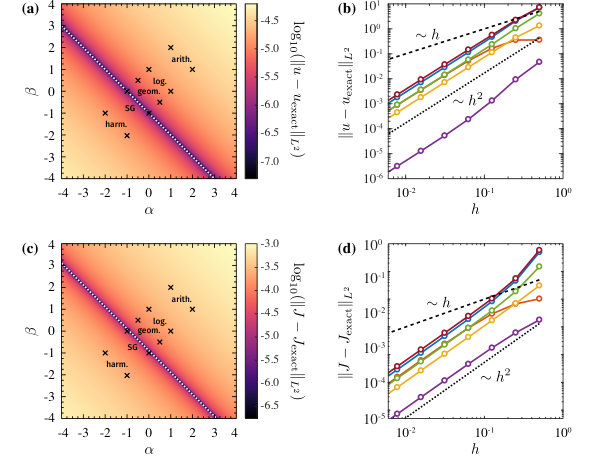
Refer to caption
Figure 2. Discretization errors and convergence behavior of the numerically computed uu and JJ in Example 6.2 using the Stolarsky mean schemes. The errors in (a) and (c) are color-coded. The coloring of the means in (b) and (d) is the same as in Figure 1 (b). The plots clearly show a superior performance of the Scharfetter–Gummel scheme, which corresponds to the Stolarsky mean S0,−1S_{0,-1} for the approximation of both the density uu and the flux JJ.

The numerical results are show in Figure 2. The discretization errors of both the density uu and the flux JJ shown in Figure 2 (a) and (c) exhibit a sharp minimum on α+β=−1\alpha+\beta=-1. This includes the Scharfetter–Gummel mean S0,−1S_{0,-1}, which converges fastest to the exact reference solutions for uu and JJ, as shown in 2 (b) and (d). The SQRA scheme, with geometric mean Sα,−αS_{\alpha,-\alpha}, is found to be second best in the present example.

The numerical results are in line with our previous statements from Remark 5.6: In the case of strong gradients ∇V\nabla V, the Scharfetter–Gummel scheme provides the most accurate flux discretization, in particular, the SG mean S0,−1S_{0,-1} is the only Stolarsky mean that recovers the upwind scheme (1.5). Away from that drift-dominated regime, the situation is less clear and other averages Sα,βS_{\alpha,\beta} can be superior, see for instance Example 6.1.

Appendix A Appendix

A.1. A General Poincaré Inequality

We derive a general Poincaré inequality on meshes. The idea behind the proof seems to go back to Hummel [Hum99] and has been adapted in a series of works e.g. [Hei18, HKP17]. Let e0=0e_{0}=0 and (ei)i=1,…,n(e_{i})_{i=1,\dots,n} be the canonical basis of ℝn\mathbb{R}^{n}. Define:

Dd−1:={ν∈𝕊d−1|∃m∈{1,⋯,d}:ν⋅ei=0∀i∈{0,1,⋯,m−1}andν⋅em>0}.D^{d-1}:=\{\nu\in\mathbb{S}^{d-1}\,\,|\,\,\exists m\in\left\{1,\cdots,d\right\}:\nu\cdot e_{i}=0\,\,\forall\,\,i\in\left\{0,1,\cdots,m-1\right\}\,\,\textnormal{and}\,\,\nu\cdot e_{m}>0\}\,.

Every ν∈𝕊d−1\nu\in\mathbb{S}^{d-1} satisfies ν⋅ei≠0\nu\cdot e_{i}\neq 0 for at least one eie_{i}. Thus, for every ν∈𝕊d−1\nu\in\mathbb{S}^{d-1} it holds ν∈Dd−1\nu\in D^{d-1} if and only if −ν∉Dd−1-\nu\not\in D^{d-1}.

We denote Γ=⋃σ∈ℰΩσ\Gamma=\bigcup_{\sigma\in\mathcal{E}_{\Omega}}\sigma and say that x∈Γx\in\Gamma is a Lipschitz point if Γ\Gamma is a Lipschitz graph in a neighborhood of xx. The set of Lipschitz-Points is called ΓL⊂Γ\Gamma_{L}\subset\Gamma and we note that for the (d−1)\left(d-1\right)-dimensional Hausdorff-measure of Γ\ΓL\Gamma\backslash\Gamma_{L} it holds ℋd−1​(Γ\ΓL)=0\mathcal{H}^{d-1}\left(\Gamma\backslash\Gamma_{L}\right)=0.

For x∈ΓLx\in\Gamma_{L}, we denote νx∈Dd−1\nu_{x}\in D^{d-1} the normal vector to Γ\Gamma in xx.. Let

𝒞01(Ω;Γ):={u∈C(Ω\Γ):u|∂Ω≡0,∀i∃vi∈C1(Ωi¯):u|Ωi=vi}\mathcal{C}_{0}^{1}(\Omega;\Gamma):=\left\{u\in C(\Omega\backslash\Gamma)\,\,:\;\,u|_{\partial\Omega}\equiv 0\,,\;\forall i\,\exists v_{i}\in C^{1}\left(\overline{\Omega_{i}}\right):\,u|_{\Omega_{i}}=v_{i}\right\}

and for u∈𝒞K,01​(Ω)u\in\mathcal{C}_{K,0}^{1}(\Omega) define in Lipschitz points x∈ΓLx\in\Gamma_{L}

u±​(x):=limh→0(u⁡(x±h​νx)),\lsem​u​\rsem​(x):=u+​(x)−u−​(x).u_{\pm}(x):=\lim_{h\to 0}\left(u\left(x\pm h\nu_{x}\right)\right)\,,~~~\lsem u\rsem(x):=u_{+}(x)-u_{-}(x)\,.

For two points x,y∈ℝnx,y\in\mathbb{R}^{n} denote (x,y)(x,y) the closed straight line segment connecting xx and yy and for ξ∈(x,y)∩ΓL\xi\in(x,y)\cap\Gamma_{L} denote

\lsem​u​\rsemx,y​(ξ):=limh→0(u⁡(ξ+h⁡(y−x))−u⁡(ξ−h⁡(y−x)))\lsem u\rsem_{x,y}(\xi):=\lim_{h\to 0}\left(u\left(\xi+h(y-x)\right)-u\left(\xi-h(y-x)\right)\right)

the jump of the function uu at ξ\xi in direction (y−x)(y-x), i.e. \lsem​u​\rsemx,y​(ξ)∈±\lsem​u​\rsem​(ξ)\lsem u\rsem_{x,y}(\xi)\in\pm\lsem u\rsem\left(\xi\right). We can extend \lsem​u​\rsem\lsem u\rsem to Γ\Gamma by \lsem​u​\rsem​(x)=0\lsem u\rsem\left(x\right)=0 for x∈Γ\ΓLx\in\Gamma\backslash\Gamma_{L} and define

‖u‖H1​(Ω,Γ)\displaystyle\left\|u\right\|_{H^{1}\left(\Omega;\Gamma\right)} :=(∫Ω\Γ|∇u|2+∫Γ\lsem​u​\rsem2)12,\displaystyle:=\left(\int_{\Omega\backslash\Gamma}\left|\nabla u\right|^{2}+\int_{\Gamma}\lsem u\rsem^{2}\right)^{\frac{1}{2}}\,,
H01​(Ω,Γ)\displaystyle H_{0}^{1}\left(\Omega;\Gamma\right) :=𝒞01​(Ω,Γ)¯‖⋅‖H1​(Ω,Γ).\displaystyle:=\overline{\mathcal{C}_{0}^{1}\left(\Omega;\Gamma\right)}^{\left\|\cdot\right\|_{H^{1}\left(\Omega;\Gamma\right)}}\,.

Then we find the following result:

Lemma A.1 (Semi-discrete Poincaré inequality).

Let Ω⊂ℝd\Omega\subset\mathbb{R}^{d} be a bounded domain. The space H01​(Ω,Γ)H_{0}^{1}\left(\Omega;\Gamma\right) is linear and closed for every s∈[0,12)s\in[0,\frac{1}{2}) and there exists a positive constant Cs>0C_{s}>0 such that the following holds: Suppose there exists a constant C#>0C_{\#}>0 such that for almost all (x,y)∈Ω2\left(x,y\right)\in\Omega^{2} it holds #⁡((x,y)∩Γ)≤C#\#\left(\left(x,y\right)\cap\Gamma\right)\leq C_{\#}.. Then for every u∈H01​(Ω,Γ)u\in H_{0}^{1}\left(\Omega;\Gamma\right) it holds

(A.1) ‖u‖Hs​(Ω)2≤Cs​(C#​∫Γ\lsem​u​\rsem2+‖∇u‖L2​(Ω\Γ)2).\left\|u\right\|_{H^{s}(\Omega)}^{2}\leq C_{s}\left(C_{\#}\int_{\Gamma}\lsem u\rsem^{2}+\left\|\nabla u\right\|_{L^{2}(\Omega\backslash\Gamma)}^{2}\right)\,.

Furthermore, for every u∈H1​(Ω,Γ)u\in H^{1}\left(\Omega;\Gamma\right) and every 𝛈∈ℝd\boldsymbol{\eta}\in\mathbb{R}^{d} it holds

(A.2) ∫Ω|u⁡(x)−u⁡(x+𝜼)|2​𝑑x≤|𝜼|​(C#​∫Γ\lsem​u​\rsem2+‖∇u‖L2​(Ω\Γ)2).\int_{\Omega}\left|u(x)-u(x+\boldsymbol{\eta})\right|^{2}dx\leq\left|\boldsymbol{\eta}\right|\left(C_{\#}\int_{\Gamma}\lsem u\rsem^{2}+\left\|\nabla u\right\|_{L^{2}(\Omega\backslash\Gamma)}^{2}\right)\,.
Proof.

In what follows, given u∈𝒞01​(Ω,Γ)u\in\mathcal{C}_{0}^{1}(\Omega;\Gamma), we write ∇u^​(x):=∇u​(x)\widehat{\nabla u}(x):=\nabla u(x) if x∈Ω\Γx\in\Omega\backslash\Gamma and ∇u^​(x)=0\widehat{\nabla u}(x)=0 else. For y∈ℝdy\in\mathbb{R}^{d} we denote (x,y)={x+s⁡(y−x):s∈[0,1]}\left(x,y\right)=\left\{x+s\left(y-x\right)\,:\;s\in[0,1]\right\}. Using 2​a​b<a2+b22ab<a^{2}+b^{2}, we infer for u∈𝒞01​(Ω,Γ)u\in\mathcal{C}_{0}^{1}(\Omega;\Gamma) and x,y∈Ω¯\Γx,y\in\overline{\Omega}\backslash\Gamma such that (x,y)∩Γ\left(x,y\right)\cap\Gamma is finite the inequality

|u⁡(x)−u⁡(y)|2\displaystyle\left|u(x)-u(y)\right|^{2} ≤(∑ξ∈(x,y)∩Γ\lsem​u​\rsemx,y​(ξ)+∫01∇u^​(x+s⁡(y−x))⋅(x−y)​𝑑s)2\displaystyle\leq\left(\sum_{\xi\in(x,y)\cap\Gamma}\lsem u\rsem_{x,y}(\xi)+\int_{0}^{1}\widehat{\nabla u}\left(x+s(y-x)\right)\cdot\left(x-y\right)ds\right)^{2}
<|x−y|2​∫01|∇u^​(x+s⁡(y−x))|2​𝑑s+(∑ξ∈(x,y)∩Γ\lsem​u​\rsemx,y​(ξ))2\displaystyle<\left|x-y\right|^{2}\int_{0}^{1}\left|\widehat{\nabla u}\left(x+s(y-x)\right)\right|^{2}ds+\left(\sum_{\xi\in(x,y)\cap\Gamma}\lsem u\rsem_{x,y}(\xi)\right)^{2}

Since \lsem​u​\rsemx,y=\lsem​u​\rsem\lsem u\rsem_{x,y}=\lsem u\rsem we compute

(∑ξ∈(x,y)∩Γ\lsem​u​\rsemx,y​(ξ))2≤#⁡((x,y)∩Γ)​∑ξ∈(x,y)∩Γ\lsem​u​\rsem2​(ξ)\left(\sum_{\xi\in(x,y)\cap\Gamma}\lsem u\rsem_{x,y}(\xi)\right)^{2}\leq\#\left(\left(x,y\right)\cap\Gamma\right)\sum_{\xi\in(x,y)\cap\Gamma}\lsem u\rsem^{2}(\xi)

and obtain

|u⁡(x)−u⁡(y)|2\displaystyle\left|u(x)-u(y)\right|^{2} <|x−y|2​∫01|∇u^​(x+s⁡(y−x))|2​𝑑s\displaystyle<\left|x-y\right|^{2}\int_{0}^{1}\left|\widehat{\nabla u}\left(x+s(y-x)\right)\right|^{2}ds
(A.3) +#((x,y)∩Γ)∑ξ∈(x,y)∩Γ\lsemu\rsem2(ξ).\displaystyle\quad+\#\left(\left(x,y\right)\cap\Gamma\right)\sum_{\xi\in(x,y)\cap\Gamma}\lsem u\rsem^{2}(\xi)\,.

We fix η>0\eta>0 and consider the orthonormal basis (ei)i=1,…,d(e_{i})_{i=1,\dots,d} of ℝd\mathbb{R}^{d}. The determinant of the first fundamental form of Γ\Gamma is bigger than 11 almost everywhere. Hence we can observe that

∫Ω∑ξ∈(x,x+η​e1)∩Γ\lsem​u​\rsem2​(ξ)​𝑑x\displaystyle\int_{\Omega}\sum_{\xi\in(x,x+\eta e_{1})\cap\Gamma}\lsem u\rsem^{2}(\xi)\,\mathrm{d}x =∫ℝ(∫ℝd−1∑ξ∈(x,x+η​e1)∩Γ\lsem​u​\rsem2​(ξ)​d​x2​…​d​xd)​d​x1\displaystyle=\int_{\mathbb{R}}\left(\int_{\mathbb{R}^{d-1}}\sum_{\xi\in(x,x+\eta e_{1})\cap\Gamma}\lsem u\rsem^{2}(\xi)\,\mathrm{d}x_{2}\dots\mathrm{d}x_{d}\right)\mathrm{d}x_{1}
≤∫ℝ∫Γ∩((x1,x1+η)×ℝd−1)\lsem​u​\rsem2​(x)​𝑑σ​d​x1\displaystyle\leq\int_{\mathbb{R}}\int_{\Gamma\cap\left(\left(x_{1},x_{1}+\eta\right)\times\mathbb{R}^{d-1}\right)}\lsem u\rsem^{2}(x)\,\mathrm{d}\sigma\,\mathrm{d}x_{1}
≤η​∫Γ\lsem​u​\rsem2​(x)​𝑑x,\displaystyle\leq\eta\int_{\Gamma}\lsem u\rsem^{2}(x)\,\mathrm{d}x\,,

where we used that the surface elements are bigger than 11. Furthermore, we have

η2​∫01|∇u^​(x+s​η​e1)|2​𝑑s=η​∫0η|∇u^​(x+s​e1)|2​𝑑s.\eta^{2}\int_{0}^{1}\left|\widehat{\nabla u}\left(x+s\eta e_{1}\right)\right|^{2}ds=\eta\int_{0}^{\eta}\left|\widehat{\nabla u}\left(x+se_{1}\right)\right|^{2}ds\,.

Replacing e1e_{1} in the above calculations with any unit vector ee, we obtain from integration of (A.3) with y=x+𝜼y=x+\boldsymbol{\eta}, 𝜼=η​e\boldsymbol{\eta}=\eta e, over Ω\Omega that

∫Ω|u⁡(x)−u⁡(x+𝜼)|2​𝑑x≤|𝜼|​(C#​∫Γ\lsem​u​\rsem2+‖∇u‖L2​(Ω\Γ)2).\int_{\Omega}\left|u(x)-u(x+\boldsymbol{\eta})\right|^{2}dx\leq\left|\boldsymbol{\eta}\right|\left(C_{\#}\int_{\Gamma}\lsem u\rsem^{2}+\left\|\nabla u\right\|_{L^{2}(\Omega\backslash\Gamma)}^{2}\right)\,.

Dividing by |𝜼|\left|\boldsymbol{\eta}\right| and integrating over 𝜼∈ℝd\boldsymbol{\eta}\in\mathbb{R}^{d}, we obtain that for every s∈[0,12)s\in[0,\frac{1}{2}) there exists a positive constant Cs>0C_{s}>0 independent from uu and KK such that

(A.4) ‖u‖Hs​(Ω)2≤Cs​(C#​∫Γ\lsem​u​\rsem2+‖∇u‖L2​(Ω\Γ)2).\left\|u\right\|_{H^{s}(\Omega)}^{2}\leq C_{s}\left(C_{\#}\int_{\Gamma}\lsem u\rsem^{2}+\left\|\nabla u\right\|_{L^{2}(\Omega\backslash\Gamma)}^{2}\right)\,.

Hence, by approximation, the last two estimates hold for all u∈H01​(Ω,Γ)u\in H_{0}^{1}\left(\Omega;\Gamma\right).. ∎

A.2. Physical relevance of the geometric mean

Theorem A.2.

Let Si​j=S∗​(πi,πj)S_{ij}=S_{\ast}\left(\pi_{i},\pi_{j}\right) be a Stolarsky mean and let ψ∗\mathsf{\psi^{*}} be a symmetric strictly convex function with ψ∗​(0)=0\mathsf{\psi^{*}}(0)=0. If ∂π(Si​j​ai​j)=0\partial_{\pi}\left(S_{ij}a_{ij}\right)=0 then Si​j=πi​πjS_{ij}=\sqrt{\pi_{i}\pi_{j}} and ψ∗\mathsf{\psi^{*}} is proportional to 𝖢∗\mathsf{C}^{*}.

Proof of Theorem A.2.

The case Si​j=πi​πjS_{ij}=\sqrt{\pi_{i}\pi_{j}} and ψ∗​(ξ)=cosh⁡ξ−1\mathsf{\psi^{*}}(\xi)=\cosh\xi-1 was explained in detail in [Hei18].

In the general case, symmetry of ψ∗\mathsf{\psi^{*}} in ξi−ξj\xi_{i}-\xi_{j} implies ψ∗​(ξi−ξj)=ψ∗​(|ξi−ξj|)\mathsf{\psi^{*}}\left(\xi_{i}-\xi_{j}\right)=\mathsf{\psi^{*}}\left(\left|\xi_{i}-\xi_{j}\right|\right). We make use of the fact that the original 𝖢∗​(ξ)=cosh⁡ξ−1\mathsf{C^{*}}(\xi)=\cosh\xi-1 is a bijection on [0,∞)[0,\infty) and suppose that hence ψ∗​(ξi−ξj)=θ⁡(𝖢∗​(ξi−ξj))\mathsf{\psi^{*}}\left(\xi_{i}-\xi_{j}\right)=\theta\left(\mathsf{C^{*}}\left(\xi_{i}-\xi_{j}\right)\right). This implies particularly that

0≤x​∂x(θ⁡(𝖢∗​(x)))=x​∂ξθ⁡(𝖢∗​(x))​∂x𝖢∗​(x).0\leq x\,\partial_{x}\left(\theta\left(\mathsf{C^{*}}(x)\right)\right)=x\,\partial_{\xi}\theta\left(\mathsf{C^{*}}(x)\right)\partial_{x}\mathsf{C^{*}}(x)\,.

Furhtermore, the symmetry of ψ∗\mathsf{\psi^{*}} implies by the last inequality that ∂ξθ⁡(𝖢∗​(x))>0\partial_{\xi}\theta\left(\mathsf{C^{*}}(x)\right)>0. Inserting this information in (3.13) and (3.14) we observe that

Si​j(uiπi−ujπj)∂ξθ(𝖢∗(ln(uiπi)−ln(ujπj)))−1sinh(ln(uiπi)−ln(ujπj))−1S_{ij}\left(\frac{u_{i}}{\pi_{i}}-\frac{u_{j}}{\pi_{j}}\right)\partial_{\xi}\theta\left(\mathsf{C^{*}}\left(\ln\left(\frac{u_{i}}{\pi_{i}}\right)-\ln\left(\frac{u_{j}}{\pi_{j}}\right)\right)\right)^{-1}\sinh\left(\ln\left(\frac{u_{i}}{\pi_{i}}\right)-\ln\left(\frac{u_{j}}{\pi_{j}}\right)\right)^{-1}

has to be independent from πi\pi_{i} and πj\pi_{j}. From the above case Si​j=πi​πjS_{ij}=\sqrt{\pi_{i}\pi_{j}}, we know that

πi​πj(uiπi−ujπj)sinh(ln(uiπi)−ln(ujπj))−1\sqrt{\pi_{i}\pi_{j}}\left(\frac{u_{i}}{\pi_{i}}-\frac{u_{j}}{\pi_{j}}\right)\sinh\left(\ln\left(\frac{u_{i}}{\pi_{i}}\right)-\ln\left(\frac{u_{j}}{\pi_{j}}\right)\right)^{-1}

is constant in πi\pi_{i} and πj\pi_{j}. Hence it remains to show that

f⁡(πi,πj):=Si​j​πi​πj−1​∂ξψ​(uiuj​πjπi+ujui​πiπj)−1f\left(\pi_{i},\pi_{j}\right):=S_{ij}\sqrt{\pi_{i}\pi_{j}}^{-1}\partial_{\xi}\psi\left(\frac{u_{i}}{u_{j}}\frac{\pi_{j}}{\pi_{i}}+\frac{u_{j}}{u_{i}}\frac{\pi_{i}}{\pi_{j}}\right)^{-1}

is independent from πi\pi_{i} and πj\pi_{j} if and only if ∂ξψ=const\partial_{\xi}\psi=\mathrm{const} and Si​j=πi​πjS_{ij}=\sqrt{\pi_{i}\pi_{j}}.

Assume first that Si​j​πi​πj−1=constS_{ij}\sqrt{\pi_{i}\pi_{j}}^{-1}=\mathrm{const}. Then for p=πiπjp=\frac{\pi_{i}}{\pi_{j}} we obtain that

∂p(∂ξθ​(uiuj​p−1+ujui​p)−1)=0\partial_{p}\left(\partial_{\xi}\theta\left(\frac{u_{i}}{u_{j}}p^{-1}+\frac{u_{j}}{u_{i}}p\right)^{-1}\right)=0

has to hold. This implies that ∂ξψ=const\partial_{\xi}\psi=\mathrm{const}.

If Si​j​πi​πj−1≠constS_{ij}\sqrt{\pi_{i}\pi_{j}}^{-1}\not=\mathrm{const}, we use the definition of the weighted Stolarsky means given in (3.4) and note that

Si​j:=S⁡(πi,πj)=(β⁡(πiα−πjα)α⁡(πiβ−πjβ))1α−β=πj​(β⁡(pα−1)α⁡(pβ−1))1α−β,S_{ij}:=S\left(\pi_{i},\pi_{j}\right)=\left(\frac{\beta(\pi_{i}^{\alpha}-\pi_{j}^{\alpha})}{\alpha(\pi_{i}^{\beta}-\pi_{j}^{\beta})}\right)^{\frac{1}{\alpha-\beta}}=\pi_{j}\left(\frac{\beta(p^{\alpha}-1)}{\alpha(p^{\beta}-1)}\right)^{\frac{1}{\alpha-\beta}}\,,

where again p=πiπjp=\frac{\pi_{i}}{\pi_{j}}. Hence we obtain that

f⁡(πi,πj)\displaystyle f\left(\pi_{i},\pi_{j}\right) =f~​(p):=1p​(β⁡(pα−1)α⁡(pβ−1))1α−β​∂ξθ​(uiuj​p−1+ujui​p)−1\displaystyle=\tilde{f}(p):=\sqrt{\frac{1}{p}}\left(\frac{\beta(p^{\alpha}-1)}{\alpha(p^{\beta}-1)}\right)^{\frac{1}{\alpha-\beta}}\partial_{\xi}\theta\left(\frac{u_{i}}{u_{j}}p^{-1}+\frac{u_{j}}{u_{i}}p\right)^{-1}
=(β⁡(pα2−p−α2)α⁡(pβ2−p−β2))1α−β​∂ξθ​(uiuj​p−1+ujui​p)−1\displaystyle=\left(\frac{\beta\left(p^{\frac{\alpha}{2}}-p^{-\frac{\alpha}{2}}\right)}{\alpha\left(p^{\frac{\beta}{2}}-p^{-\frac{\beta}{2}}\right)}\right)^{\frac{1}{\alpha-\beta}}\partial_{\xi}\theta\left(\frac{u_{i}}{u_{j}}p^{-1}+\frac{u_{j}}{u_{i}}p\right)^{-1}

has to be independent of πi\pi_{i} and πj\pi_{j}. But then, f~\tilde{f} is independent of pp. Now, we define a=ujuia=\frac{u_{j}}{u_{i}} and observe that

f~​(1a2​p)=(β⁡((a2​p)−α2−(a2​p)α2)α⁡((a2​p)−β2−(a2​p)β2))1α−β​∂ξθ​(uiuj​p−1+ujui​p)−1.\tilde{f}\left(\frac{1}{a^{2}p}\right)=\left(\frac{\beta\left(\left(a^{2}p\right)^{-\frac{\alpha}{2}}-\left(a^{2}p\right)^{\frac{\alpha}{2}}\right)}{\alpha\left(\left(a^{2}p\right)^{-\frac{\beta}{2}}-\left(a^{2}p\right)^{\frac{\beta}{2}}\right)}\right)^{\frac{1}{\alpha-\beta}}\partial_{\xi}\theta\left(\frac{u_{i}}{u_{j}}p^{-1}+\frac{u_{j}}{u_{i}}p\right)^{-1}.

We assume for α≠β\alpha\neq\beta. The case α=β\alpha=\beta can follows by continuity. For any pp it should holds f~​(1a2​p)=f~​(p)\tilde{f}\left(\frac{1}{a^{2}p}\right)=\tilde{f}(p), which implies

(β⁡(pα2−p−α2)α⁡(pβ2−p−β2))1α−β=(β⁡((a2​p)−α2−(a2​p)α2)α⁡((a2​p)−β2−(a2​p)β2))1α−β,\left(\frac{\beta\left(p^{\frac{\alpha}{2}}-p^{-\frac{\alpha}{2}}\right)}{\alpha\left(p^{\frac{\beta}{2}}-p^{-\frac{\beta}{2}}\right)}\right)^{\frac{1}{\alpha-\beta}}=\left(\frac{\beta\left(\left(a^{2}p\right)^{-\frac{\alpha}{2}}-\left(a^{2}p\right)^{\frac{\alpha}{2}}\right)}{\alpha\left(\left(a^{2}p\right)^{-\frac{\beta}{2}}-\left(a^{2}p\right)^{\frac{\beta}{2}}\right)}\right)^{\frac{1}{\alpha-\beta}},

or equivalently, after introducing q2=pq^{2}=p,

(aα−aβ)​qα+β+(aβ−a−α)​qβ−α+(a−β−aα)​qα−β+(a−α−a−β)​q−β−α=0.\left(a^{\alpha}-a^{\beta}\right)q^{\alpha+\beta}+\left(a^{\beta}-a^{-\alpha}\right)q^{\beta-\alpha}+\left(a^{-\beta}-a^{\alpha}\right)q^{\alpha-\beta}+\left(a^{-\alpha}-a^{-\beta}\right)q^{-\beta-\alpha}=0.

Since α≠β\alpha\neq\beta, one of the terms q±α±βq^{\pm\alpha\pm\beta} grows faster than the other. Hence we conclude that aα=a±βa^{\alpha}=a^{\pm\beta} which means, a=1a=1, a contradiction. ∎

A.3. Properties of the Stolarsky mean

Lemma A.3.

For every of the above Stolarsky means S∗​(x,y)S_{\ast}(x,y) it holds

∂xS∗(x,x)=∂yS∗(x,x)=12and∂x2S∗(x,x)=∂y2S∗(x,x)=−∂x​y2S∗(x,x)=−∂y​x2S∗(x,x).\partial_{x}S_{\ast}(x,x)=\partial_{y}S_{\ast}\left(x,x\right)=\frac{1}{2}~~\text{and}~~\partial_{x}^{2}S_{\ast}\left(x,x\right)=\partial_{y}^{2}S_{\ast}\left(x,x\right)=-\partial_{xy}^{2}S_{\ast}\left(x,x\right)=-\partial_{yx}^{2}S_{\ast}\left(x,x\right)\,.
Proof.

Since S∗​(x,x)=xS_{\ast}(x,x)=x and S∗S_{\ast} is symmetric in xx and yy, we find from differentiating ∂xS∗=∂yS∗=12\partial_{x}S_{\ast}=\partial_{y}S_{\ast}=\frac{1}{2}. From the last equality, we find ∂xS∗​(x,x)−∂yS∗​(x,x)=0\partial_{x}S_{\ast}(x,x)-\partial_{y}S_{\ast}(x,x)=0 as well as ∂xS∗​(x,x)+∂yS∗​(x,x)=1\partial_{x}S_{\ast}(x,x)+\partial_{y}S_{\ast}(x,x)=1 and differentiation yields

(A.5) ∂x2S∗​(x,x)−∂y2S∗​(x,x)−∂x​y2S∗​(x,x)+∂y​x2S∗​(x,x)\displaystyle\partial_{x}^{2}S_{\ast}\left(x,x\right)-\partial_{y}^{2}S_{\ast}\left(x,x\right)-\partial_{xy}^{2}S_{\ast}\left(x,x\right)+\partial_{yx}^{2}S_{\ast}\left(x,x\right) =0,\displaystyle=0\,,
(A.6) ∂x2S∗​(x,x)+∂y2S∗​(x,x)+∂x​y2S∗​(x,x)+∂y​x2S∗​(x,x)\displaystyle\partial_{x}^{2}S_{\ast}\left(x,x\right)+\partial_{y}^{2}S_{\ast}\left(x,x\right)+\partial_{xy}^{2}S_{\ast}\left(x,x\right)+\partial_{yx}^{2}S_{\ast}\left(x,x\right) =0.\displaystyle=0\,.

Since −∂x​y2S∗(x,x)+∂y​x2S∗(x,x)=0-\partial_{xy}^{2}S_{\ast}\left(x,x\right)+\partial_{yx}^{2}S_{\ast}\left(x,x\right)=0, equation (A.5) yields ∂x2S∗​(x,x)=∂y2S∗​(x,x)\partial_{x}^{2}S_{\ast}\left(x,x\right)=\partial_{y}^{2}S_{\ast}\left(x,x\right). Inserting the last two relations into (A.6) yields ∂x​y2S∗(x,x)=∂y​x2S∗(x,x)=−∂x2S∗(x,x)\partial_{xy}^{2}S_{\ast}\left(x,x\right)=\partial_{yx}^{2}S_{\ast}\left(x,x\right)=-\partial_{x}^{2}S_{\ast}\left(x,x\right). ∎

Lemma A.4.

It holds (3.5)∂x2Sα,β​(π,π)=112​π​(α+β−3)\partial_{x}^{2}S_{\alpha,\beta}\left(\pi,\pi\right)=\frac{1}{12\pi}\left(\alpha+\beta-3\right).

Proof.

We know from Lemma A.3 that ∂xSα,β​(x,x)=12\partial_{x}S_{\alpha,\beta}\left(x,x\right)=\frac{1}{2} and ∂x2Sα,β(x,x)=−∂y∂xSα,β(x,x)\partial_{x}^{2}S_{\alpha,\beta}\left(x,x\right)=-\partial_{y}\partial_{x}S_{\alpha,\beta}\left(x,x\right). Hence we find

∂xSα,β​(x+h,x−h)−12=(h−h)​(∂x2Sα,β​(x,x)∂y∂xSα,β​(x,x))=2​h​∂x2Sα,β​(x,x).\partial_{x}S_{\alpha,\beta}\left(x+h,x-h\right)-\frac{1}{2}=\left(\begin{array}[]{c}h\\ -h\end{array}\right)\left(\begin{array}[]{c}\partial_{x}^{2}S_{\alpha,\beta}\left(x,x\right)\\ \partial_{y}\partial_{x}S_{\alpha,\beta}\left(x,x\right)\end{array}\right)=2h\partial_{x}^{2}S_{\alpha,\beta}\left(x,x\right)\,.

We make use of the explicit form

∂xSα,β​(x,y)=(βα)1α−β​(xα−yα)1α−β−1(xβ−yβ)1α−β−1​α⁡(xβ−yβ)​xα−β⁡(xα−yα)​xβ(α−β)​x​(xβ−yβ)2\partial_{x}S_{\alpha,\beta}\left(x,y\right)=\left(\frac{\beta}{\alpha}\right)^{\frac{1}{\alpha-\beta}}\frac{\left(x^{\alpha}-y^{\alpha}\right)^{\frac{1}{\alpha-\beta}-1}}{\left(x^{\beta}-y^{\beta}\right)^{\frac{1}{\alpha-\beta}-1}}\frac{\alpha\left(x^{\beta}-y^{\beta}\right)x^{\alpha}-\beta\left(x^{\alpha}-y^{\alpha}\right)x^{\beta}}{\left(\alpha-\beta\right)\,\,x\,\,\left(x^{\beta}-y^{\beta}\right)^{2}}

for x≠yx\not=y. We insert x=x+hx=x+h and y=x−hy=x-h and make use of the following expansions

((x+h)α−(x−h)α)c\displaystyle\left(\left(x+h\right)^{\alpha}-\left(x-h\right)^{\alpha}\right)^{c} =(α​h​xα−1)c​(2c+O⁡(h2))\displaystyle=\left(\alpha hx^{\alpha-1}\right)^{c}\left(2^{c}+O\left(h^{2}\right)\right)
β⁡((x+h)α−(x−h)α)​(x+h)β\displaystyle\beta\left(\left(x+h\right)^{\alpha}-\left(x-h\right)^{\alpha}\right)\left(x+h\right)^{\beta} =2​α​β​h​xα+β−1+2​α​β2​h2​xα+β−2\displaystyle=2\alpha\beta hx^{\alpha+\beta-1}+2\alpha\beta^{2}h^{2}x^{\alpha+\beta-2}
+13​α​β​h3​(α2−3​α+3​β2−3​β+2)+O⁡(h4)\displaystyle+\frac{1}{3}\alpha\beta h^{3}\left(\alpha^{2}-3\alpha+3\beta^{2}-3\beta+2\right)+O\left(h^{4}\right)
α⁡((x+h)β−(x−h)β)​(x+h)α\displaystyle\alpha\left(\left(x+h\right)^{\beta}-\left(x-h\right)^{\beta}\right)\left(x+h\right)^{\alpha} =2​α​β​h​xα+β−1+2​α2​β​h2​xα+β−2\displaystyle=2\alpha\beta hx^{\alpha+\beta-1}+2\alpha^{2}\beta h^{2}x^{\alpha+\beta-2}
+13​α​β​h3​(β2−3​β+3​α2−3​α+2)+O⁡(h4)\displaystyle+\frac{1}{3}\alpha\beta h^{3}\left(\beta^{2}-3\beta+3\alpha^{2}-3\alpha+2\right)+O\left(h^{4}\right)
(x+h)​((x+h)β−(x−h)β)2\displaystyle\left(x+h\right)\,\left(\left(x+h\right)^{\beta}-\left(x-h\right)^{\beta}\right)^{2} =4​β2​h2​x2​β−1+4​β2​h3​x2​β−2+O⁡(h4)\displaystyle=4\beta^{2}h^{2}x^{2\beta-1}+4\beta^{2}h^{3}x^{2\beta-2}+O\left(h^{4}\right)
α⁡((x+h)β−(x−h)β)​(x+h)α−β⁡((x+h)α−(x−h)α)​(x+h)β=2​α​β​(α−β)​h2​xα+β−2+α​β3​h3​xα+β−3​(2​α2−2​β2)+O⁡(h4)\alpha\left(\left(x+h\right)^{\beta}-\left(x-h\right)^{\beta}\right)\left(x+h\right)^{\alpha}-\beta\left(\left(x+h\right)^{\alpha}-\left(x-h\right)^{\alpha}\right)\left(x+h\right)^{\beta}\\ =2\alpha\beta\left(\alpha-\beta\right)h^{2}x^{\alpha+\beta-2}+\frac{\alpha\beta}{3}h^{3}x^{\alpha+\beta-3}\left(2\alpha^{2}-2\beta^{2}\right)+O\left(h^{4}\right)

to obtain

β⁡(xα−yα)​xβ−α⁡(xβ−yβ)​xα(α−β)​x​(xβ−yβ)2\displaystyle\frac{\beta\left(x^{\alpha}-y^{\alpha}\right)x^{\beta}-\alpha\left(x^{\beta}-y^{\beta}\right)x^{\alpha}}{\left(\alpha-\beta\right)\,\,x\,\,\left(x^{\beta}-y^{\beta}\right)^{2}} =α⁡(xα+β−2+h​13​xα+β−3​(α+β)+O⁡(h2))2​β​(x2​β−1+h​x2​β−2+O⁡(h2))\displaystyle=\frac{\alpha\left(x^{\alpha+\beta-2}+h\frac{1}{3}x^{\alpha+\beta-3}\left(\alpha+\beta\right)+O\left(h^{2}\right)\right)}{2\beta\left(x^{2\beta-1}+hx^{2\beta-2}+O\left(h^{2}\right)\right)}

and

(xα−yα)1α−β−1(xβ−yβ)1α−β−1≈(αβ)1α−β−1​(xα−1​(1+O⁡(h2))xβ−1​(1+O⁡(h2)))1α−β−1.\frac{\left(x^{\alpha}-y^{\alpha}\right)^{\frac{1}{\alpha-\beta}-1}}{\left(x^{\beta}-y^{\beta}\right)^{\frac{1}{\alpha-\beta}-1}}\approx\left(\frac{\alpha}{\beta}\right)^{\frac{1}{\alpha-\beta}-1}\left(\frac{x^{\alpha-1}\left(1+O\left(h^{2}\right)\right)}{x^{\beta-1}\left(1+O\left(h^{2}\right)\right)}\right)^{\frac{1}{\alpha-\beta}-1}\,.

Together with

a+b​hc+d​h\displaystyle\frac{a+bh}{c+dh} =ac+b​c−a​dc2​h+O⁡(h2)\displaystyle=\frac{a}{c}+\frac{bc-ad}{c^{2}}h+O\left(h^{2}\right)
(1+a​h21+b​h2)c\displaystyle\left(\frac{1+ah^{2}}{1+bh^{2}}\right)^{c} =1+c​h2​(a−b)+O⁡(h4)\displaystyle=1+ch^{2}(a-b)+O\left(h^{4}\right)

we find

∂xSα,β​(x+h,x−h)\displaystyle\partial_{x}S_{\alpha,\beta}\left(x+h,x-h\right) =((1+O⁡(h2))(1+O⁡(h2)))1α−β−1​((1+h​13​x−1​(α+β)+O⁡(h2))2​(1+h​x−1+O⁡(h2)))\displaystyle=\left(\frac{\left(1+O\left(h^{2}\right)\right)}{\left(1+O\left(h^{2}\right)\right)}\right)^{\frac{1}{\alpha-\beta}-1}\left(\frac{\left(1+h\frac{1}{3}x^{-1}\left(\alpha+\beta\right)+O\left(h^{2}\right)\right)}{2\left(1+hx^{-1}+O\left(h^{2}\right)\right)}\right)
=(12+23​(α+β)−24​x​h)+O⁡(h2)\displaystyle=\left(\frac{1}{2}+\frac{\frac{2}{3}\left(\alpha+\beta\right)-2}{4\,x}\,h\right)+O\left(h^{2}\right)

and hence (3.5). ∎

A.4. Approximation of potentials to get the SQRA mean

The aim of this section is to provide a class of potentials which are easy to handle and which generate the SQRA-mean S−1,1​(π0,πh)S_{-1,1}(\pi_{0},\pi_{h}) by πmean=(1h​∫0hπ−1)−1\pi_{\mathrm{mean}}=\left(\frac{1}{h}\int_{0}^{h}\pi^{-1}\right)^{-1}. Clearly, choosing the constant potential V⁡(x):=Vc:=−log⁡S−1,1​(π0,πh)V(x):=V_{c}:=-\log S_{-1,1}(\pi_{0},\pi_{h}) we obtain right mean. Although this works for any means, this has two drawbacks

  1. (1)

    The potential jumps and hence the gradient is somewhere infinite, which means that at these points the force on the particles is infinitely high which is not physical.

  2. (2)

    Approximating a general function by piecewise constants, on each interval the accuracy is only of order hh. However, approximating a function by affine interpolation the accuracy is of order h2h^{2} on each interval (see below for the calculation).

So we want to get a potential which may be used as a good approximation (i.e. approximating of order h2h^{2}), is physical (i.e. continuous) and generates the SQRA-mean. Note, that most considerations below also work for other Stolarsky means. For simplicity we focus on the SQRA mean S−1,1S_{-1,1}.

A.4.1. Approximation order for linear approximation

Let us first realize that a linear interpolation provides an approximation of order h2h^{2}. Let V:[0,h]→ℝV:[0,h]\rightarrow\mathbb{R} be a general C2C^{2}-potential. We define with V⁡(0)=V0V(0)=V_{0} and V⁡(h)=VhV(h)=V_{h}

V~​(x)=V0+Vh−V0h​x.\tilde{V}(x)=V_{0}+\frac{V_{h}-V_{0}}{h}x.

Then one easily checks that

V⁡(x)=V0+∂xV⁡(0)​x+12​∂x2V⁡(0)​x2+O⁡(h3)V(x)=V_{0}+\partial_{x}V(0)x+\frac{1}{2}\partial_{x}^{2}V(0)x^{2}+O(h^{3})

and hence,

V⁡(x)−V~​(x)=(∂xV⁡(0)−Vh−V0h)​x+12​∂x2V⁡(0)​x2+O⁡(h3).V(x)-\tilde{V}(x)=\left(\partial_{x}V(0)-\frac{V_{h}-V_{0}}{h}\right)x+\frac{1}{2}\partial_{x}^{2}V(0)x^{2}+O(h^{3}).

Clearly, we also have

Vh=V0+∂xV⁡(0)​h+12​∂x2V⁡(0)​h2+O⁡(h3)V_{h}=V_{0}+\partial_{x}V(0)h+\frac{1}{2}\partial_{x}^{2}V(0)h^{2}+O(h^{3})

which yields

V(x)−V~(x)=−12∂x2V(0)hx+12∂x2V(0)x2+O(h3)=12∂x2V(0)(x−h)x+O(h3)=O(h2).V(x)-\tilde{V}(x)=-\frac{1}{2}\partial_{x}^{2}V(0)hx+\frac{1}{2}\partial_{x}^{2}V(0)x^{2}+O(h^{3})=\frac{1}{2}\partial_{x}^{2}V(0)(x-h)x+O(h^{3})=O(h^{2}).

A.4.2. Definition of potentials V^\hat{V} which generate the SQRA mean

We consider a piecewise linear potential of the form

V^​(x)={Vc−V0x1​x+V0,x∈[0,x1]Vc,x∈[x1,x2]Vh−Vch−x2​(x−x2)+Vc,x∈[x2,h].\hat{V}(x)=\begin{cases}\frac{V_{c}-V_{0}}{x_{1}}x+V_{0}&,x\in[0,x_{1}]\\ V_{c}&,x\in[x_{1},x_{2}]\\ \frac{V_{h}-V_{c}}{h-x_{2}}(x-x_{2})+V_{c}&,x\in[x_{2},h]\end{cases}.

where x1,x2∈[0,h]x_{1},x_{2}\in[0,h] are firstly arbitrary and Vc=−log⁡S−1,1​(π0,πh)=12​(Vh+V0)V_{c}=-\log S_{-1,1}(\pi_{0},\pi_{h})=\tfrac{1}{2}(V_{h}+V_{0}) . The potential is clearly continuous. Then

1h​∫0heOPENV⁡(CLOSE^​x)​𝑑x=x1h​eVc−eV0Vc−V0+x2−x1h​eVc+h−x2h​eVh−eVcVh−Vc.\frac{1}{h}\int_{0}^{h}\mathrm{{e}}^{\hat{V(}x)}\mathrm{d}x=\frac{x_{1}}{h}\frac{\mathrm{{e}}^{V_{c}}-\mathrm{{e}}^{V_{0}}}{V_{c}-V_{0}}+\frac{x_{2}-x_{1}}{h}\mathrm{{e}}^{V_{c}}+\frac{h-x_{2}}{h}\frac{\mathrm{{e}}^{V_{h}}-\mathrm{{e}}^{V_{c}}}{V_{h}-V_{c}}.

Introducing the ratios α=x1h\alpha=\frac{x_{1}}{h} and β=h−x2h\beta=\frac{h-x_{2}}{h} (which are in [0,1/2][0,1/2]) , we want to solve 1h​∫0heV^​(x)​𝑑x=e12​(Vh+V0)\frac{1}{h}\int_{0}^{h}\mathrm{{e}}^{\hat{V}(x)}\mathrm{d}x=\mathrm{{e}}^{\tfrac{1}{2}(V_{h}+V_{0})}. Indeed, introducing the difference of the potentials V¯=Vh−V0\bar{V}=V_{h}-V_{0}, we obtain

λ=αβ=eV¯/2−V¯/2−1e−V¯/2+V¯/2−1≈1+13​V¯+118​V¯2.\lambda=\frac{\alpha}{\beta}=\frac{\mathrm{{e}}^{\bar{V}/2}-\bar{V}/2-1}{\mathrm{{e}}^{-\bar{V}/2}+\bar{V}/2-1}\approx 1+\frac{1}{3}\bar{V}+\frac{1}{18}\bar{V}^{2}.

Hence, any value α,β\alpha,\beta satisfying this ratio generates a potential with the SQRA-mean.

A.4.3. Proof that the potential approximates an arbitrary potential of order h2h^{2}

Since the linear potentials approximates a general potential of order h2h^{2} it suffices to approximate the linear potential V~\tilde{V} by V^\hat{V}. We show that there are α,β\alpha,\beta satisfying αβ=λ\frac{\alpha}{\beta}=\lambda, such that ‖V^−V~‖C⁡([xi,xi+1])=O⁡(h2)\|\hat{V}-\tilde{V}\|_{C([x_{i},x_{i+1}])}=O(h^{2}). The difference of V^\hat{V} and V~\tilde{V} is the largest at x=x1x=x_{1} or x=x2x=x_{2}. We estimate both differences. We have

V~​(x1)=V0+Vh−V0h​x1=V0+α​V¯,V~​(x2)=V0+Vh−V0h​x2=V0+(1−β)​V¯.\tilde{V}(x_{1})=V_{0}+\frac{V_{h}-V_{0}}{h}x_{1}=V_{0}+\alpha\bar{V},\ \ \tilde{V}(x_{2})=V_{0}+\frac{V_{h}-V_{0}}{h}x_{2}=V_{0}+(1-\beta)\bar{V}.

Hence we have to estimate

Δ1:=|V0−Vc+α​V¯|,Δ2:=|V0−Vc+(1−β)​V¯|.\Delta_{1}:=|V_{0}-V_{c}+\alpha\bar{V}|,\ \ \Delta_{2}:=|V_{0}-V_{c}+(1-\beta)\bar{V}|.

In the case of SQRA, one possible choice for α,β\alpha,\beta is given by α+β=1\alpha+\beta=1. Then Δ1=Δ2=|V0−Vc+α​V¯|=|V0−Vc+λ1+λ​V¯|=11+λ​|(1+λ)​(V0−Vc)+λ​V¯|\Delta_{1}=\Delta_{2}=|V_{0}-V_{c}+\alpha\bar{V}|=|V_{0}-V_{c}+\frac{\lambda}{1+\lambda}\bar{V}|=\frac{1}{1+\lambda}|(1+\lambda)(V_{0}-V_{c})+\lambda\bar{V}|. We have V0−Vc=−V¯/2V_{0}-V_{c}=-\bar{V}/2, and hence

Δ1=Δ2=11+λ​V¯2​|λ−1|.\Delta_{1}=\Delta_{2}=\frac{1}{1+\lambda}\frac{\bar{V}}{2}|\lambda-1|.

One can check that λ≈1+V¯/3\lambda\approx 1+\bar{V}/3 and hence, Δ1+Δ2≈V26≈O⁡(h2)\Delta_{1}+\Delta_{2}\approx\frac{V^{2}}{6}\approx O(h^{2}).

References

  • [AS55] D. N. de G. Allan and R. V. Southwell. Relaxation methods applied to determine the motion in two dimensions of a viscous fluid past a fixed cylinder. Q. J. Mech. Appl. Math., 8(2):129–145, 1955.
  • [BMP89] Franco Brezzi, Luisa Donatella Marini, and Paola Pietra. Numerical simulation of semiconductor devices. Comput. Methods Appl. Mech. Eng., 75(1-3):493–514, 1989.
  • [Bre71] Richard P. Brent. An algorithm with guaranteed convergence for finding a zero of a function. Comput. J., 14(4):422–425, 1971.
  • [CHLZ12] Shui-Nee Chow, Wen Huang, Yao Li, and Haomin Zhou. Fokker-Planck equations for a free energy functional or Markov process on a graph. 203(3):969–1008, 2012.
  • [DFM18] Patrick Dondl, Thomas Frenzel, and Alexander Mielke. A gradient system with a wiggly energy and relaxed EDP-convergence. ESAIM Control Optim. Calc. Var., 2018. To appear. WIAS preprint 2459.
  • [DHWK] L. Donati, M. Heida, M. Weber, and B. Keller. Estimation of the initesimal generator by square-root approximation. In preparation.
  • [DJSD15] Purushottam D Dixit, Abhinav Jain, Gerhard Stock, and Ken A Dill. Inferring transition rates of networks from populations in continuous-time markov processes. Journal of chemical theory and computation, 11(11):5464–5472, 2015.
  • [DL15] Karoline Disser and Matthias Liero. On gradient structures for Markov chains and the passage to Wasserstein gradient flows. Networks Heterg. Media, 10(2):233–253, 2015.
  • [DPD18] Daniele A Di Pietro and Jérôme Droniou. A third strang lemma and an aubin–nitsche trick for schemes in fully discrete formulation. Calcolo, 55(3):40, 2018.
  • [EFG06] R. Eymard, J. Fuhrmann, and K. Gärtner. A finite volume scheme for nonlinear parabolic equations derived from one-dimensional local dirichlet problems. Numer. Math., 102(3):463–495, 2006.
  • [EM12] Matthias Erbar and Jan Maas. Ricci curvature of finite Markov chains via convexity of the entropy. 206(3):997–1038, 2012.
  • [Eva98] L.C. Evans. Partial Differential Equations. AMS, 1998.
  • [FKF17] Patricio Farrell, Thomas Koprucki, and Jürgen Fuhrmann. Computational and analytical comparison of flux discretizations for the semiconductor device equations beyond Boltzmann statistics. Journal of Computational Physics, 346:497–513, 2017.
  • [FKN+19] Konstantin Fackeldey, Péter Koltai, Peter Névir, Henning Rust, Axel Schild, and Marcus Weber. From metastable to coherent sets – time-discretization schemes. Chaos: An Interdisciplinary Journal of Nonlinear Science, 29(1):012101, 2019.
  • [FL19] Thomas Frenzel and Matthias Liero. Effective diffusion in thin structures via generalized gradient systems and EDP-convergence. WIAS Preprint 2601, 2019.
  • [FRD+17] Patricio Farrell, Nella Rotundo, Duy Hai Doan, Markus Kantner, Jürgen Fuhrmann, and Thomas Koprucki. Drift-Diffusion Models. In Joachim Piprek, editor, Handbook of Optoelectronic Device Modeling and Simulation: Lasers, Modulators, Photodetectors, Solar Cells, and Numerical Methods, volume 2, chapter 50, pages 731–771. CRC Press, Taylor & Francis Group, Boca Raton, 2017.
  • [GHV00] Thierry Gallouët, Raphaele Herbin, and Marie Hélene Vignal. Error estimates on the approximate finite volume solution of convection diffusion equations with general boundary conditions. SIAM Journal on Numerical Analysis, 37(6):1935–1972, 2000.
  • [GKMP19] Peter Gladbach, Eva Kopfer, Jan Maas, and Lorenzo Portinale. Homogenisation of one-dimensional discrete optimal transport. arXiv:1905.05757, 2019.
  • [Hei18] Martin Heida. Convergences of the squareroot approximation scheme to the Fokker–Planck operator. Mathematical Models and Methods in Applied Sciences, 28(13):2599–2635, 2018.
  • [HKP17] Martin Heida, Ralf Kornhuber, and Joscha Podlesny. Fractal homogenization of multiscale interface problems. arXiv preprint arXiv:1712.01172, 2017.
  • [HMR11] M. Heida, J. Màlek, and K.R. Rajagopal. On the development and generalizations of Allen-Cahn and Stefan equations within a thermodynmic framework. to be submitted to Zeitschrift für Angewandte Mathematik und Physik (ZAMP), 2011.
  • [Hum99] H.K. Hummel. Homogenization of Periodic and Random Multidimensional Microstructures. PhD thesis, Technische Universität Bergakademie Freiberg, 1999.
  • [Il’69] A. M. Il’in. Differencing scheme for a differential equation with a small parameter affecting the highest derivative. Mathematical notes of the Academy of Sciences of the USSR, 6(2):237–248, 1969. Translated from Mat. Zametki, Vol. 6, No. 2, pp. 237–248 (1969).
  • [JKO98] Richard Jordan, David Kinderlehrer, and Felix Otto. The variational formulation of the fokker–planck equation. SIAM journal on mathematical analysis, 29(1):1–17, 1998.
  • [Kan20] Markus Kantner. Generalized Scharfetter–Gummel schemes for electro-thermal transport in degenerate semiconductors using the Kelvin formula for the Seebeck coefficient. Journal of Computational Physics, 402:109091, 2020.
  • [LFW13] Han Cheng Lie, Konstantin Fackeldey, and Marcus Weber. A square root approximation of transition rates for a markov state model. SIAM Journal on Matrix Analysis and Applications, 34:738–756, 2013.
  • [LMPR17] Matthias Liero, Alexander Mielke, Mark A. Peletier, and D. R. Michiel Renger. On microscopic origins of generalized gradient structures. Discr. Cont. Dynam. Systems Ser. S, 10(1):1–35, 2017.
  • [Maa11] Jan Maas. Gradient flows of the entropy for finite Markov chains. J. Funct. Anal., 261:2250–2292, 2011.
  • [Mar15] René Marcelin. Contribution a l’étude de la cinétique physico-chimique. Annales de Physique, III:120–231, 1915.
  • [Mar86] P. A. Markowich. The stationary Semiconductor device equations. Springer, Vienna, 1986.
  • [Mie11] Alexander Mielke. A gradient structure for reaction-diffusion systems and for energy-drift-diffusion systems. Nonlinearity, 24:1329–1346, 2011.
  • [Mie13a] Alexander Mielke. Geodesic convexity of the relative entropy in reversible markov chains. Calculus of Variations and Partial Differential Equations, 48(1):1–31, 2013.
  • [Mie13b] Alexander Mielke. Geodesic convexity of the relative entropy in reversible Markov chains. Calc. Var. Part. Diff. Eqns., 48(1):1–31, 2013.
  • [Mie16] Alexander Mielke. On evolutionary Γ\Gamma-convergence for gradient systems (Ch. 3). In A. Muntean, J. Rademacher, and A. Zagaris, editors, Macroscopic and Large Scale Phenomena: Coarse Graining, Mean Field Limits and Ergodicity, Lecture Notes in Applied Math. Mechanics Vol. 3, pages 187–249. Springer, 2016. Proc. of Summer School in Twente University, June 2012.
  • [MPPR17] Alexander Mielke, Robert I. A. Patterson, Mark A. Peletier, and D. R. Michiel Renger. Non-equilibrium thermodynamical principles for chemical reactions with mass-action kinetics. SIAM J. Appl. Math., 77(4):1562–1585, 2017.
  • [MPR14] Alexander Mielke, Mark A. Peletier, and D. R. Michiel Renger. On the relation between gradient flows and the large-deviation principle, with applications to Markov chains and diffusion. Potential Analysis, 41(4):1293–1327, 2014.
  • [MS19] Alexander Mielke and Artur Stephan. Coarse-graining via edp-convergence for linear fast-slow reaction systems. WIAS preprint 2643, 2019.
  • [MW94] J J H Miller and Song Wang. An analysis of the Scharfetter–Gummel box method for the stationary semiconductor device equations. ESAIM: Mathematical Modelling and Numerical Analysis, 28(2):123–140, 1994.
  • [SG69] D.L. Scharfetter and H.K. Gummel. Large-signal analysis of a silicon read diode oscillator. IEEE Trans. Electron Devices, 16(1):64–77, 1969.
  • [Sto75] Kenneth B. Stolarsky. Generalizations of the logarithmic mean. Mathematics Magazine, 48(2):87–92, 1975.
  • [vR50] W. W. van Roosbroeck. Theory of the flow of electrons and holes in germanium and other semiconductors. Bell Syst. Tech. J., 29(4):560–607, Oct 1950.
  • [WE17] Marcus Weber and Natalia Ernst. A fuzzy-set theoretical framework for computing exit rates of rare events in potential-driven diffusion processes. arXiv preprint arXiv:1708.00679, 2017.
  • [WR17] Inc. Wolfram Research. Mathematica, 2017.