Efficient model-based Bioequivalence Testing

We consider the following sub-hypotheses of $H_{0}$ as described in (2.1) given by

$\displaystyle H_{0,-\delta}:\mu_{T}-\mu_{R}\leq-\delta\text{ and }H_{0,\delta}:\mu_{T}-\mu_{R}\geq\delta.$

(2.3)

The idea of the TOST consists in testing each of these hypotheses separately by a one-sided test. The global null hypothesis $H_{0}$ in (2.1) is rejected with a type I error $\alpha$ if both one-sided hypotheses are rejected with a type I error $\alpha$. To be precise let $X_{T,1},\ldots X_{T,N_{T}}$ and $X_{R,1},\ldots X_{R,N_{R}}$ denote the samples from the test (T) and a reference product (R) respectively and denote by $\bar{X}_{k}=\tfrac{1}{N_{k}}\sum_{i=1}^{N_{k}}X_{k,i}$ ($k=R,T$) the mean measured endpoints (over all individuals for the two treatments). Under the assumption that the random variables $\{X_{k,i}~:~i=1,\ldots N_{k},~k=R,T\}$ are independent and normally distributed with a common (but unknown) variance $\sigma^{2}$, that is $X_{R,i}\sim{\cal N}(\mu_{R},\sigma^{2})$; $i=1\ldots,N_{R}$ ,  $X_{T,i}\sim{\cal N}(\mu_{T},\sigma^{2})$; $i=1\ldots,N_{T}$ we have for the corresponding means

$$\bar{X}_{R}\sim\mathcal{N}(\mu_{R},\tfrac{\sigma^{2}}{N_{R}})\text{ and }\bar{X}_{T}\sim\mathcal{N}(\mu_{T},\tfrac{\sigma^{2}}{N_{T}}).$$

(2.4)

In applications $X_{R,i}$ and $X_{T,i}$ usually represent $AUC_{k}$ and $C_{max_{k}}$, $k=R,T$, which are typically assumed to be lognormally distributed (see Lacey et al., 1997). We denote by $\sigma_{P}^{2}:=\big(\tfrac{1}{N_{R}}+\tfrac{1}{N_{T}}\big)\sigma^{2}$ the pooled variance and by $d:=\mu_{T}-\mu_{R}$ the difference between the expectations of the reference and the treatment group. This yields for the difference of the means

$$\bar{X}_{T}-\bar{X}_{R}\sim\mathcal{N}(d,\sigma_{P}^{2}).$$

(2.5)

The unknown variance $\sigma_{P}^{2}$ is estimated by

$$\hat{\sigma}_{P}^{2}:=\big(\tfrac{1}{N_{T}}+\tfrac{1}{N_{R}}\big)\hat{\sigma}^{2},$$

(2.6)

where

$$\hat{\sigma}^{2}=\frac{1}{N_{T}+N_{R}-2}\sum_{k\in\{R,T\}}\sum_{i=1}^{N_{k}}\left(X_{k,i}-\bar{X}_{k}\right)^{2}.$$

Consequently the null hypothesis in (2.1) is rejected if

$$\frac{\bar{X}_{T}-\bar{X}_{R}-(-\delta)}{\hat{\sigma}_{P}}\geq t_{N-2,1-\alpha}\text{ and }\frac{\bar{X}_{T}-\bar{X}_{R}-\delta}{\hat{\sigma}_{P}}\leq-t_{N-2,1-\alpha},$$

(2.7)

where $t_{N,1-\alpha}$ is the $(1-\alpha)$-quantile of the $t$-distribution with $N-2=N_{R}+N_{T}-2$ degrees of freedom (see for example Chow and Liu, 1992). This method is equivalent to constructing a $(1-2\alpha)$-confidence interval for $\mu_{T}-\mu_{R}$ and concluding bioequivalence if its completely contained in the equivalence interval $\left[-\delta,\delta\right]$ (see Schuirmann, 1987).

The approach presented above has been extended for model-based bioequivalence inference by Dubois et al., 2011 and will be explained in detail in Section 3.2.

In this section we will review an alternative test which is (asymptotically) the most powerful test in this setting. In the case of known variances this property is well known in the literature on mathematical statistics (see, for example, Romano et al., 2005), and, for the sake of completeness, a proof of optimality will be given in the Appendix A.2, where we also review some aspects of the power of the TOST. These considerations motivate the model-based method, which we will propose in the following Section 3.3.

To be precise, let $\mathcal{N}_{F}(d,\sigma_{P}^{2})$ denote the folded normal distribution with parameters $(d,\sigma_{P}^{2})$, that is the distribution of the random variable $|Z|$, where $Z\sim\mathcal{N}(d,\sigma_{P}^{2})$. Due to (2.5) we have for the absolute difference

$$\left|\bar{X}_{T}-\bar{X}_{R}\right|\sim\mathcal{N}_{F}(d,\sigma_{P}^{2}).$$

This result motivates the choice of the quantile determining the decision rule of the test, which is described in the following algorithm.

The quantile $\hat{u}_{\alpha}$ can be calculated solving the equation

$$\alpha=\Phi\left(\tfrac{1}{\hat{\sigma}_{P}}(u-\delta)\right)-\Phi\left(\tfrac{1}{\hat{\sigma}_{P}}(-u-\delta)\right).$$

Alternatively, it can directly be obtained by using statistical software, as for example the $VGAM$ package by Yee, 2015 in R.
The approach presented in Algorithm 2.1 is extended in Algorithm 3.1 for model-based bioequivalence inference, where we will estimate the parameters of interest $\hat{\mu}_{R}$ and $\hat{\mu}_{T}$ by fitting a nonlinear mixed model to the data.

If we are testing for PK bioequivalence considering the hypotheses in (2) we need to calculate estimates of $AUC$ and $C_{\max}$ directly from the data. In this regard the classical approach is given by NCA, as described for example in Gabrielsson and Weiner, 2001. More precisely, $C_{\max}$ is directly obtained from the data, whereas $AUC$ is approximated by the linear trapezoidal rule. This means that the total area under the curve is obtained by separating it into several smaller trapezoids and summing up these areas. Of course the accuracy of this approach strongly depends on the number of measurements as this gives the number of trapezoids but it does not require a model assumption and is widely applicable. As these methods do not take the profile of the blood concentration-time curve into account, we call them NCA-based methods throughout this paper and they will be discussed in more detail in Section 3.

We first consider crossover trials with $K$ periods and $N$ subjects, investigating the difference between a test and a reference treatment. A classical situation is given by the (balanced) two-period, two-sequence crossover design ($K=2$), where the $N/2$ patients receive treatment $R$ in the first period and treatment $T$ in the second one while the other $N/2$ patients receive the treatments in the reverse order.
For each subject concentrations of the drug are measured in all periods and at different sampling points. In order to represent the dependence of the concentration on time for one subject we follow Dubois et al., 2011 and use a non-linear function, say $f$ in order to fit one global model to the data, that is

$$y_{i,j,k}=f(t_{i,j,k},\psi_{i,k})+g(t_{i,j,k},\psi_{i,k})\varepsilon_{i,j,k},$$

(4.1)

where $y_{i,j,k}$ denotes the concentration of the $i$-th subject ($i=1,\ldots N$) at sampling time $t_{i,j,k}$ ($j=1,\ldots,n_{i,k}$) of period $k$ ($k=1,\ldots K$). In (4.1) the residual errors $\varepsilon_{i,j,k}$ are independent and standard-normally distributed random variables and the function $g$ is used to model heteroscedasticity. In particular we consider a combined error model with

$\displaystyle g(t_{i,j,k},\psi_{i,k})=a+b\cdot f(t_{i,j,k},\psi_{i,k}),$

(4.2)

where the parameters $a,b\in\mathbb{R}_{\geq 0}$ account for the additive and the proportional part of the error respectively. This gives for the variance of the errors in (4.1)

$$\mbox{Var}(y_{i,j,k})=(g(t_{i,j,k},\psi_{i,k}))^{2}=|a+b\cdot f(t_{i,j,k},\psi_{i,k})|^{2}.$$

The individual parameters $\psi_{i,k}=(\psi_{i,k,1},\ldots,\psi_{i,k,p})^{\top}$ (of length $p$) are defined by

$$\log(\psi_{i,k,l})=\log{\lambda_{l}}+\beta^{T}_{l}Tr_{i,k}+\beta^{P}_{l}P_{k}+\beta^{S}_{l}S_{i}+\eta_{i,l}+\kappa_{i,k,l},\ l=1,\ldots,p,$$

(4.3)

where $\lambda=(\lambda_{1},\ldots,\lambda_{p})^{\top}$ denotes a vector of fixed effects, $Tr_{i,k}$, $P_{k}$ and $S_{i}$ the (known) vectors of treatment, period and sequence covariates respectively and $\beta^{T}$, $\beta^{P}$ and $\beta^{S}$ the vectors of coefficients of treatment, period and sequence effects. In order to account for the variability between individuals, denoted as between-subject-variability (BSV), and the variability of one subject between two periods respectively, that is the within-subject-variability (WSV), we introduce random effects $\eta_{i}=(\eta_{i,1},\ldots,\eta_{i,p})^{\top}$ and $\kappa_{i,k}=(\kappa_{i,k,1},,\ldots,\kappa_{i,k,p})^{\top}$. More precisely, the random effect $\eta_{i}$ represents the BSV of subject $i$ and $\kappa_{i,k}$ the WSV of subject $i$ at period $k$ respectively. Throughout this section we assume that the random effects are normal distributed, that is

$$\eta_{i}\sim\mathcal{N}(0,\Omega),\ \kappa_{i,k}\sim\mathcal{N}(0,\Gamma),\ i=1,\ldots N,\ k=1,\ldots K,$$

(4.4)

with $p\times p$-dimensional covariance matrices $\Omega$ and $\Gamma$ and denote the diagonal elements of these matrices by $\omega_{l}^{2}$ and $\gamma_{\ell}^{2}$, respectively. Finally, the vector of all parameters in model (4.1) is given by

$\displaystyle\theta=(\lambda,\beta^{T},\beta^{S},\beta^{P},\Omega,\Gamma,a,b).$

(4.5)

For biologics with a long half-life, such as monoclonal antibodies, a parallel group design, that is each individual receives only the test or the reference treatment, may be necessary (Dubois et al., 2012). In that case, we consider only one period and the WSV can be omitted and (4.3) simplifies to

$$\log(\psi_{i,l})=\log{\lambda_{l}}+\beta^{T}_{l}Tr_{i}+\eta_{i,l},\ l=1,\ldots,p.$$

(4.6)

Note that in this case we do not assume any period or sequence effects and hence the vector in (4.5) simplifies to $\theta=(\lambda,\beta^{T},\Omega,a,b)$. For the sake of simplicity we now introduce a vector $\beta$ which is defined by $\beta:=\beta^{T}$ in case of parallel designs and $\beta:=(\beta^{T},\beta^{S},\beta^{P})$ for crossover designs. Consequently we can write for the vector of all parameters in model (4.1) $\theta=(\lambda,\beta,\Omega,\Gamma,a,b)$, where $\Gamma$ disappears in case of parallel design.

Considering now the hypotheses in (2) the treatment effects $\beta_{AUC}^{T}$ and $\beta_{C_{\max}}^{T}$ on $AUC$ and $C_{\max}$ respectively can be directly obtained from the parameters of the global NLMEM. In other words, there exist functions, $h_{\rm AUC}$, $h_{C_{\max}}$, such that

$$\beta_{AUC}^{T}=h_{\rm AUC}(\lambda,\beta),\ \beta_{C_{\max}}^{T}=h_{C_{\max}}(\lambda,\beta).$$

(4.7)

By this we obtain an estimate for its variance using the delta method (Oehlert, 1992), which has been proposed by Panhard et al., 2007. With these notations the hypotheses in (2.1) can be rewritten as

$$H_{0}:|\beta^{T}|\geq\delta\text{~ versus }~~H_{1}:|\beta^{T}|<\delta$$

(4.8)

where we do the same for $AUC$ and $C_{\max}$.

A model-based version introduced by Panhard and Mentré, 2005; Panhard et al., 2007 and Dubois et al., 2011 of the TOST for bioequivalence can be obtained by fitting the NLMEM (4.1) to the data and calculate the estimate $\hat{\beta}_{c}^{T}$ of the treatment effect $\beta_{c}^{T}$, $c=AUC,\ C_{max}$. We can assume from the theory of mixed effects modeling (see for example Demidenko, 2013) that this estimate $\hat{\beta}_{c}^{T}$ is asymptotically normal distributed and following the discussion in Section 2.1 the null hypothesis in (4.8) is rejected whenever

$$\frac{\hat{\beta}_{c}^{T}-(-\delta)}{SE(\hat{\beta}_{c}^{T})}\geq z_{1-\alpha}\text{~~ and ~~~}\frac{\hat{\beta}_{c}^{T}-\delta}{SE(\hat{\beta}_{c}^{T})}\leq-z_{1-\alpha},\ c=AUC,C_{max},$$

(4.9)

where $z_{1-\alpha}$ is the $(1-\alpha)$-quantile of the standard normal distribution and $SE(\hat{\beta}_{c}^{T})$ is an estimate of the standard error of the estimate $\hat{\beta}_{c}^{T}$.
We obtain $SE(\hat{\beta}_{c}^{T})$ by using an asymptotic approximation based on the estimated covariance matrix of the fixed effects (given by a submatrix of the inverse of the Fisher information matrix) and the Delta-method (see Oehlert, 1992 and Dubois et al., 2011 for the concrete calculation). More precisely, considering (4.7) and denoting the estimated covariance matrix of the fixed effects by $\hat{V}$, we have

$$SE(\hat{\beta}_{c}^{T})=\sqrt{\nabla h_{c}(\hat{\lambda},\hat{\beta})\cdot\hat{V}\cdot\nabla h_{c}(\hat{\lambda},\hat{\beta})},~~c=AUC,~C_{\max},$$

(4.10)

where $\nabla h_{c}$ denotes the gradient of the function $h_{c}$, expressing $\beta_{c}^{T}$ as a function of the model parameters ($c=AUC$ or $C_{\max}$). As the functions $h_{\rm AUC}$ and $h_{C_{\max}}$ are known, all quantities of the rejection rule given in (4.9) can be directly obtained from the estimates of the parameters in model (4.1).

In this section we extend the bioequivalence test described in Section 2.2 to NLMEM. It will be shown in Section 4 that the new method significantly improves currently used tests for bioequivalence of concentration curves measured by the pharmacokinetic parameters $AUC$ and $C_{\max}$ as it can also be applied in the case of sparse designs. Further this test turns out to be more powerful than the model-based TOST described in Section 3.2, in particular for small sample sizes or data with high variability. The adaption of Algorithm 2.1 to model-based bioequivalence is very straight forward and is summarized in the following algorithm:

Finite sample properties of this method are given in Section 4.

We use the same PK model as described in Dubois et al., 2011, which describes concentrations ($mg/l$) of the anti-asthmatic drug theophylline, for both reference and test group. More precisely, we consider a one-compartment model with first-order absorption and first-order elimination and hence the pharmacokinetic function $f$ in (4.1) is defined by

$$f(t,D,k_{a},CL/F,V/F)=\frac{F\cdot D\cdot k_{a}}{V(\frac{CL}{V}-k_{a})}\left(\exp(-k_{a}\cdot t)-\exp(-\frac{CL}{V}\cdot t)\right),$$

(5.1)

where $D$ is the dose, $F$ the bioavailability, $k_{a}$ the absorption rate constant, $CL$ the clearance of the drug, and $V$ the volume of distribution and hence $\psi$ is composed of $k_{a}$, $CL/F$ and $V/F$.
The value for the residual error model in (4.2) were set to $a=0.1$mg/l and $b=10\%$. The dose is fixed to $D=4$mg for all subjects, and the fixed effects for the reference treatment group are $\lambda_{k_{a}}=1.5\,h^{-1}$, $\lambda_{CL/F}=0.04\,l\,h^{-1}$, and $\lambda_{V/F}=0.5\,l$. The variance-covariance matrices $\Omega$ and $\Gamma$ were chosen to be diagonal and we investigate two different levels of variability for the parallel and crossover design as specified in Table 1. To evaluate the type I error of the approaches, we simulate a treatment effect on parameters $V$ and $CL$ given by $\beta_{V}^{T}=\beta_{CL}^{T}=\log(1.25)$, which affects the $AUC$ and $C_{max}$ similarly, that is $\left|\mu_{T}-\mu_{R}\right|=\beta_{AUC}^{T}=\left|\log(AUC_{T})-\log(AUC_{R})\right|=\beta_{C_{max}}^{T}=\left|\log(C_{max_{T}})-\log(C_{max_{R}})\right|=\log(1.25).$ The power of the bioequivalence test will be evaluated for $\beta_{CL}=\beta_{V}=\log(1)$. We will study two sampling time designs

• -

  Rich design: $N=40$, $n=10$ samples taken at times $t=(0.25,0.5,1,2,3.5,5,7,9,12,24)$ hours after dosing,

• -

  Sparse design: $N=40$, $n=3$ samples taken at times $t=(0.25,3.35,24)$ hours after dosing

as described in Dubois et al., 2011, where all subjects have the same vector of sampling times. Note that in this situation the sparse design reflects the most critical case as three sampling points are the minimum required for estimating a model with three parameters given in (5.1). For each scenario, we simulate $500$ data sets. For the estimation of the model parameters we use the SAEM algorithm (see Kuhn and Lavielle, 2005). More precisely, in case of parallel designs, we use the R package $saemix$ developed by Comets et al., 2011 with $10$ chains and $(300,100)$ iterations. For crossover studies, we used Monolix 2018 R2 developed by Lixoft, 2018 to fit the model to the data with the same number of chains and interations as for parallel designs.
For the standard NCA analysis (see for example Gabrielsson and Weiner, 2001) we used the R package $MESS$ developed by Ekstrom, 2019. As this technique is not appropriate for sparse samples we only report results for NCA-based methods based on rich design.

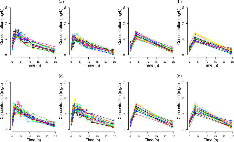
We start considering a parallel design. Two-treatments parallel trials are simulated, that is $20$ subjects receive the reference treatment R and the other $20$ subjects are allocated to the test treatment T. Illustrations of the simulated concentrations in groups R and T under $H_{0}$ and $H_{1}$ in (4.8) are presented in Figure $1$. Secondly, we observe a two-periods two-sequences crossover design. For each trial, the $20$ subjects allocated to the first sequence receive the reference treatment first and then the test treatment. The other $20$ subjects allocated to the second sequence receive treatments in the reverse order. Table 1 displays all variabilities under consideration.

References

- Berger, (1982) Berger, R. L. (1982). Multiparameter hypothesis testing and acceptance sampling. Technometrics, 24:295–300.
- Bristol, (1993) Bristol, D. R. (1993). Probabilities and sample sizes for the two one-sided tests procedure. Communications in Statistics-Theory and Methods, 22(7):1953–1961.
- Brown et al., (1997) Brown, L. D., Hwang, J. G., and Munk, A. (1997). An unbiased test for the bioequivalence problem. The annals of Statistics, pages 2345–2367.
- Chow and Liu, (1992) Chow, S.-C. and Liu, P.-J. (1992). Design and Analysis of Bioavailability and Bioequivalence Studies. Marcel Dekker, New York.
- Combrink et al., (1997) Combrink, M., McFadyen, M., and Miller, R. (1997). A comparison of the standard approach and the nonmem approach in the estimation of bioavailability in man. Journal of pharmacy and pharmacology, 49(7):731–733.
- Comets et al., (2011) Comets, E., Lavenu, A., and Lavielle, M. (2011). Saemix, an r version of the saem algorithm. In 20th meeting of the Population Approach Group in Europe, Athens, Greece. Abstr, volume 2173.
- Demidenko, (2013) Demidenko, E. (2013). Mixed models: theory and applications with R. John Wiley & Sons.
- Dubois et al., (2012) Dubois, A., Gsteiger, S., Balser, S., Pigeolet, E., Steimer, J. L., Pillai, G., and Mentré, F. (2012). Pharmacokinetic similarity of biologics: analysis using nonlinear mixed-effects modeling. Clin. Pharmacol. Ther., 91(2):234–242.
- Dubois et al., (2011) Dubois, A., Lavielle, M., Gsteiger, S., Pigeolet, E., and Mentré, F. (2011). Model-based analyses of bioequivalence crossover trials using the stochastic approximation expectation maximisation algorithm. Statistics in medicine, 30(21):2582–2600.
- Ekstrom, (2019) Ekstrom, C. (2019). Mess: Miscellaneous esoteric statistical scripts. R package version 0.5.5, available at https://CRAN.R-project.org/package=MESS.
- EMA, (2014) EMA (2014). Guideline on the investigation of bioequivalence. available at http://www.ema.europa.eu/docs/en_GB/document_library/Scientific_guideline/2010/01/WC500070039.pdf.
- Gabrielsson and Weiner, (2001) Gabrielsson, J. and Weiner, D. (2001). Pharmacokinetic and pharmacodynamic data analysis: concepts and applications, volume 2. CRC Press.
- Hu et al., (2004) Hu, C., Moore, K. H., Kim, Y. H., and Sale, M. E. (2004). Statistical issues in a modeling approach to assessing bioequivalence or pk similarity with presence of sparsely sampled subjects. Journal of pharmacokinetics and pharmacodynamics, 31(4):321–339.
- Kuhn and Lavielle, (2005) Kuhn, E. and Lavielle, M. (2005). Maximum likelihood estimation in nonlinear mixed effects models. Computational Statistics & Data Analysis, 49(4):1020–1038.
- Lacey et al., (1997) Lacey, L., Keene, O., Pritchard, J., and Bye, A. (1997). Common noncompartmental pharmacokinetic variables: are they normally or log-normally distributed? Journal of biopharmaceutical statistics, 7(1):171–178.
- Lehmann and Romano, (2006) Lehmann, E. L. and Romano, J. P. (2006). Testing statistical hypotheses. Springer Science & Business Media.
- Lixoft, (2018) Lixoft (2018). The monolix software, version r2.
- Mentré et al., (2001) Mentré, F., Dubruc, C., and Thénot, J.-P. (2001). Population pharmacokinetic analysis and optimization of the experimental design for mizolastine solution in children. Journal of pharmacokinetics and pharmacodynamics, 28(3):299–319.
- Midha and McKay, (2009) Midha, K. K. and McKay, G. (2009). Bioequivalence; its history, practice, and future.
- Oehlert, (1992) Oehlert, G. W. (1992). A note on the delta method. The American Statistician, 46(1):27–29.
- Panhard and Mentré, (2005) Panhard, X. and Mentré, F. (2005). Evaluation by simulation of tests based on non-linear mixed-effects models in pharmacokinetic interaction and bioequivalence cross-over trials. Statistics in medicine, 24(10):1509–1524.
- Panhard et al., (2007) Panhard, X., Taburet, A.-M., Piketti, C., and Mentré, F. (2007). Impact of modelling intra-subject variability on tests based on non-linear mixed-effects models in cross-over pharmacokinetic trials with application to the interaction of tenofovir on atazanavir in hiv patients. Statistics in medicine, 26(6):1268–1284.
- Pentikis et al., (1996) Pentikis, H. S., Henderson, J. D., Tran, N. L., and Ludden, T. M. (1996). Bioequivalence: individual and population compartmental modeling compared to the noncompartmental approach. Pharmaceutical research, 13(7):1116–1121.
- Phillips, (1990) Phillips, K. F. (1990). Power of the two one-sided tests procedure in bioequivalence. Journal of pharmacokinetics and biopharmaceutics, 18(2):137–144.
- Romano et al., (2005) Romano, J. P. et al. (2005). Optimal testing of equivalence hypotheses. The Annals of Statistics, 33(3):1036–1047.
- Schuirmann, (1987) Schuirmann, D. J. (1987). A comparison of the two one-sided tests procedure and the power approach for assessing the equivalence of average bioavailability. Journal of pharmacokinetics and biopharmaceutics, 15(6):657–680.
- Sheiner and Wakefield, (1999) Sheiner, L. and Wakefield, J. (1999). Population modelling in drug development. Statistical methods in medical research, 8(3):183–193.
- Tsai et al., (2014) Tsai, C.-A., Huang, C.-Y., and Liu, J.-p. (2014). An approximate approach to sample size determination in bioequivalence testing with multiple pharmacokinetic responses. Statistics in medicine, 33(19):3300–3317.
- U.S. Food and Drug Administration, (2003) U.S. Food and Drug Administration (2003). Guidance for industry: bioavailability and bioequivalence studies for orally administered drug products-general considerations. Food and Drug Administration, Washington, DC. available at http://www.fda.gov/downloads/Drugs/GuidanceComplianceRegulatoryInformation/Guidances/ucm070124.pdf.
- Wellek, (2010) Wellek, S. (2010). Testing statistical hypotheses of equivalence and noninferiority. CRC Press.
- Yee, (2015) Yee, T. W. (2015). Vector Generalized Linear and Additive Models: With an Implementation in R. Springer, New York, USA.
Appendix A Theoretical comparison of tests for bioequivalence
In this section we provide some theoretical explanation, why the approach presented in Section 2.2 has more power than the TOST. For this purpose we now assume that variances in the reference and treatment group are known. In this case the quantiles of the -distribution in (2.7) can be replaced by those of a normal distribution and the power functions of all tests can be calculated explicitly. We also note that this assumption is very well justified, if the sample sizes in both groups are sufficiently large. In other words: all arguments presented in this section can be applied to the NCA-based tests discussed in Section 2.1 and 2.2 provided that the sample sizes are sufficiently large. A similar comment applies to the model-based test for bioequivalence introduced in Section 3. We begin with a discussion of the TOST.
A.1 The two one-sided Test (TOST)
Consider the rejection rule of the TOST defined in (2.7), where we replace the estimate of the (pooled) variance by its true value and the quantile by the quantile of the standard normal distribution denoted by . If the probability of rejection is (because the conditions in (2.7) are contradicting). On the other hand, and more importantly, if the probability of rejection for the test (2.7) is given by