Geometric modeling of M87* as a Kerr black hole
or a non-Kerr compact object
Abstract
Context. The Event Horizon Telescope (EHT) collaboration recently obtained first images of the surroundings of the supermassive compact object M87* at the center of the galaxy M87. This provides a fascinating probe of the properties of matter and radiation in strong gravitational fields. It is important to determine from the analysis of these results, what can and what cannot be inferred about the nature of the spacetime around M87*
Aims. We want to develop a simple analytic disk model for the accretion flow of M87*. Compared to general-relativistic magnetohydrodynamic (GRMHD) models, it has the advantage of being independent of the turbulent character of the flow, and controlled by only few easy-to-interpret, physically meaningful parameters. We want to use this model to predict the image of M87* assuming that it is either a Kerr black hole, or an alternative compact object.
Methods. We compute the synchrotron emission from the disk model and propagate the resulting light rays to the far-away observer by means of relativistic ray tracing. Such computations are performed assuming different spacetimes (Kerr, Minkowski, non-rotating ultracompact star, rotating boson star or Lamy spinning wormhole). We perform numerical fits of these models to the EHT data.
Results. We discuss the highly-lensed features of Kerr images and show that they are intrinsically linked to the accretion-flow properties, and not only to gravitation. This fact is illustrated by the notion of secondary ring that we introduce. Our model of spinning Kerr black hole predicts mass and orientation consistent with the EHT interpretation. The non-Kerr images result in similar quality of the numerical fits and may appear very similar to Kerr images, once blurred to the EHT resolution. This implies that a strong test of the Kerr spacetime may be out of reach with the current data. We notice that future developments of the EHT could alter this situation.
Conclusions. Our results show the importance of studying alternatives to the Kerr spacetime in order to be able to test the Kerr paradigm unambiguously. More sophisticated treatments of non-Kerr spacetimes, and more advanced observations, are needed in order to go further in this direction.
Key Words.
Physical data and processes: Gravitation – Accretion, accretion discs – Black hole physics – Relativistic processes – Galaxies: individual: M871 Introduction
The galaxy Messier 87 (M87) is a giant elliptical galaxy located in the Virgo cluster, first observed by the French astronomer Charles Messier in 1781. Since a century it has been known to give rise to a kiloparsec-scale radio jet (Curtis 1918). The central engine of this jet is likely a supermassive black hole, M87*. It is, like our Galactic Center, a low-luminosity galactic nucleus, displaying a hot, optically thin and most likely geometrically thick accretion/ejection flow (Yuan & Narayan 2014). The distance to M87 is of the order of the mean distance to the Virgo cluster, that is Mpc (Mei et al. 2007). The mass of M87* has been assessed to be M⊙ by means of gas-dynamics fitting (Walsh et al. 2013) and to M⊙ by means of stellar-dynamics study (Gebhardt et al. 2011).
The Event Horizon Telescope (EHT) collaboration has recently published the first reconstructed millimeter images of the close vicinity of M87* (21). The images show a circular crescent feature with a diameter of as, with a non-isotropic flux distribution, surrounding a central fainter region. These features are in good agreement with what is known from theoretical imaging of black holes (Bardeen 1973; Luminet 1979; Marck 1996; Chan et al. 2015; Cunha & Herdeiro 2018). The crescent morphology of the source was constrained by ”free-form” imaging (22), simple geometric models, as well as direct fitting to GRMHD simulations (23). The large collection of GRMHD simulations created a framework for the physical interpretation of the EHT results (24; 53). This analysis allowed to interpret the as circular feature as a lensed accretion/ejection flow within a few from the black hole. The non isotropy can be linked to a relativistic beaming effect. The central fainter region is consistent with being the shadow of the black hole (Falcke et al. 2000). Within this framework, the mass of M87* was estimated to be M⊙, assuming a distance of Mpc (21), which is in agreement with the independent stellar dynamics measurement. For the images shown in this article, we use the consistent values of M⊙ for the mass and Mpc for the distance, following the choice made in 24.
The assumptions of the GRMHD-based analysis and interpretation have given rise to theoretical investigations regarding the nature of the features seen in the EHT images (Gralla et al. 2019; Johnson et al. 2019; Narayan et al. 2019; Gralla & Lupsasca 2019). The main question is to what extent these features can be directly linked to gravitation, and how much are they influenced by the highly model-dependent astrophysics of the emission. There are at least several effects to consider in this context, corresponding to particular choices and simplifications made in the EHT’s GRMHD simulations library (Porth et al. 2019, and references therein). Those include, but are not limited to utilizing a prescription for electron temperature, ignoring the dynamical feedback of radiation, viscosity, resistivity and the presence of non-thermal electrons (24). Apart from that, the turbulent character of the flow adds time dependence to the model, with poorly understood, possibly strongly resolution–dependent, relationship between the simulations and real variability of the source (White et al. 2019, see, e.g.,). Given all those uncertainties, it is both interesting and important to interpret the EHT measurements in the framework of simple physically motivated geometric models. So far, such models have not been extensively discussed in the context of the M87* image interpretation. Only Nalewajko et al. 2020 have recently adopted a geometric model, but with a simple powerlaw prescription for the emission, and no absorption.
Models for M87* environment have been published, using both analytical or GRMHD descriptions of the flow. Analytical models used disk-dominated radiatively inefficient accretion flows (RIAF) or RIAF+jet models (Yuan 2000; Di Matteo et al. 2003; Broderick & Loeb 2009). GRMHD models are describing the disk+jet environment of M87* (Dexter et al. 2012; Mościbrodzka et al. 2016; Davelaar et al. 2019).
The aim of this paper is to contribute to the physical interpretation of the EHT images by using a simple analytical geometric model that is able to capture the most prominent features of a more realistic setup, avoiding the uncertain astrophysics embedded in the latter. For simplicity, we restrict ourselves here to a pure disk model, not taking into account any ejection feature. We stress that the origin of the photons forming the EHT image might be the base of the M87 jet, or the disk. This point was investigated in 24 with a library of state-of-the-art GRMHD simulations. Among a variety of models, only the SANE models, with particularly high parameter (Mościbrodzka et al. 2016), were found to be dominated by the jet emission at that scale. For most of the models, including all MAD ones, the emission observed by the EHT is actually dominated by the disk component. We consider thermal synchrotron emission and absorption in this disk. Our geometric model of the plasma surrounding the black hole is as simple as possible. This simplicity allows to be as little sensitive as possible to the uncertainties that affect more elaborate models. We believe that such a framework is well adapted for testing the impact of the central compact object’s gravitation on the observables. Our goals are to (1) discuss the prominent Kerr image features obtained within this context with a particular emphasis on the accretion-model dependence of the highly-lensed regions, and (2) try to answer the question whether the EHT images, analyzed independently of a broader astrophysical context and of external constraints, can deliver a test of the Kerr-spacetime paradigm. For that purpose we compare the accretion disk images computed for several different models of spacetime. While certain non-Kerr spacetimes were briefly discussed in 21 and 24, all quantitative considerations by the EHT consortium were performed within the framework of the Kerr spacetime paradigm. We aim to fill this gap with the current paper. We highlight that throughout this article, we always consider that gravitation is described by general relativity. While we consider different spacetimes, that may require exotic form of the stress-energy tensor, the Einstein’s theory of gravitation is never modified.
This paper is organized as follows: section 2 considers that M87* is a Kerr black hole. After introducing our disk model in section 2.1, we present millimeter-wave Kerr images in section 2.2, where we discuss the origins of these images main features, related to the properties of highly-bent null geodesics. Section 2.3 briefly discusses the modification in the image generated by non-axisymmetric structures. Section 3 is dedicated to studying how the M87* image changes when the spacetime is different from Kerr. We consider the Minkowski spacetime (section 3.1), the spacetime of a static ultracompact star with an emitting surface (section 3.2), a rotating boson–star spacetime (section 3.3), and a Lamy wormhole spacetime (section 3.4). In section 4, we discuss fits to the EHT data of our Kerr and non-Kerr models. Section 5 gives conclusions and perspectives.
2 Emission from a thick disk in a Kerr spacetime
In this section, the Kerr spacetime is labeled by means of the Boyer-Lindquist spherical coordinates . We work in units where the gravitational constant and the speed of light are equal to , . Radii are thus expressed in units of the black hole mass .
2.1 Disk model and emission
We consider a geometrically thick, optically thin accretion disk in a setup illustrated in Fig. 1.
For simplicity, we parametrize the geometry of the accretion disk by only two parameters, its inner radius and opening angle . We do not prescribe any outer radius for the disk. It is effectively imposed by selecting a field of view for computing the images, as well as by the radially decaying profiles of temperature and density. The disk is assumed to be axisymmetric with respect to the axis which lies along the black hole spin. The compact object and accretion-disk spins are assumed to be aligned, as is the case for the entire EHT GRMHD library. Throughout this article we fix the opening angle of the to , so the disk is moderately geometrically thick. This choice places our considerations between the limit cases of geometrically thin model considered by Gralla et al. 2019 and spherical accretion considered by Narayan et al. 2019, and within the thickness range expected for a real accretion flow in M87* (Yuan & Narayan 2014).
We model the emission by thermal synchrotron radiation. This is also a simplification because shocks and turbulence in the accretion flow are likely to generate non-thermal emission. However, we chose to neglect this additional complexity. This is again primarily for the sake of simplicity, but also because the broad features of the image are unlikely to be extremely sensitive to the details of the emission process, and because the non-thermal emission modeling would necessarily imply somewhat arbitrary extra assumptions anyway. Thermal synchrotron emission is modeled following the formulas derived by Pandya et al. 2016. Both the emission and absorption coefficients are self-consistently taken into account in our computation. These coefficients depend on the electron number density and temperature, as well as on the magnetic field strength. The parameters of our model are the density and temperature at the inner disk radius, and . We assume simple power laws for their scaling, for the density, and for the temperature, following the description of Vincent et al. 2019.
We do not consider any vertical variation of the accretion flow properties. As for the magnetic field prescription, we simply impose the magnetization , equal to the ratio of the magnetic to particle energy densities, with being the magnetic field magnitude, the proton mass, and the velocity of light (kept here for clarity). This quantity is always set to in this article. This is an arbitrary choice, which has little impact on our results given that we do not discuss a mixed disk+jet model, in which case the magnetization should typically differ in the disk and in the jet. We note that our choice of power laws for the electron density, temperature, and the magnetic field are that of the standard model of Blandford & Königl 1979. It also agrees with the inner evolution of these quantities in GRMHD simulations of M87* (Davelaar et al. 2019, see, e.g.,). We stress that only the inner few tens of of the flow matters for the images that we discuss here. We thus parametrize the radial dependence of the disk quantities in order to capture the relevant properties of this region.
For all the images shown in this article, we assume the observing frequency of GHz, corresponding to the observing frequency of the EHT. The orientation of the model is determined by the assumption that the jet aligns with the black hole / disk spin axis and by the observed jet position angle on the sky. We fix the inclination (angle between the black hole spin and the line of sight) to (Walker et al. 2018), meaning that the black-hole and disk spin vectors are directed ”into the page” for all images presented here (24), see Fig. 1. This nearly face-on inclination may be in general unfavorable for considering deviations in the image geometry, when compared to near-edge-on views (Bardeen 1973). The position angle of the approaching jet (angle east of north of the black hole spin projection onto the observer’s screen plane) is fixed to (Kim et al. 2018). The field of view of the presented images is fixed to as and the number of pixels to (unless otherwise noted).
One extra crucial assumption has to be made: the choice of the dynamics of the accretion flow. We will always consider Keplerian rotation outside of the innermost stable circular orbit (ISCO), irrespective of the height with respect to the equatorial plane. If the inner radius is smaller than , the emitting matter 4-velocity below ISCO is given as
| (1) |
where is the 4-velocity of the zero-angular-momentum observer (ZAMO) and is the accretion flow velocity as measured by the ZAMO. It can be written as
| (2) |
so that . This velocity is parametrized by choosing and . In the following, we always fix to its value at the ISCO. For the two spin-parameter values considered, and , this gives respectively and . We can then chose to simulate a limit case corresponding either to a flow with purely circular velocity (if ), or a radially plunging flow (if ). Note that the emitter velocity is always independent of the height , defined using Boyer-Lindquist coordinates by .
We ensure that the observed flux is of the order of Jy, in agreement with the state of M87* at the time of the 2017 EHT campaign. The flux is primarily impacted by the choice of the electron number density and temperature at the inner radius. Given that these two quantities are degenerate because we are fitting a single flux value (rather than the full spectrum), we decide to fix the electron number density at to , which is in reasonable agreement with the results published in the literature by various authors (Broderick & Loeb 2009; Davelaar et al. 2019, 24). The number density at the chosen value of is thus fixed by the assumed density scaling. The inner temperature is then chosen to obtain a reasonable value of the observed flux. We find that the choice of K (or in units of the electron rest mass) leads to reasonable flux values for all setups considered here.
The final step of our simulation is to perform general-relativistic ray tracing, either in the Kerr spacetime or in other geometries, to obtain theoretical images. This is done using the open-source ray tracing code Gyoto (see Vincent et al. 2011; Vincent et al. 2012, and http://gyoto.obspm.fr) to compute null geodesics backwards in time, from a distant observer located at the distance of Mpc away from the disk. We summarize the fixed properties of the model and images in Table 1.
| Symbol | Value | Property |
|---|---|---|
| 6.2 M⊙ | compact object mass | |
| 16.9 Mpc | compact object distance | |
| 30∘ | disk opening angle | |
| max number density of electrons | ||
| K | max electron temperature | |
| 0.1 | magnetization | |
| 160∘ | inclination angle | |
| -70∘ | jet position angle east of north | |
| 230 GHz | observing frequency | |
| 160 as | field of view | |
| – | 200200 | image resolution |


2.2 Main features of the images
Figures 2-3 show the Kerr-spacetime disk images obtained for two different values of the spin parameter. In this section, we discuss the main features of these images, focusing on the impact of the flow geometry and dynamics, as well as on the highly-lensed-flux portion of the image, generally loosely called the ”photon ring”.
Figure 2 shows the resulting image for a spin parameter and three different choices for the accretion disk properties. We note that such non-rotating configurations are unlikely to account for the powerful large-scale jet of M87 (24). These configurations are still of interest for a comparison with the rotating ones. The top-left panel shows a Keplerian flow with inner radius at the Schwarzschild spacetime ISCO, . The top-middle panel has an inner radius going down to the event horizon at , with a purely azimuthal velocity below the ISCO (). The top-right panel is the same as the middle panel, but with (pure radial inflow). The bottom panels show the same images, convolved with a Gaussian kernel with full width at half maximum of as, which is approximately the EHT angular resolution (22). In this image, as well as in the following ones, we indicate the approximate position of the crescent feature reported by the EHT, 40 as, with a dashed circle. For the compact object mass and distance assumed in this paper, this translates into diameter. Figure 3 shows the same setup for a spin of , with and .
The unblurred images presented in Figs. 2 and 3 all show thick annular areas with the addition of a very thin bright ring. The thick annular area is due to the emission from the inner parts of the disk, with a feeble lensing effect on the null geodesics. It is generally referred to as the primary image of the disk, and is composed of geodesics that cross the equatorial plane at most once (Luminet 1979). The polar radius of the primary image clearly varies with the assumed . The brightness distribution with azimuthal angle in the primary image is a consequence of the special-relativistic beaming effect: parts of the flow coming towards the observer are boosted. This effect is clearly visible in the left and central upper panels of Fig. 2 where the flow is in circular rotation and coming towards the observer in the south direction. The upper-right panel of the same figure is obtained when the inner radius is set at the event horizon and the flow velocity is chosen to be purely radial below the ISCO. In this case, the flux distribution is less dependent on the azimuth than for the circularly-rotating cases. We have however checked that, when taking into account special-relativistic effects only, the image becomes boosted in the west direction where the flow approaches the observer. The blurred image of this radial-inflow case (lower-right panels of Figs. 2) is thus very isotropic, which is not consistent with the observed EHT image. This elementary discussion shows that the size of the primary image and its flux distribution with azimuthal angle are directly linked to the choice of the inner radius and to the dynamics of the gas in the inner disk regions. This result agrees with that obtained by Nalewajko et al. 2020 with a simpler model.
The very thin bright ring, also present in the unblurred images, is often loosely referred to as the photon ring, and considered to be the image on sky of the unstable Kerr equatorial prograde photon orbit. However, the set of orbits that actually matters in order to form this highly lensed feature is the set of spherical Kerr photon orbits first analyzed by Teo 2003, with numerous recent developments (Cunha et al. 2017b; Johnson et al. 2019, see, e.g.,). These are bound unstable photon orbits evolving at constant Boyer-Lindquist radii, with periodical excursion in the direction (the span of this excursion, , depends on the photon’s angular momentum). The orbits are not periodic in and are either prograde or retrograde, depending on the sign of the photon’s conserved angular momentum. These orbits exist within a radial range , where and are the usual Kerr equatorial prograde and retrograde photon orbit radii. In particular, for the Schwarzschild spacetime in which only one photon orbit exists at , the set of spherical photon orbits is simply the sphere . The thin bright ring in Kerr images is thus due to light rays that approach a spherical Kerr photon orbit before reaching the far-away observer.
As stated above, the spherical Kerr photon orbits are periodic in . The complete excursion from to (or the other way round) can be covered by a null geodesic an arbitrary number of times , corresponding to crossings of the equatorial plane, before leaving the orbit and reaching the far-away observer (remember that these orbits are unstable). As increases, the Boyer-Lindquist radius of such an orbit becomes very close to that of a spherical photon orbit and the impact point on sky tends to the critical curve. Thus, the thin bright ring is actually the sum of an exponentially converging sequence of sub-rings lying at smaller and smaller polar radii on sky, and labeled by the number of crossings of the black hole equatorial plane (see Figure 5). This fact was first noted by Luminet 1979 for the Schwarzschild case. The resolution of the image truncates this sequence at a finite number of sub-rings (see, e.g., the lower-right panel of Fig. 6 where the outermost sub-ring is clearly seen, the subsequent sub-ring is only barely visible, and the following ones are lost due to finite resolution). Note that for the M87* image, the complete set of sub-rings of the thin bright ring lies within as on sky so that a very high resolution would be needed to resolve some of its components. Gralla et al. 2019 use the term lensing ring for the outermost such sub-ring (corresponding to the set of geodesics that cross the equatorial plane exactly twice), while they keep the terminology photon ring for the sum of all subsequents sub-rings (corresponding to the set of geodesics that cross the equatorial plane more than twice).
Johnson et al. 2019 give an analytic expression for the limiting curve on sky, towards which the series of sub-rings converge in the limit of . This limiting curve was called the critical curve by Gralla et al. 2019 and we keep this name. Introducing – the polar radius on the observer’s screen in units of , and – the polar angle on the observer’s screen, the critical curve reads
| (3) | |||||
where
| (4) | |||||
Here, is the Boyer-Lindquist radius of the Kerr spherical photon orbit followed by the photon on its way to the observer. One counter-intuitive property of this critical curve, already discussed by Johnson et al. 2019, is the fact that one Kerr spherical photon orbit (one value of ) is mapped to 2 values of the polar angle, and . This is due to the arccos definition of . As a consequence, the critical curve should be seen as the image on the sky of the set of Kerr spherical orbits, with each spherical orbit being mapped to 2 points along the curve. Note that actually only a subset of the full set of Kerr spherical photon orbits () is imaged on the sky, depending on the value of the inclination . Only for does the full set get imaged on the sky (Johnson et al. 2019, see Fig. 2 of).
In this article, we are interested in the full sequence of highly-lensed sub-rings on the sky, which incorporates the notions of the lensing ring, the photon ring, and the critical curve introduced above. However, it is crucial to realize that a pixel on the observer’s camera belonging to one of this sub-rings will not always contain a detectable amount of flux. Its flux content, and hence its ability to be considered as a highly-lensed region on sky, depends on the corresponding null geodesic interaction with the accretion flow. As a consequence, the full set of highly-lensed sub-rings should be seen as a mathematical, theoretical locus on sky, the flux content of which fully depends on the accretion flow properties. We thus introduce the observation-oriented notion of the secondary ring (as opposed to the primary image) to refer to the region on the observer’s sky where the received null geodesics (i) have approached a Kerr spherical photon orbit within in terms of the radial Boyer-Lindquist coordinate , and (ii) have visited the regions of the accretion flow emitting most of the radiation. In this definition, can be of order for lensing-ring photons, while for photon-ring photons (see the lower panels of Fig. 4). The regions of the flow emitting most of the radiation, in our framework, coincide with the inner regions close to , where all physical quantities are maximal. We note that this definition implicitly depends on the orientation of the observer with respect to the flow. Indeed, the projection on sky of the regions of the flow emitting most of the radiation depends on the inclination and position angle.
Our definition is based on more than just the number of crossings of the equatorial plane by null geodesics. As discussed in the Appendix A, a definition based only on the number of crossings of the equatorial plane is not adequate as geodesics can cross this plane at very large radii, and such crossings are not relevant for the definition of the secondary ring. Moreover, and most importantly, the secondary ring definition must be linked to the particular accretion flow model used and its emission law. This crucial point is illustrated in Fig. 4, which shows the link between the Kerr spherical orbits, the accretion flow geometry, and the secondary ring of the image.
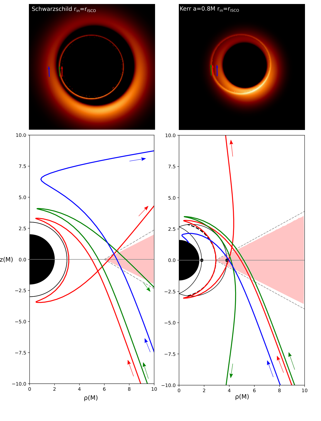
It first shows that highly-lensed geodesics (with more than 2 crossings of the equatorial plane close to the black hole) indeed approach a Kerr spherical orbit in the vicinity of the black hole. Most importantly, it also shows that not all geodesics that approach Kerr spherical orbits will correspond to bright pixels of the image. A secondary-ring geodesic is not only highly bent, but it is also selected by the fact that it should visit the inner parts of the accretion flow in order to transport enough flux (the red geodesic of the lower-right panel of Fig. 4 is a good example: its spherical-orbit radius is exactly equal to the radius of the bright inner edge of the disk, allowing to transport a lot of flux). Consequently, both the polar radius on sky and the azimuthal flux distribution of the secondary ring are depending on the properties of the accretion flow; they are not simply dictated by gravitation. Should the inner radius of the disk of the lower-right panel of Fig. 4 be moved down to the event horizon, the red geodesic would transport a much smaller amount of flux, and would thus not be considered as belonging to the secondary ring (the geodesic optical path within the flow would be longer, but this increase scales as , while the decrease in density scales as , so that the resulting flux would be smaller). It has been recently shown by Gralla & Lupsasca 2019 that the dependence of the lensing ring polar radius on the accretion flow geometry can reach tens of percent (see their Fig. 5). We note that this result, obtained for a geometrically-thin disk, should be considered as a lower limit in a geometrically-thick disk context.
Figure 5 illustrates the notion of secondary ring and highlights its dependence on the properties of the plasma surrounding the black hole.
Four important notions have been introduced so far: lensing, photon and secondary rings, and the critical curve; some of which having non-trivial definitions. Figure 6 gives a pedagogical illustration of these notions. We insist on the fact that the only new word that we introduce here, i.e. the notion of secondary ring, is really needed. Indeed, it conveys the crucial idea that highly-lensed features in the image plane are intrinsically depending on the astrophysical accretion model, which does not appear clearly in the definition of other notions (lensing, photon rings).

Let us now discuss more quantitatively our Kerr images. We note that in Figs. 2 and 3, the angular size of the dark central region depends a lot on the inner radius of the accretion flow. This is in agreement with the simple model of Gralla et al. 2019. In particular, the secondary ring is not the outer boundary of this central dark region when the flow extends to the horizon. On the other hand, Narayan et al. 2019 recently showed that a spherical optically thin flow in a Schwarzschild spacetime results in a central dark region the angular size of which is independent of the location of the inner edge of the emitting region. This discrepancy once again highlights the importance of the careful modeling of the accretion flow for the interpretation of EHT images.
It is also interesting to determine the brightness ratio of the secondary ring to the primary image. We have checked that in the non-rotating case, the secondary ring weight is of when , when with azimuthal flow velocity, and when with radial flow velocity. For the case, the secondary ring weight is of when , when with azimuthal flow velocity, and when with radial flow velocity. These numbers are obtained following the methodology presented in Appendix A. As explained there, they should be considered as slightly over-estimated. For comparison, Johnson et al. 2019 characterize the secondary ring to be responsible for of the total flux seen in ray-traced GRMHD simulations, with specifically a weight of reported for their Fig. 1. Our results are thus in good agreement with the more sophisticated GRMHD simulations.
2.3 Non-axisymetric emission
The flux distribution seen in Fig. 2 and 3, with the south region of the image brighter than the north part, is primarily due to the beaming effect. This is so because the emission is assumed to be axisymmetric. However, non-axisymmetric flux distribution is necessarily present in realistic turbulent flows. It is thus a natural question to ask what should be the condition on the non-axisymmetry of the emission such that the flux repartition would be substantially altered. To investigate this point, we study a very simple non-axisymmetric feature in our disk model. We consider that some region of the disk, centered at a cylindrical radius (defined in Boyer-Lindquist coordinates by ) of and azimuth , with typical extensions and , will be hotter than the rest by some increment . Specifically, we consider that the temperature around will read
| (5) |
where is the axisymmetric temperature defined in the previous section, , is a chosen parameter, and the function is the following product of Gaussians
| (6) |
To enhance the difference with respect to the axisymmetric case, we choose such that this region is located towards the north on the sky, i.e., opposed to the beamed region. The parameters and are chosen such that the hotter region has a comparable extension on the sky as compared to the beamed region of the axisymmetric images.
Fig. 7 shows the images obtained when is varied.

The images indicate that the temperature has to increase by a factor of around in order for the non-axisymmetric structure to overcome the beaming effect. Seeing such an unusually hot coherent component in the GRMHD simulations is rather uncommon. This can be seen in Fig. 9 of 24, where a collection of GRMHD snapshots fitted to the EHT data create a distribution centered around an expected brightness maximum position angle of (about 90∘ clockwise from position angle of the approaching jet projection) with turbulence related scatter of . Nevertheless, there is a non-zero probability for a very different fitted orientation. It is not entirely clear how accurate are GRMHD models at reproducing the intrinsic turbulence-induced structural variability of a realistic accretion flow in the vicinity of a black hole, as EHT is the first instrument to deliver observational data that could be used to test this.
3 Emission from a geometrically thick disk in non-Kerr spacetimes
In this section, we present millimeter images of a geometrically thick disk surrounding compact objects that are different from the standard Kerr black hole. We will first focus on non-rotating solutions (Minkowski and ultracompact star spacetimes, see sections 3.1 and 3.2) and then on rotating solutions (boson star and Lamy wormhole spacetimes, see sections 3.3 and 3.4). Our goal is to determine whether or not the current EHT data can exclude non-Kerr spacetimes based on arguments independent of the geometric structure of the accretion flow. This section presents theoretical images, while the fits to EHT data are discussed in section 4.
3.1 Minkowski spacetime
We start by considering the most extreme non-Kerr case of a flat spacetime described by Minkowski geometry. While there may be little physical motivation to consider such an object as a viable alternative to a Kerr black hole, with this exercise we investigate whether any spacetime curvature is absolutely necessary to explain the EHT images. This means that we only consider the laws of special relativity but discard all general relativistic effects. This describes what could be thought of as a Michell-Laplace relativistic black hole (Michell 1784; Laplace 1796). It is a ”relativistic” black hole because of the important addition of special relativity as compared to the original object. We want to compare this ”flat-spacetime black hole” to a Schwarzschild black hole. In both cases, an accretion disk is assumed to lie in the equatorial plane of the object, with the same inner radius . There is of course no physical motivation to terminate the accretion disk at this radius for our Michell-Laplace relativistic black hole. Our choice is dictated by the comparison to the Schwarzschild spacetime. The angular velocity of the emitting matter of the Michell-Laplace relativistic black hole is assumed to follow the Newtonian law .
Figure 8 shows a comparison between these two cases.

The high resolution images can be immediately distinguished by the absence of a secondary ring in the Minkowski spacetime. We return to that aspect in section 5.2, discussing future observational perspectives. Nevertheless, the extreme similarity between the images observed with the EHT resolution (bottom row of Fig. 8) is a good illustration that reasoning based exclusively on the image morphology can tell little about the nature of the central object.
3.2 Non-rotating ultracompact star

We compute here the image of M87* assuming that the central compact object is not a black hole but rather an ultracompact non-rotating star with a surface slightly above the radius of its event horizon. While we refer to this hypothetical object as a “star”, its only assumed property is the presence of a surface, as we do not consider any internal physics of the object. Birkhoff’s theorem ensures that the metric at the exterior of this object will be the Schwarzschild metric, provided the ultracompact star is spherically symmetric. We note that, should the star rotate, its exterior metric will not be in general that of Kerr so that the generalization to a rotating spacetime is not straightforward.
Our ultracompact-star spacetime is defined as follows. The star surface is modeled as a spherical surface of Boyer-Lindquist radial coordinate with in a Schwarzschild spacetime. The star’s surface is assumed to be fully optically thick so that its interior (which is not properly modeled in our setup) is never visited by any photon.
The star’s surface is assumed to emit blackbody radiation at the temperature of the inner accretion flow, , here assumed to be K. This is of course a very strong assumption. It is likely, however, that this surface should be thermalized given that null geodesics are highly curved when emitted at the star’s surface and thus efficiently couple different parts of the surface (Broderick et al. 2009). Moreover, the considerations presented here will not be qualitatively affected if the surface temperature is not exactly equal to the inner accretion flow temperature.
Let us now discuss more quantitatively the radiation emitted at the star’s surface. The observing frequency is fixed in the whole article to the EHT observing frequency, GHz. The emitted frequency at the star’s surface is simply related to that by , where is the redshift factor, which decreases to as approaches the Schwarzschild event horizon. The Planck function peaks at a very high frequency of Hz. The emitted frequency reaches this value for . In the following we will thus safely assume that the Planck function is in its Rayleigh-Jeans regime. Using the frame-invariance of , we can thus express the observed specific intensity as
| (7) | |||||
where is the Boltzmann constant, is kept explicitly for clarity, and we have used the assumption that . We want this observed specific intensity, corresponding to the interior of the secondary ring in the ray-traced images of Fig. 9, to be equal to some fraction of the maximum observed specific intensity from the accretion disk, . We thus write
| (8) |
and
| (9) |
When considering a Schwarzschild black hole surrounded by a thick disk with (see Fig. 2, top-left panel), the maximum observed specific intensity from the accretion disk is of the order of Jy srad-1. Fixing (the stellar surface emission is negligible), corresponding to the dynamic range of the EHT images (22), we derive , and for (the stellar surface dominates) we find . The following equation gives a practical expression for
| (10) |
that can be understood as a joint constraint on and the surface temperature. Figure 9 shows the image of an accretion disk with surrounding a Schwarzschild black hole (left panel), and an ultracompact star with surface radius defined by (middle panel) or (right panel). Provided that is small enough, there is no noticeable difference between the Schwarzschild and ultracompact-star cases. We bring up future perspectives of constraining in section 5.3.
Although we do not discuss gravastars (Mazur & Mottola 2004) in this article, we note that non-rotating gravastars would lead to similar images as our Fig. 9, because in both cases a near-horizon surface is present and the external spacetime is Schwarzschild.
3.3 Rotating boson star
In this section, we consider the spacetime of a rotating boson star, as computed by Grandclément et al. 2014. We are modeling what is known as a mini boson star, in the sense that we do not consider any self-interaction between the bosons. Boson stars are composed of an assembly of spin-0 bosons consituting a macroscopic quantum body that evades collapse to a black hole by means of Heisenberg uncertainty relation (Liebling & Palenzuela 2017). Boson stars have no hard surface, no event horizon, and no central singularity. As such they are extremely different from black holes and are a good testbed for horizonless spacetimes (Vincent et al. 2016).
A boson star is defined by two parameters, and (see Grandclément et al. 2014, for details; note that is in units of where is the mass of the boson). The angular momentum of a boson star is quantized and proportional to the integer because of the quantum nature of the object. The parameter is related to the compactness of the star, with compactness increasing when approaches . Here, we consider a boson star defined by , which has already been discussed in Vincent et al. 2016. For boson stars may or may not have photon orbits depending on the value of (Grandclément 2017). If photon orbit exist, there must exist at least two of them, one of them being stable, leading to a questionable stability of the spacetime (Cunha et al. 2017a, this statement is actually much more general and applies to any axisymmetric, stationary solution of the Einstein field equations with a matter content obeying the null energy condition). The boson star spacetime is interesting because there is no known reason to question its stability. In particular, it has niether a stable photon orbit, nor an ergoregion. Its parameters translate to a spin of , the same as the Kerr black hole discussed in section 2.
Figure 10 shows a comparison between the image of a geometrically thick accretion disk surrounding a Kerr black hole and the rotating boson star discussed above.

For the Kerr spacetime, the inner radius of the accretion disk is fixed at the ISCO, . For the boson star spacetime, using the same inner radius leads to a slightly too small image on sky. We thus increased it to in order to match as closely as possible the Kerr image. The inner number density is chosen accordingly, following our power law. Choosing a different inner radius for the two spacetimes is not an issue, our goal being only to determine whether a boson-star spacetime can mimick a Kerr spacetime. The emitting matter of the boson star spacetime is following circular timelike geodesics of the boson-star metric, the equation of which can be found in Grandclément et al. 2014. These authors have analyzed the stability of timelike circular geodesics for boson stars. They show that all circular timelike geodesics are stable for boson stars, so that it is sufficient to speak of the innermost circular orbit (ICO). Our boson star has an ICO at . Our choice of means that the inner disk radius is at times the ICO radius for the boson star spacetime. For comparison, we also show the image corresponding to a choice of in the right column of Fig. 10.
The boson-star case with a larger inner radius of the accretion flow leads to a blurred image very similar to Kerr, given that the thin secondary ring of the Kerr image is washed out by the limited resolution of the observations. On the other hand, setting the inner radius at the ICO leads to a much smaller image on sky (assuming the same mass), which results in a blurred image very different from Kerr. This shows that it is the accretion flow properties that matter when comparing a boson star to a Kerr black hole. Modifying the spacetime geometry alone is not sufficient in order to produce an observationally different image independently on the accretion flow geometry. This demonstrates that more sophisticated simulations, connecting general relativity and the accretion flow magnetohydrodynamics, may be necessary to convincingly discuss the observable differences between black holes and other compact objects.
Recently, Olivares et al. 2018 published the first GRMHD simulation of an accretion flow surrounding a non-rotating boson star. They computed the associated GHz image, taking into account physical parameters typical of the Sgr A* environment, concluding that it is possible to distinguish a boson star from a black hole by comparing the non-rotating boson-star image to a Schwarzschild and Kerr images. They reported the boson-star image to be more compact and symmetric, similarly as the results we present in the last column of Fig. 10, as a consequence of a gas accumulation at small radii. However, this picture may be different for a fast-spinning boson star (notice, that there are no slow-rotating boson stars). Answering this question requires further GRMHD studies, that might in particular be able to discuss the jet power delivered by a boson star.
3.4 Lamy spinning wormhole
In this section we consider the rotating wormhole solution first described in Lamy et al. 2018, that we will hereafter refer to as Lamy wormhole. This solution was found by generalizing the spherically-symmetric regular (i.e. singularity-free) black hole solution of Hayward 2006 to the rotating case. This metric takes the same form as the Kerr metric expressed in Boyer-Lindquist coordinates, but with the constant replaced by the function
| (11) |
where is a charge homogeneous to a length (it is expressed in units with our conventions). In the original Hayward metric, is interpreted as a scale at which quantum gravity effects would act and regularize the classical singularity. It should therefore typically take extremely small values. However, this parameter has been reinterpreted by Fan & Wang 2016 as the magnetic charge associated to a magnetic monopole in a nonlinear electrodynamics theory that sources the Hayward metric. In this context, can take macroscopic values.
Here, we consider only one pair of values for the spin parameter and charge, and . This choice fully specifies the metric. It can be shown that this spacetime corresponds to a rotating wormhole (Lamy et al. 2018). In particular, it has no event horizon, and of course no curvature singularity. The topology of this spacetime corresponds to two asymptotically flat regions, one with and one with , connected by a throat at . The energy conditions are violated in the full region , however the stress-energy tensor decreases fast to zero when increases so that the exotic matter is concentrated near the throat. This spacetime is very exotic. It is, however, quickly converging to Kerr away from (typically, for , the metric is Kerr; the relative difference of for instance is less than in the equatorial plane for ). Thus, a Lamy wormhole can be seen as an interesting testbed for the wormhole-like non-Kerrness of spacetime. The final important property of this spacetime (as well as all Lamy spacetimes) is that they admit spherical photon orbits similar to Kerr’s. Their locus depends of course on the values of and . They are analyzed in Lamy 2018.
Figure 11 shows three images of a thick disk surrounding our Lamy wormhole, compared to a Kerr image. The lower-left panel is interesting in order to understand the highly-lensed central part of the image, as it is not confused with the primary image.

The striking feature of the highly-lensed part of this panel is the existence of two rings, and of a crescent in between the rings. These features are also noticeable in the upper-right panel, although less clear as they overlap with the primary image. These features are due to extreme light bending in the central regions of the Lamy spacetime, due to the existence of spherical photon orbits. They are absent in the boson-star image in Fig. 10, as the , boson star has no photon orbits.
In order to go one step further in the analysis of the impact of photon orbits on the image, we have considered a more compact boson star spacetime, with and , which has been already studied in Vincent et al. 2016. This spacetime has photon spherical orbits. Figure 12 shows null geodesics corresponding to one of the bright pixels of the inner crescent feature of the lower-left panel of Fig. 11 computed in Lamy, Kerr, and the two different boson star spacetimes. It highlights the close similarity of the geodesics corresponding to the two horizonless spacetimes with photon orbits (Lamy in red and boson star with , in black). Both of them lead to a very big change of the Boyer-Lindquist coordinate of the null geodesic before and after approaching the compact object. On the contrary, the horizonless spacetime with no photon orbit (boson star with , , in green) leads to a very different geodesic with much smaller change of when approaching the compact object. Appendix B shows that the similarity between the boson star (, ) and Lamy spacetimes is not restricted to the particular geodesic represented in Fig. 12. The complete images are extremely similar and possess a comparable inner crescent feature (see Appendix B).
Note that such a crescent feature was also noticed for edge-on views in these two spacetimes by Vincent et al. 2016 and Lamy et al. 2018. It is thus plausible that such features are characteristic of a large class of horizonless spacetimes with photon orbits.
Figure 13 compares the EHT-like images obtained for Kerr and Lamy spacetimes.

It shows that the complex features of the Lamy spacetime are partially lost when blurred at the EHT resolution. Still, there is a clear excess of flux in the central fainter region as compared to Kerr. Given that the non-Kerrness of Lamy spacetime depends directly on the charge , it would be possible to derive a constraint on this parameter by performing fits of various Lamy spacetimes with different values of the charge. Such a constraint goes beyond our current analysis.
4 Fitting models to the EHT data
Up to this point we have only discussed the differences between Kerr and non-Kerr images based on qualitative image-domain comparison. It is important to notice that we did not consider the sparsity-related limitations of the EHT image reconstruction capabilities (22). Effectively, our images represented the actual view of the model at the assumed resolution, without any reconstruction-related distortions. In contrast, this section is devoted to comparing models of different compact objects directly to the M87* observational Fourier domain data.
The total intensity data from 2017 EHT observations of M87* have been publicly released11 1 https://eventhorizontelescope.org/for-astronomers/data. The data consist of 4 independent days of observations in 2 independently recorded and processed frequency bands (25, HI and LO,). We performed fitting of the models presented in sections 2-3 to all 8 released EHT datasets. As is the case in very long baseline interferometry (VLBI), data correspond to the sparsely sampled Fourier transform of the images on the sky (Thompson et al. 2017). Because of the sparsity limitations, sophisticated postprocessing is required in order to reconstruct the corresponding image (22). While Fourier domain (referred to as visibility domain in this context) data offer well understood error budget, reconstructed images may suffer from the difficulty to assess systematic uncertainties. This is why all quantitative model fitting should take place in the visibility domain. In our case we are sampling the ideal (unblurred) model images using a synthetic model of the EHT array, utilizing the exact coverage of the M87* observations in the 2017 EHT campaign, and the expected magnitude of uncertainties. That part of the work was performed in the framework of the eht-imaging library (Chael et al. 2016; Chael et al. 2019, http://github.com/achael/eht-imaging). For the crude fitting procedure that we utilize in this paper, we consider scaling, rotation, and blurring of the model images, minimizing the reduced errors calculated against robust interferometric closure quantities (Blackburn et al. 2019b, closure phases and log closure amplitudes,). In each iteration of the error minimization procedure, the updated model is sampled and compared with the observed closure data. The procedure of selecting the linearly independent set of closure data products and defining the exact form of the minimized error functions follows that described in 22 and 23. From the estimated scaling parameter, we recover the mass of the model best fitting the data. The rotation parameter allows to calculate the position angle of the bright feature found in the best-fitting model. Note that both scale and orientation of the image were fixed in the discussions in previous sections to the values given in Tab. 1. The results of the fitting procedure are summarized in Fig. 14. All models individually give very consistent mass estimates for all days and bands, indicating that the errors are not of random statistical character, but rather are dominated by the systematic model uncertainties. Zero-spin models consistently result in much lower estimated mass, roughly consistent with the competing M87* mass measurement based on gas dynamics (Walsh et al. 2013). This is most likely a consequence of the choice of , resulting in a larger image for the fixed object mass than in the case of a smaller . GRMHD simulations suggest that the ISCO has little importance for hot optically thin flows (Yuan & Narayan 2014), hence such a choice of may be seen as inconsistent with the additional astrophysical or magnetohydrodynamical constraints. The models with spin yield object mass consistent with the EHT and with the stellar dynamics measurement (Gebhardt et al. 2011). All models localize the maximum of the emission in the south of the image, see Fig. 14, right panel. The position angle of , which approximates the expected orientation, given the observed position of the jet on the sky (24, jet position angle in the observer’s plane minus 90∘,), is indicated with a dashed horizontal line. We also see indication of counterclockwise rotation between first and last day of the observations, consistently with results reported in 22 and 23. None of the fits are of very high quality, as expected from very simple models with little number of degrees of freedom, see Figure 15, and there is no clear indication of any of the models outperforming others. Some models, such as the ultracompact star with a surface located at 2.05 (Fig. 9, middle column, fitting results not shown in this section) are in dramatic disagreement with the data, resulting in reduced errors larger than 100 for each of the EHT data sets. Similarly, the model of a boson star shown in the last column of Fig. 10, being rather symmetric in appearance, fits data poorly with reduced for all EHT data sets. The fitting errors reported in Figure 15 are of similar magnitude as the average ones resulting from fitting individual snapshots from GRMHD simulations to the EHT data (24). This supports the notion that geometric models could effectively represent mean properties of the more complicated simulations.
5 Conclusion and perspectives
In this article we develop a simple geometric model for the inner accretion flow of M87*, the supermassive black hole at the center of the galaxy M87. We use this model to obtain predictions of the millimeter image of the close surroundings of M87*, and compare them to the EHT findings. We have been focusing mainly on two questions.
First, we tried to develop on the recent studies devoted to improving our understanding of the sharp highly-lensed features of strong-field images (Gralla et al. 2019; Johnson et al. 2019). Our findings regarding this issue are summarized in section 5.1 below.
Secondly, we investigated whether objects alternative to Kerr black holes (be they physically justified or not) could produce observational signatures similar to those seen by the EHT. We have shown that interpreting EHT data sets with geometric flow models results in the image-domain morphology being consistent with the EHT findings (see also Figs. 20-21), and several non-Kerr spacetimes fitting the EHT data similarly well as their Kerr counterparts.
We showed that without an imposed assumption on the compact object mass, no spacetime curvature effects are needed to explain the current EHT results (see Michell-Laplace black hole). Even if a mass prior from stellar dynamics is assumed, exotic objects such as boson stars or Lamy wormholes can provide images consistent with the EHT observations of M87*, with a favorable geometric configuration of the accretion flow. Hence, we conclude that the published EHT observations, while consistent with the Kerr paradigm, do not provide a strong and unambiguous test of its validity. Our results agree also with the general point made earlier by Abramowicz et al. 2002. Although, as stated by these authors, there cannot be any direct electromagnetic proof of the existence of an event horizon, there is a hope for a robust detection of a secondary ring by a more developed future version of the EHT. This would be of great importance, showing the existence of null spherical orbits (which is however still very different from showing that the object is a Kerr black hole). On the other hand, resolving sharp, strongly lensed image features inconsistent with the ring geometry, such as what is seen for horizonless spacetimes with photon orbits (see Appendix B), would make a very strong argument against the Kerr paradigm. Sections 5.2 and 5.3 below are giving our main conclusions regarding these topics. Finally, section 5.4 gives some future research perspectives.
5.1 Definition of the secondary ring
Although the set of Kerr spherical orbits plays a crucial role in defining the thin bright ring region on the sky due to highly-lensed photons (Teo 2003), the properties of this feature depends strongly also on the proprieties of the accretion flow.
That is why we have defined in section 2.2 the secondary ring as the region on the observer’s sky where the received null geodesics (i) have approached a Kerr spherical photon orbit within in term of the radial Boyer-Lindquist coordinate , and (ii) have visited the regions of the accretion flow emitting most of the radiation.
It is clear from this definition that the secondary ring is not only dictated by gravitation. The astrophysics of the emitting gas has a role in determining both the polar radius and azimuthal distribution of flux in the ring. This dependency is of course at an extremely minute scale (as) and does not matter as far as the current EHT data are concerned. However, it will matter with future, higher-resolution space-VLBI data.
5.2 Detecting the secondary ring
Johnson et al. 2019 proposed that VLBI observations with extremely long baselines could allow measuring the secondary ring properties to constrain the spin of M87*. This idea is based on the simple observation that the Fourier amplitudes of sharp image features decay slower with the spatial frequency than that of extended features, and therefore should dominate the signal on extremely long baselines. As an illustration, Fig. 16 (top) presents visibility amplitudes of images22 2 10001000 pixels images were used for this test. of Schwarzschild black hole and Minkowski spacetime Michell-Laplace object (what is shown exactly is the horizontal slice through the amplitudes of the Fourier transforms of the two images). In this example, the contribution from a sharp ring feature clearly dominates the signal on baselines longer than 40 G, and at 100 G the contribution of the sharp feature is one order of magnitude stronger than that of the primary image. Simply detecting an excess of power at very high spatial frequencies would therefore indicate the presence of a sharp feature. However, determining the exact character of the feature, e.g., photon ring, sharp edge, or Lamy wormhole’s inner crescent, would likely require a more sophisticated modeling approach. This can be seen in Fig. 16 (bottom), where a very similar spectral-power fall-off characterizes both the Kerr spacetime, where a secondary ring is present, and the boson star spacetime, where that feature is missing. However, the two cases clearly differ in detailed structure. Detecting the presence of a sharp secondary ring feature would exclude solutions such as our Michell-Laplace relativistic black hole or a boson star without photon orbits, as that discussed in section 3. Given the limitation of the Earth’s size and atmospheric stability, space VLBI observation would be required in order to achieve this feat. Missions potentially capable of performing such a measurement are already being proposed, e.g., Kardashev et al. 2014; Pesce et al. 2019.
5.3 Constraining the ultracompact star surface location
The constraints put on by the EHT images depend on the dynamic range of the images, that is on the ratio between the brightest image part and the least bright part, that can be reliably distinguished from the noise. Since the dynamic range of EHT images is of order of few tens, only an upper limit for the contrast between the brightest and faintest parts of the image was given by 21, . Simulations show that the expansion of the EHT array planned for the 2020’s decade should improve the dynamic range by an order of magnitude (Blackburn et al. 2019a), tightening the constraints on by two orders of magnitude, see Eq. 10. These constraints will be ultimately limited by the jet emission from the region between the black hole and the observer, e.g., from the wall of the jet.
5.4 Future perspectives
In this paper we have focused on comparisons between Kerr and non-Kerr spacetime models of M87*. Hence, we did not present extensive studies of the influence of the model parameters on the image and its interpretation. As an example, we often fixed the radius at the spacetime’s ISCO. While the ISCO plays an important role in analytic models of relativistic geometrically-thin accretion as the inner disk radius (Novikov & Thorne 1973), its relevance for at least some realistic accretion scenarios is expected to be less prominent (Abramowicz et al. 1978; Abramowicz et al. 2010). Since the ISCO radius strongly depends on spin, so does the size of the primary image of a disk model terminated at the ISCO – which would result in spin-dependent diameter-mass calibration of the EHT results, contrary to the GRMHD predictions (24; 23). It will be interesting to discuss in the future the influence of the geometric model parameters on the obtained results, as well as to compare geometric models and GRMHD simulations, and their relevance for the interpretation of the M87* images.
We also plan to discuss the impact of an ejection flow on the observables in order to be able to discuss all the possible states of M87* (disk- or jet-dominated). Our goal is to highlight the usefulness of the geometric models in order to facilitate the understanding of the constraints that can be placed on the physical parameters of the accretion flow and of the compact object.
Appendix A Practical computation of the flux measured in the secondary ring
The lensing and photon rings as defined by Gralla et al. 2019 are found by tracking the number of crossings of the equatorial plane of null geodesics. In the realistic astrophysical context that we are dealing with here, such a definition is not sufficient. Indeed, a geodesic can cross the equatorial plane at a large radius, long after visiting the innermost regions of spacetime (as an example see the blue geodesic of the lower panel of Fig. 18, which crosses the equatorial plane at ). Still, keeping track of the equatorial plane crossings of geodesics is a very practical and easy-to-implement way of dealing with highly-lensed geodesics, while the general definition introduced in section 2.2 is not very practical to implement. In order to determine the flux measured in the secondary ring of the image, we thus keep track of the null geodesics that cross the equatorial plane more than once within a Boyer-Lindquist coordinate sphere . This value is chosen rather arbitrarily, after considering many highly bent geodesics as those illustrated in Fig. 4. This criterion is very easy to implement in the context of our backward-ray-tracing code.
Fig. 17 shows two images, with the secondary ring present or removed by applying this recipe.

The cut seems by eye somewhat too large from this figure. The high-flux pixels of the bright ring seem less extended than our mask. This is due to the fact already highlighted above that the flux distribution in the secondary ring depends a lot on the properties of the accretion flow. Fig. 18 illustrates this by following two geodesics, one of which (in red) belongs to the high-flux secondary ring, while the other (in blue) lies just outside. This figure shows that the red and blue geodesics are extremely similar and cannot be simply distinguished based on pure gravitational arguments such as number of crossings of the equatorial plane, number of turning points, or sharpness of these turning points. The red geodesic transports a lot of flux only because it visits the innermost disk region, which is not the case for its blue counterpart. This figure makes it clear that simple definitions of the secondary ring flux like the one that we adopt are not enough to select the sharp high-flux region of the image. The geometry of the accretion flow should also be taken into account, as discussed in section 2.2, which makes a proper definition quite cumbersome. Note that it is not sufficient to record the number of crossings of the thick disk, given that the blue geodesic crosses it one more time than the red geodesic. Here, we have restricted ourselves to the simple definition mentioned above, which allows to obtain reasonably accurate estimates of the weight of the secondary ring flux. However, this value is somewhat overestimated because of the rather large angular thickness of the mask as compared to the thin secondary ring.

Appendix B Comparison between horizonless spacetimes with photon orbits
Section 3.4, and Fig. 12 in particular, highlighted the similarity between our Lamy spacetime and a boson star spacetime with k=1 and . This comparison was made on only one highly-bent null geodesic, which is extremely similar for the two horizonless spacetimes. Figure 19 shows a comparison of the full as-field image between these two spacetimes. The two images are strikingly similar.

In contrast, the (, ) boson star image is very different (see top-middle panel of Fig. 10, computed with a field of view of as). The important difference between the two boson star spacetimes is the fact that for (, ), there is no photon orbits, while for (, ), photon orbits exist (Cunha et al. 2016, they appear at ,). This is a good illustration that the main features of highly-lensed images are dictated by photon orbits (Cunha et al. 2017b, not only planar photon orbits, but the general set of fundamental photon orbits, that generalize Kerr spherical photon orbits, see). Even for spacetimes that have nothing in common at a theoretical level (like a Lamy wormhole and a boson star), images are very similar as soon as similar photon orbits exist. Lamy photon orbits have been studied in detail by Lamy 2018. Rotating-boson-star photon orbits have been studied by Cunha et al. 2016 and Grandclément 2017. These works give the radius of the unstable equatorial photon orbit, which lies at for the boson star spacetime and for the Lamy spacetime (we give an approximate value because in Lamy 2018, a spacetime with and is studied, thus slightly different from our case). The small difference of scales in the two panels of Fig. 19 are likely due to this difference of location of the equatorial photon orbit. A more detailed comparison would be necessary to analyze further the similarity between these images and link them to the properties of fundamental photon orbits. It is likely that a large class of horizonless spacetimes with photon orbits will lead to images similar to what we present here for two particular spacetimes, indicating sharp features that could be potentially resolved by the future VLBI arrays.
Appendix C Best-fitting images
Figures 20-21 present the results of the procedure of fitting models to the visibility domain data released by the EHT. In these examples we only show best fits to the data observed on April 11th 2017 in HI band for several models that allowed to obtain fit quality similar as the Kerr spacetime examples. Best-fitting jet position angle and object mass are given for the each type of object.


Acknowledgements
We thank C. Gammie, R. Narayan, S. Doeleman, H. Olivares, and L. Rezzolla for helpful comments and discussions. This work was supported by the Black Hole Initiative at Harvard University, which is funded by grants the John Templeton Foundation and the Gordon and Betty Moore Foundation to Harvard University. JPL was supported by a grant from the French Space Agency CNES. EG acknowledges support from the CNRS program 80 PRIME TNENGRAV. MAA acknowledges the Czech Science Foundation grant No. 17-16287S. FHV acknowledges financial support from the Action Fédératrice PhyFOG of the Scientific Council of Observatoire de Paris.
References
- Abramowicz et al. (1978) Abramowicz, M., Jaroszynski, M., & Sikora, M. 1978, A&A, 63, 221
- Abramowicz et al. (2010) Abramowicz, M. A., Jaroszyński, M., Kato, S., et al. 2010, A&A, 521, A15
- Abramowicz et al. (2002) Abramowicz, M. A., Kluźniak, W., & Lasota, J. P. 2002, A&A, 396, L31
- Bardeen (1973) Bardeen, J. M. 1973, in Black Holes (Les Astres Occlus), 215–239
- Blackburn et al. (2019a) Blackburn, L., Doeleman, S., Dexter, J., et al. 2019a, arXiv e-prints, arXiv:1909.01411
- Blackburn et al. (2019b) Blackburn, L., Pesce, D. W., Johnson, M. D., et al. 2019b, arXiv e-prints, arXiv:1910.02062
- Blandford & Königl (1979) Blandford, R. D. & Königl, A. 1979, ApJ, 232, 34
- Broderick & Loeb (2009) Broderick, A. E. & Loeb, A. 2009, ApJ, 697, 1164
- Broderick et al. (2009) Broderick, A. E., Loeb, A., & Narayan, R. 2009, ApJ, 701, 1357
- Chael et al. (2019) Chael, A. A., Bouman, K. L., Johnson, M. D., et al. 2019, ehtim: Imaging, analysis, and simulation software for radio interferometry
- Chael et al. (2016) Chael, A. A., Johnson, M. D., Narayan, R., et al. 2016, ApJ, 829, 11
- Chan et al. (2015) Chan, C.-K., Psaltis, D., Özel, F., Narayan, R., & Sadowski, A. 2015, ApJ, 799, 1
- Cunha et al. (2017a) Cunha, P. V. P., Berti, E., & Herdeiro, C. A. R. 2017a, Phys. Rev. Lett., 119, 251102
- Cunha et al. (2016) Cunha, P. V. P., Grover, J., Herdeiro, C., et al. 2016, Phys. Rev. D, 94, 104023
- Cunha & Herdeiro (2018) Cunha, P. V. P. & Herdeiro, C. A. R. 2018, General Relativity and Gravitation, 50, 42
- Cunha et al. (2017b) Cunha, P. V. P., Herdeiro, C. A. R., & Radu, E. 2017b, Phys. Rev. D, 96, 024039
- Curtis (1918) Curtis, H. D. 1918, Publications of Lick Observatory, 13, 9
- Davelaar et al. (2019) Davelaar, J., Olivares, H., Porth, O., et al. 2019, A&A, 632, A2
- Dexter et al. (2012) Dexter, J., McKinney, J. C., & Agol, E. 2012, MNRAS, 421, 1517
- Di Matteo et al. (2003) Di Matteo, T., Allen, S. W., Fabian, A. C., Wilson, A. S., & Young, A. J. 2003, ApJ, 582, 133
- Event Horizon Telescope Collaboration et al. (2019a) Event Horizon Telescope Collaboration, Akiyama, K., Alberdi, A., et al. 2019a, ApJ, 875, L1
- Event Horizon Telescope Collaboration et al. (2019b) Event Horizon Telescope Collaboration, Akiyama, K., Alberdi, A., et al. 2019b, ApJ, 875, L4
- Event Horizon Telescope Collaboration et al. (2019c) Event Horizon Telescope Collaboration, Akiyama, K., Alberdi, A., et al. 2019c, ApJ, 875, L6
- Event Horizon Telescope Collaboration et al. (2019d) Event Horizon Telescope Collaboration, Akiyama, K., Alberdi, A., et al. 2019d, ApJ, 875, L5
- Event Horizon Telescope Collaboration et al. (2019e) Event Horizon Telescope Collaboration, Akiyama, K., Alberdi, A., et al. 2019e, ApJ, 875, L3
- Falcke et al. (2000) Falcke, H., Melia, F., & Agol, E. 2000, ApJ, 528, L13
- Fan & Wang (2016) Fan, Z.-Y. & Wang, X. 2016, Phys. Rev. D, 94, 124027
- Gebhardt et al. (2011) Gebhardt, K., Adams, J., Richstone, D., et al. 2011, ApJ, 729, 119
- Gralla et al. (2019) Gralla, S. E., Holz, D. E., & Wald, R. M. 2019, Phys. Rev. D, 100, 024018
- Gralla & Lupsasca (2019) Gralla, S. E. & Lupsasca, A. 2019, arXiv e-prints, arXiv:1910.12873
- Grandclément (2017) Grandclément, P. 2017, Phys. Rev. D, 95, 084011
- Grandclément et al. (2014) Grandclément, P., Somé, C., & Gourgoulhon, E. 2014, Phys. Rev. D, 90, 024068
- Hayward (2006) Hayward, S. A. 2006, Phys. Rev. Lett., 96, 031103
- Johnson et al. (2019) Johnson, M. D., Lupsasca, A., Strominger, A., et al. 2019, arXiv e-prints, arXiv:1907.04329
- Kardashev et al. (2014) Kardashev, N. S., Novikov, I. D., Lukash, V. N., et al. 2014, Physics Uspekhi, 57, 1199
- Kim et al. (2018) Kim, J. Y., Krichbaum, T. P., Lu, R. S., et al. 2018, A&A, 616, A188
- Lamy (2018) Lamy, F. 2018, Theses, Université Sorbonne Paris Cité - Université Paris Diderot (Paris 7)
- Lamy et al. (2018) Lamy, F., Gourgoulhon, E., Paumard, T., & Vincent, F. H. 2018, Classical and Quantum Gravity, 35, 115009
- Laplace (1796) Laplace, P. S. 1796, Exposition du Système du Monde (Imprimerie du Cercle-Social, Paris)
- Liebling & Palenzuela (2017) Liebling, S. L. & Palenzuela, C. 2017, Living Reviews in Relativity, 20, 5
- Luminet (1979) Luminet, J. P. 1979, A&A, 75, 228
- Marck (1996) Marck, J.-A. 1996, Classical and Quantum Gravity, 13, 393
- Mazur & Mottola (2004) Mazur, P. O. & Mottola, E. 2004, Proceedings of the National Academy of Science, 101, 9545
- Mei et al. (2007) Mei, S., Blakeslee, J. P., Côté, P., et al. 2007, ApJ, 655, 144
- Michell (1784) Michell, J. 1784, Philosophical Transactions of the Royal Society, 74
- Mościbrodzka et al. (2016) Mościbrodzka, M., Falcke, H., & Shiokawa, H. 2016, A&A, 586, A38
- Nalewajko et al. (2020) Nalewajko, K., Sikora, M., & Różańska, A. 2020, A&A, 634, A38
- Narayan et al. (2019) Narayan, R., Johnson, M. D., & Gammie, C. F. 2019, ApJ, 885, L33
- Novikov & Thorne (1973) Novikov, I. D. & Thorne, K. S. 1973, in Black Holes (Les Astres Occlus), 343–450
- Olivares et al. (2018) Olivares, H., Younsi, Z., Fromm, C. M., et al. 2018, arXiv e-prints, arXiv:1809.08682
- Pandya et al. (2016) Pandya, A., Zhang, Z., Chandra, M., & Gammie, C. F. 2016, ApJ, 822, 34
- Pesce et al. (2019) Pesce, D. W., Haworth, K., Melnick, G. J., et al. 2019, arXiv e-prints, arXiv:1909.01408
- Porth et al. (2019) Porth, O., Chatterjee, K., Narayan, R., et al. 2019, ApJS, 243, 26
- Teo (2003) Teo, E. 2003, General Relativity and Gravitation, 35, 1909
- Thompson et al. (2017) Thompson, A. R., Moran, J. M., & Swenson, George W., J. 2017, Interferometry and Synthesis in Radio Astronomy, 3rd Edition
- Vincent et al. (2019) Vincent, F. H., Abramowicz, M. A., Zdziarski, A. A., et al. 2019, A&A, 624, A52
- Vincent et al. (2012) Vincent, F. H., Gourgoulhon, E., & Novak, J. 2012, Classical and Quantum Gravity, 29, 245005
- Vincent et al. (2016) Vincent, F. H., Meliani, Z., Grandclément, P., Gourgoulhon, E., & Straub, O. 2016, Classical and Quantum Gravity, 33, 105015
- Vincent et al. (2011) Vincent, F. H., Paumard, T., Gourgoulhon, E., & Perrin, G. 2011, Classical and Quantum Gravity, 28, 225011
- Walker et al. (2018) Walker, R. C., Hardee, P. E., Davies, F. B., Ly, C., & Junor, W. 2018, ApJ, 855, 128
- Walsh et al. (2013) Walsh, J. L., Barth, A. J., Ho, L. C., & Sarzi, M. 2013, ApJ, 770, 86
- White et al. (2019) White, C. J., Stone, J. M., & Quataert, E. 2019, ApJ, 874, 168
- Yuan (2000) Yuan, F. 2000, MNRAS, 319, 1178
- Yuan & Narayan (2014) Yuan, F. & Narayan, R. 2014, ARA&A, 52, 529