Robustness of constant-delay predictor feedback for in-domain stabilization of reaction-diffusion PDEs with time- and spatially-varying input delays^footnoteinfo

Hugo Lhachemi Email: hugo.lhachemi@centralesupelec.fr Christophe Prieur Email: christophe.prieur@gipsa-lab.fr Robert Shorten Email: r.shorten@imperial.ac.uk

Abstract

This paper discusses the in-domain feedback stabilization of reaction-diffusion PDEs with Robin boundary conditions in the presence of an uncertain time- and spatially-varying delay in the distributed actuation. The proposed control design strategy consists of a constant-delay predictor feedback designed based on the known nominal value of the control input delay and is synthesized on a finite-dimensional truncated model capturing the unstable modes of the original infinite-dimensional system. By using a small-gain argument, we show that the resulting closed-loop system is exponentially stable provided that the variations of the delay around its nominal value are small enough. The proposed proof actually applies to any distributed-parameter system associated with an unbounded operator that 1) generates a $C_{0}$ -semigroup on a weighted space of square integrable functions over a compact interval; and 2) is self-adjoint with compact resolvent.

keywords

Delayed distributed actuation, Spatially-varying delay, Distributed parameter systems, Predictor feedback, Reaction-diffusion equation

^†^†thanks: [^†^†address: L2S, CentraleSupélec, 91192 Gif-sur-Yvette, France^†^†address: Université Grenoble Alpes, CNRS, Grenoble-INP, GIPSA-lab, F-38000, Grenoble, France^†^†address: Dyson School of Design Engineering, Imperial College London, London, U.K

footnoteinfo]This work was supported by a research grant from Science Foundation Ireland (SFI) under grant number 16/RC/3872 and is co-funded under the European Regional Development Fund and by I-Form industry partners.
Corresponding author H. Lhachemi.

, , ,

1 Introduction

Stabilization of open-loop unstable partial differential equations (PDEs) in the presence of delays has attracted much attention in the recent years. A first class of problems deals with the feedback stabilization of PDEs in the presence of a state-delay [12, 15, 16, 17, 18, 26, 25, 41]. In this paper, we are concerned with a second class of problem, namely: the feedback stabilization of PDEs in the presence of a delay in the control input [14, 21, 22, 23, 28, 27, 24, 31, 32, 33, 34, 35]. One of the very first contributions in this field was reported in [21]. In this work, the problem of boundary feedback stabilization of an unstable reaction-diffusion equation under a constant input delay was tackled via a backstepping transformation. More recently, the same problem was investigated in [34] by adopting a different control design approach. Inspired by the early work [37] and the later developments reported in [7, 8], the authors synthesized a predictor feedback on a finite-dimensional model capturing the unstable modes of the original infinite-dimensional system. The stability property of the resulting closed-loop infinite-dimensional system was obtained via the study of a Lyapunov function. It was shown in [14] that this approach is not limited to reaction-diffusion systems but can also be applied to the boundary feedback stabilization of a linear Kuramoto-Sivashinsky equation under a constant input delay. This approach was generalized to the boundary stabilization of a class of diagonal infinite-dimensional systems in [22, 27] for constant input delays and then in [23, 28] for fast time-varying input delays.

Most of the approaches reported in the literature deal with boundary control inputs only. Very few reported works are concerned with the in-domain stabilization of PDEs in the presence of a long delay in the control input. In this domain, the recent work [35] tackles the in-domain stabilization of an unstable reaction-diffusion equation with Dirichlet boundary conditions and a constant delay in the in-domain control input. The reported control design strategy takes advantage of a backstepping transformation and involves technical challenges in the stability analysis due to the occurrence of kernel functions presenting singularities.

From a practical perspective, it is worth noting that input delays are generally uncertain and possibly time-varying. In this context, the study of the robustness of the proposed control strategies with respect to delay mismatches is of paramount importance. The case of a distributed actuation scheme is even more complex since spatially-varying delays can arise due to network and transport effects that may vary among different spatial regions. A first example of this situation occurs in the context of biological systems and population dynamics [38]. In such a situation, delays effects are ubiquitous due to reaction or maturation times induced either by natural processes or exogenous inputs acting in a feedback loop. An example of the latter can be found in the context of epidemic dynamics [42] in which control inputs take the form of either medical prescriptions (medicines, vaccination), social distancing measures or physical restrictions (confinement, partial limitation of people fluxes). In this setting, spatially-varying delays appear in the application of the measures due to the combination of incubation periods [13] and specific regional characteristics. A second example occurs in the context of thermonuclear fusion with Tokamaks [30]. The objective of these devices is to control the plasma in a torus in order to, ultimately, achieve controlled thermonuclear fusion. In this setting, one of the control design objectives is to regulate the temperature of the plasma’s electrons described by a diffusion equation. The distributed control input takes the form of the total electron heating power density and is actually implemented by a set of neutral-beam injection and radio frequency antennas; see in particular [30, Eq. (2)] that is a diffusion equation with one distributed control input. It is reported in [1] that, due to network effects, delays of around 100 ms are introduced in the feedback loop. Uncertain time- and spatially-varying delay occur due to network effects and the multiplicity of the devices used to generate the heating power density. A last example occurs in the context of the stabilization of fronts in a reaction-diffusion system with possible application to chemical reactors [40]. However, to the best of our knowledge, the design and/or robustness analysis of control strategies with respect to possibly spatially-varying delays is still an open problem. The present study is a first step into that research direction.

This paper is concerned with the feedback stabilization of an unstable reaction-diffusion equation with Robin boundary conditions in the presence of an uncertain time- and spatially-varying delay in the distributed control input. Motivated by [34], the proposed control strategy relies on a constant-delay predictor feedback synthesized on a finite-dimensional truncated model capturing the unstable modes of the original infinite-dimensional system. In essence, this approach is similar to the one reported in [23] with application to the boundary control of a class of diagonal abstract boundary control systems. However, we point out that the spatially-varying nature of the delay in the control input brings new challenges that do not allow the replication of the proof of stability reported in [23]. This is because while time and space variables where fully uncoupled in [23], the spatially-varying nature of the delay considered in this present work introduces a strong coupling between time and space variables. Consequently, a dedicated stability analysis is required. Inspired by the early work [19] dealing with the robustness of constant-delay predictor feedback w.r.t. uncertain and time-varying input delays for finite-dimensional systems (see also [28] in the context of input-to-state stabilization), this analysis is carried out in this paper via a small gain argument. We show that the constant-delay predictor feedback achieves the exponential stabilization of the closed-loop infinite-dimensional system provided that the deviations of the uncertain time- and spatially-varying delay around its nominal value are small enough. The derived proof applies to any distributed parameter system associated with an unbounded operator that 1) generates a $C_{0}$ -semigroup on a weighted space of square integrable functions on a compact interval; and 2) is self-adjoint with compact resolvent. This includes, e.g., the linear Kuramoto-Sivashinsky equation studied in [14].

The remainder of this paper is organized as follows. The problem setting and the proposed control strategy are reported in Section 2. Then, the stability analysis is carried out in Section 3. The numerical illustration of the obtained results is reported in Section 4. Finally, concluding remarks are provided in Section 5.

Notation. The sets of non-negative integers, real, and non-negative real numbers are denoted by $\mathbb{N}$ , $\mathbb{R}$ , and $\mathbb{R}_{+}$ , respectively. The set of $n$ -dimensional vectors over $\mathbb{R}$ is denoted by $\mathbb{R}^{n}$ and is endowed with the Euclidean norm $\|x\|=\sqrt{x^{*}x}$ . The set of $n\times m$ matrices over $\mathbb{R}$ is denoted by $\mathbb{R}^{n\times m}$ and is endowed with the induced norm denoted by $\|\cdot\|$ . For any $t_{0}>0$ , we say that $\varphi\in\mathcal{C}^{0}(\mathbb{R};\mathbb{R})$ is a transition signal over $[0,t_{0}]$ if $0\leq\varphi\leq 1$ , $\left.\varphi\right|_{(-\infty,0]}=0$ , and $\left.\varphi\right|_{[t_{0},+\infty)}=1$ .

2 Problem setting and control design strategy

2.1 Problem setting

2.1.1 Abstract system

We consider the real state-space $\mathcal{H}=L_{\rho}^{2}(0,1)$ for some $0<\rho\in\mathcal{C}^{0}([0,1];\mathbb{R})$ , i.e. the space of square integrable functions over $(0,1)$ endowed with the weighted¹¹ 1 The introduction of the weighting function $\rho$ is motivated by the study of the reaction-diffusion equation described in Subsection 2.1.2. inner product $\left<f,g\right>=\int_{0}^{1}\rho(\xi)f(\xi)g(\xi)\mathop{}\!\mathrm{d}\xi$ . The associated norm is denoted by $\|\cdot\|_{\mathcal{H}}$ . We recall that this structure defines a separable real Hilbert space. Let $\mathcal{A}:\mathcal{D}(\mathcal{A})\subset\mathcal{H}\rightarrow\mathcal{H}$ be the generator of a $C_{0}$ -semigroup $T(t)$ . We further assume that $\mathcal{A}$ is self-adjoint with compact resolvent. In this context the following result is standard, see e.g. [5, Chap. 6] and [9, Sec A.4.2]. The eigenvalues $(\lambda_{n})_{n\geq 1}$ of $\mathcal{A}$ are all real with finite multiplicity, can be sorted such that they form a non-increasing sequence with $\lambda_{n}\rightarrow-\infty$ when $n\rightarrow+\infty$ , and the associated eigenvectors $(e_{n})_{n\geq 1}$ can be selected to form a Hilbert basis of $\mathcal{H}$ .

Our starting point is the abstract system:


$\displaystyle\dfrac{\mathrm{d}X}{\mathrm{d}t}(t)$	$\displaystyle=\mathcal{A}X(t)+v(t)$	(1a)
$\displaystyle X(0)$	$\displaystyle=X_{0}$	(1b)

for $t>0$ . Here $X(t)\in\mathcal{H}$ is the state-vector and $X_{0}\in\mathcal{H}$ is the initial condition. We assume that the distributed feedback control $u(t)\in\mathcal{H}$ is related to $v(t)\in\mathcal{H}$ by

[v(t)](\xi)=[u(t-D(t,\xi))](\xi)

with $D\in\mathcal{C}^{0}(\mathbb{R}_{+}\times[0,1];\mathbb{R})$ a time- and spatially-varying delay that satisfies $|D-D_{0}|\leq\delta$ where $D_{0}>0$ and $\delta\in(0,D_{0})$ are known given constants. Constant $D_{0}>0$ is referred to as the nominal value of the delay $D$ while $\delta>0$ stands for its maximal amplitude of variation around $D_{0}$ . The system is assumed uncontrolled for negative times, i.e., $[u(t)](\xi)=0$ for $t<0$ and $\xi\in(0,1)$ . The objective is to design the feedback control $u$ , taking the form of a state-feedback of the system trajectory $X$ , such that the closed-loop system is exponentially stable.

2.1.2 Example 1: reaction-diffusion equation

The abstract formulation as previously described is motivated by the study of the in-domain feedback stabilization of the following reaction-diffusion equation with Robin boundary conditions:


		$\displaystyle y_{t}(t,\xi)=\dfrac{1}{\rho(\xi)}(py_{\xi})_{\xi}(t,\xi)+\dfrac{q(\xi)}{\rho(\xi)}y(t,\xi)$		(2a)
		$\displaystyle\phantom{y_{t}(t,\xi)=}\,+u(t-D(t,\xi),\xi)$
		$\displaystyle\cos(\theta_{1})y(t,0)-\sin(\theta_{1})y_{\xi}(t,0)=0$		(2b)
		$\displaystyle\cos(\theta_{2})y(t,1)+\sin(\theta_{2})y_{\xi}(t,1)=0$		(2c)
		$\displaystyle y(0,\xi)=y_{0}(\xi),$		(2d)

for $t>0$ and $\xi\in(0,1)$ . Here we have $\rho,q\in\mathcal{C}^{0}([0,1];\mathbb{R})$ , $p\in\mathcal{C}^{1}([0,1];\mathbb{R})$ , $\rho,p>0$ , and $\theta_{1},\theta_{2}\in[0,2\pi)$ . In this setting, $u:[-D_{0}-\delta,+\infty)\times(0,1)\rightarrow\mathbb{R}$ , with $u(t,\cdot)=0$ for $t<0$ , is the in-domain control input. This input is subject to the uncertain time- and spatially-varying continuous input delay $D:\mathbb{R}_{+}\times[0,1]\rightarrow\mathbb{R}$ with $|D-D_{0}|\leq\delta$ where $D_{0}>0$ and $\delta\in(0,D_{0})$ are given constants. Finally, $y_{0}:(0,1)\rightarrow\mathbb{R}$ stands for the initial condition.

The reaction-diffusion system (2) can be written in the abstract form (1) by using the real state-space $\mathcal{H}=L_{\rho}^{2}(0,1)$ . In this case, we have the operator $\mathcal{A}f=\frac{1}{\rho}(pf^{\prime})^{\prime}+\frac{q}{\rho}f\in\mathcal{H}$ defined on the domain $\mathcal{D}(\mathcal{A})=\{f\in H^{2}(0,1)\,:\,\cos(\theta_{1})f(0)-\sin(\theta_{1})f^{\prime}(0)=0,\,\cos(\theta_{2})f(1)+\sin(\theta_{2})f^{\prime}(1)=0\}$ , the state-vector $X(t)=y(t,\cdot)\in\mathcal{H}$ , the distributed function $v(t)=u(t-D(t,\cdot),\cdot)\in\mathcal{H}$ with control input $u(t,\cdot)\in\mathcal{H}$ , and the initial condition $X_{0}=y_{0}\in\mathcal{H}$ . Recalling that $\mathcal{A}$ generates a $C_{0}$ -semigroup $T(t)$ on $\mathcal{H}$ and that $\mathcal{A}$ is self-adjoint with compact resolvent (see, e.g., [36, Sec. 8.6] and [10]), the context of the abstract form (1) applies to this system.

Remark 1.

The stabilization of (2) in the case of constant functions $\rho,p,q$ , a constant and known delay $D$ , and for Dirichlet boundary conditions ( $\theta_{1}=\theta_{2}=0$ ), has been investigated in [35] via a backstepping design.

2.1.3 Example 2: linear Kuramoto-Sivashinsky equation

An other example of a PDE system fitting within the abstract form (1) is the linear Kuramoto-Sivashinsky equation studied in [14]:


		$\displaystyle y_{t}(t,\xi)+y_{\xi\xi\xi\xi}(t,\xi)+\lambda y_{\xi\xi}(t,\xi)=u(t-D(t,\xi),\xi)$		(3a)
		$\displaystyle y(t,0)=y(t,1)=y_{\xi}(t,0)=y_{\xi}(t,1)=0$		(3b)
		$\displaystyle y(0,\xi)=y_{0}(\xi),$		(3c)

for $t>0$ and $\xi\in(0,1)$ . Here we have $\lambda>0$ . As in the previous setting, $u$ is the in-domain control input, $D$ is a time- and spatially-varying delay, and $y_{0}$ is the initial condition.

The linear Kuramoto-Sivashinsky equation (3) can be written as (1) by introducing the real state-space $\mathcal{H}=L^{2}(0,1)$ , the operator $\mathcal{A}f=-f^{\prime\prime\prime\prime}-\lambda f^{\prime\prime}\in\mathcal{H}$ defined on the domain $\mathcal{D}(\mathcal{A})=H^{4}(0,1)\cap H_{0}^{2}(0,1)$ , the state-vector $X(t)=y(t,\cdot)\in\mathcal{H}$ , the distributed function $v(t)=u(t-D(t,\cdot),\cdot)\in\mathcal{H}$ with control input $u(t,\cdot)\in\mathcal{H}$ , and the initial condition $X_{0}=y_{0}\in\mathcal{H}$ . The fact that $\mathcal{A}$ is self-adjoint, has compact resolvent, and generates a $C_{0}$ -semigroup, is reported, e.g., in [6].

2.2 Control design strategy

Assuming that the control input $u$ is such that²² 2 This regularity will be assessed in Subsection 3.1 based on the forthcoming control strategy. $v\in\mathcal{C}^{0}(\mathbb{R}_{+};\mathcal{H})$ , the mild solution $X\in\mathcal{C}^{0}(\mathbb{R}_{+};\mathcal{H})$ of (1) is uniquely defined by [9, Def. 3.1.4 and Lem. 3.1.5]

X(t)=T(t)X_{0}+\int_{0}^{t}T(t-s)v(s)\,\mathrm{d}s.

(4)

We introduce $x_{n}(t)=\left<X(t),e_{n}\right>$ the coefficients of projection of $X(t)$ onto the Hilbert basis $(e_{n})_{n\geq 1}$ . Then we have $X(t)=\sum_{n\geq 1}x_{n}(t)e_{n}$ and $\|X(t)\|_{\mathcal{H}}^{2}=\sum_{n\geq 1}|x_{n}(t)|^{2}$ for all $t\geq 0$ . Since $\mathcal{A}e_{n}=\lambda_{n}e_{n}$ , we have that $T(t)e_{n}=e^{\lambda_{n}t}e_{n}$ . Thus, we obtain from (4) that

x_{n}(t)=e^{\lambda_{n}t}x_{n}(0)+\int_{0}^{t}e^{\lambda_{n}(t-s)}\left<v(s),e_{n}\right>\,\mathrm{d}s.

As $v$ is continuous, this shows that $x_{n}\in\mathcal{C}^{1}(\mathbb{R}_{+};\mathbb{R})$ and satisfies the ODE

\dot{x}_{n}(t)=\lambda_{n}x_{n}(t)+\left<v(t),e_{n}\right>

for all $t\geq 0$ . Considering $D_{0}>0$ a nominal value of the delay $D$ as described in Subsection 2.1.1, we define a nominal delayed control input $v_{0}(t)=u(t-D_{0})$ . We also introduce the coefficients of projection $v_{n}(t)=\left<v(t),e_{n}\right>$ and $v_{0,n}(t)=\left<v_{0}(t),e_{n}\right>$ , and the residual term $\Delta_{n}(t)=v_{n}(t)-v_{0,n}(t)=\left<v(t)-v_{0}(t),e_{n}\right>$ . Then we have

\dot{x}_{n}(t)=\lambda_{n}x_{n}(t)+v_{0,n}(t)+\Delta_{n}(t)

(5)

for all $t\geq 0$ .

Let $N\geq 1$ and $\gamma>0$ be such that $\lambda_{n}\leq-\gamma$ for all $n\geq N+1$ . We consider the following structure for the control input:

[u(t)](\xi)=\sum\limits_{k=1}^{N}w_{k}(t)e_{k}(\xi)

(6)

with $w_{k}(t)\in\mathbb{R}$ to be defined. In particular, we have


$\displaystyle[v(t)](\xi)$	$\displaystyle=\sum\limits_{k=1}^{N}w_{k}(t-D(t,\xi))e_{k}(\xi),$	(7a)
$\displaystyle[v_{0}(t)](\xi)$	$\displaystyle=\sum\limits_{k=1}^{N}w_{k}(t-D_{0})e_{k}(\xi).$	(7b)

Then we obtain from (5) that

\dot{x}_{n}(t)=\lambda_{n}x_{n}(t)+w_{n}(t-D_{0})+\Delta_{n}(t)

(8)

for $1\leq n\leq N$ , while

\dot{x}_{n}(t)=\lambda_{n}x_{n}(t)+v_{n}(t)

(9)

for $n\geq N+1$ .

Remark 2.

As it can be seen from (7a), the spatially-varying nature of the input delay introduces a strong coupling between the time and space variables. A decoupling is obtained only in the case of a delay that is uniform throughout the spatial domain, i.e., $D(t,\xi)=D_{u}(t)$ . In that case, (7a) reduces to $[v(t)](\xi)=\sum_{k=1}^{N}w_{k}(t-D_{u}(t))e_{k}(\xi)$ . This implies the following simplifications: $v_{n}(t)=w_{n}(t-D_{u}(t))$ and $\Delta_{n}(t)=w_{n}(t-D_{u}(t))-w_{n}(t-D_{0})$ for $n\leq N$ while $v_{n}(t)=0$ for $n\geq N+1$ .

Introducing

	$\displaystyle x(t)$	$\displaystyle=\begin{bmatrix}x_{1}(t)&\ldots&x_{N}(t)\end{bmatrix}^{\top}\in\mathbb{R}^{N},$
	$\displaystyle w(t)$	$\displaystyle=\begin{bmatrix}w_{1}(t)&\ldots&w_{N}(t)\end{bmatrix}^{\top}\in\mathbb{R}^{N},$
	$\displaystyle\Delta(t)$	$\displaystyle=\begin{bmatrix}\Delta_{1}(t)&\ldots&\Delta_{N}(t)\end{bmatrix}^{\top}\in\mathbb{R}^{N},$
	$\displaystyle\Lambda$	$\displaystyle=\mathrm{diag}(\lambda_{1},\ldots,\lambda_{N})\in\mathbb{R}^{N\times N},$

we obtain that

\dot{x}(t)=\Lambda x(t)+w(t-D_{0})+\Delta(t)

(10)

for all $t\geq 0$ . From (6), we have $\|u(t)\|_{\mathcal{H}}=\|w(t)\|$ .

The control design strategy consists of the design of a constant-delay predictor feedback in the nominal configuration $D(t,\xi)=D_{0}$ for which (10) reduces to $\dot{x}(t)=\Lambda x(t)+w(t-D_{0})$ . Thus, the control scheme takes the form of the classical constant-delay predictor feedback:

w(t)=\varphi(t)K\left\{x(t)+\int_{t-D_{0}}^{t}e^{(t-D_{0}-s)\Lambda}w(s)\,\mathrm{d}s\right\},

(11)

where $K\in\mathbb{R}^{N\times N}$ is a feedback gain such that $A_{\mathrm{cl}}=\Lambda+e^{-D_{0}\Lambda}K$ is Hurwitz and $\varphi\in\mathcal{C}^{0}(\mathbb{R};\mathbb{R})$ is a transition signal³³ 3 See notation section. over $[0,t_{0}]$ for some arbitrarily given $t_{0}>0$ . In particular, we have $w(t)=0$ and hence $u(t)=0$ for $t\leq 0$ . The existence and uniqueness of a function $w$ that is solution of the implicit equation (11) has been investigated in [4]. See the proof of Lemma 9 for details.

The objective of the remainder of this paper is to show the following robustness result: the constant-delay predictor feedback (11) achieves the exponential stabilization of (1) with command input (6) for small enough deviations of the time- and spatially-varying delay $D(t,\xi)$ around its nominal value $D_{0}$ .

Remark 3.

For a given desired closed-loop matrix $A_{\mathrm{cl}}\in\mathbb{R}^{N\times N}$ , the corresponding feedback gain $K\in\mathbb{R}^{N\times N}$ is given by $K=e^{D_{0}\Lambda}(A_{\mathrm{cl}}-\Lambda)$ .

Remark 4.

The transition signal $\varphi$ appearing in (11) is used to ensure a continuous transition from open-loop ( $t<0$ ) to closed-loop ( $t\geq 0$ ). In particular, recalling that $[v(t)](\xi)=[u(t-D(t,\xi))](\xi)$ , this transition signal prevents the occurrence of jumps in the distributed signal $v(t)$ at times $t\geq 0$ for which the function $t\mapsto t-D(t,\xi)$ crosses $0$ while avoiding the introduction of compatibility conditions restricting the set of admissible initial conditions $X_{0}\in\mathcal{H}$ . This continuous behavior will be used in the well-posedness assessment; see the proof of Lemma 9 for details.

2.3 Statement of the main result

The main result of this paper is stated below.

Theorem 5.

Let the real state-space $\mathcal{H}=L_{\rho}^{2}(0,1)$ for some $0<\rho\in\mathcal{C}^{0}([0,1];\mathbb{R})$ . Let $\mathcal{A}:\mathcal{D}(\mathcal{A})\subset\mathcal{H}\rightarrow\mathcal{H}$ be a self-adjoint operator with compact resolvent and which is the generator of a $C_{0}$ -semigroup. Let an integer $N\geq 1$ be such that $\lambda_{N+1}<0$ . Let $D_{0}>0$ be a given nominal delay. Let $K\in\mathbb{R}^{N\times N}$ be a feedback gain such that $A_{\mathrm{cl}}=\Lambda+e^{-D_{0}\Lambda}K$ is Hurwitz. Let $M\geq 1$ and $\sigma>0$ be such that $\|e^{A_{\mathrm{cl}}t}\|\leq Me^{-\sigma t}$ for all $t\geq 0$ . We denote by $K_{k}$ the $k$ -th line of the feedback gain $K$ . Let $\delta\in(0,D_{0})$ be such that

\dfrac{\max(M,e^{\|A_{\mathrm{cl}}\|\delta})\sqrt{N}}{\sigma}\sum\limits_{k=1}^{N}\|K_{k}\|\left\{(e^{\|A_{\mathrm{cl}}\|\delta}-1)+\sigma\delta e^{\sigma\delta}\right\}<1.

(12)

Let $\varphi\in\mathcal{C}^{0}(\mathbb{R};\mathbb{R})$ be a transition signal over $[0,t_{0}]$ for some given $t_{0}>0$ . Then there exist constants $\kappa,C>0$ such that, for any initial condition $X_{0}\in\mathcal{H}$ and any delay $D\in\mathcal{C}^{0}(\mathbb{R}_{+}\times[0,1];\mathbb{R})$ with $|D-D_{0}|\leq\delta$ , the mild solution $X\in\mathcal{C}^{0}(\mathbb{R}_{+};\mathcal{H})$ of the closed-loop system composed of (1), (6), and (11) satisfies

\|X(t)\|_{\mathcal{H}}+\|u(t)\|_{\mathcal{H}}\leq Ce^{-\kappa t}\|X_{0}\|_{\mathcal{H}}

for all $t\geq 0$ .

Remark 6.

As the left-hand side of (12) is equal to zero when evaluated at $\delta=0$ , the existence of $\delta>0$ such that (12) holds is ensured by a continuity argument. This shows that the constant-delay predictor feedback synthesized based on the nominal value $D_{0}$ of the time- and spatially-varying delay $D(t,\xi)$ ensures the exponential stability of the resulting closed-loop system for delays with deviations $\delta$ around the nominal value $D_{0}$ that are small enough. In this context, (12) stands for an explicit sufficient condition on the admissible values of $\delta>0$ .

Remark 7.

The first part of the proof of Thm. 5 consists of the study of the robustness of the constant-delay predictor feedback with respect to delay mismatches in the context of the finite-dimensional system (10). Note that similar problems were investigated in [3, 19, 20, 23, 29, 39] either in the case of constant or time-varying input delays. However, due to the spatially varying nature of the delay considered in this work, the above results do not apply because of the occurrence of the $\Delta(t)$ term in (10). Hence, a dedicated stability analysis, taking into account the spatially-varying nature of the delay, is required.

Remark 8.

The stability result stated by Theorem 5 holds in $L^{2}$ -norm. In the particular case of the reaction-diffusion equation

y_{t}(t,\xi)=y_{\xi\xi}(t,\xi)+c(\xi)y(t,\xi)+u(t-D(t,\xi),\xi)

with Dirichlet boundary conditions $y(t,0)=y(t,1)=0$ and where $c\in L^{\infty}(0,1)$ , the classical solutions (obtained, e.g., for $y_{0}\in H^{2}(0,1)\cap H_{0}^{1}(0,1)$ , $D\in\mathcal{C}^{1}(\mathbb{R}_{+}\times[0,1];\mathbb{R})$ , and $\varphi\in\mathcal{C}^{1}(\mathbb{R};\mathbb{R})$ ) of the closed-loop system are exponentially stable in $H^{1}$ -norm. This result essentially relies on the identity:

\|f\|_{H_{0}^{1}(0,1)}^{2}=\int_{0}^{1}c(\xi)f(\xi)^{2}\mathop{}\!\mathrm{d}\xi-\sum\limits_{n\geq 1}\lambda_{n}\langle f,e_{n}\rangle_{L^{2}(0,1)}^{2}

which holds for any $f\in H^{2}(0,1)\cap H_{0}^{1}(0,1)$ ; see [34, Eq. 42] for a detailed proof. Based on the stability result of Theorem 5 and using a similar approach to the one reported in Subsection 3.3 to estimate $\sum_{n\geq N+1}|\lambda_{n}||x_{n}(t)|^{2}$ , the claimed stability estimate in $H^{1}$ -norm follows.

3 Proof of the main result

This section is devoted to the proof of the main result of this paper, namely: Theorem 5.

3.1 Well-posedness

We first assess the well-posedness of the closed-loop system dynamics.

Lemma 9.

For any initial condition $X_{0}\in\mathcal{H}$ and any delay $D\in\mathcal{C}^{0}(\mathbb{R}_{+}\times[0,1];\mathbb{R})$ with $|D-D_{0}|\leq\delta<D_{0}$ , there exists a unique mild solution $X\in\mathcal{C}^{0}(\mathbb{R}_{+};\mathcal{H})$ of the closed-loop system composed of (1), (6), and (11). Moreover, the control input satisfies $u\in\mathcal{C}^{0}([-D_{0}-\delta,+\infty);\mathcal{H})$ as well as $v\in\mathcal{C}^{0}(\mathbb{R}_{+};\mathcal{H})$ with $w\in\mathcal{C}^{0}([-D_{0}-\delta,+\infty);\mathbb{R}^{N})$ .

Proof. Let $X_{0}\in\mathcal{H}$ and $D\in\mathcal{C}^{0}(\mathbb{R}_{+}\times[0,1];\mathbb{R})$ with $|D-D_{0}|\leq\delta<D_{0}$ . We show by induction that, for any $k\geq 1$ , the mild solution $X\in\mathcal{C}^{0}([0,k(D_{0}-\delta)];\mathcal{H})$ given by (4) is well and uniquely defined with $u\in\mathcal{C}^{0}([-D_{0}-\delta,k(D_{0}-\delta)];\mathcal{H})$ and $v\in\mathcal{C}^{0}([0,k(D_{0}-\delta)];\mathcal{H})$ where $w\in\mathcal{C}^{0}([-D_{0}-\delta,k(D_{0}-\delta)];\mathbb{R}^{N})$ is the unique solution of (11) over the time interval $[-D_{0}-\delta,k(D_{0}-\delta)]$ .

Initialization. For $0\leq t\leq D_{0}-\delta$ , we have that $t-D(t,\xi)\leq t-(D_{0}-\delta)\leq 0$ hence $v(t)=0$ . Then we have $X(t)=T(t)X_{0}$ for all $0\leq t\leq D_{0}-\delta$ , yielding $X\in\mathcal{C}^{0}([0,D_{0}-\delta];\mathcal{H})$ . In particular $x\in\mathcal{C}^{0}([0,D_{0}-\delta];\mathbb{R}^{N})$ and the control input $w$ solution of the fixed-point equation (11) is well and uniquely defined (see [4] for details), and we have $w\in\mathcal{C}^{0}([-D_{0}-\delta,D_{0}-\delta];\mathbb{R}^{N})$ . Finally, we infer from (6) that $u\in\mathcal{C}^{0}([-D_{0}-\delta,D_{0}-\delta];\mathcal{H})$ .

Induction. Assume that the property holds true for a given integer $k\geq 1$ . For $0\leq t\leq(k+1)(D_{0}-\delta)$ , we have that $t-D(t,\xi)\leq t-(D_{0}-\delta)\leq k(D_{0}-\delta)$ . Thus $v$ over the time interval $[0,(k+1)(D_{0}-\delta)]$ only depends on the known control input $u$ for times in the interval $[-D_{0}-\delta,k(D_{0}-\delta)]$ . We need to show that $v\in\mathcal{C}^{0}([0,(k+1)(D_{0}-\delta)];\mathcal{H})$ . First, as $w_{k}$ is continuous on $[-D_{0}-\delta,k(D_{0}-\delta)]$ and $D$ is continuous on $\mathbb{R}_{+}\times[0,1]$ , we obtain that $w_{k}(t-D(t,\cdot))\in L^{\infty}(0,1)$ for any $t\in[0,(k+1)(D_{0}-\delta)]$ . Then we obtain from (7a) that $v(t)\in L_{\rho}^{2}(0,1)$ for any $t\in[0,(k+1)(D_{0}-\delta)]$ . Now we note from (7a) that, for any $\tau,t\in[0,(k+1)(D_{0}-\delta)]$ ,

		$\displaystyle\\|v(\tau)-v(t)\\|_{\mathcal{H}}$
		$\displaystyle\leq\sum\limits_{k=1}^{N}\\|\{w_{k}(\tau-D(\tau,\cdot))-w_{k}(t-D(t,\cdot))\}e_{k}\\|_{\mathcal{H}}$

with

		$\displaystyle\\|\{w_{k}(\tau-D(\tau,\cdot))-w_{k}(t-D(t,\cdot))\}e_{k}\\|_{\mathcal{H}}^{2}$
		$\displaystyle=\int_{0}^{1}\rho(\xi)\|w_{k}(\tau-D(\tau,\xi))-w_{k}(t-D(t,\xi))\|^{2}e_{k}(\xi)^{2}\,\mathrm{d}\xi$
		$\displaystyle\underset{\tau\rightarrow t}{\longrightarrow}0$

by the Lebesgue dominated convergence theorem [11]. We have shown that $v\in\mathcal{C}^{0}([0,(k+1)(D_{0}-\delta)];\mathcal{H})$ . Thus, using (4), the mild solution $X\in\mathcal{C}^{0}([0,k(D_{0}-\delta)];\mathcal{H})$ is uniquely extended as a function $X\in\mathcal{C}^{0}([0,(k+1)(D_{0}-\delta)];\mathcal{H})$ . In particular $x\in\mathcal{C}^{0}([0,(k+1)(D_{0}-\delta)];\mathbb{R}^{N})$ and the control input $w$ solution of the fixed-point equation (11) is well and uniquely defined (see [4] for details), and we have $w\in\mathcal{C}^{0}([-D_{0}-\delta,(k+1)(D_{0}-\delta)];\mathbb{R}^{N})$ . Finally, we infer from (6) that $u\in\mathcal{C}^{0}([-D_{0}-\delta,(k+1)(D_{0}-\delta)];\mathcal{H})$ . This completes the proof by induction. ∎

We have shown the existence and uniqueness of the mild solution $X\in\mathcal{C}^{0}(\mathbb{R}_{+};\mathcal{H})$ for the closed-loop system associated with any initial condition $X_{0}\in\mathcal{H}$ and any delay $D\in\mathcal{C}^{0}(\mathbb{R}_{+}\times[0,1];\mathbb{R})$ with $|D-D_{0}|\leq\delta<D_{0}$ . Moreover, as $v\in\mathcal{C}^{0}(\mathbb{R}_{+};\mathcal{H})$ , then the spectral reduction reported in Section 2 holds true. Now, the proof of the stability result stated in Theorem 5 is completed in three steps. First, a small gain argument is used to assess the stability of the truncated model (10). Second, the stability of the residual infinite-dimensional dynamics (9) is investigated. Finally, we will be in position to prove the stability of the closed-loop infinite-dimensional system.

3.2 Stability analysis of the closed-loop truncated model

The stability analysis takes the form of a small gain argument. This approach is inspired by the seminal work [19] dealing with the robustness of constant-delay predictor feedback w.r.t. uncertain and time-varying input delays.

Step 1: use of the Artstein transformation. We first introduce the change of variable [2]:

z(t)=x(t)+\int_{t-D_{0}}^{t}e^{(t-D_{0}-s)\Lambda}w(s)\,\mathrm{d}s.

(13)

In particular we have from (11) that $w=\varphi Kz$ with $z\in\mathcal{C}^{1}(\mathbb{R}_{+};\mathbb{R}^{N})$ satisfying

\dot{z}(t)=\Lambda z(t)+e^{-D_{0}\Lambda}w(t)+\Delta(t)

(14)

for all $t\geq 0$ , and thus

\dot{z}(t)=A_{\mathrm{cl}}z(t)+\Delta(t)

(15)

for all $t\geq t_{0}$ .

Step 2: estimation of $\sup_{s\in[t_{0}+D_{0}+\delta,t]}e^{\kappa s}\|\Delta(s)\|$ . We infer that, for all $t\geq 0$ ,

		$\displaystyle\|\Delta_{n}(t)\|$
		$\displaystyle\leq\sum\limits_{k=1}^{N}\int_{0}^{1}\rho(\xi)\|w_{k}(t-D(t,\xi))-w_{k}(t-D_{0})\|\|e_{k}(\xi)\|\|e_{n}(\xi)\|\,\mathrm{d}\xi$
		$\displaystyle\leq\sum\limits_{k=1}^{N}\sup\limits_{\tau\in[D_{0}-\delta,D_{0}+\delta]}\|w_{k}(t-\tau)-w_{k}(t-D_{0})\|$		(16)

where it has been used that, by Cauchy-Schwarz inequality, $\int_{0}^{1}\rho(\xi)|e_{k}(\xi)||e_{n}(\xi)|\,\mathrm{d}\xi\leq\|e_{k}\|_{\mathcal{H}}\|e_{n}\|_{\mathcal{H}}=1$ . Now, as $w_{k}=\varphi K_{k}z$ with $\varphi(s)=1$ for $s\geq t_{0}$ , we have for all $t\geq t_{0}+D_{0}+\delta$ that

\displaystyle|\Delta_{n}(t)|

\displaystyle\leq\sum\limits_{k=1}^{N}\|K_{k}\|\sup\limits_{\tau\in[D_{0}-\delta,D_{0}+\delta]}\|z(t-\tau)-z(t-D_{0})\|

hence

\|\Delta(t)\|\leq C_{0}\sup\limits_{\tau\in[D_{0}-\delta,D_{0}+\delta]}\|z(t-\tau)-z(t-D_{0})\|

(17)

for all $t\geq t_{0}+D_{0}+\delta$ with $C_{0}=\sqrt{N}\sum_{k=1}^{N}\|K_{k}\|$ .

As $A_{\mathrm{cl}}$ is Hurwitz, we consider constants $M\geq 1$ and $\sigma>0$ such that $\|e^{A_{\mathrm{cl}}t}\|\leq Me^{-\sigma t}$ for all $t\geq 0$ . Integrating (15), we obtain for all $t\geq t_{0}+D_{0}+\delta$ and $\tau\in[D_{0}-\delta,D_{0}+\delta]$ that

z(t-\tau)=e^{A_{\mathrm{cl}}(D_{0}-\tau)}z(t-D_{0})+\int_{t-D_{0}}^{t-\tau}e^{A_{\mathrm{cl}}(t-\tau-s)}\Delta(s)\,\mathrm{d}s

from which we obtain that

		$\displaystyle\\|z(t-\tau)-z(t-D_{0})\\|$
		$\displaystyle\quad\leq\\|e^{A_{\mathrm{cl}}(D_{0}-\tau)}-I\\|\\|z(t-D_{0})\\|$
		$\displaystyle\quad\phantom{\leq}\,+\left\\|\int_{t-D_{0}}^{t-\tau}e^{A_{\mathrm{cl}}(t-\tau-s)}\Delta(s)\,\mathrm{d}s\right\\|$
		$\displaystyle\quad\leq(e^{\\|A_{\mathrm{cl}}\\|\delta}-1)\\|z(t-D_{0})\\|$
		$\displaystyle\quad\phantom{\leq}\,+M_{\delta}\left\|\int_{t-D_{0}}^{t-\tau}e^{-\sigma(t-\tau-s)}\\|\Delta(s)\\|\,\mathrm{d}s\right\|.$

where $M_{\delta}=\max(M,e^{\|A_{\mathrm{cl}}\|\delta})$ . For any $\kappa\in(0,\sigma)$ , to be specified later, we have

		$\displaystyle\left\|\int_{t-D_{0}}^{t-\tau}e^{-\sigma(t-\tau-s)}\\|\Delta(s)\\|\,\mathrm{d}s\right\|$
		$\displaystyle\leq e^{-\sigma(t-\tau)}\left\|\int_{t-D_{0}}^{t-\tau}e^{(\sigma-\kappa)s}\,\mathrm{d}s\right\|\sup\limits_{s\in[t-(D_{0}+\delta),t-(D_{0}-\delta)]}e^{\kappa s}\\|\Delta(s)\\|.$

Moreover, one has

	$\displaystyle e^{-\sigma(t-\tau)}\left\|\int_{t-D_{0}}^{t-\tau}e^{(\sigma-\kappa)s}\,\mathrm{d}s\right\|$	$\displaystyle\leq\dfrac{e^{-\kappa(t-D_{0})}}{\sigma-\kappa}\left\|e^{\kappa(\tau-D_{0})}-e^{\sigma(\tau-D_{0})}\right\|$
		$\displaystyle\quad\leq\dfrac{\sigma\delta e^{\sigma\delta}}{\sigma-\kappa}e^{-\kappa(t-D_{0})},$

where the last estimate is a consequence of the mean value theorem. Combining the three latter estimates, we infer that, for all $t\geq t_{0}+D_{0}+\delta$ ,

		$\displaystyle\sup\limits_{\tau\in[D_{0}-\delta,D_{0}+\delta]}\\|z(t-\tau)-z(t-D_{0})\\|$
		$\displaystyle\leq(e^{\\|A_{\mathrm{cl}}\\|\delta}-1)\\|z(t-D_{0})\\|$
		$\displaystyle\phantom{\leq}\,+\dfrac{M_{\delta}\sigma\delta e^{\sigma\delta}}{\sigma-\kappa}e^{-\kappa(t-D_{0})}\sup\limits_{s\in[t-(D_{0}+\delta),t-(D_{0}-\delta)]}e^{\kappa s}\\|\Delta(s)\\|.$

Thus, we infer from (17) that, for all $t\geq t_{0}+D_{0}+\delta$ ,

		$\displaystyle\sup\limits_{s\in[t_{0}+D_{0}+\delta,t]}e^{\kappa s}\\|\Delta(s)\\|$		(18)
		$\displaystyle\quad\leq C_{1}(\delta)\sup\limits_{s\in[t_{0}+\delta,t-D_{0}]}e^{\kappa s}\\|z(s)\\|$
		$\displaystyle\quad\phantom{\leq}\,+C_{2}(\delta)\sup\limits_{s\in[t_{0},t-(D_{0}-\delta)]}e^{\kappa s}\\|\Delta(s)\\|$

where $C_{1}(\delta)=C_{0}e^{\kappa D_{0}}(e^{\|A_{\mathrm{cl}}\|\delta}-1)$ and $C_{2}(\delta)=\frac{M_{\delta}C_{0}\sigma\delta e^{\sigma\delta}}{\sigma-\kappa}e^{\kappa D_{0}}$ .

Step 3: estimation of $\sup_{s\in[t_{0},t]}e^{\kappa s}\|z(s)\|$ . We now integrate (15) over $[t_{0},t]$ for $t\geq t_{0}$ . Recalling that $0<\kappa<\sigma$ , this yields

	$\displaystyle\\|z(t)\\|$	$\displaystyle\leq Me^{-\sigma(t-t_{0})}\\|z(t_{0})\\|+M\int_{t_{0}}^{t}e^{-\sigma(t-\tau)}\\|\Delta(\tau)\\|\,\mathrm{d}\tau$
		$\displaystyle\leq Me^{-\kappa(t-t_{0})}\\|z(t_{0})\\|+\dfrac{M}{\sigma-\kappa}e^{-\kappa t}\sup\limits_{s\in[t_{0},t]}e^{\kappa s}\\|\Delta(s)\\|$

hence

\sup\limits_{s\in[t_{0},t]}e^{\kappa s}\|z(s)\|\leq M_{\delta}e^{\kappa t_{0}}\|z(t_{0})\|+\dfrac{M_{\delta}}{\sigma-\kappa}\sup\limits_{s\in[t_{0},t]}e^{\kappa s}\|\Delta(s)\|

(19)

for all $t\geq t_{0}$ .

Step 4: exponential stability of $z(t)$ . Combining estimates (18-19), we deduce that

		$\displaystyle\sup\limits_{s\in[t_{0}+D_{0}+\delta,t]}e^{\kappa s}\\|\Delta(s)\\|$		(20)
		$\displaystyle\quad\leq C_{3}(\delta)\\|z(t_{0})\\|+\eta(\delta)\sup\limits_{s\in[t_{0},t]}e^{\kappa s}\\|\Delta(s)\\|$

for all $t\geq t_{0}+D_{0}+\delta$ with $C_{3}(\delta)=M_{\delta}e^{\kappa t_{0}}C_{1}(\delta)$ and

	$\displaystyle\eta(\delta)$	$\displaystyle=\dfrac{M_{\delta}C_{1}(\delta)}{\sigma-\kappa}+C_{2}(\delta)$
		$\displaystyle=\dfrac{M_{\delta}C_{0}e^{\kappa D_{0}}}{\sigma-\kappa}\left\{(e^{\\|A_{\mathrm{cl}}\\|\delta}-1)+\sigma\delta e^{\sigma\delta}\right\}.$

From the small gain assumption (12), a continuity argument at $\kappa=0$ shows the existence of⁴⁴ 4 We recall that $\gamma>0$ has been selected such that $\lambda_{n}\leq-\gamma$ for all $n\geq N+1$ . $\kappa\in(0,\min(\sigma,\gamma/2))$ such that $0\leq\eta(\delta)<1$ . We fix such a $\kappa\in(0,\min(\sigma,\gamma/2))$ for the remainder of the proof. Noting that the supremums appearing in (20) are finite, we infer from this estimate that, for all $t\geq t_{0}+D_{0}+\delta$ ,

		$\displaystyle\sup\limits_{s\in[t_{0}+D_{0}+\delta,t]}e^{\kappa s}\\|\Delta(s)\\|$
		$\displaystyle\quad\leq\dfrac{C_{3}(\delta)}{1-\eta(\delta)}\\|z(t_{0})\\|+\dfrac{\eta(\delta)}{1-\eta(\delta)}\sup\limits_{s\in[t_{0},t_{0}+D_{0}+\delta]}e^{\kappa s}\\|\Delta(s)\\|$

From (19) and using the estimate $\sup_{s\in[t_{0},t]}e^{\kappa s}\|\Delta(s)\|\leq\sup_{s\in[t_{0},t_{0}+D_{0}+\delta]}e^{\kappa s}\|\Delta(s)\|+\sup_{s\in[t_{0}+D_{0}+\delta,t]}e^{\kappa s}\|\Delta(s)\|$ , we have for all $t\geq t_{0}+D_{0}+\delta$

		$\displaystyle\sup\limits_{s\in[t_{0},t]}e^{\kappa s}\\|z(s)\\|$
		$\displaystyle\quad\leq C_{4}(\delta)\\|z(t_{0})\\|+C_{5}(\delta)\sup\limits_{s\in[t_{0},t_{0}+D_{0}+\delta]}e^{\kappa s}\\|\Delta(s)\\|$

with $C_{4}(\delta)=M_{\delta}\left\{e^{\kappa t_{0}}+\frac{C_{3}(\delta)}{(\sigma-\kappa)(1-\eta(\delta))}\right\}$ and $C_{5}(\delta)=\frac{M_{\delta}}{\sigma-\kappa}\left\{1+\frac{\eta(\delta)}{1-\eta(\delta)}\right\}=\frac{M_{\delta}}{(\sigma-\kappa)(1-\eta(\delta))}$ . This yields, for all $t\geq t_{0}+D_{0}+\delta$ ,

	$\displaystyle\\|z(t)\\|$	$\displaystyle\leq C_{4}(\delta)e^{-\kappa t}\\|z(t_{0})\\|$		(21)
		$\displaystyle\phantom{\leq}\,+C_{5}(\delta)e^{-\kappa t}\sup\limits_{s\in[t_{0},t_{0}+D_{0}+\delta]}e^{\kappa s}\\|\Delta(s)\\|.$

We now evaluate, in function of the initial condition $z(0)=x(0)$ , the two terms on the right hand side of (21). We recall that $w=\varphi Kz$ . On one hand we have for $t\leq D_{0}-\delta$ that $t-D(t,\xi)\leq t-(D_{0}-\delta)\leq 0$ and $t-D_{0}\leq 0$ . From (7), we obtain $v(t)=v_{0}(t)=0$ and $\Delta_{n}(t)=\left<v(t)-v_{0}(t),e_{n}\right>=0$ , hence $\Delta(t)=0$ . On the other hand, we have from (16) that, for $t>D_{0}-\delta$ ,

	$\displaystyle\|\Delta_{n}(t)\|$	$\displaystyle\leq 2\sum\limits_{k=1}^{N}\sup\limits_{s\in[t-(D_{0}+\delta),t-(D_{0}-\delta)]}\|w_{k}(s)\|$
		$\displaystyle\leq 2\sum\limits_{k=1}^{N}\\|K_{k}\\|\sup\limits_{s\in[0,\max(t-(D_{0}-\delta),0)]}\\|z(s)\\|,$

where we have used that $w_{k}(s)=0$ for $s\leq 0$ and $|w_{k}(s)|\leq\|K_{k}\|\|z(s)\|$ for $s\geq 0$ . In both cases, we obtain that, for all $t\geq 0$ ,

\|\Delta(t)\|\leq 2C_{0}\sup\limits_{s\in[0,\max(t-(D_{0}-\delta),0)]}\|z(s)\|.

(22)

We now show by induction that, for any $k\geq 1$ , there exists $\alpha_{k}\geq 0$ such that $\|z(t)\|\leq\alpha_{k}\|x(0)\|$ for all $0\leq t\leq k(D_{0}-\delta)$ .

Initialization. For $0\leq t\leq D_{0}-\delta$ , we have $\dot{z}(t)=\Lambda z(t)+e^{-D_{0}\Lambda}w(t)=(\Lambda+\varphi(t)e^{-D_{0}\Lambda}K)z(t)$ hence $\|\dot{z}(t)\|\leq C_{6}\|z(t)\|$ with $C_{6}=\|\Lambda\|+\|e^{-D_{0}\Lambda}K\|$ . In particular we have $\|z(t)\|\leq\|x(0)\|+C_{6}\int_{0}^{t}\|z(s)\|\,\mathrm{d}s$ . The application of Grönwall’s inequality [9, Lem. A.6.7] yields $\|z(t)\|\leq\alpha_{1}\|x(0)\|$ for all $0\leq t\leq D_{0}-\delta$ with $\alpha_{1}=1+e^{C_{6}(D_{0}-\delta)}$ .

Induction. Assume that $\|z(t)\|\leq\alpha_{k}\|x(0)\|$ for all $0\leq t\leq k(D_{0}-\delta)$ . Recalling that $\dot{z}(t)=\Lambda z(t)+e^{-D_{0}\Lambda}w(t)+\Delta(t)=(\Lambda+\varphi(t)e^{-D_{0}\Lambda}K)z(t)+\Delta(t)$ , we obtain from (22) that, for all $0\leq t\leq(k+1)(D_{0}-\delta)$ ,

	$\displaystyle\\|\dot{z}(t)\\|$	$\displaystyle\leq C_{6}\\|z(t)\\|+2C_{0}\sup\limits_{s\in[0,\max(t-(D_{0}-\delta),0)]}\\|z(s)\\|$
		$\displaystyle\leq C_{6}\\|z(t)\\|+2C_{0}\alpha_{k}\\|x(0)\\|.$

The use of Grönwall’s inequality shows the existence of $\alpha_{k+1}\geq 1$ such that $\|z(t)\|\leq\alpha_{k+1}\|x(0)\|$ for all $0\leq t\leq(k+1)(D_{0}-\delta)$ . This completes the proof by induction.

Consequently, we have the existence of a constant $\alpha\geq 1$ , independent of $X_{0}$ , such that $\|z(t)\|\leq\alpha\|x(0)\|$ for all $0\leq t\leq t_{0}+D_{0}+\delta$ . Moreover, we obtain from (22) that $\|\Delta(t)\|\leq 2C_{0}\alpha\|x(0)\|$ for all $0\leq t\leq t_{0}+D_{0}+\delta$ .

We can now conclude on the exponential stability of $z$ . On one hand, we have for all $0\leq t\leq t_{0}+D_{0}+\delta$ that

\|z(t)\|\leq\alpha\|x(0)\|\leq\alpha e^{\kappa(t_{0}+D_{0}+\delta)}e^{-\kappa t}\|x(0)\|.

On the other hand, we obtain from (21) that, for all $t\geq t_{0}+D_{0}+\delta$ ,

\|z(t)\|\leq\alpha\{C_{4}(\delta)+2C_{0}C_{5}(\delta)e^{\kappa(t_{0}+D_{0}+\delta)}\}e^{-\kappa t}\|x(0)\|.

Combining the two latter estimates, we obtain the existence of a constant $C_{7}\geq 0$ such that $\|z(t)\|\leq C_{7}e^{-\kappa t}\|x(0)\|$ for all $t\geq 0$ .

Step 5: exponential stability of the system in its original coordinates. Recalling that $w=\varphi Kz$ with $0\leq\varphi\leq 1$ , we infer that

\|u(t)\|_{\mathcal{H}}=\|w(t)\|\leq C_{7}\|K\|e^{-\kappa t}\|x(0)\|

(23)

for all $t\geq 0$ . Finally, we obtain from (13) that, for all $t\geq 0$ ,

	$\displaystyle\\|x(t)\\|$	$\displaystyle\leq\\|z(t)\\|+\int_{t-D_{0}}^{t}e^{\|t-D_{0}-s\|\\|\Lambda\\|}\\|w(s)\\|\,\mathrm{d}s$		(24)
		$\displaystyle\leq C_{8}e^{-\kappa t}\\|x(0)\\|$

with $C_{8}=(1+\|K\|e^{(\kappa+\|\Lambda\|)D_{0}}/\kappa)C_{7}$ . Thus we have shown the exponential stability of the system trajectories, as well as the exponential decay of the control input, for the closed-loop truncated model (10).

3.3 Stability analysis of the residual infinite-dimensional dynamics

We now investigate the stability of the residual infinite-dimensional dynamics (9). We consider in this subsection integers $n\geq N+1$ for which we recall that $\lambda_{n}\leq-\gamma<0$ . We also recall that $\kappa>0$ has been selected such that $0<2\kappa<\gamma$ . Now, integrating (9), we infer that $x_{n}(t)=e^{\lambda_{n}t}x_{n}(0)+\int_{0}^{t}e^{\lambda_{n}(t-\tau)}v_{n}(\tau)\,\mathrm{d}\tau$ for all $t\geq 0$ . Thus we have

	$\displaystyle\|x_{n}(t)\|^{2}$	$\displaystyle\leq 2e^{-2\gamma t}\|x_{n}(0)\|^{2}+2\left\{\int_{0}^{t}e^{-\gamma(t-\tau)}\|v_{n}(\tau)\|\,\mathrm{d}\tau\right\}^{2}$
		$\displaystyle\leq 2e^{-2\gamma t}\|x_{n}(0)\|^{2}+\dfrac{2}{\gamma}\int_{0}^{t}e^{-\gamma(t-\tau)}\|v_{n}(\tau)\|^{2}\,\mathrm{d}\tau$

where the latter estimate is obtained by using Cauchy-Schwarz inequality. Summing the latter estimate for $n\geq N+1$ , we deduce that

	$\displaystyle\sum\limits_{n\geq N+1}\|x_{n}(t)\|^{2}$	$\displaystyle\leq 2e^{-2\gamma t}\sum\limits_{n\geq N+1}\|x_{n}(0)\|^{2}$		(25)
		$\displaystyle\phantom{\leq}\,+\dfrac{2}{\gamma}\int_{0}^{t}e^{-\gamma(t-\tau)}\\|v(\tau)\\|_{\mathcal{H}}^{2}\,\mathrm{d}\tau$

for all $t\geq 0$ . We now need to evaluate the term $\|v(\tau)\|_{\mathcal{H}}$ . From (7a), we have

\|v(t)\|_{\mathcal{H}}\leq\sum\limits_{k=1}^{N}\sqrt{\int_{0}^{1}\rho(\xi)|w_{k}(t-D(t,\xi))e_{k}(\xi)|^{2}\,\mathrm{d}\xi}.

Noting from (23) that

	$\displaystyle\|w_{k}(t-D(t,\xi))\|$	$\displaystyle\leq\\|w(t-D(t,\xi))\\|$
		$\displaystyle\leq\sup\limits_{\tau\in[t-(D_{0}+\delta),t-(D_{0}-\delta)]}\\|w(\tau)\\|$
		$\displaystyle\leq C_{7}\\|K\\|e^{\kappa(D_{0}+\delta)}e^{-\kappa t}\\|x(0)\\|,$

we obtain from the two latter estimates that, for all $t\geq 0$ ,

\|v(t)\|_{\mathcal{H}}\leq NC_{7}\|K\|e^{\kappa(D_{0}+\delta)}e^{-\kappa t}\|x(0)\|,

were we have used that $e_{k}\in\mathcal{H}$ is a unit vector. Since $0<2\kappa<\gamma$ , we have the following estimate:

\displaystyle\int_{0}^{t}e^{-\gamma(t-\tau)}e^{-2\kappa\tau}\,\mathrm{d}\tau

\displaystyle=e^{-\gamma t}\int_{0}^{t}e^{(\gamma-2\kappa)\tau}\,\mathrm{d}\tau\leq\dfrac{1}{\gamma-2\kappa}e^{-2\kappa t}.

Using the two latter estimates into (25), we infer that

	$\displaystyle\sum\limits_{n\geq N+1}\|x_{n}(t)\|^{2}$	$\displaystyle\leq 2e^{-2\kappa t}\sum\limits_{n\geq N+1}\|x_{n}(0)\|^{2}$		(26)
		$\displaystyle\phantom{\leq}\,+C_{9}^{2}e^{-2\kappa t}\\|x(0)\\|^{2}$

for all $t\geq 0$ , where $C_{9}\geq 0$ is given by $C_{9}^{2}=\frac{2N^{2}C_{7}^{2}\|K\|^{2}e^{2\kappa(D_{0}+\delta)}}{\gamma(\gamma-2\kappa)}$ .

3.4 Conclusion of the proof of the main result

Combining estimates (24) and (26), we thus infer that, for all $t\geq 0$ ,

\displaystyle\|X(t)\|_{\mathcal{H}}^{2}

\displaystyle=\|x(t)\|^{2}+\sum\limits_{n\geq N+1}|x_{n}(t)|^{2}\leq C_{10}^{2}e^{-2\kappa t}\|X_{0}\|_{\mathcal{H}}^{2}

where $C_{10}\geq 0$ is given by $C_{10}^{2}=\max(2,C_{8}^{2}+C_{9}^{2})$ . Recalling that the command input $u$ satisfies the estimate (23), this completes the proof of the main result.

4 Numerical example

We illustrate the result of Theorem 5 based on the reaction-diffusion system described by (2) in the case $\rho=1$ , $p=0.015$ , $q=0.35$ , $\theta_{1}=\pi/3$ , and $\theta_{2}=\pi/10$ . The open-loop system is unstable with $\lambda_{1}\approx 0.317$ and $\lambda_{2}\approx 0.116$ while all other modes are stable with $\lambda_{3}\approx-0.342$ . Thus we set $N=2$ . We consider the nominal value of the delay $D_{0}=1\,\mathrm{s}$ . We impose the location $-0.3$ for the two poles of the closed-loop truncated dynamics. In this case, the small gain condition (12) is satisfied for $\delta=0.237$ , allowing to apply the stability result stated in Theorem 5.

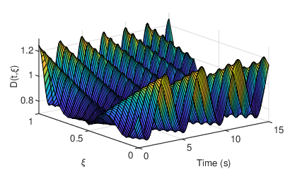
For simulation purposes, we consider the time- and spatially-varying distributed input delay $D(t,\xi)=0.77+0.23|2\xi-1|\left\{1+\sin([3/2+\xi]t+[11\xi-3])\right\}$ for $t\geq 0$ and $\xi\in[0,1]$ ; see Fig. 1. In particular, we have that $|D-D_{0}|\leq 0.23\leq\delta$ . The initial condition is selected as $y_{0}(\xi)=(1-2\xi)/2+20\xi(1-\xi)(\xi-3/5)$ . We set the transition time as $t_{0}=0.2\,\mathrm{s}$ with $\varphi$ linearly increasing from $0$ to $1$ on $[0,t_{0}]$ . The numerical scheme consists of the modal approximation of the reaction-diffusion equation by its $20$ dominant modes. The solution of the the implicit equation (11), used to implement the feedback law (6), is computed based the approximation of the integral appearing in (11) by a Riemann sum. The corresponding simulation results are depicted in Fig 2. They are compliant with the predictions of Theorem 5.

Refer to caption — Figure 1: Time and spatial evolution of the input delay $D(t,\xi)$

5 Conclusion

This paper discussed the problem of in-domain stabilization of a class of infinite-dimensional systems, which operate on a weighted space of square integrable functions over a compact interval, in the presence of an uncertain time- and spatially-varying delay in the distributed actuation. This class includes, for example, reaction-diffusion PDEs. The spatially-varying nature of the delay induces new challenges because it introduces a strong coupling between the space and time variables compared to only time-varying delays configurations. We solved this control design problem by synthesizing a constant-delay predictor feedback on a finite-dimensional truncated model capturing the unstable modes of the original plant. Invoking a small gain argument, we showed that the resulting closed-loop system is exponentially stable provided the fact that the deviations of the delay around its nominal value are small enough. As small gain conditions are, in general, conservative, future works will be devoted to the derivation of relaxed stability conditions.

References

[1] Federico Bribiesca Argomedo, Emmanuel Witrant, and Christophe Prieur. Safety factor profile control in a Tokamak. Springer, 2014.
[2] Zvi Artstein. Linear systems with delayed controls: a reduction. IEEE Transactions on Automatic Control, 27(4):869–879, 1982.
[3] Nikolaos Bekiaris-Liberis and Miroslav Krstic. Robustness of nonlinear predictor feedback laws to time-and state-dependent delay perturbations. Automatica, 49(6):1576–1590, 2013.
[4] Delphine Bresch-Pietri, Christophe Prieur, and Emmanuel Trélat. New formulation of predictors for finite-dimensional linear control systems with input delay. Systems & Control Letters, 113:9–16, 2018.
[5] Haim Brezis. Functional analysis, Sobolev spaces and partial differential equations. Springer Science & Business Media, 2010.
[6] Eduardo Cerpa, Patricio Guzmán, and Alberto Mercado. On the control of the linear Kuramoto-Sivashinsky equation. ESAIM: Control, Optimisation and Calculus of Variations, 23(1):165–194, 2017.
[7] Jean-Michel Coron and Emmanuel Trélat. Global steady-state controllability of one-dimensional semilinear heat equations. SIAM Journal on Control and Optimization, 43(2):549–569, 2004.
[8] Jean-Michel Coron and Emmanuel Trélat. Global steady-state stabilization and controllability of 1D semilinear wave equations. Communications in Contemporary Mathematics, 8(04):535–567, 2006.
[9] Ruth F. Curtain and Hans Zwart. An Introduction to Infinite-Dimensional Linear Systems Theory, volume 21. Springer Science & Business Media, 2012.
[10] Cédric Delattre, Denis Dochain, and Joseph Winkin. Sturm-Liouville systems are Riesz-spectral systems. International Journal of Applied Mathematics and Computer Science, 13:481–484, 2003.
[11] Gerald B Folland. Real analysis: modern techniques and their applications. John Wiley & Sons, 2013.
[12] Emilia Fridman and Yury Orlov. Exponential stability of linear distributed parameter systems with time-varying delays. Automatica, 45(1):194–201, 2009.
[13] Lina Guan, Christophe Prieur, Liguo Zhang, Clementine Prieur, Didier Georges, and Pascal Bellemain. Transport effect of COVID-19 pandemic in France. medRxiv, 2020.
[14] Patricio Guzmán, Swann Marx, and Eduardo Cerpa. Stabilization of the linear Kuramoto-Sivashinsky equation with a delayed boundary control. IFAC PapersOnLine, 52(2):70–75, 2019.
[15] Tomoaki Hashimoto and Miroslav Krstic. Stabilization of reaction diffusion equations with state delay using boundary control input. IEEE Transactions on Automatic Control, 61(12):4041–4047, 2016.
[16] Wen Kang and Emilia Fridman. Boundary control of delayed ODE-heat cascade under actuator saturation. Automatica, 83:252–261, 2017.
[17] Wen Kang and Emilia Fridman. Boundary control of reaction-diffusion equation with state-delay in the presence of saturation. IFAC-PapersOnLine, 50(1):12002–12007, 2017.
[18] Wen Kang and Emilia Fridman. Boundary constrained control of delayed nonlinear Schrödinger equation. IEEE Transactions on Automatic Control, 63(11):3873–3880, 2018.
[19] Iasson Karafyllis and Miroslav Krstic. Delay-robustness of linear predictor feedback without restriction on delay rate. Automatica, 49(6):1761–1767, 2013.
[20] Miroslav Krstic. Lyapunov tools for predictor feedbacks for delay systems: Inverse optimality and robustness to delay mismatch. Automatica, 44(11):2930–2935, 2008.
[21] Miroslav Krstic. Control of an unstable reaction-diffusion PDE with long input delay. Systems & Control Letters, 58(10-11):773–782, 2009.
[22] Hugo Lhachemi and Christophe Prieur. Feedback stabilization of a class of diagonal infinite-dimensional systems with delay boundary control. IEEE Transactions on Automatic Control, 2021, in press.
[23] Hugo Lhachemi, Christophe Prieur, and Robert Shorten. An LMI condition for the robustness of constant-delay linear predictor feedback with respect to uncertain time-varying input delays. Automatica, 109:108551, 2019.
[24] Hugo Lhachemi, Christophe Prieur, and Emmanuel Trélat. PI regulation of a reaction-diffusion equation with delayed boundary control. IEEE Transactions on Automatic Control, 2021, in press.
[25] Hugo Lhachemi and Robert Shorten. Boundary input-to-state stabilization of a damped Euler-Bernoulli beam in the presence of a state-delay. arXiv preprint arXiv:1912.01117, 2019.
[26] Hugo Lhachemi and Robert Shorten. Boundary feedback stabilization of a reaction–diffusion equation with Robin boundary conditions and state-delay. Automatica, 116:108931, 2020.
[27] Hugo Lhachemi, Robert Shorten, and Christophe Prieur. Control law realification for the feedback stabilization of a class of diagonal infinite-dimensional systems with delay boundary control. IEEE Control Systems Letters, 3(4):930–935, 2019.
[28] Hugo Lhachemi, Robert Shorten, and Christophe Prieur. Exponential input-to-state stabilization of a class of diagonal boundary control systems with delay boundary control. Systems & Control Letters, 138:104651, 2020.
[29] Zhao-Yan Li, Bin Zhou, and Zongli Lin. On robustness of predictor feedback control of linear systems with input delays. Automatica, 50(5):1497–1506, 2014.
[30] Bojan Mavkov, Emmanuel Witrant, and Christophe Prieur. Distributed control of coupled inhomogeneous diffusion in tokamak plasmas. IEEE Transactions on Control Systems Technology, 27(1):443–450, 2017.
[31] Serge Nicaise and Cristina Pignotti. Stabilization of the wave equation with boundary or internal distributed delay. Differential and Integral Equations, 21(9-10):935–958, 2008.
[32] Serge Nicaise and Julie Valein. Stabilization of the wave equation on 1-D networks with a delay term in the nodal feedbacks. Networks & Heterogeneous Media, 2(3):425–479, 2007.
[33] Serge Nicaise, Julie Valein, and Emilia Fridman. Stability of the heat and of the wave equations with boundary time-varying delays. Discrete and Continuous Dynamical Systems, 2(3):559, 2009.
[34] Christophe Prieur and Emmanuel Trélat. Feedback stabilization of a 1-D linear reaction–diffusion equation with delay boundary control. IEEE Transactions on Automatic Control, 64(4):1415–1425, 2018.
[35] Jie Qi, Miroslav Krstic, and Shanshan Wang. Stabilization of reaction–diffusions PDE with delayed distributed actuation. Systems & Control Letters, 133:104558, 2019.
[36] Michael Renardy and Robert C Rogers. An introduction to partial differential equations, volume 13. Springer Science & Business Media, 2006.
[37] David L Russell. Controllability and stabilizability theory for linear partial differential equations: recent progress and open questions. SIAM Review, 20(4):639–739, 1978.
[38] D Schley and SA Gourley. Linear stability criteria in a reaction-diffusion equation with spatially inhomogeneous delay. Dynamics and Stability of Systems, 14(1):71–91, 1999.
[39] Anton Selivanov and Emilia Fridman. Predictor-based networked control under uncertain transmission delays. Automatica, 70:101–108, 2016.
[40] Yelena Smagina, Olga Nekhamkina, and Moshe Sheintuch. Stabilization of fronts in a reaction- diffusion system: Application of the Gershgorin theorem. Industrial & engineering chemistry research, 41(8):2023–2032, 2002.
[41] Oren Solomon and Emilia Fridman. Stability and passivity analysis of semilinear diffusion PDEs with time-delays. International Journal of Control, 88(1):180–192, 2015.
[42] Yufang Wang, Kuai Xu, Yun Kang, Haiyan Wang, Feng Wang, and Adrian Avram. Regional influenza prediction with sampling twitter data and pde model. International journal of environmental research and public health, 17(3):678, 2020.

		$\displaystyle\\|z(t-\tau)-z(t-D_{0})\\|$
		$\displaystyle\quad\leq\\|e^{A_{\mathrm{cl}}(D_{0}-\tau)}-I\\|\\|z(t-D_{0})\\|$
		$\displaystyle\quad\phantom{\leq}\,+\left\\|\int_{t-D_{0}}^{t-\tau}e^{A_{\mathrm{cl}}(t-\tau-s)}\Delta(s)\,\mathrm{d}s\right\\|$
		$\displaystyle\quad\leq(e^{\\|A_{\mathrm{cl}}\\|\delta}-1)\\|z(t-D_{0})\\|$
		$\displaystyle\quad\phantom{\leq}\,+M_{\delta}\left\|\int_{t-D_{0}}^{t-\tau}e^{-\sigma(t-\tau-s)}\\|\Delta(s)\\|\,\mathrm{d}s\right\|.$

		$\displaystyle\sup\limits_{s\in[t_{0}+D_{0}+\delta,t]}e^{\kappa s}\\|\Delta(s)\\|$		(18)
		$\displaystyle\quad\leq C_{1}(\delta)\sup\limits_{s\in[t_{0}+\delta,t-D_{0}]}e^{\kappa s}\\|z(s)\\|$
		$\displaystyle\quad\phantom{\leq}\,+C_{2}(\delta)\sup\limits_{s\in[t_{0},t-(D_{0}-\delta)]}e^{\kappa s}\\|\Delta(s)\\|$

	$\displaystyle\\|z(t)\\|$	$\displaystyle\leq C_{4}(\delta)e^{-\kappa t}\\|z(t_{0})\\|$		(21)
		$\displaystyle\phantom{\leq}\,+C_{5}(\delta)e^{-\kappa t}\sup\limits_{s\in[t_{0},t_{0}+D_{0}+\delta]}e^{\kappa s}\\|\Delta(s)\\|.$

	$\displaystyle\\|x(t)\\|$	$\displaystyle\leq\\|z(t)\\|+\int_{t-D_{0}}^{t}e^{\|t-D_{0}-s\|\\|\Lambda\\|}\\|w(s)\\|\,\mathrm{d}s$		(24)
		$\displaystyle\leq C_{8}e^{-\kappa t}\\|x(0)\\|$

	$\displaystyle\sum\limits_{n\geq N+1}\|x_{n}(t)\|^{2}$	$\displaystyle\leq 2e^{-2\gamma t}\sum\limits_{n\geq N+1}\|x_{n}(0)\|^{2}$		(25)
		$\displaystyle\phantom{\leq}\,+\dfrac{2}{\gamma}\int_{0}^{t}e^{-\gamma(t-\tau)}\\|v(\tau)\\|_{\mathcal{H}}^{2}\,\mathrm{d}\tau$

Robustness of constant-delay predictor feedback for in-domain stabilization of reaction-diffusion PDEs with time- and spatially-varying input delaysfootnoteinfo