Incremental Sampling Without Replacement for Sequence Models
Abstract
Sampling is a fundamental technique, and sampling without replacement is often desirable when duplicate samples are not beneficial. Within machine learning, sampling is useful for generating diverse outputs from a trained model. We present an elegant procedure for sampling without replacement from a broad class of randomized programs, including generative neural models that construct outputs sequentially. Our procedure is efficient even for exponentially-large output spaces. Unlike prior work, our approach is incremental, i.e., samples can be drawn one at a time, allowing for increased flexibility. We also present a new estimator for computing expectations from samples drawn without replacement. We show that incremental sampling without replacement is applicable to many domains, e.g., program synthesis and combinatorial optimization.
Keywords:
sampling, without replacement, sequence models, program synthesis, combinatorial optimization1 Introduction
Sampling from programmatically-defined distributions is a fundamental technique. Machine learning problems often involve learning distributions over structured objects such as sentences, images, audio, biological sequences, and source code. These distributions usually factorize into a product of conditional distributions, e.g., the probability of a word given the previous words. Such distributions are naturally represented as programs with sampling operations, which we call randomized programs.
To predict a structured output, traditional search methods like beam search compute a set of predictions that approximately maximize the probability according to a learned model. However, recent work has instead favored sampling from the model, with the goal of obtaining diverse and higher-quality predictions [25, 9, 17, 12, 13, 23]. The same considerations suggest that sampling without replacement could be even more desirable by avoiding duplicate samples, especially in machine learning where the training objective often pushes the output distribution to become extremely peaked.
We present a data structure called UniqueRandomizer for sampling without replacement from randomized programs. The main advantage is that it is incremental, allowing for increased flexibility in stopping conditions for the sampling procedure. For instance, one can draw more samples until a solution is found, or until a sample-based estimate has converged, or enough sample diversity is obtained, and so on. A closely related algorithm for sampling without replacement is Stochastic Beam Search (SBS) [17], based on the Gumbel-top- trick. SBS is mathematically more complex than UniqueRandomizer and does not readily support incrementality, but it has advantages in parallelism and in providing an importance-sampling method for statistical estimation. Fortunately, we are able to present a combined method with both advantages, i.e., the flexibility of incremental sampling and efficiency of batched computations. We also derive an improved estimator that can be used with any method of sampling without replacement.
We experimentally demonstrate that using UniqueRandomizer leads to higher-quality samples in program synthesis and combinatorial optimization. More broadly, a major contribution of this paper is making the case that UniqueRandomizer is a general technique that can be applied to many scenarios.
2 Approach
As a motivating example, consider a program synthesis task: given pseudocode for a short program and some input/output examples, generate the corresponding source code. Suppose that we train a neural sequence-to-sequence model that takes pseudocode as input and generates candidate programs. We would like to sample from the model until we find a program that satisfies the examples.
We do not know upfront how many samples are needed to find a solution, so to minimize computational waste, we want to sample from the model incrementally, one sample at a time until a solution is found. Furthermore, we have no use for duplicate samples because the quality of a sampled program is deterministic. Since we want to trust the trained model’s decisions, we may apply a low temperature when sampling, but this in turn increases the chance of sampling duplicate programs. If we sample without replacement, then we can obtain higher-quality samples while avoiding duplicates altogether. Rejection sampling is a standard approach for this, but can be inefficient for highly skewed distributions, such as what we expect to obtain from a trained model with low sampling temperature. Our approach solves these issues with an augmented trie, described in Section 2.3.
2.1 Problem Formalization
In this section, we formalize the sampling problem that we consider. To unify the broad class of distributions that our method applies to, it is convenient to represent the distribution of interest as a program. Specifically, suppose we have a program that defines a function mapping objects of an arbitrary type to those of type . We further endow with a second argument that acts as a source of randomness—a random choice operation , which samples from the discrete11 1 A discrete randomized program cannot draw a random floating-point number, such as , because this is not a discrete probability distribution. However, the boolean expression Uniform(0, 1) < 0.3 can be rewritten as ([0.3, 0.7]) == 0, which is allowed in . probability distribution , returning a choice with probability , like numpy.random.choice in Python. Except for choices produced by , the program is deterministic. Note that may take other input arguments, and it can use control flow including loops, conditionals, and recursion.
We call any program that has this form a discrete randomized program. This class of programs does not seem to have a standard name in the literature, but it is quite broad, including probabilistic grammars, neural sequence models, and graphical models. Randomized programs are essentially the subset of probabilistic programs [26] without a conditioning operator. An example of a discrete randomized program is shown in Figure 1, which samples from a recurrent neural network. Of course, randomized programs can be more complex than this—for example, the length of the output can be random, such as for programs that sample from a probabilistic context free grammar.
A call to a randomized program defines a distribution over outputs . We assume that the function call terminates with probability 1, although in general this can be tricky to ensure [3]. Our goal is to obtain samples from the distribution incrementally, and without replacement (WOR). Sampling without replacement can be formalized as sampling from a sequence of modified distributions
| (1) |
By sampling incrementally, we mean that samples are drawn one by one with a minimal amount of computation performed for each sample. Given previous samples drawn WOR from , we may easily obtain a new sample drawn from , without slowing down the sampler as increases (as is possible in rejection sampling).
2.2 Sampling WOR with UniqueRandomizer
Our method is able to sample without replacement, even without modifying the program . We introduce a data structure called UniqueRandomizer that defines a drop-in replacement for the random choice operator , which efficiently keeps track of the samples made so far to prevent duplicates. Here, we give an overview of the method, while in the next section we describe the specifics of the UniqueRandomizer data structure and its random choice operator.
To do this, we define two additional concepts. An execution of produces a sequence of calls to . Each such call takes as input a probability distribution and outputs a random choice . We define a trace as the sequence of all random choices produced during a complete execution of . Note that defines a distribution over its traces
| (2) |
UniqueRandomizer samples traces of , incrementally and without replacement, according to .
Sampling WOR from traces yields a sample WOR of program outputs under a particular condition. We say that is trace-injective if necessarily produces different outputs under different traces. This usually occurs when every call to produces a part of the output, such as when sampling from a sequence model. This seems to be the most common situation in machine learning, e.g., the RNN example in Figure 1 is trace-injective. If is trace-injective, then sampling traces WOR is equivalent to sampling outputs WOR (which follows from the change-of-variable rules for discrete distributions), so UniqueRandomizer will produce a sample of outputs without replacement.
Trace-injectivity can be characterized more precisely. First, we define a mapping between traces and program outputs. Every execution of produces a trace and an output let where is the output when executes with trace . Trace-injectivity means that the map is injective. We can extend this map to trace prefixes by defining Then the following theorem says that is trace-injective when every choice contributes to the final output, in a certain sense (proof in Appendix A):
Theorem 1.
is trace-injective for all trace prefixes , the set of possible outputs is partitioned by the next choice , i.e., the set is a partition of
UniqueRandomizer can be used to sample without replacement from a trace-injective discrete randomized program , as shown in Algorithm 1. To obtain samples, we simply run for iterations, providing it with UniqueRandomizer’s RandomChoice function that remembers the sequence of choices that are made by each invocation of , and prevents duplicate traces from being generated. The way in which we do this, as well as the implementation of the functions Initialize, RandomChoice, and ProcessTermination, are described in the next section.
2.3 The UniqueRandomizer Data Structure


Our main idea is to maintain an augmented trie data structure, which we call the UniqueRandomizer, containing the traces that have been generated while executing the program multiple times. Nodes in the trie correspond to trace prefixes seen so far. Each edge represents one element of a trace, i.e., a possible outcome for the next call to . A trie node is a leaf if its trace prefix is actually a full trace, i.e., terminates without further calls to . After terminates, the trie is updated accordingly. Figure 2 shows an example.
Each trie node stores its total unsampled probability mass, denoted . If represents the trace prefix , then equals
| (3) |
We do not compute this sum directly because there will usually be too many traces to enumerate. Instead, we can compute the initial value for a trie node using Equation (2), and then update it incrementally after a trace is sampled (when terminates). This is shown in Algorithm 2.
First, Initialize is called exactly once, before the program is run. When requests a new random choice (RandomChoice in Algorithm 2), we look up the “current” trie node that corresponds to the state of ’s execution. If has not been reached before in a previous execution, we initialize its children. Then, we sample a child of with probability proportional to , update to , and return . When one execution of terminates, we have sampled a full trace , and execute ProcessTermination in Algorithm 2. We mark the corresponding node as a leaf, and we must now update the values. The affected nodes are and all of its ancestors, corresponding to all prefixes of , including itself. For each affected node , we update , where equals before it is updated. Appendix B proves that this scheme results in traces sampled exactly from without replacement.
Finally, it is useful to detect when all possible traces have been sampled. Mathematically, this simply involves checking if the root node has zero unsampled probability mass. In practice however, accumulation of floating-point errors makes this unreliable. Appendix C describes a solution.
2.4 Extensions and Optimizations
Skipping Probability Computations
Notice that the probability distributions computed by and passed to are only needed to compute initial values for the corresponding trie node’s children. Thus, could be modified to only compute probability distributions when needed, depending on whether the current node’s children have already been initialized. This optimization can make sampling with UniqueRandomizer even faster than running in a plain loop (i.e., naïve sampling with replacement), especially when the same initial program states are seen many times while drawing samples.
Incremental Batched Sampling
One downside of UniqueRandomizer is that runs of are difficult to parallelize, since the trie must be updated after each run of before the next run can start. Kool et al. 2019b previously introduced a different approach to sampling without replacement, called Stochastic Beam Search (SBS), which is a modification of beam search using the Gumbel-top- trick to sample beam state expansions WOR. Like normal beam search, SBS allows for parallelization when expanding beam states. Section 3 compares UniqueRandomizer and SBS in detail.
It is actually possible to combine the strengths of UniqueRandomizer and SBS, resulting in a method of incremental batched sampling where each batch allows for parallelization and further batches can be sampled without replacement. Intuitively, one can think of UniqueRandomizer as storing the factorized probability distribution of the next sample, conditioned on the fact that previous samples can no longer be chosen. SBS is run with this probability distribution to select the next batch of samples without replacement, where beam states in SBS correspond to UniqueRandomizer’s trie nodes. After SBS returns a batch of samples, the values in the UniqueRandomizer trie are updated so that the new samples cannot be chosen by later batches.
Locally Modifying Probabilities
By storing more information in the trie, we can enable efficient local updates to the factorized probability distribution, allowing it to change over time in response to new data while still avoiding previously-seen samples. See Appendix D for details.
2.5 Estimating Expectations
Many statistical estimators and learning methods expect i.i.d. samples; is there a way to reweight WOR samples so that they can be used as if they were i.i.d.? Suppose that we have samples drawn without replacement from an arbitrary distribution , perhaps using UniqueRandomizer or some other algorithm, and we wish to estimate the expectation for some function . Estimating an expectation from WOR samples is a fundamental problem in survey statistics [14], but many of these methods do not scale computationally to non-uniform distributions over large outcome spaces.
Kool et al. 2019b present a clever solution to this problem. When asked to produce samples WOR from , SBS actually produces a sequence of samples where the set is the desired WOR sample, and each is an auxiliary variable drawn from a Gumbel distribution [11].22 2 Kool et al. 2019b and Maddison and Tarlow 2017 provide an excellent overview of Gumbels. For more on the Gumbel-top- trick, see Vieira 2014 and Kool et al. 2019b. Kool et al. 2019b use these Gumbels to construct an unbiased estimator of the desired expectation, which we call the threshold Gumbel estimator (TGE):
| (4) |
The “threshold” is the -th largest Gumbel variate obtained during SBS, and , one minus the Gumbel CDF. As usual, it is possible to define a variant that normalizes the weights, introducing bias while often reducing variance [17]:
| (5) |
We derive an equivalent estimator for UniqueRandomizer (which, unlike SBS, does not draw Gumbel variates or produce a threshold). We call this the Hindsight Gumbel Estimator (HGE) because we first draw samples and then draw a set of Gumbel variates conditioned on the samples. After drawing the Gumbels “in hindsight” to obtain , we directly apply Equation (4) or (5). In fact, this technique applies to any method of sampling without replacement. For example, if the probabilities can be enumerated, one can sample an element according to the given probabilities, set that element’s probability to zero, and renormalize the remaining probabilities before drawing the next sample.
To obtain from samples obtained with UniqueRandomizer, we draw a decreasing sequence of Gumbel variates to match the samples (and the remaining unsampled probability mass), as if we had used the Gumbel-top- trick [28] with to sample . In the Gumbel-top- trick, one first draws a Gumbel variate from for every element in some sample space . By selecting the maximum such Gumbels, one actually obtains a WOR sample of elements from from the distribution .
The SBS algorithm implicitly defines a joint distribution . From WOR samples produced by UniqueRandomizer, we sample the hindsight Gumbels from the conditional distribution induced by SBS33 3 Sampling from this conditional distribution is related to the single-sample retrospective Gumbel question considered by Maddison and Tarlow 2017 and Dinh 2016.. To do this, we use a key property of Gumbels: if we draw for every element in some sample space, then .
Because is the first sample, is the maximum Gumbel, so we draw . Then, we draw the subsequent , for , in order: at every iteration, the remaining items have a total probability of , so we draw
| (6) |
where the condition reflects the fact that was sampled before . Appendix B of Kool et al. 2019b describes a numerically stable way to draw from this truncated Gumbel distribution. At the end, we assign and apply Equation (4) or (5). This procedure samples from the same joint distribution over as SBS. Therefore, HGE is equivalent to TGE in the sense that the two estimators have the same distribution, but HGE is more generally applicable to any algorithm for sampling without replacement.
Intuitively, the variance in HGE can be attributed to the samples and the stochastically-chosen . We can reduce variance in the latter case by repeating the “hindsight Gumbel” process to draw multiple (using the same samples), producing multiple HGE estimates. Averaging these gives the Repeated HGE estimate with lower variance.
3 Analysis and Comparison to Related Work
SBS
Stochastic Beam Search [17] is a prior method of sampling WOR from sequence models. It is similar to UniqueRandomizer but has key differences.
First, one main advantage of UniqueRandomizer is that it draws samples incrementally, while SBS returns a fixed-size batch of samples. Thus, UniqueRandomizer allows for increased flexibility in the number of samples drawn, e.g., drawing samples until a solution is found, until a timeout is reached, after sampling a target fraction of the probability space, until reaching enough diversity in samples, or after the Hindsight Gumbel Estimator (Section 2.5) begins to converge. These kinds of stopping criteria would not be possible with SBS44 4 Although beam search and SBS produce batches of distinct samples, drawing multiple batches may lead to duplicates between batches. One also cannot reuse computation performed for one batch without an auxiliary data structure, which is the purpose of the trie in the incremental batched version of UniqueRandomizer.. Because UniqueRandomizer can be used with any arbitrary stopping criterion, it enables sampling-based approaches to be applicable in more scenarios. For example, given a model that generates candidate solutions to a Traveling Salesman Problem instance, SBS could be used to find the best tour among a fixed number of samples, but it would not be able to efficiently find a tour with cost below some threshold. In contrast, UniqueRandomizer is applicable in the latter case due to its incrementality.
Second, like normal beam search, the input to SBS is a next-state function that enumerates the children of a state. For randomized programs , this requires “pausing” and “unpausing” ’s execution. Thus, the state must contain all of the program context (e.g., local variables) necessary to resume execution. While this is easy for a sequence model, it can be challenging for more complex programs. In contrast, UniqueRandomizer can be elegantly implemented as a wrapper on libraries for random number generation, and it is agnostic to the program context that might use.
A third difference is in the number of nodes expanded. When sampling from machine learning models, it is usually expensive to compute the probability distribution over a node’s children required to expand a node. In non-degenerate scenarios, UniqueRandomizer requires fewer expansions than SBS, since UniqueRandomizer only expands the nodes necessary to reach the sampled leaves, while SBS also expands states that later fall off the beam. For example, suppose we sample sequences of length with a vocabulary size . SBS expands exactly beam states. For UniqueRandomizer, the worst case is when all sequences have a different first element, so UniqueRandomizer expands the same number of nodes as SBS. In the best case, only expansions are needed if all sequences differ only at the final position. We also note that the combination of UniqueRandomizer and SBS (incremental batched sampling in Section 2.4) provides smooth intermediate behavior: by sampling batches of size , we reduce the number of expansions with high but obtain better parallelization for low . Setting or reduces to the behavior of UniqueRandomizer or SBS, respectively.
Finally, SBS maintains beam nodes for the current and next time step, where each node stores an arbitrarily-complex intermediate state of . In contrast, UniqueRandomizer stores more nodes (i.e., the entire trie), but each node only stores one value. Using UniqueRandomizer to sample outputs of is at worst a constant factor slower than running in a loop55 5 RandomChoice takes time, but i.i.d. sampling requires time anyway to create the distribution . ProcessTermination takes time where is the leaf depth, which is amortized to an extra time per random choice., but with the optimization in Section 2.4, the UniqueRandomizer approach may actually be faster.
UniqueRandomizer is mathematically simpler than SBS and was developed independently, but we build upon SBS for the incremental batched sampling extension and the Hindsight Gumbel Estimator.
Algorithms for Random Sampling
Matias et al. 2003 describe a dynamic tree data structure to sample from discrete distributions with dynamically changing weights, but this is not naturally adapted to sampling WOR. Various algorithms have been proposed for sampling WOR [31, 30, 7, 8], but generally these algorithms do not consider the case of factorized distributions like (2), and so are inefficient for programs with potentially long traces. The relationship between these methods and the Gumbel-max trick is described by Vieira 2014. The incremental batched version of UniqueRandomizer is related to the top-down Gumbel heap of Maddison et al. 2014. An alternate way of obtaining diverse samples is to explicitly add penalties to beam search to encourage diversity [29, 19]. It is likely possible that UniqueRandomizer can be alternatively implemented using a continuation-passing style and other techniques common in probabilistic programming [10].
4 Experiments
We demonstrate that UniqueRandomizer can lead to improvements in a variety of applications.
4.1 Program Synthesis


We apply UniqueRandomizer to program synthesis as described in the motivating example (Section 2). We use the Search-based Pseudocode to Code (SPoC) dataset [18], which is a collection of 677 problems from programming competitions with 18,356 C++ solution programs written by competitors. Each line of each program has an accompanying human-authored line of pseudocode. Additionally, each problem has corresponding test cases that we can use to verify the correctness of a solution program. The goal is to translate given pseudocode into a code solution for the problem. Compared to natural language translation, the difference is that our “translation” is expected to be syntactically correct code consistent with the test cases, and even a single token error likely means that the translation is incorrect.
We train a Transformer model [27] on the sequence-to-sequence task of generating a line of code given a line of pseudocode. Details are in Appendix E. To sample full programs, we iteratively condition the model on each line of pseudocode and sample one code line for each. Concatenating the code lines produces the full program.
We evaluate on the 3,386 pseudocode prompts in the two test splits of the SPoC dataset, “testp” and “testw,” drawing up to 100 samples for each pseudocode prompt. We compare sampling with replacement (using Monte Carlo i.i.d. sampling) and sampling without replacement (using the batched version of UniqueRandomizer with batch size 10). Each sampled program is checked for correctness using the provided test cases. We use a temperature when sampling with replacement and when sampling without replacement, which we found to be the best among . Note that a low temperature leads to samples for which the model is more confident but also causes more duplicates when sampling with replacement.
For both methods of sampling, we report the number of pseudocode prompts for which a sampled program passes all test cases. Figures 3(a) and 3(b) show that UniqueRandomizer finds solutions with fewer samples than i.i.d. sampling, and succeeds on more prompts overall.
The success rate of our approach is slightly lower than the method in Kulal et al. 2019 which achieves 32.5% success on testp and 51.0% on testw, with a budget of 100 programs and without using compiler diagnostics for error localization. This may be because Kulal et al. 2019 use a more sophisticated model with a copy mechanism and coverage vector, while we simply use a vanilla Transformer. In any case, Kulal et al. 2019 find that using compiler diagnostics increases the success rate by 1.7% on testp and 2.7% on testw, while our approach of sampling WOR improves over i.i.d. sampling by a comparable amount, 2.0% on testp and 2.3% on testw.
Our objective in this experiment was not to surpass the state-of-the-art, but rather to show that using UniqueRandomizer to draw samples without replacement leads to significant improvement over sampling with replacement. Note that beam search and SBS are existing methods of drawing unique samples, but they are not incremental and would be difficult to use in this setting where one does not know upfront how many samples are needed. Additionally, sampling a program takes about 3 times as long as compiling and executing it on the test cases, so drawing fewer samples is important.
Efficiency
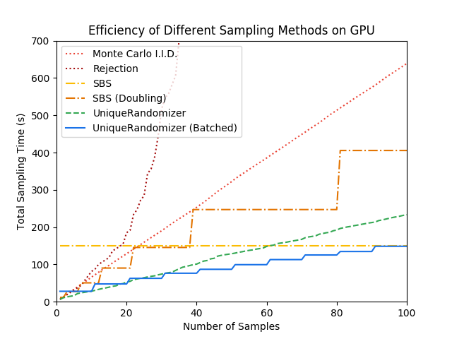
We also examine the efficiency of various sampling methods in Figure 3(c), where we draw 100 samples with a GPU using the same medium-sized pseudocode prompt with 12 lines. We observe that UniqueRandomizer is more than twice as fast as Monte Carlo i.i.d. sampling, explained by the optimization of skipping probability computations (Section 2.4). Further note that UniqueRandomizer produces unique samples, while Monte Carlo i.i.d. sampling does not. Rejection sampling is a naïve method of obtaining unique samples but it is slower than Monte Carlo i.i.d sampling, in fact becoming progressively slower as more samples are drawn. SBS achieves a low time for 100 samples by using batched computations, but all samples are drawn simultaneously, even if a solution is found within the first few samples, and there is no easy way to draw further unique samples if the first 100 samples are insufficient. The batched version of UniqueRandomizer allows for drawing further batches of unique samples, while still taking advantage of batched computation. Thus, if fewer than 100 samples were actually needed, the batched version of UniqueRandomizer would be significantly faster than SBS. We also compare to a naïve way of using SBS “incrementally,” where the batch size doubles on each iteration as and duplicate samples between batches are discarded, but this method is much slower than UniqueRandomizer.
4.2 Traveling Salesman Problem
| Method | Cost | Gap | Duplicates | Cost | Gap | Duplicates | Cost | Gap | Duplicates |
|---|---|---|---|---|---|---|---|---|---|
| Concorde (exact) | 3.8357 | 0% | – | 5.696 | 0% | – | 7.765 | 0% | – |
| AM, with rep. | 3.8397 | 0.105% | 96.8 | 5.735 | 0.69% | 63.6 | 7.979 | 2.77% | 4.2 |
| AM, with rep. | 3.8381 | 0.063% | 1274.5 | 5.724 | 0.49% | 1121.3 | 7.944 | 2.31% | 218.9 |
| AM, w/o rep. | 3.8361 | 0.011% | 0 | 5.726 | 0.53% | 0 | 7.979 | 2.76% | 0 |
| AM, w/o rep. | 3.8358 | 0.002% | 0 | 5.712 | 0.29% | 0 | 7.942 | 2.28% | 0 |
| Method | Cost | Gap | Cost | Gap | Cost | Gap |
|---|---|---|---|---|---|---|
| Concorde (exact) | 3.8357 | 0% | 5.696 | 0% | 7.765 | 0% |
| Bello et al., i.i.d. sampling (*) | – | 5.75 | 0.95% | 8.00 | 3.03% | |
| EAN, i.i.d. sampling (*) | 3.84 | 0.11% | 5.77 | 1.28% | 8.75 | 12.70% |
| AM, i.i.d. sampling | 3.8381 | 0.063% | 5.724 | 0.49% | 7.944 | 2.31% |
| Farthest Insertion, greedy (1 tour) | 3.9262 | 2.358% | 6.011 | 5.53% | 8.354 | 7.59% |
| Farthest Insertion, UniqueRandomizer | 3.8372 | 0.038% | 5.746 | 0.88% | 7.981 | 2.79% |
Sampling without replacement can be used for combinatorial optimization problems, such as the Traveling Salesman Problem (TSP). Several deep learning models for TSP have been proposed [2, 5, 15], where the model outputs candidate tours, and the best tour is chosen among multiple samples drawn from the model. Most recently, the Attention Model by Kool et al. 2018 was shown to be better than the others on randomly-generated TSP instances with , 50, and 100 nodes.
We compare sampling with and without replacement from the Attention Model, using 1280 samples as in Kool et al. 2018, as well as 100 samples. We also record the number of duplicate tours sampled in each setting, which quantifies the amount of computation wasted by i.i.d. sampling (with replacement). Table 1 shows the results on Kool et al. 2018’s dataset. Observe that i.i.d. sampling (used by Kool et al. 2018) results in many duplicate tours, especially on the smaller graphs. The duplicate rate also increases with the number of samples, e.g., from 63.6% duplicate in 100 samples to 87.6% duplicate in 1280 samples for . In contrast, sampling without replacement avoids duplicates altogether, leading to better final costs. For , sampling 100 tours without replacement outperforms sampling 1280 i.i.d. tours with replacement (with optimality gaps of 0.011% and 0.063% respectively).
For this application, incremental sampling with UniqueRandomizer is 5-25% faster than naïve incremental i.i.d. sampling due to the optimization from Section 2.4. In the batched case, sampling without replacement using SBS is about 45-80% slower than batched i.i.d. sampling, but for the smaller graph sizes, the slowdown of SBS is outweighed by the benefit of avoiding duplicate samples.
Farthest Insertion
To demonstrate that UniqueRandomizer is applicable to a wide range of randomized programs, we also consider the farthest insertion heuristic for TSP, which is the best greedy baseline in Kool et al. 2018’s results. This heuristic maintains a cycle for a subset of the nodes, and on each iteration, the node that is farthest from the cycle is inserted into the cycle at the cheapest location (such that the new cycle has minimal cost). We transform the greedy heuristic into a discrete randomized program by relaxing the greedy choice for insertion location. Specifically, if inserting a node at location causes the cycle’s cost to increase by , then we sample an insertion location with probability proportional to where is a temperature hyperparameter. In the limit, corresponds to the greedy heuristic, while corresponds to choosing an insertion location uniformly. We set , , and for , 50, and 100 nodes, respectively. These choices of were obtained from a simple search over the range .
We then use UniqueRandomizer to sample candidate tours without replacement from the modified farthest insertion heuristic. The results are in Table 2. We found that the heuristic approach actually outperforms two of the three learned models included in Kool et al. 2018’s comparison, in fact outperforming all three for .
This result is encouraging given the simplicity of this experiment. We started with a well-known greedy heuristic, and by changing only a few lines of code, we turned it into a randomized program via a straightforward relaxation and used UniqueRandomizer to sample without replacement. By tuning only one hyperparameter (the temperature ), and without any training, we obtained results that are competitive with those of carefully-constructed deep learning models.
4.3 (Repeated) Hindsight Gumbel Estimator
In Section 2.5 we proposed the Hindsight Gumbel Estimator for , the expectation of a function of samples drawn without replacement from a distribution . HGE can be normalized using Equation (5) and/or repeated. Figure 4 shows the performance of the estimators on synthetic data. The Monte Carlo estimate simply averages for i.i.d. sampled with replacement. We see that HGE, normalized and repeated for 10 iterations, has the lowest variance. We chose a heavily-skewed so that sampling with replacement encounters many duplicates, and we enforce a strong correlation between and (or else incorrect estimators might appear to do well). These properties are common when performing estimation in the context of machine learning.

5 Conclusion
We presented UniqueRandomizer, an efficient data structure for incremental sampling without replacement. We also derived the Hindsight Gumbel Estimator, a new estimator for samples drawn without replacement that has lower variance than similar previous estimators. Our experiments show that sampling without replacement leads to significant improvements over i.i.d. sampling in program synthesis and combinatorial optimization. The incremental nature of UniqueRandomizer is especially important in domains like program synthesis where the number of required samples is not known upfront. By eliminating redundant probability computations, UniqueRandomizer also allows for very efficient sampling, and the batched version is even more efficient.
Because UniqueRandomizer is compatible with a broad class of programs, we believe it could be applicable to other problems beyond those explored in this paper. As with our program synthesis and TSP experiments, UniqueRandomizer can be used to sample distinct outputs of a neural model to solve search problems (including constraint satisfaction problems) or obtain diversity in natural language generation [17]. One can also use UniqueRandomizer to perform distinct rollouts in reinforcement learning [16] or Monte Carlo Tree Search [4] to estimate the value of a state with the Hindsight Gumbel Estimator until that estimate converges sufficiently. UniqueRandomizer may also be useful in the context of randomized rounding [24] and probabilistic programming [26].
Our Python implementations of UniqueRandomizer, its batched version, Stochastic Beam Search, and the Hindsight Gumbel Estimator can be found at https://github.com/google-research/unique-randomizer.
Acknowledgments
The authors would like to thank David Dohan, Andreea Gane, David Belanger, Danny Tarlow, and Percy Liang for helpful conversations and explorations.
References
- Applegate et al. [2003] David Applegate, Robert Bixby, Vasek Chvatal, and William Cook. Concorde TSP solver, 2003. URL http://www.math.uwaterloo.ca/tsp/concorde/.
- Bello et al. [2016] Irwan Bello, Hieu Pham, Quoc V Le, Mohammad Norouzi, and Samy Bengio. Neural combinatorial optimization with reinforcement learning. arXiv preprint arXiv:1611.09940, 2016.
- Booth and Thompson [1973] T. L. Booth and R. A. Thompson. Applying probability measures to abstract languages. IEEE Transactions on Computers, C-22(5):442–450, May 1973. ISSN 0018-9340. doi: 10.1109/T-C.1973.223746.
- Browne et al. [2012] Cameron B Browne, Edward Powley, Daniel Whitehouse, Simon M Lucas, Peter I Cowling, Philipp Rohlfshagen, Stephen Tavener, Diego Perez, Spyridon Samothrakis, and Simon Colton. A survey of monte carlo tree search methods. IEEE Transactions on Computational Intelligence and AI in games, 4(1):1–43, 2012.
- Deudon et al. [2018] Michel Deudon, Pierre Cournut, Alexandre Lacoste, Yossiri Adulyasak, and Louis-Martin Rousseau. Learning heuristics for the TSP by policy gradient. In International Conference on the Integration of Constraint Programming, Artificial Intelligence, and Operations Research, pages 170–181. Springer, 2018.
- Dinh [2016] Laurent Dinh. Gumbel-max trick inference. https://laurent-dinh.github.io/2016/11/22/gumbel-max.html, 2016.
- Duffield et al. [2007] Nick Duffield, Carsten Lund, and Mikkel Thorup. Priority sampling for estimation of arbitrary subset sums. J. ACM, 54(6), December 2007. ISSN 0004-5411. doi: 10.1145/1314690.1314696. URL http://doi.acm.org/10.1145/1314690.1314696.
- Efraimidis and Spirakis [2006] Pavlos S Efraimidis and Paul G Spirakis. Weighted random sampling with a reservoir. Information Processing Letters, 97(5):181–185, 2006.
- Fan et al. [2018] Angela Fan, Mike Lewis, and Yann Dauphin. Hierarchical neural story generation. In ACL, 2018.
- Goodman and Stuhlmüller [2014] Noah D Goodman and Andreas Stuhlmüller. The Design and Implementation of Probabilistic Programming Languages. http://dippl.org, 2014. Accessed: 2020-8-13.
- Gumbel [1954] Emil Julius Gumbel. Statistical theory of extreme values and some practical applications: a series of lectures, volume 33. US Government Printing Office, 1954.
- Holtzman et al. [2018] Ari Holtzman, Jan Buys, Maxwell Forbes, Antoine Bosselut, David Golub, and Yejin Choi. Learning to write with cooperative discriminators. In Association for Computational Linguistics, 2018.
- Holtzman et al. [2019] Ari Holtzman, Jan Buys, Maxwell Forbes, and Yejin Choi. The curious case of neural text degeneration. CoRR, abs/1904.09751, 2019. URL http://arxiv.org/abs/1904.09751.
- Horvitz and Thompson [1952] D. G. Horvitz and D. J. Thompson. A generalization of sampling without replacement from a finite universe. Journal of the American Statistical Association, 47(260):663–685, 1952. ISSN 01621459. URL http://www.jstor.org/stable/2280784.
- Kool et al. [2018] Wouter Kool, Herke van Hoof, and Max Welling. Attention, learn to solve routing problems! arXiv preprint arXiv:1803.08475, 2018.
- Kool et al. [2019a] Wouter Kool, Herke van Hoof, and Max Welling. Buy 4 REINFORCE samples, get a baseline for free! ICLR Workshop, 2019a.
- Kool et al. [2019b] Wouter Kool, Herke van Hoof, and Max Welling. Stochastic beams and where to find them: The Gumbel-top-k trick for sampling sequences without replacement. CoRR, abs/1903.06059, 2019b. URL http://arxiv.org/abs/1903.06059.
- Kulal et al. [2019] Sumith Kulal, Panupong Pasupat, Kartik Chandra, Mina Lee, Oded Padon, Alex Aiken, and Percy Liang. Spoc: Search-based pseudocode to code. 2019.
- Li and Jurafsky [2016] Jiwei Li and Dan Jurafsky. Mutual information and diverse decoding improve neural machine translation. CoRR, abs/1601.00372, 2016. URL http://arxiv.org/abs/1601.00372.
- Maddison and Tarlow [2017] Chris J. Maddison and Danny Tarlow. Gumbel machinery. https://cmaddis.github.io/gumbel-machinery, 2017.
- Maddison et al. [2014] Chris J Maddison, Daniel Tarlow, and Tom Minka. A* sampling. In Advances in Neural Information Processing Systems, pages 3086–3094, 2014.
- Matias et al. [2003] Yossi Matias, Jeffrey Scott Vitter, and Wen-Chun Ni. Dynamic generation of discrete random variates. Theory of Computing Systems, 36(4):329–358, Aug 2003. ISSN 1433-0490. doi: 10.1007/s00224-003-1078-6. URL https://doi.org/10.1007/s00224-003-1078-6.
- Radford et al. [2019] Alec Radford, Jeffrey Wu, Rewon Child, David Luan, Dario Amodei, and Ilya Sutskever. Language models are unsupervised multitask learners. Unpublished manuscript, 2019. URL https://d4mucfpksywv.cloudfront.net/better-language-models/language_models_are_unsupervised_multitask_learners.pdf.
- Raghavan and Tompson [1987] Prabhakar Raghavan and Clark D Tompson. Randomized rounding: a technique for provably good algorithms and algorithmic proofs. Combinatorica, 7(4):365–374, 1987.
- Shi et al. [2019] Kensen Shi, Jacob Steinhardt, and Percy Liang. FrAngel: component-based synthesis with control structures. In ACM SIGPLAN Symposium on Principles of Programming Languages (POPL), 2019.
- van de Meent et al. [2018] Jan-Willem van de Meent, Brooks Paige, Hongseok Yang, and Frank Wood. An Introduction to Probabilistic Programming. arXiv e-prints, art. arXiv:1809.10756, Sep 2018.
- Vaswani et al. [2017] Ashish Vaswani, Noam Shazeer, Niki Parmar, Jakob Uszkoreit, Llion Jones, Aidan N Gomez, Łukasz Kaiser, and Illia Polosukhin. Attention is all you need. In Advances in neural information processing systems, pages 5998–6008, 2017.
- Vieira [2014] Tim Vieira. Gumbel-max trick and weighted reservoir sampling. http://timvieira.github.io/blog/post/2014/08/01/gumbel-max-trick-and-weighted-reservoir-sampling/, 2014.
- Vijayakumar et al. [2018] Ashwin K. Vijayakumar, Michael Cogswell, Ramprasaath R. Selvaraju, Qing Sun, Stefan Lee, David J. Crandall, and Dhruv Batra. Diverse beam search for improved description of complex scenes. In National Conference on Artificial Intelligence (AAAI), pages 7371–7379, 2018.
- Vinterbo [2010] Staal A. Vinterbo. Efficient sampling without replacement in Python. https://folk.ntnu.no/staal/programming/algorithms/wrsampling/, 2010.
- Wong and Easton [1980] Chak-Kuen Wong and Malcolm C. Easton. An efficient method for weighted sampling without replacement. SIAM Journal on Computing, 9(1):111–113, 1980.
Appendix A Proof of Theorem 1
Theorem 1.
is trace-injective for all trace prefixes , the set of possible outputs is partitioned by the next choice , i.e., the set is a partition of
Proof.
For any trace prefix , define the collection
First, if is trace-injective, then for any trace prefix , and any , let and . Then there exist traces
and
such that
- (a)
and ,
- (b)
and .
Clearly so because is injective, we have that . Also . This means that is a partition of .
Conversely, assume that is a partition of for any trace prefix . Let
and
be distinct traces. Let be the length of their longest common prefix, so for all , and . By definition,
and
But these two sets are disjoint, because partitions the set . Therefore, , establishing that is injective and that is trace-injective. ∎
Appendix B Proof of Correctness
Theorem 2.
Let be a discrete randomized program that terminates, and let be the probability that runs with trace . Suppose we have already sampled distinct traces . If, at any UniqueRandomizer trie node we move to a child with probability proportional to , then upon reaching a leaf node, the resulting trace is drawn from .
Proof.
Let be any root-to-leaf path, where is the root and is the leaf. Let be the trace corresponding to . According to Equation (3),
We complete the proof by showing that the leaf is reached with the desired probability:
| (7) | ||||
Equality (7) holds because a non-leaf node’s equals the sum of its children’s values. ∎
Appendix C Detecting Exhausted Nodes
We say that a trie node is exhausted if it has zero unsampled probability mass, i.e., all of its probability mass is sampled. Due to floating-point errors, a node’s might not be set to exactly zero after it should be exhausted. We handle this by carefully propagating the information that a given node has zero unsampled probability mass.
When a node is marked as a leaf, we directly assign . Then, when subtracting mass from one of ’s ancestors , we first check if for all children of . If so, we directly set instead of using a subtraction operation. With this approach, a node’s will be exactly after all of its descendent leaves are sampled. Algorithm 3 includes this process, elaborating on the pseudocode in Algorithm 2.
Appendix D Locally Modifying the Factorized Probability Distribution
A slight modification of UniqueRandomizer’s trie allows for efficient local updates to the factorized probability distribution. Instead of storing unsampled probability masses of nodes, the modified trie nodes now store the unsampled fraction of the node’s total probability mass. Edges in the trie now store the initial probability of following that edge from the source node, as given in the probability distribution provided by .
Note that the unsampled probability mass of a node is equal to the product of the edge probabilities from the root to , times the unsampled fraction at . Therefore, by accumulating the product of edge probabilities while walking down the trie, we can compute the unsampled probability mass of nodes, so we can recreate the original UniqueRandomizer behavior with the modified trie.
This decomposition enables local modifications to the factorized probability distribution. More precisely, suppose that a trie node has children, denoted , and initially has outward edge probabilities of . We wish to change these edge probabilities to , so that further samples come from the updated probability distribution and previously-seen samples are still avoided. We do this by updating the trie in the following way. First, we directly replace ’s outward edge probabilities with the desired . Then, we compute the new unsampled fraction at with a weighted average of ’s children:
Finally, we perform a similar update for all of ’s ancestors in upward order (with the root being updated last). After these updates, all values in the trie reflect the new probability distribution.
Appendix E Program Synthesis Experiment Details
For the program synthesis task, we train a Transformer model [27] to translate lines of pseudocode to lines of C++ code. We use the Transformer implementation in the Trax framework66 6 https://github.com/google/trax.. The Transformer uses 2 attention heads, 3 hidden layers, a filter size of 1024, and a hidden dimension size of 512. We train using ADAM with learning rate 0.05 and batch size 512 for 12,000 steps, which is approximately when the models achieve their lowest evaluation loss. We use linear learning rate warmup for the first 1,000 steps. These hyperparameters were chosen from the search space in Table 3, selecting the run with the lowest evaluation loss at the end of training. As in Kulal et al. 2019, we withhold 10% of the training examples as the validation set.
Some of the shorter lines of code in the SPoC dataset have no pseudocode. In some of these instances, we augment the line with pseudocode ourselves. Specifically, if the line is exactly “}” or “};” we provide pseudocode “end”, if the line is exactly “int main() {” we provide pseudocode “main”, and if the line is exactly “return 0;” we provide pseudocode “return”.
| Hyperparameter | Search space | Selected value |
|---|---|---|
| Learning rate | {0.05, 0.075, 0.1, 0.15} | 0.05 |
| Hidden layers | {1, 2, 3} | 3 |
| Hidden dimension size | {512, 1024} | 512 |
| Attention heads | {2, 4} | 2 |
| Filter size | {512, 1024} | 1024 |