Developable cubics in and the Lefschetz locus in Thanks: 2010 Mathematics Subject Classification. 14E05, 16E65 (primary), 14C17 (secondary). Key words and phrases: developable cubics, Artinian Gorenstein algebra, Lefschetz property. The first author was partially supported by CNPq 303599/2016-2 and CAPES-COFECUB 932/19. The third author was partially supported by IMPA summer postdoc 2019/2020 grant.
Abstract.
We provide a classification of developable cubic hypersurfaces in . Using the correspondence between forms of degree on and Artinian Gorenstein -algebras, given by Macaulay-Matlis duality, we describe the locus in corresponding to those algebras which satisfy the Strong Lefschetz property.
1. Introduction
We work over an algebraically closed field of characteristic zero. The projective space over of dimension will be denoted by . In this note we will focus our attention on the classification of developable cubic hypersurfaces on as well as the Artinian Gorenstein algebras defined by them.
An irreducible projective variety is called developable if it has a degenerate Gauss map. Recent progress on the classification problem of de- velopable varieties has been made via the focal locus of the ruling defined by fibers of the Gauss map. For instance, see [AG, MT] for a classification of developable threefolds. In Section 2 we proceed with a careful analysis of the focal locus to provide a finer classification of developable cubic hypersurfaces in . Our first goal is the following result.
Theorem 1.1.
Let be an irreducible cubic hypersurface. Assume that is not a cone. Then is developable if and only if it is projectively equivalent to a linear section of the secant variety of the Veronese surface.
A linear section of the secant variety of the Veronese surface is projectively equivalent to one of the following varieties (see Section 2.4):
- (1)
the secant variety of the rational normal quartic curve;
- (2)
the join of two irreducible conics sharing a single point; this point coincides with the intersection between the planes containing the conics.
- (3)
the dual variety of the scroll surface .
Cases and correspond to cubic hypersurfaces which have nonvanishing Hessian while case yields a cubic with vanishing Hessian.
To each cubic hypersurface above we can associate an Artinian Gorenstein -algebra. More generally, Macaulay-Matlis duality offers a correspondence between forms of degree in variables over , not defining a cone, and standard graded Artinian Gorenstein -algebras of socle degree and codimension . These algebras enjoy nice properties such as Poincaré duality in cohomology theory. We give a precise definition in Section 3.
Given a standard graded Artinian Gorenstein -algebra , AG algebra for short, its Hilbert vector is the vector where . We denote by the space which parametrizes AG algebras with Hilbert vector . It has been extensively studied in [IK]. We are interested in algebras inside which satisfy the Strong Lefschetz property, SLP for short, which means that there exists a linear form such that every multiplication map has maximal rank. This notion was introduced in the commutative algebra setting by R. Stanley and J. Watanabe, see [St, W, HW], and was inspired by the so called hard Lefschetz Theorem on the cohomology of smooth projective complex varieties, see for example [GH]. The Lefschetz properties have attracted a lot of attention over the last years; we refer to [HW] for a survey on the area.
Now we go back to cubic hypersurfaces in which are not cones. They correspond to AG algebras with Hilbert vector , via Macaulay-Matlis duality. We focus on the Strong Lefschetz property of algebras in which come from a developable cubic hypersurface. Algebras associated to cases and above have the SLP, whereas it fails in case . Moreover, by the main result of [MW], any AG algebra with Hilbert vector failing SLP comes from case . Sections 3 and 4 are devoted to the description of the locus of algebras in failing the SLP. The main results of these sections are summarized by the following theorem.
Theorem 1.2.
The space parametrizing AG algebras with Hilbert vector coincides with , where is the space of cubic cones in . Moreover, the following assertions hold:
- (1)
The locus is the image of a projective bundle over by a birational morphism, its dimension is and its degree is .
- (2)
The locus of algebras failing SLP coincides with , where is a rational projective variety of dimension and degree . More precisely, is the image of a projective bundle over the Grassmannian by a birational morphism.
- (3)
The intersection is a divisor in of degree .
We note that the locus of algebras in failing SLP coincides with the locus of algebras with Jordan type , while any other algebra has Jordan type . In particular is the only possible degeneration of the general Jordan type. This phenomenon cannot occur for : in this situation having vanishing Hessian is equivalent to be a cone. Hence, for , any algebra in has the SLP, see [CG].
2. Developable cubics in
2.1. Basic definitions
Given a rational map between projective varieties, its image is the closure of in , where is the maximal domain where is defined. We say that is dominant if it has as image.
Let be a projective subvariety of dimension . Let denote the space of hyperplanes in . We denote by the conormal variety of : this is the closure of the set of pairs such that is a regular point of and contains the tangent space . Let be the image of the projection in the second coordinate. It is the dual variety of . Given a point , we define as the set of hyperplanes passing through it.
Let denote the Grassmannian of -planes in . The Gauss map associates to each regular point the tangent space . We denote by the image of . We say that an irreducible projective variety is developable if
We are particularly interested in the case where is a hypersurface. Assume that it is the zero locus of a non-constant homogenous polynomial in variables. Its polar map is the rational map
where is the partial derivative of with respect to . We denote by the image of the polar map, called polar image of . The restriction of the polar map to is just the Gauss map , and coincides with . We note that since we are working in characteristic zero, the Reflexivity Theorem says that , see [H, p. 208] for an elementary proof.
Let us denote by the Hessian matrix of , namely the matrix of the second derivatives. Its determinant is the Hessian determinant. We shall say that or has vanishing Hessian, if its Hessian determinant is null. Therefore is nondominant if and only if has vanishing Hessian. This is equivalent to say that the derivatives of are algebraically dependent. We summarize the above discussion in the following proposition.
Proposition 2.1.
Let be a hypersurface and its polar image. The following conditions are equivalent.
- (1)
has vanishing Hessian;
- (2)
The partial derivatives of are algebraically dependent;
- (3)
is a proper subvariety of .
The singular locus and the polar image of a hypersurface with vanishing Hessian have a relevant role. The following proposition gives a relation between them. Its proof can be found in the original work of Perazzo, see [P] for the cubic case and [Za2, p. 21] for any degree.
Remark 2.3.
Hypersurfaces with vanishing Hessian are developable. To see this, we assume that has vanishing Hessian. First we note that is a proper subvariety of . In fact if then , but this contradicts Proposition 2.2. The strict inclusions of irreducible varieties imply that , hence is developable.
Given projective subvarieties , we denote by the join between them. It is the closure of the union of lines in joining to . In particular is the secant variety of . A subvariety is a cone if there exists such that . This motivates the definition of the vertex of
Cones are the simplest examples of hypersurfaces with vanishing Hessian. Now we state the following useful proposition the proof of which will be left to the reader.
Proposition 2.4.
Let be a hypersurface. Then the following conditions are equivalent:
- (i)
is a cone;
- (ii)
The partial derivatives of are linearly dependent;
- (iii)
is contained in a hyperplane of ;
- (iv)
is contained in a hyperplane of ;
- (v)
Up to a projective transformation depends on at most variables.
There are many classical examples of varieties with vanishing Hessian which are not cones. The following example appears in the work of Gordan and Noether [GN] and Perazzo [P], called un esempio semplicissimo.
Example 2.5.
Let be the irreducible hypersurface given by
We can check that is not a cone, showing for example the linear independence between the partial derivatives. But since is an algebraic relation among them, has vanishing Hessian.
2.2. Linearity of general fibers and focal locus
In this section we recall some useful results about developable varieties. The main basic fact is that the general fiber of the Gauss map is a union of finitely many linear spaces, see [Se, p. 95]. Actually, it has been proved by Zak that the closure of a general fiber is irreducible. For instance, see [Za1, Theorem 2.3] or [FP, p. 87].
Theorem 2.6 ([Se, Za1]).
Let be an irreducible projective variety. If is developable then the closure of a general fiber of is a linear subspace.
Let be an irreducible projective variety of dimension . When is a hypersurface with vanishing Hessian, the fibers of its polar map share this phenomenon of linearity. We state this result below, the proof can be found in [Za2, Proposition 4.9].
Theorem 2.7 ([Za2]).
Let be a reduced hypersurface with vanishing Hessian. The closure of the fiber of over a general point is a union of finitely many linear subspaces passing through the subspace .
In the next example we illustrate the linearity of fibers of and . Before moving on, we recall the definition of a scroll surface . Let be a line and let be a conic lying on a plane complementary to . Given an isomorphism we let be the union of the lines joining points of to corresponding points of . We note that all the scrolls are projectively equivalent, see for example [H, Example 8.17].
Example 2.8.
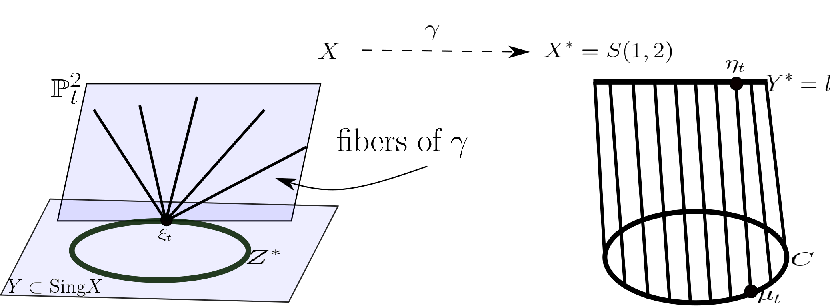
We want to describe the fibers of and where . In particular, we will see in this example that is a scroll surface . See Figure 1.
The singular locus of , with reduced structure, is . Its polar image is the quadratic cone which has as vertex the line . Therefore is a conic contained in . Consider the plane , observe that is a conic and is the join between and .
We denote by , the family of hyperplanes containing and for each let be the corresponding point of . The reader can check that is a union of a plane and , where appears with multiplicity two. A direct calculation shows that for a general point the closure of , , is a line contained in and passing through . In particular, for a general the closure of is a line contained in passing through . Hence is swept out by planes , and fibers of lying in determine a star of lines passing through the point .
Now we prove that is a scroll surface . For a general point , the tangent space contains . Therefore the image of by is . Let be the point corresponding to the unique hyperplane containing and (as , ). Observe that is the line passing through and through . This shows that is a scroll which has as rulings the lines passing through and , .
Let be a developable projective variety. By Theorem 2.6, is ruled by linear subspaces (fibers of the Gauss map) of dimension , where
Let be the open subset where has maximal rank. For each , let be the -dimensional subspace passing through such that is constant along .
We will denote by the closure in of the set . We shall say that is the family of –dimensional subspaces determined by fibers of . Let be a desingularization of and the incidence variety of with natural projection For a general the fiber coincides with the point .
Let be the ramification divisor of and the natural projection on the first coordinate. We can write where the restriction of to any irreducible component of the support of is dominant and of the support of is nondominant. We say that is the horizontal divisor and is the vertical divisor. The direct image by of the horizontal divisor, denoted by , is called the focal locus of .
We note that the restriction of to a general fiber of
is an isomorphism. So the restriction of to defines a divisor in which coincides with the restriction of the focal locus of to . This divisor will be denoted by .
One of the main results concerning developable varieties is the following. For the proof see [IL, Theorem 3.4.2].
Theorem 2.9.
Let be a developable projective variety. If is not a linear subspace, then is singular and its focal locus is contained in . Moreover, for a general belonging to , the restriction of the focal locus to is a divisor in of degree .
2.3. Cubics with vanishing Hessian
Revisiting the work of Perazzo [P], in [GR] the authors provide a classification of cubic hypersurfaces with vanishing Hessian in , for . In this section we rebuild the classification for . This digression will be useful in the next section.
Lemma 2.10.
Let , , be an irreducible cubic hypersurface. Assume there is a component of , with . Then is a linear subspace.
Proof.
Since has degree 3, the secant variety of must be contained in . Hence either , in this case is a linear subspace, or . But the second case cannot occur, because the equality
implies that is a linear subspace, see [Ru, Proposition 1.2.2]. ∎
Remark 2.11.
Here, we note that an irreducible developable cubic surface is a cone. It is well known that a developable surface must be either a cone or the tangent developable to a curve, see [IL, Theorem 3.4.6]. In the last case the curve lies in the singular locus of . Consequently, it follows from Lemma 2.10 that any developable cubic surface in is a cone. Now, let . By taking the smaller linear subspace containing , we can assume that is non-degenerate, and let be a general hyperplane. We will show that . Since is an irreducible non-degenerate curve in of degree , we conclude that , see [H, Proposition 18.9]. If , then is the rational normal curve in and is smooth, but since developable (non-linear) varieties are singular, see [Theorem 2.9], this leads us to a contradiction.
Lemma 2.12.
Let be an irreducible cubic hypersurface. Assume that is not a cone. If contains a linearly embedded then is projectively equivalent to , where .
Proof.
Let us suppose . If is an irreducible polynomial defining one can write , where and are polynomials of degree two. Since the derivatives of must vanish in we can write
where , , are linear forms. If is not a cone, then , and are linearly independent, so there is a projective transformation such that
∎
The following proposition is a classical result of Perazzo [P].
Proposition 2.13.
Let be a cubic hypersurface. Assume that is not a cone. The following conditions are equivalent:
- (i)
has vanishing Hessian;
- (ii)
is projectively equivalent to the scroll surface .
Proof.
First we will show that we can assume irreducible. Suppose that is reducible and is not a cone, then where is a linear form and is homogeneous of degree . In this case its polar map is dominant, as follows by a straightforward computation. This also can be proved (when ) by using the following identity
where denotes the degree of the polar map associated to , see [FM, Corollary 4.3]. Since is a smooth conic, recall that we are assuming is not a cone, then the right side of the identity is positive, which implies that is dominant.
Now we suppose that is irreducible and has vanishing Hessian. By Proposition 2.2, we get . We can assume , otherwise is contained in a hyperplane and Proposition 2.4 ensures that is a cone.
We will show that cannot be a component of . Let us consider the Perazzo map
Since is an irreducible cubic hypersurface, the closure of a general fiber of is a linear space, see [GR, Theorem 2.5]. According with [GR, Proposition 2.16] this implies that lies in the intersection of fibers of . And from [GR, Proposition 2.13] this is equivalent to say that the linear span lies in . Finally, this ensures that if is a component of then , which implies that is a linear subspace. But, in this case must be a cone.
So far we have proved that and cannot be component of . Hence, one may assume that contains a two–dimensional component. It follows from Lemma 2.10 and Lemma 2.12 that is projectively equivalent to , where . This is enough to conclude that , see Example 2.8.
The converse is immediate. Since all scrolls are projectively equivalent, implies that is projectively equivalent to , .
∎
2.4. Sections of the secant variety of the Veronese surface
Linear sections of the secant variety of the Veronese surface are examples of developable cubic hypersurfaces in ; there are three classes of them, up to projectivity, which we now describe.
Let be the three-dimensional vector space . The algebraic group acts on and consequently induces an action of on . We can also consider the action of on the dual space which we see as the space of conics in . The image of the Veronese map
is the Veronese surface. Using coordinates of , the map above can be given by
and if we identify with the projectivization of the space of symmetric matrices, by sending each point of to
then coincides with the locus of matrices of rank one. We note that its secant variety is a cubic hypersurface. Indeed, since any singular matrix can be written as a sum of two rank one matrices then we see that corresponds to the locus of singular matrices.
We now describe and the linear sections of . The preimage by of a hyperplane in is a conic in . The hyperplane is tangent to if and only if the conic is singular, thus the dual variety of is isomorphic to the locus of singular conics in . Since this last coincides with the locus of singular symmetric matrices, we conclude that . A pair of distinct lines in comes from a hyperplane which is tangent to at a single point and whose intersection with yields a pair of conics sharing a single point. A double line in corresponds to a hyperplane which is tangent along a conic.
Since then by biduality we conclude that . In addition, the action of on gives three orbits:
- •
, yielding sections which are transverse to ;
- •
, corresponding to sections which are tangent to at a single point; and
- •
the closed orbit , giving sections which are tangent to along a conic.
Given we set for the corresponding linear section of . From the discussion above, we obtain the following possibilities:
- (1)
if then is a rational normal curve in and is the secant variety of this curve;
- (2)
if then is a union of two irreducible conics and sharing a single point, and is projectively equivalent to the join between them;
- (3)
if then has vanishing Hessian and it is projectively equivalent to , where .
Our next goal is to prove Theorem 1.1, for this purpose we will need some preliminary lemmas.
2.5. Preliminary Lemmas
Let be the family of linear subspaces determined by fibers of the Gauss map . If the dual variety of has dimension two, then is a two–dimensional family of lines. Theorem 2.9 ensures that the restriction of the focal locus of to a general line belonging to is a divisor of degree two in . If has dimension one then is a -dimensional family of -linear subspaces. Applying Theorem 2.9 again, we see that is a divisor of degree one in . The next results will be useful in the proof of Theorem 1.1.
Lemma 2.14.
Let be an irreducible developable cubic hypersurface with nonvanishing Hessian, then has dimension .
Proof.
Since is not a linear subspace, then the dimension of is at least one. We will show that if has dimension then has vanishing Hessian. Assume that . For a general element , is a divisor of degree one in and is contained is . If varies with , then the dimension of the singular set of is at least two. Lemma 2.10 and Lemma 2.12 will imply that has vanishing Hessian. If is a fixed line, say , when varies in then we will show that must be a cone whose vertex contains . This contradicts our hypothesis. Given , let general: for general . We are assuming that the linear subspace passing trough contains . In particular . This implies that . Since is general, we get . This shows that and consequently , which is a contradiction. Therefore has dimension and this concludes the proof. ∎
Lemma 2.15.
Let be an irreducible developable cubic hypersurface such that the support of the focal locus is an irreducible curve. Besides, assume that has dimension two. If the restriction of to a general line belonging to is one point of multiplicity two, then has vanishing Hessian.
Proof.
Let us denote by the support of . Given a general point , let be the cone determined by lines of passing through it. Notice that is a union of these when varies in . The developable hypothesis on implies that these cones are tangent planes to , see [MT, p. 454]. Therefore cannot be a line, otherwise would be a cone.
Since has degree three, the secant variety of , is contained in . Now we analyze the dimension of . If it has dimension three, then and by Terracini Lemma coincides with two distinct points, this contradicts our hypothesis on . If the dimension of equals two, we will show that is contained in the singular set of , which implies that has vanishing Hessian. So, assume that
In this situation, is a linearly embedded , see [Ru, Proposition 1.2.2]. Suppose that is not contained in . Let be a smooth point of and take a tangent line of at passing through . Since belongs to the plane , the tangent space must contain . Thus, is the join between and , that is
Hence, the tangent space of is constant along . But, two lines and , for distinct points and , must intersect at one point. Therefore the tangent space of is constant along . If denotes the tangent space at one general point , then we have for a general point . In this case, we must have and this contradicts our hypothesis .
In order to prove Theorem 1.1 we also need the following result.
Lemma 2.16.
Let be a non-degenerate irreducible curve whose secant variety, , is a cubic hypersurface. Then is a rational normal quartic curve.
Proof.
It is enough to show that . Let be a smooth point, the tangent line at and a linear space skew to , that is, . We consider the projection from which sends to
Note that is the closure of the image of by . We will show that has degree 2 and this implies that has degree 4.
Let be the tangent cone of at . It has as an irreducible component, see [CR, Theorem 3.1]. Since , we get . But cannot be decomposed as product of hyperplanes, otherwise would be degenerate. This shows that and therefore has degree 2. This concludes the proof. ∎
2.6. Proof of Theorem 1.1
Assume that is a developable irreducible cubic hypersurface which is not a cone. If has vanishing Hessian, then Proposition 2.13 yields . Therefore corresponds to a section of which is tangent to along a conic (see Section 2.4).
Suppose that has nonvanishing Hessian. By Lemma 2.14 we get that has dimension two. Thus, is a two–dimensional family of lines. As consequence of Theorem 2.9, the restriction of the focal locus to a general line is a divisor of degree two in .
We first remark that any irreducible component of the support of has dimension one. In fact, if there exists a zero dimensional component, say , then must be a cone because every line must pass through . Besides that, since then from Lemma 2.10 and Lemma 2.12 the existence of a two–dimensional component of will imply that has vanishing Hessian.
The focal locus is the direct image of the horizontal divisor . Recall that the restriction of to gives an isomorphism , for general . The restriction of to is a divisor of degree two which corresponds to , via this isomorphism. Therefore, the support of has at most two irreducible components. A fortiori, the number of irreducible components of is at most two.
We will see that if has two irreducible components then it is a linear section of , with . Suppose is a union of two distinct irreducible curves, say and . Hence must be the join between them, . We first remark that and are plane curves. Indeed, if for example has dimension then and , contradicting our hypothesis on . If and are disjoint, one has (see [H, p. 235])
which means that at least one of these curves is a line and then is a cone. Let us suppose that and are not disjoint and have degree at least two. The two planes containing and must share exactly one point. Otherwise, coincides with the spanned by them. We denote by the intersection point of and . Now we proceed with the same argument of [H, p. 236 Calculation II]. If is a general line, we may describe the intersection by considering a general projection from . Let be the image of by , , and . The points of correspond to the points of distinct of . We note that the intersection outside is transverse, thus
| (1) |
where denotes the intersection multiplicity at . Since and do not share a tangent line, for a general choice of we may assume the same for and . Then is the product of the algebraic multiplicity of and at , say . By the inequality
and from (1) one obtains
Hence is the join between the conics and . The reader can check that is uniquely determined up to a projective transformation. We conclude that with and this concludes the case where has two irreducible components.
Let us assume that is an irreducible curve. If is a general line belonging to , we have two possibilities:
- (1)
;
- (2)
, with .
From Lemma 2.15, the first case cannot happen because we are assuming that has nonvanishing Hessian. If we are in case , then a general line of is secant to the non-degenerate curve and then . By Lemma 2.16, where is a rational normal curve. This corresponds to the case where where . This finishes the proof of Theorem 1.1.
3. The Lefschetz locus in
3.1. Artinian Gorenstein algebras and the Lefschetz property
Let be a graded Artinian -algebra with , we say that is standard graded if and is generated by as algebra. The integer is called the socle degree of . The codimension of coincides with its embedding dimension, that is . If is a standard graded Artinian -algebra, where is an ideal with , then . The Hilbert vector of is , where .
It is a well known fact that is a Gorenstein algebra if and only if and the restrictions of the multiplication in to complementary degrees is a perfect pairing, see [HW, Theorem 2.79]. For standard graded Artinian Gorenstein algebras, the Hilbert vector is symmetric: .
We say that a standard graded Artinian Gorenstein algebra has the Strong Lefschetz Property, or simply has the SLP, if there exists a linear form such that
is an isomorphism for every . In this case is called a strong Lefschetz element.
The following is the model for standard graded Artinian Gorenstein algebras. Let be the polynomial ring in indeterminates and the associated ring of differential operators. Using the classical identification , the ring has a natural structure of module. In fact, differentiation induces a natural action , given by . Let be a homogeneous polynomial of degree . We define the annihilator ideal by
The homogeneous ideal of is also called the Macaulay dual of . We define
One can verify that is a standard graded Artinian Gorenstein -algebra of socle degree , see [MW, Section 1.2]. We assume, without loss of generality, that . This is equivalent to say that the partial derivatives of are linearly independent, which means that is not a cone.
By the theory of inverse systems, we get the following characterization of standard graded Artinian Gorenstein -algebras. It is also called Macaulay-Matlis duality. For a more general discussion of Macaulay-Matlis duality see [HW, Section 2.2], [IK, Section 1.1], [BS, Chapter 10] and [E, Chapter 21].
Theorem 3.1.
( Double annihilator theorem of Macaulay)
Let be an ideal of such that is a standard graded Artinian -algebra of socle degree . Then
is Gorenstein if and only if there exists
such that .
Let be a homogeneous polynomial and the standard graded Artinian Gorenstein algebra associated to .
Let be an ordered -basis of , with . The -th Hessian of is the matrix
Its determinant will be denoted . Note that is the classical Hessian .
The following theorem yields a connection between Lefschetz properties and higher Hessians.
Theorem 3.2.
[MW] Consider , where is a homogeneous polynomial. An element is a strong Lefschetz element of if and only if
for all .
Next we discuss the SLP for standard graded Artinian Gorenstein algebras of socle degree . For such an algebra the Hilbert vector is
We denote by the space of standard graded Artinian Gorenstein algebras of socle degree . By Theorem 3.2, has the SLP if and only if .
By the Gordan-Noether Theorem, if , then if and only if is a cone (see [GN]). Therefore, every standard graded Artinian Gorenstein algebra of socle degree and codimension has the SLP. When has codimension , Proposition 2.13 yields the following result.
Proposition 3.3.
Let be a standard graded Artinian Gorenstein -algebra of Hilbert vector . Assume that does not satisfy the SLP. Then is isomorphic to the following algebra
3.2. Jordan types
Let be a standard graded Artinian -algebra. For consider the map given by . Since , is a nilpotent -linear map. The Jordan decomposition of such a map is given by Jordan blocks with in the diagonal, therefore it induces a partition of which we denote . Indeed, the nilpotent linear map induces a direct sum decomposition of into cyclic -invariant subspaces . The partition is given by the length . Without loss of generality we consider the partition in a non-increasing order.
Given a partition of with , we denote the dual partition obtained from exchanging rows and columns in the Ferrer diagram (diagram of dots). If is another partition of with , we will write and say that is less than in the dominance order if for all we get
If the partition has repeated terms, say with multiplicity respectively, we write
Since is a field of characteristic zero, there is a non empty Zariski open subset of where is constant for , we call it the Jordan type of and we denote it .
The following proposition is a special case of [HW, Proposition 3.64]. It shows that SLP can be described by the Jordan type of .
Proposition 3.4.
Suppose that is a standard graded Artinian -algebra with . Then has the SLP, if and only if, .
Since the generic AG algebra in satisfies the SLP, then the generic Jordan type is .
Example 3.5.
The algebra , , has Hilbert vector and Jordan type
Proposition 3.6.
Let be a standard graded Artinian Gorenstein -algebra of Hilbert vector . If , then has the SLP. If , then the possible Jordan types of are: either if has the SLP or if the SLP fails.
3.3. The Lefschetz locus in
The affine scheme parametrizing AG algebras with Hilbert vector was described by A. Iarrobino and V. Kanev and a great account of their work can be found in [IK]. In their context, stands for the affine cone of the projective variety denoted here. As we have seen, by Macaulay-Matlis duality the scheme can be identified with the parameter space of degree homogeneous polynomials , up to scalars, such that has Hilbert vector . As we noted in the paragraph just before Theorem 3.1, to ensure we assume that , i.e. that in not a cone. Therefore, we have an identification
where and is the parameter space of cubic cones in . In particular
By Theorem 3.2, an AG algebra of socle degree has the SLP if and only if its dual generator satisfies . Proposition 3.6 gives a description of their Jordan types. We summarize this discussion in the following proposition.
Proposition 3.7.
The space can be identified with , where and is the space of cubic cones in . For all the algebras in have the SLP. For , the locus in of algebras satisfying SLP is where can be identified with the locus formed by with vanishing Hessian.
4. Parameter spaces
In this section we find parameter spaces for the locus of cubic cones in , for the locus of cubics with vanishing Hessian and for their intersection; using these descriptions, we compute their dimensions and degrees.
To compute the degree our principal tools are the Segre and Chern classes of a vector bundle. We refer the reader to [F, §3.1, p. 47] or [EH, §10.1 and Ch 5] for a systematic treatment on Segre and Chern classes.
Throughout this section we denote by the vector space . Hence we have: , , .
4.1. Parameter space for cubic cones in
In this section we find a parameter space for cubic cones in and compute its dimension and degree.
A cubic cone in is determined by a point and a cubic hypersurface in the projectivization of the quotient . Consider the tautological sequence on :
| (2) |
The fiber of over can be identified with . Therefore parametrizes cubic hypersurfaces lying in each , where denotes the dual of the vector bundle . Note that is a subbundle of . Thus we have two projections
where is generically injective and is the image of . We have the following result.
Proposition 4.1.
Let be the space of cubic cones in . Then the dimension of is ; its degree is given by the Segre class and is equal to 1365.
Proof.
The dimension can be computed by
and .
This calculation can be generalized to determine the degree of the locus of cones in the space parametrizing hypersurfaces of degree in . Using another characterization for cones, this degree is calculated in [EH, Proposition 7.8, p. 257]. There the authors obtain the following formula for the degree of the locus in of cones of degree :
4.2. Parameter space for cubics with vanishing Hessian
This section is devoted to the description of the parameter space for cubic hypersurfaces with vanishing Hessian in .
Let be the locus of hypersurfaces with vanishing Hessian. As in Proposition 3.7 we denote .
On the other hand, let be the locus formed by such that , where is the ideal of some -plane . It is an irreducible subvariety of , actually we will show below that it is the image by a morphism of a projective bundle over .
Remark 4.2.
We shall find a parameter space for using the above characterization. Let denote the Grassmannian of -planes in . We have the following tautological sequence on :
| (3) |
where is a subbundle of rank and is a bundle of rank .
Consider the multiplication map
It defines a map of vector bundles whose image parametrizes the set of pairs such that .
We claim that the kernel of is exactly . Therefore we have an exact sequence
| (4) |
where .
Let us prove the claim. Consider the following exact diagram
| (5) |
To prove the claim it suffices to prove that is injective. Let be a two-plane, as is a homogeneous variety, we can assume that . Assume lies in the fiber of over , then it can be written as
where are homogeneous polynomials of degree one, . Hence means that lies in the fiber of , i.e. , therefore .
We note that corresponds to a vector bundle over whose projectivization coincides with the incidence variety
Let us denote by and the natural projections. We see that is the image of and is generically injective. Hence one obtains the following result.
Proposition 4.3.
The locus is the birational image of a projective bundle over the Grassmannian . The dimension of is and its degree is , the degree of the Segre class .
Proof.
The dimension can be computed as
Since and the result follows.
We shall write for the hyperplane class of . We have . Using [F, §3.1, p. 47] the degree of is given by
By sequence (4), using the properties of Chern classes [F, §3.2, p. 50], we have
We can compute these characteristic classes using Macaulay2: (see the Scripts in §4.4).
∎
4.3. The locus
In this section we describe the intersection . Let us consider again the tautological sequence on :
Note that corresponds to a vector bundle whose projectivization coincides with the incidence variety
Let and be the natural projections and denote by and their restrictions to .
We will construct a vector bundle over with a birational morphism . Consider the tautological sequence on :
Over we have the following multiplication map:
Its kernel is exactly . This can be proved using the same argument we applied to the multiplication map that appears in Section 4.2. Therefore we have an exact sequence
| (6) |
where . Note that defines a vector bundle whose fiber over a point is equal to the vector space
Let us consider the natural projections and . We see that is generically injective and its image is . Hence one obtains the following result.
Proposition 4.4.
- (1)
is a divisor in .
- (2)
Proof.
The dimension of coincides with
Since and the result follows. In order to compute the degree, write for the hyperplane class of . We have . The degree of is given by
We claim that the following identity occurs in the Chow ring of :
| (7) |
Indeed, exact sequences (2) and (3) yield a map :
which has as zeros. Then it induces a regular section which has as zeros. This proves identity (7) (see [F, ex 3.2.16, p. 61]).
Putting together sequences (4) and (6) we get
Where . Using this, we deduce:
We note that for because is a vector bundle over which has dimension . From this and (7) one obtains that coincides with
where .
In what follows we will omit the pull-back. Computing the Chern classes of a tensor product, we obtain
Observe that
Using this and (4.3), we can reduce the computation of to:
Finally, since and has dimension we have
This number can be computed using Macaulay2/Schubert2, we find . This concludes the proof of proposition. ∎
4.4. Scripts.
loadPackage "Schubert2"
G=flagBundle({1,4})
-- Grassmannian of lines  in 5-space
(S,Q)=G.Bundles
-- names the sub and quotient bundles on G
R=dual (Q)
F=symmetricPower(3,R)
--Computes the classes in Proposition 4.1:
integral(segre(4,F))
loadPackage "Schubert2"
G=flagBundle({3,2})
-- Grassmannian of 3-planes  in 5-space
(S,Q)=G.Bundles
R=dual (Q)
A=symmetricPower(2,R)
B=A^5
C=exteriorPower(2,R)*R
E=B-C
--Computes the classes in Proposition 4.3:
integral(segre(6,E))

--Computes the classes in Proposition 4.4:
integral(3*segre(6,E)+(chern(1,A)+chern(1,Q))*segre(5,E))
Acknowledgments. We wish to thank F. Russo, I. Vainsencher, G. Staglianò and N. Medeiros for pointing out some mistakes in an early draft and for inspiring conversations on the subject.
References
- [AG] M. A. Akivis and V. V. Goldberg. Differential geometry of varieties with degenerate Gauss maps. CMS books in Mathematics (2004).
- [BS] M. P. Brodmann and R. Y. Sharp. Local cohomology: an algebraic introduction with geometric applications. Vol. 136. Cambridge university press (2012).
- [CG] B. Costa and R. Gondim. The Jordan type of graded Artinian Gorenstein algebras. Advances in Applied Mathematics, 111 (2019).
- [CR] C. Ciliberto and F. Russo, Varieties with minimal secant degree and linear systems of maximal dimension on surfaces. Advances in Mathematics, vol. 200, Number 1 (2006), 1–50.
- [E] D. Eisenbud. Commutative algebra: with a view toward algebraic geometry. Vol. 150, Springer Science and Business Media (2013).
- [EH] D. Eisenbud and J. Harris. 3264 and All That: A Second Course in Algebraic Geometry, Cambridge University Press (2016).
- [FM] T. Fassarella and N. Medeiros. On the polar degree of projective hypersurfaces. J. London Math. Soc. (2012) 86 (1): 259–271.
- [FP] G. Fischer and J. Piontkowski. Ruled varieties, an introduction to algebraic differential geometry. Advanced Lectures in Mathematics. Friedr. Vieweg & Sohn, Braunschweig (2001).
- [F] W. Fulton. Intersection Theory. Springer-Verlag. New York. 1985.
- [GN] P. Gordan and M. Noether. Ueber die algebraischen Formen, deren Hesse’sche determinante identisch verschwindet. Math. Ann. 10 (1876), 547–568.
- [GR] R. Gondim and F. Russo. On cubic hypersurfaces with vanishing hessian. Journal of Pure and Applied Algebra. 219 (2015), 779–806.
- [GS] D. Grayson and M. E. Stillman. Macaulay2 version 1.9.2, a software system for research in algebraic geometry. Available at https://faculty.math.illinois.edu/Macaulay2/.
- [GH] P. Griffiths and J. Harris. Principles of algebraic geometry. Wiley, New York (1978).
- [HW] T. Harima, T. Maeno, H. Morita, Y. Numata, A. Wachi and J. Watanabe. The Lefschetz properties. Lecture Notes in Mathematics 2080. Springer, Heidelberg, 2013, xx+250 pp.
- [H] J. Harris. Algebraic geometry, a first course. Springer–Verlag (1992).
- [IK] A. Iarrobino and V. Kanev. Power sums, Gorenstein algebras, and determinantal loci. Springer Science and Business Media (1999).
- [IL] T.A. Ivey and J.M. Landsberg. Cartan for beginners: differential geometry via moving frames and exterior differential systems. Graduate Studies in Mathematics, 61, American Mathematical Society, Providence, RI, xiv+378, (2003).
- [MW] T. Maeno and J. Watanabe. Lefschetz elements of Artinian Gorenstein algebras and Hessians of homogeneous polynomials. Illinois J. Math. 53 (2009), 593–603.
- [MT] E. Mezzetti and O. Tommasi. On projective varieties of dimension n+k covered by k-spaces. Illinois J.Math., 46 nº2, 443–465, (2002).
- [P] U. Perazzo. Sulle varietá cubiche la cui hessiana svanisce identicamente. Giornale di Matematiche (Battaglini), (1900) 38, 337–354.
- [Ru] F. Russo. On the Geometry of some special projective varieties. Lecture Notes of the Unione Matematica Italiana, vol. 18 Springer (2016).
- [Se] C. Segre. Preliminari di una teoria delle varieta luoghi di spazi. Rend. Curc. Mat. Palermo (1) 30 (1910), 87-121 (JFM 41, p. 724.)
- [St] R. Stanley. Weyl groups, the hard Lefschetz theorem, and the Sperner property, SIAM J. Algebraic Discrete Methods 1 (1980), 168–184.
- [W] J. Watanabe. The Dilworth number of Artinian rings and finite posets with rank function. Commutative algebra and combinatorics (Kyoto, 1985), 303?312, Adv. Stud. Pure Math., 11, North-Holland, Amsterdam, 1987.
- [Za1] F. L. Zak. Tangents and secants of algebraic varieties. Transl. Math. Monogr. vol. 127, Amer. Math. Soc., U.S.A. (1993).
- [Za2] F. L. Zak. Determinants of projective varieties and their degrees. Encyclopaedia of Mathematical Sciences , vol. 132, Springer Verlag (2004).