Phonon Transport in Patterned Two-Dimensional Materials from First Principles

Phonon boundary scattering in nanostructures facilitates control over heat flow, enabling several thermal-related applications, including thermoelectrics Vineis et al. 2010; Marconnet et al. 2013, heat guiding and lensing Anufriev et al. 2017. Modeling accurately these systems, however, is particularly challenging because of the nondiffusive nature of heat transport Vega-Flick et al. 2016; in fact, when the characteristic length becomes comparable with the phonon mean free paths (MFPs), ballistic transport may dominate Ziman 2001; Chen 2005 and the Boltzmann transport equation (BTE) must be used Majumdar 1993. A common semplification to the BTE is given by the relaxation time approximation (RTA) where phonon repopulation is neglected (the scattering operator is assumed diagonal). While the RTA has been proven reliable in relevant systems, such as Si Esfarjani et al. 2011, it severely underpredicts the thermal conductivity of several two-dimensional materials, including graphene Fugallo et al. 2014, boron nitride Lindsay and Broido 2011 and molybdenum disulphide Cepellotti et al. 2015. In fact, in these systems the scattering operator has significant off-diagonal components and size effects are dictated by the “generalized” phonon MFPs, significantly larger than the standard MFPs Li et al. 2014. Lastly, the RTA cannot capture phonon hydrodynamic effects and second sound Huberman et al. 2019.

Several models have been developed to compute space-resolved thermal transport beyond the RTA. Cepellotti et al Cepellotti et al. 2015 have applied the concept of relaxons to model heat transport in molybdenum disulfide nanoribbons Cepellotti and Marzari 2017. Landon et al  Landon and Hadjiconstantinou 2014 and Mei et al Mei et al. 2014, solved the space-dependent BTE with the phonon Monte Carlo obtaining good agreements with experiments on graphene nanoribbons (GNRs). Marepalli et al  Marepalli et al. 2019 solved the BTE in GNRs with short widths, using Tersoff interatomic potentials, and taking into account phonon confinement. In  Luo et al. 2019, Luo et al, computed second-sound in GNRs by solving the space-dependent Callaway model Callaway 1959. An analytical approach based on Green’s functions has been reported in Chiloyan et al. 2017, where the non-homogeneous BTE is solved also including arbitrary heat sources. Torres et al Torres et al. 2017 developed the “kinetic-collective” model, which is based on the separate contributions from Normal and Umklapp scattering. More recently, Varnavides et al Varnavides et al. 2019a developed the iterative, space-dependent BTE and applied it to silicon nanoparticles and Si/Ge interfaces, with the perturbation being a constant heat source.

We present a framework to compute the effective thermal conductivity of two-dimensional materials with complex shapes from nano- to macro- scales. Our method combines the space-dependent BTE Varnavides et al. 2019a and the concept of effective phonon temperature Romano and Grossman 2015 to calculate the spatially-resolved thermal flux upon the application of a difference of temperature. Furthermore, we identify the solution to the standard diffusive equation as the first guess to our solver; this choice crucially speeds up convergence, enabling simulations that would be prohibitive otherwise. Special emphasis is given to the energy conservation of the energy operator. We apply our method to the prototypical 2D material graphene with different geometries, including nanoribbons and porous configurations. Due to the generalized phonon MFPs, being tents of micrometers at room temperature, we obtain significant reduction in the thermal conductivity even for patterning with a resolution as coarse as 1 $\mu$m. Lastly, we identify a material with very low thermal conductivity, hence appealing to thermoelectric applications. Since the scattering operator includes also momentum-conserving events, our method naturally includes hydrodynamic transport Cepellotti et al. 2015; Lee et al. 2015.

Steady-state phonon transport is described by the linearized Boltzmann transport equation (BTE) Ziman 2001

where $n_{\mu}(\mathbf{r})$ is the space-dependent non-equilibrium phonon distribution, $\mathbf{v}_{\mu}$ is the group velocity, $\Omega_{\mu\nu}$ is the collision matrix, and $\bar{n}_{\mu}(T)$ is the Bose-Einstein distribution at temperature $T(\mathbf{r})$, given by $\bar{n}_{\mu}(T)=\left[e^{\frac{\hbar\omega_{\mu}}{k_{B}T(\mathbf{r})}}-1\right]^{-1}$, with $\omega_{\mu}$ being the phonon angular frequency. The mode label $\mu$ collectively describes wave vector $\mathbf{q}$ (running up to $N$) and polarization $p$. Equation 1 balances out the change in phonon population due to drift (left hand side) and collisions (right hand side). In passing, we note that since the BTE does not take into account resonances or coherent effects, all the results presented below can be considered object for experimental verification only for feature sizes larger than 100 nm Cahill et al. 2003; Muñoz et al. 2010. Nevertheless, for the sake of completeness we provide data also for smaller dimensions. Furthermore, phonon tunnelling across branches Simoncelli et al. 2019 is neglected and beyond the scope of this work.

Eq. 1 can be simplified if we assume small variation of $T$ with respect to the ambient temperature $T_{0}$, so that the equilibrium term can be Taylor expanded to its first order in $T(\mathbf{r})-T_{0}$, i.e. $\bar{n}_{\mu}(T)=\bar{n}_{\mu}(T_{0})+C_{\mu}\left(\hbar\omega_{\mu}\right)^{-1}\left(T(\mathbf{r})-T_{0}\right)$; the term $C_{\mu}$ is the mode-resolved heat capacity, given by $C_{\mu}=k_{\mathrm{B}}\eta_{\mu}^{2}\left(\sinh{\eta_{\mu}}\right)^{-2}$, where $\eta_{\mu}=\hbar\omega_{\mu}/\left(2k_{\mathrm{B}}T_{0}\right)$.

In the following, for clarity we drop out any space dependence. Conveniently, we define the effective phonon temperature as $T_{\mu}=T_{0}+\hbar\omega_{\mu}C_{\mu}^{-1}\left[n_{\mu}-\bar{n}_{\mu}(T_{0})\right]$. The BTE then becomes

where $W_{\mu\nu}=\Omega_{\mu\nu}\omega_{\mu}C_{\nu}\omega_{\nu}^{-1}V^{-1}N^{-1}$ and $S_{\mu}^{\alpha}=C_{\mu}v_{\mu}^{\alpha}V^{-1}N^{-1}$. In deriving Eq. 2, we have used the normalization factor $V_{n}N$, where $V_{n}$ is the $n$-dimensional volume of the unit-cell of the crystal lattice. We note that the matrix $W_{\mu\nu}$ is symmetric. In fact, the collision operator in Eq. 1 can be rewritten as $\Omega_{\mu\nu}=A_{\mu\nu}/\bar{n}_{\nu}(T_{0})/(\bar{n}_{\nu}(T_{0})+1)$, where $A_{\mu\nu}$ is a symmetric positive semidefinite matrix Fugallo et al. 2013; using the expression for $C_{\nu}$, we have $W_{\mu\nu}=\left(V_{n}Nk_{B}T_{0}^{2}/\hbar^{2}\right)^{-1}A_{\mu\nu}\omega_{\mu}\omega_{\nu}$. The matrix $A_{\mu\nu}$ is energy conserving, i.e. $\sum_{\mu}\omega_{\mu}A_{\mu\nu}=0$ Landon 2014. Furthermore, from $A_{\mu\nu}=A_{\nu\mu}$ it follows that $\sum_{\nu}\omega_{\nu}A_{\mu\nu}=0$; consequently, the sum of each row and column of $W_{\mu\nu}$ is zero. However, in practice, energy conservation is not strictly conserved due to the approximation of the Dirac functions in $A_{\mu\nu}$  Landon and Hadjiconstantinou 2014 (see Appendix A). As reported in Appendix B, we enforce strict energy conservation using the Lagrange multipliers method Landon 2014. In light of this discussion, the right hand side of Eq. 2 simply becomes $\sum_{\nu}W_{\mu\nu}T_{\nu}$. In passing, we note that the left hand side of Eq. 2 can be recast into $\nabla\cdot\mathbf{J}_{\mu}$, where $\mathbf{J}_{\mu}=T_{\mu}\mathbf{S}_{\mu}$ is the mode-resolved thermal flux, normalized by $V_{n}N$. Then, summing both sides over the index $\mu$ we obtain vanishing divergence of the total heat flux, another instance of energy conservation. Conversely, within the relaxation time approximation, $W_{\mu\nu}=\delta_{\mu\nu}C_{\nu}/\tau_{\nu}$, and Eq. 2 is not energy conserving. A common remedy is to define $T$ such that $\sum_{\mu}C_{\mu}/\tau_{\mu}\left(T_{\mu}-T\right)=0$, giving $T=\left[\sum_{\mu}C_{\mu}/\tau_{\mu}\right]^{-1}\sum_{\mu}\left(C_{\mu}/\tau_{\mu}\right)T_{\mu}$ Chiloyan et al. 2017; Romano and Grossman 2015; Hua and Minnich 2014; Carrete et al. 2017; Zhang et al. 2019.

To solve Eq. 2, we decompose the collision matrix into two terms, $W_{\mu\nu}=(V_{n}N)^{-1}C_{\mu}/\tau_{\mu}\delta_{\mu\nu}+W^{\mathrm{od}}_{\mu\nu}$ Ziman 2001; Li et al. 2012; Fugallo et al. 2013; Varnavides et al. 2019b, where $W^{\mathrm{od}}_{\mu\nu}$ is the off-diagonal term. The BTE, then, becomes

where $\mathbf{F}_{\mu}=\mathbf{v}_{\mu}\tau_{\mu}$; similarly to Omini and Sparavigna 1995; Li et al. 2014; Varnavides et al. 2019b, Eq. 3 is solved iteratively. The temperature formulation of the BTE facilitates the connection with Fourier’s law, employed here to compute a first guess to the mode temperatures; that is, $T_{\mu}^{(0)}$ is the result of the standard diffusive heat conduction equation $\nabla^{2}T_{F}=0$. Being mode-independent, the right hand side of Eq. 3 at the zeroeth iteration becomes $-T_{F}\tau_{\mu}/C_{\mu}\sum_{\mu\nu}W^{\mathrm{od}}_{\mu\nu}=T_{F}$. The equation for $T_{\mu}^{(1)}$ then becomes $\mathbf{F}_{\mu}\cdot\nabla T_{\mu}^{(1)}+T_{\mu}^{(1)}=T_{F}$, i.e. a reminiscence of the RTA Romano and Grossman 2015. The choice of $T_{F}$ as a proxy for $T_{\mu}^{(0)}$ and the temperature formulation of the BTE in Eq. 3 are the first results of this paper. In passing, we note that for large structures, Eq. 3 is not guaranteed to converge and a relaxation factor (in our work we use 0.75) must be used Varnavides et al. 2019b; This issue is due the fact that the eignvalues of $W_{\mu\nu}$ are not guaranteed to be smaller than 1 Cepellotti and Marzari 2016.

Equation 3 is performed by the upwind finite volume method Romano and Di Carlo 2011; Murthy et al. 2005, implemented within the OpenBTE framework Romano 2020.

The simulation domain is discretized by a Delaunay mesh bounded by a rectangle of sizes $L_{x}=L$ along $\mathbf{\hat{x}}$ and $L_{y}=L$ along $\mathbf{\hat{y}}$; we assume an applied difference of temperature $\Delta T$ = 1 K along the x-axis (hence we have a hot and cold side). Once Eq. 2 is solved, we define the effective “effective” 2D thermal conductivity as

where the integral runs over either the hot or cold side. As in our case $V_{n}$ has the units of area, the physical units of $\mathbf{J}^{\mathrm{2D}}$ and $\kappa^{\mathrm{2D}}_{\mathrm{eff}}$ are different from the 3D case, and are W$K^{-1}$ and Wm^-1, respectively. This argument is consistent with the “sheet thermal conductance” introduced by Wu et al Wu et al. 2016. In macroscopic 2D materials, i.e. with no size effects, these two quantities are related by the 2D Fourier’s law $\mathbf{J}^{\mathrm{2D}}=-\kappa^{\mathrm{2D}}\nabla T$. The traditional effective thermal conductivity can be obtained by $\kappa_{\mathrm{eff}}=\kappa_{\mathrm{eff}}^{\mathrm{2D}}/h$, where $h$ is an effective thickness. In the following, all the results are presented in terms of $\kappa_{\mathrm{eff}}$.

Bulk related data, such as $A_{\mu\nu}$, group velocities, frequencies, and heat capacities are computed by means of the density functional theory implemented in QUANTUM ESPRESSO Giannozzi et al. 2009, and taken from Chiloyan et al. 2017. The bulk thermal conductivity ($\kappa^{xx}$) is computed within RTA and using the full collision operator (we will refer to this case simply as “Full”), giving $\approx$ 546 Wm^-1k^-1 and 3888 Wm^-1K^-1, respectively, with an effective thickness $h=3.35\AA$. In absence of size effects, the left hand side of Eq. 2 is constant and the bulk thermal conductivity is obtained by multiplying both sides of Eq. 2 by $\mathbf{W}^{\sim 1}$, where $\sim 1$ is the Moore-Penrose inverse, giving $-\sum_{\nu}\mathbf{W}^{\sim 1}_{\mu\nu\beta}S_{\nu}^{\beta}\partial_{\beta}T_{\nu}=T_{\mu}$. The total heat flux, therefore, becomes $J^{\alpha}=-\sum_{\mu\nu}\kappa_{\mu\nu}^{\alpha\beta}\partial_{\beta}T=-\kappa^{\mathrm{2D}}_{\alpha\beta}\partial_{\beta}T$, where

is named the “cross-mode” thermal conductivity; such a quantity can be interpreted as the heat dissipated on mode $\mu$ when a gradient on the mode temperature $T_{\nu}$ is applied. The bulk thermal conductivity is then given compactly by $\kappa_{\alpha\beta}^{\mathrm{2D}}=\braket{S^{\alpha}|W^{\sim 1}|S^{\beta}}$. In passing, we note that within RTA, in Eq. 3 $W^{\mathrm{od}}_{\mu\nu}=0$ Ziman 2001; in this case $\kappa_{\mu\nu}^{\alpha\beta}=(V_{n}N)S_{\mu}^{\alpha}\left(\tau_{\mu}/C_{\mu}\right)S_{\mu}^{\beta}\delta_{\mu\nu}=(V_{n}N)^{-1}C_{\mu}v_{\mu}^{\alpha}v_{\mu}^{\beta}\tau_{\mu}\delta_{\mu\nu}$ recovering kinetic theory.

We first apply our formalism to graphene nanoribbons with infinite lengths and varying width $L$. As shown in the inset of Fig. 1(a), the simulation domain is a square with side $L$ with both periodic boundary conditions and a temperature gradient imposed along the x-axis. This condition is ensured by setting $T_{\mu}^{L}=T_{\mu}^{R}+\Delta T$, where $T_{\mu}^{L(R)}$ is the mode temperature at the left (right) side of the simulation domain. Note that the heat flux is periodic since $\sum_{\mu}\mathbf{\mathbf{S}}_{\mu}\Delta T=0$. Along the y-axis, we assume rough surface, i.e. where phonons lose memory upon scattering and are bounced back diffusively. In practice, we set phonons leaving the pores’ boundary, $T_{B}$, to a weighted average of all the incoming flux Romano and Kolpak 2019, $T_{B}=\sum_{\mu}\alpha_{\mu}T_{\mu}/\sum_{\mu}\alpha_{\mu}$, where $\alpha_{\mu}=C_{\mu}\mathbf{v}_{\mu}\cdot\mathbf{\hat{n}}\mathcal{H}(\mathbf{v}_{\mu}\cdot\mathbf{\hat{n}})$. The term $\mathcal{H}$ is the Heaviside function and $\mathbf{\hat{n}}$ is the normal to the surface. This boundary condition is also applied along any internal surface, such as the pores’ boundary.

Fig. 1(a) shows $\kappa_{\mathrm{eff}}$ for different nanoribbons’ widths. For both RTA and Full cases we observe the ballistic-to-diffusive crossover Bae et al. 2013, i.e. the transition from a width-dependent $\kappa^{\mathrm{eff}}$ to a regime where heat transport depends only on macroscopic geometric effects. For nanoribbons, this limit is the bulk thermal conductivity. In the Full case, the crossover occurs at a threshold, $L_{\mathrm{diff}}$, that is much larger than that for the RTA case. In fact, from Eq. 5 we note that when the full collision operator is used, heat transport in bulk is dictated by the “generalized” phonon MFPs $|\mathbf{G}|=|\sum_{\nu}\mathbf{W}^{\sim 1}_{\mu\nu}\mathbf{S}_{\nu}|$ Fugallo et al. 2014; Li et al. 2014. As shown in Fig. 2(a), the cumulative bulk thermal conductivity distribution versus $|\mathbf{G}|$ spans several micrometers whereas the maximum $|\mathbf{F}|$ of heat-carrying phonons is only a few hundred nanometers. When the off-diagonal terms are related to Normal scattering, i.e. momentum-conserving collisions, this effects can be regarded as phonon hydrodinamic transport Cepellotti and Marzari 2017; Lee et al. 2015. The interaction with boundaries for widths much larger than phonon MFPs reflects also in the heat flux profile, which decreases close to the walls even for L = 10 $\mu$m (see Fig. 1(b)). This trend is in agreement with Montecarlo simulations Landon and Hadjiconstantinou 2014 and consistent with the concepts of friction length applied to molybdenum disulfide nanoribbons Cepellotti et al. 2015; Cepellotti and Marzari 2017.

We investigate thermal transport in porous materials with square pores arranged in a regular lattice. In absence of size effects, $\kappa_{\mathrm{eff}}$ in these systems is solely determined by the porosity, via the Eucken-Garnett formula Nan et al. 1997 $\kappa_{\mathrm{eff}}\approx\kappa_{xx}\frac{1-\varphi}{1-\varphi}$ = 2093 Wm^-1k^-1 (294 Wm^-1k^-1 for RTA). Within RTA, size effects occur when the pore-pore distance becomes comparable to the MFPs Romano and Kolpak 2017; Song and Chen 2004; however, in light of the above discussion, boundary scattering may impact thermal transport even for larger feature sizes, should the off-diagonal terms of the collision operator be significant.

As shown in Fig. 2(a), thermal transport computed with the Full method reaches the diffusive limit around $L$ = 10 $\mu$m, which is consistent with the distribution of the generalized MFPs. For periodicities as large as 1 $\mu$m, which corresponds roughly to pore-pore distance of 435 nm, we obtain roughly a two-fold reduction with respect to the diffusive limit. Another effect of nondiffusive behaviour is given by the pseudotemperature map, shown in Fig. 2(c). In fact, a cut along the applied temperature difference (which is positive) shows a positive gradient in the distance between the pores, clearly violating Fourier’s law. Lastly, the thermal flux, shown in the bottom inset of Fig. 2(d), is pronounced in the space between the pores along the temperature gradient, a signature of ballistic transport. These results, which are consistent with previous literature based on the RTA Duncan et al. 2019; Hao et al. 2009, can be exploited at much larger scales than the phonon MFPs, thanks to the significant off-diagonal term of the scattering operator Fugallo et al. 2014; Cepellotti et al. 2015; as a consequence, low-thermal conductivity materials and high thermal routing capabilities can be achieved via mesoscale patterning.

Similarly to Romano and Grossman 2016, we assess whether non aligned configurations may lead to further thermal conductivity reduction. To this end, we consider disordered porous geometries with porosity $\varphi=0.3$. Each configuration comprises nine pores randomnly distributed in x- and y axes. We choose two periodicities, L = 300 nm and L = 3 $\mu$m, for which the pores size are identical to the aligned cases with L = 100 nm, and L = 1 $\mu$m, respectively. We run 100 simulations for each $L$, finding that disordered configurations may lead to a stronger phonon suppression with respect to the aligned counterpart, as shown in Fig. 2(c). This result is mainly due to the reduction in the view factor, i.e. the possibility of phonons to travel between the hot and cold contact with no scattering with the boundaries. As depicted in the inset of Fig. 3(a), heat flux follows a tortuous path along the applied temperature gradient, as opposed to the aligned configuration whereas phonons mostly travel through direct paths. Interestingly, for the case with L = 3 $\mu$m, there is a larger variation in $\kappa_{\mathrm{eff}}$; this effect is due to the interplay between the wider distribution of feature sizes and the generalized MFP distribution.

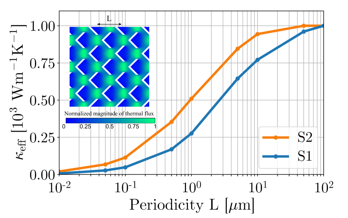
In this last part, we report an example of engineering patterned graphene, where we aim at zeroing the view-factor and ensuring a minimal distance between pores. This requirement rules out solutions with low mechanical stability and vanishing electrical conductivity, an appealing set of properties for thermoelectric applications. We identify the configuration with staggered “less than” signs (S1) as a candidate for this task (see inset of Fig. 3(b)). The chosen porosity is $\varphi$ = 0.12. For comparison, we also examine the aligned configuration with square pores (S2) and same porosity. As we want to focus on size effects, we consider the quantity $\tilde{\kappa}=\kappa_{\mathrm{eff}}/\kappa_{D}$m where $\kappa_{D}$ is the diffusive thermal conductivity. From Fig. 3(b), we see that $\tilde{\kappa}$ of the S1 configuration is consistently smaller than that of the S2 structure, for all $L$; notably, a roughly two-fold difference is obtained for $L$ = 1$\mu$m. Furthermore, from the magnitude of the thermal flux, shown in the inset of Fig. 3(b), we note essentially no flux around the right side of the pore, a signature of phonons shadowing induced by the nanostructure Duncan et al. 2019. This result corroborates the use of convex shapes in minimizing thermal transport in nanostructured materials Gluchko et al. 2019.

We point out that in graphene the electronic thermal conductivity is a significant fraction to the total thermal conductivity, amounting to 10 $\%$ at room temperature Kim et al. 2016. For this reason, topology optimization of 2D materials for heat manipulation should include electronic size effects. While such a combined treatment warrants further research, it is beyond the scope of this work.

In this paper we have introduced a formalism that computes heat transport in arbitrarily patterned 2D materials, solving the linearized phonon BTE beyond the RTA. We first applied the method to graphene nanoribbons, highlighting the role of the generalized MFPs in dictating the ballistic-to-diffusive crossover. Then, we moved to porous graphene, obtaining remarkable thermal transport suppression for mesoscale patterning. Finally, we identify a promising structure with low porosity and low thermal conductivity. Our method opens up possibilities for parameter-free design of 2D systems for thermal routing and energy harvesting applications.
The code will be made available in the next release of OpenBTE Romano 2020.

The collision operator $\Omega$ can be written as

where $A$ is a symmetric and positive semidefinite matrix Fugallo et al. 2014, given by

the term $P^{\mathrm{isot}}$ is the isotope scattering and $P_{\mu\mu^{\prime}l\rightarrow\mu^{\prime\prime}}$ are scattering rates for the coalescent event Fugallo et al. 2014. The latter is given by

where $\Delta_{\mu,\mu^{\prime},-\mu^{\prime\prime}}$ is one when $\mathbf{q}_{\mu}+\mathbf{q}_{\mu^{\prime}}-\mathbf{q}_{\mu^{\prime\prime}}$ is a reciprocal lattice vector and zero otherwise. Lastly, the term $V^{(3)}$ is the third derivative of the energy with respect atomic positions. For details, see Fugallo et al. 2014.

As seen in the main text, the scattering operator needs to satisfy the following conditions

In practice, however, Eq. 9 is not strictly satisfied since the delta functions used in Eq. APPENDIX A: The scattering operator are replaced by Gaussians Landon and Hadjiconstantinou 2014. To ensure strict energy conservation, hence, the non-conserving scattering matrix, denoted by $\tilde{W}_{\mu\nu}$ has to be modified such that $W_{\mu\nu}=\tilde{W}_{\mu\nu}+\beta_{\mu\nu}$ satisfies Eq. 9. In our case, the lack of energy conservation, estimated by $\sum_{\nu}\left|\sum_{\mu}W_{\mu\nu}\right|/\sum_{\nu\mu}\left|W_{\mu\nu}\right|$ Landon 2014, is about 6.5 $\%$. The matrix $\beta_{\mu\nu}$ is computed using the method of the Lagrange multipliers Landon 2014. Specifically, we minimize the function

where $\Delta_{\nu}=\sum_{\mu}\tilde{W}_{\mu\nu}=\sum_{\mu}\tilde{W}_{\nu\mu}$ (where we used the symmetry of W), and $\lambda^{c}_{\nu}$ ($\lambda^{r}_{\mu}$) are the Lagrange multipliers enforcing zero sum for columns (rows). The stationary solution of $F$ is found by solving the following system of equations

which gives $\beta_{mn}=-\left(\lambda^{r}_{n}+\lambda^{c}_{m}\right)/2$, $\sum_{m}\beta_{mn}=-\Delta_{n}$, and $\sum_{n}\beta_{mn}=-\Delta_{m}$. Combining these solutions, we have $N\lambda^{c}_{n}+\sum_{m}\lambda^{r}_{m}=-2\Delta_{n}$ and $N\lambda^{c}_{m}+\sum_{n}\lambda^{r}_{n}=-2\Delta_{m}$. The Lagrange multipliers are obtained by solving the linear system

where $G_{mn}=1/N$ and $\mathbf{I}=\delta_{mn}$. We stress that an energy conserving scattering matrix is paramount to the algorithm detailed in the main text. Nevertheless, after applying the constrain, we note little change in the bulk thermal conductivity, i.e. $\braket{S^{\alpha}|W^{\sim 1}|S^{\beta}}\approx\braket{S^{\alpha}|\tilde{W}^{-1}|S^{\beta}}$.

References

- Vineis et al. (2010) C. J. Vineis, A. Shakouri, A. Majumdar, and M. G. Kanatzidis, Adv. Mater. 22, 3970 (2010).
- Marconnet et al. (2013) A. M. Marconnet, M. Asheghi, and K. E. Goodson, J. Heat Transfer 135, 61601 (2013).
- Anufriev et al. (2017) R. Anufriev, A. Ramiere, J. Maire, and M. Nomura, Nat. Commun. 8, 15505 (2017).
- Vega-Flick et al. (2016) A. Vega-Flick, R. A. Duncan, J. K. Eliason, J. Cuffe, J. A. Johnson, J.-P. Peraud, L. Zeng, Z. Lu, A. A. Maznev, E. N. Wang, and others, AIP Adv. 6, 121903 (2016).
- Ziman (2001) J. M. Ziman, Electrons and Phonons (Oxford University Press, 2001).
- Chen (2005) G. Chen, Nanoscale energy transport and conversion: a parallel treatment of electrons, molecules, phonons, and photons (Oxford University Press, USA, 2005).
- Majumdar (1993) A. Majumdar, J. Heat Transfer 115, 7 (1993).
- Esfarjani et al. (2011) K. Esfarjani, G. Chen, and H. T. Stokes, Phys. Rev. B 84, 85204 (2011).
- Fugallo et al. (2014) G. Fugallo, A. Cepellotti, L. Paulatto, M. Lazzeri, N. Marzari, and F. Mauri, Nano Lett. 14, 6109 (2014).
- Lindsay and Broido (2011) L. Lindsay and D. A. Broido, Phys. Rev. B 84, 155421 (2011).
- Cepellotti et al. (2015) A. Cepellotti, G. Fugallo, L. Paulatto, M. Lazzeri, F. Mauri, and N. Marzari, Nat. Comm. 6, 6400 (2015).
- Li et al. (2014) W. Li, J. Carrete, N. A. Katcho, and N. Mingo, Comput. Phys. Commun. 185, 1747 (2014).
- Huberman et al. (2019) S. Huberman, R. A. Duncan, K. Chen, B. Song, V. Chiloyan, Z. Ding, A. A. Maznev, G. Chen, and K. A. Nelson, Science 364, 375 (2019).
- Cepellotti and Marzari (2017) A. Cepellotti and N. Marzari, Nano Lett 17, 4675 (2017).
- Landon and Hadjiconstantinou (2014) C. D. Landon and N. G. Hadjiconstantinou, J. Appl. Phys. 116, 163502 (2014).
- Mei et al. (2014) S. Mei, L. N. Maurer, Z. Aksamija, and I. Knezevic, J. Appl. Phys. 116, 164307 (2014).
- Marepalli et al. (2019) P. Marepalli, D. Singh, and J. Y. Murthy, J. Appl. Phys. 125, 234302 (2019).
- Luo et al. (2019) X. P. Luo, Y.-Y. Guo, M.-R. Wang, and H.-L. Yi, Phys. Rev. B 100, 155401 (2019).
- Callaway (1959) J. Callaway, Phys. Rev. 113, 1046 (1959).
- Chiloyan et al. (2017) V. Chiloyan, S. Huberman, Z. Ding, J. Mendoza, A. A. Maznev, K. A. Nelson, and G. Chen, arXiv:1711.07151 (2017).
- Torres et al. (2017) P. Torres, A. Torelló, J. Bafaluy, J. Camacho, X. Cartoixà, and F. X. Alvarez, Phys. Rev. B 95, 165407 (2017).
- Varnavides et al. (2019a) G. Varnavides, A. S. Jermyn, P. Anikeeva, and P. Narang, Phys. Rev. B 100, 115402 (2019a).
- Romano and Grossman (2015) G. Romano and J. C. Grossman, J. Heat Transf. 137, 71302 (2015).
- Lee et al. (2015) S. Lee, D. Broido, K. Esfarjani, and G. Chen, Nat. Comm. 6, 6290 (2015).
- Cahill et al. (2003) D. G. Cahill, W. K. Ford, K. E. Goodson, G. D. Mahan, A. Majumdar, H. J. Maris, R. Merlin, and S. R. Phillpot, J. Appl. Phys. 93, 793 (2003).
- Muñoz et al. (2010) E. Muñoz, J. Lu, and B. I. Yakobson, Nano Lett. 10, 1652 (2010).
- Simoncelli et al. (2019) M. Simoncelli, N. Marzari, and F. Mauri, Nat. Phys. 15, 809 (2019).
- Fugallo et al. (2013) G. Fugallo, M. Lazzeri, L. Paulatto, and F. Mauri, Phys. Rev. B 88, 45430 (2013).
- Landon (2014) C. D. Landon, Brigham Young University, Ph.D. thesis (2014).
- Hua and Minnich (2014) C. Hua and A. J. Minnich, Phys. Rev. B 90, 214306 (2014).
- Carrete et al. (2017) J. Carrete, B. Vermeersch, A. Katre, A. van Roekeghem, T. Wang, G. K. Madsen, and N. Mingo, Comput. Phys. Commun. 220, 351 (2017).
- Zhang et al. (2019) C. Zhang, Z. Guo, and S. Chen, Int. J. Heat Mass. Tran. 130, 1366 (2019).
- Li et al. (2012) W. Li, N. Mingo, L. Lindsay, D. A. Broido, D. A. Stewart, and N. A. Katcho, Phys. Rev. B 85, 195436 (2012).
- Varnavides et al. (2019b) G. Varnavides, A. S. Jermyn, P. Anikeeva, and P. Narang, Phys. Rev. B 100, 115402 (2019b).
- Omini and Sparavigna (1995) M. Omini and A. Sparavigna, Physica B 212, 101 (1995).
- Cepellotti and Marzari (2016) A. Cepellotti and N. Marzari, Phys. Rev. X 6, 41013 (2016).
- Romano and Di Carlo (2011) G. Romano and A. Di Carlo, IEEE Trans. Nanotechnol. 10, 1285 (2011).
- Murthy et al. (2005) J. Y. Murthy, S. V. J. Narumanchi, P.-G. Jose’A, T. Wang, C. Ni, and S. R. Mathur, Int. J. Multiscale Com. 3, 5 (2005).
- Romano (2020) G. Romano, “OpenBTE: a solver for the multiscale, space-dependent phonon Boltzmann transport equation,” (2020).
- Wu et al. (2016) X. Wu, V. Varshney, J. Lee, Y. Pang, A. K. Roy, and T. Luo, Chem. Phys. Lett. 669, 233 (2016).
- Giannozzi et al. (2009) P. Giannozzi, S. Baroni, N. Bonini, M. Calandra, R. Car, C. Cavazzoni, D. Ceresoli, G. L. Chiarotti, M. Cococcioni, I. Dabo, A. Dal Corso, S. de Gironcoli, S. Fabris, G. Fratesi, R. Gebauer, U. Gerstmann, C. Gougoussis, A. Kokalj, M. Lazzeri, L. Martin-Samos, N. Marzari, F. Mauri, R. Mazzarello, S. Paolini, A. Pasquarello, L. Paulatto, C. Sbraccia, S. Scandolo, G. Sclauzero, A. P. Seitsonen, A. Smogunov, P. Umari, and R. M. Wentzcovitch, J. Phys. Condens. Matter 21, 395502 (2009).
- Romano and Kolpak (2019) G. Romano and A. M. Kolpak, J. Heat Transfer 141, 12401 (2019).
- Bae et al. (2013) M. H. Bae, Z. Li, Z. Aksamija, P. N. Martin, F. Xiong, Z. Y. Ong, I. Knezevic, and E. Pop, Nat. Comm. 4, 1734 (2013).
- Nan et al. (1997) C.-W. Nan, R. Birringer, D. R. Clarke, and H. Gleiter, J. Appl. Phys. 81, 6692 (1997).
- Romano and Kolpak (2017) G. Romano and A. M. Kolpak, Sci. Rep. 7, 44379 (2017).
- Song and Chen (2004) D. Song and G. Chen, Appl. Phys. Lett. 84, 687 (2004).
- Duncan et al. (2019) R. A. Duncan, G. Romano, M. Sledzinska, A. A. Maznev, J.-P. M. Peraud, O. Hellman, C. M. S. Torres, and K. A. Nelson, arXiv:1912.06211 (2019).
- Hao et al. (2009) Q. Hao, G. Chen, and M.-S. Jeng, J. Appl. Phys. 106, 114321 (2009).
- Romano and Grossman (2016) G. Romano and J. C. Grossman, Phys. Rev. B 1, 3434 (2016).
- Gluchko et al. (2019) S. Gluchko, R. Anufriev, R. Yanagisawa, S. Volz, and M. Nomura, Appl. Phys. Lett. 114, 23102 (2019).
- Kim et al. (2016) T. Y. Kim, C.-H. Park, and N. Marzari, Nano Lett. 16, 2439 (2016).