Magic squares of subtraction of Adam Adamandy Kochański
Abstract
The problem of the construction of magic squares occupied many mathematicians of the 17th century. The Polish Jesuit and polymath Adam Adamandy Kochański studied this subject too, and in 1686 he published a paper in Acta Eruditorum titled “Considerationes quaedam circa Quadrata et Cubos Magicos”. In that paper he proposed a novel type of magic square, where in every row, column and diagonal, if the entries are sorted in decreasing order, the difference between the sum of entries with odd indices and those with even indices is constant. He called them quadrata subtractionis, meaning squares of subtraction. He gave examples of such squares of orders 4 and 5, and challenged readers to produce an example of square of order 6. We discuss the likely method which he used to produce squares of order 5, and show that it can be generalized to arbitrary odd orders. We also show how to construct doubly-even squares. At the end, we show an example of a square of order 6, sought by Kochański, and discuss the enumeration of squares of subtraction.
1 Introduction
Contributions of Jesuits to science and mathematics have attracted considerable attention in recent years (Feingold 2013; O’Malley et al 2016). It is now well documented that the Society of Jesus played an especially important role in the intellectual life of Polish–Lithuanian Commonwealth (Stasiewicz-Jasiukowa 2004), producing a number of notable writers, preachers, theologians, missionaries, and scientists. The Polish Jesuit Adam Adamandy Kochański (1631–1700) was one of such remarkable individuals. He pursued problems in a multitude of diverse fields, including philosophy, mathematics, astronomy, philology, design and construction of mechanical clocks and computing devices, and many others. He published relatively little, and his published works remain rather unknown today, even among historians of mathematics and science. In recent years, however, his accomplishments seem to have attracted some more interest, in large part due to the efforts of B. Lisiak SJ, who reprinted all the published works of Kochański 2003a; Kochański 2003b; Kochański 2003c and who authored a comprehensive account of Kochański’s life and work (Lisiak 2005). Moreover, B. Lisiak SJ and L. Grzebień SJ gathered and published all the surviving letters of Kochański, including correspondence with Gottfried Leibniz, Athanasius Kircher SJ, Johannes Hevelius, Gottfried Kirch, and many other luminaries of the 17th century (Lisiak and Grzebień 2005).
The most important and original mathematical works of Kochański appeared in Acta Eruditorum between 1682 and 1696. Among those, three are particularly interesting, namely papers published in Acta in Kochański 1682, Kochański 1685, and Kochański 1686 all three reprinted in Kochański 2003a, English translation in Fukś 2015. The 1685 paper, Observationes cyclometricae, is relatively well-known and is often considered to be the most interesting one. It proposes for the rectification of the circle an approximate procedure which received some attention from both contemporaries of Kochański and historians of mathematics (Montucla 1754; Cantor 1880; Günther et al 1921). What is generally less known, however, is that the same paper included an interesting sequence of rational approximations of , somewhat similar to continued fractions. Detailed discussion of this sequence and its properties can be found in a recent article (Fukś 2012), so we will not consider it here. We will only mention that the sequence of integers on which the aforementioned approximation of is based is now included in the Online Encyclopedia of Integer Sequences as A191642 (OEIS Foundation Inc. 2015). I proposed to call it Kochański’s sequence.
The subject of this note is the 1686 paper, Considerationes quaedam circa Quadrata & Cubos Magicos. This work, like all of Kochański’s other papers, touches upon more than one subject. In the first part, “classical” magic squares are discussed, and Kochański presents some previously unknown magic squares using the method of their construction developed by A. Kircher. The second part is more original and interesting, because Kochański introduces there a new type of magic square, to be called quadrata subtractionis or squares of subtraction. An square of subtraction is an arrangement of consecutive integers from 1 to in such a way that in every row, column and diagonal, if the entries are sorted in decreasing order, the difference between the sum of entries with odd indices and the sum of entries with even indices is constant. Kochański gives examples of and squares of subtraction, and then challenges fellow mathematicians to produce an example of a square of order 6. To my knowledge, nobody has ever taken this challenge, and nobody has ever studied magic squares of subtraction in the 330 years following the publication of Considerationes. The only author mentioning magic squares of subtraction in a published work is Z. Pawlikowska (Pawlikowska 1969), who briefly discussed them in a paper describing the mathematical works of Kochański and who guessed the most likely method used by him to produce squares of order 5.
The purpose of this article, therefore, is to bring magic squares of subtraction back to life, with the hope of stimulating others to study their properties and methods of construction. We will take a closer look at the examples supplied by Kochański and present the general method of construction of squares of odd order and doubly-even order, based on these examples. We will also give an example of an square, which he requested, and discuss the enumeration of squares of subtraction.
2 Notation and examples
Kochański defines squares of subtraction as arrangements of the consecutive integers which have the same residuum in rows, columns, and diagonals. His definition of “residuum” is as follows.
In his Quadratis Subtractione tractandis ita proceditur. Numerus in assumpta Columna, Trabe, vel Diagono minimus, subducendus est a proxime majore, residuum majoris hujus detrahatur a proxime consequente, atque ita porro : ultimum enim residuum est illud universale […].
In these Squares produced by Subtraction one proceeds as follows. The smallest number in a selected Column, Row, or Diagonal is subtracted from the next-largest number, the difference is subtracted form the subsequent larger number, and so on: the final result is the universal number […].
This means, for example, that if numbers in a given row, column or diagonal of a square , sorted in decreasing order, are , then the aforementioned residuum is
Obviously, this can be written in a more convenient way, without nested parentheses. Let us, therefore, define the residuum of a vector using modern notation. First, we sort the vector in decreasing order, obtaining such that ; then the residuum of is defined as
| (1) |
A Magic square of subtraction is an arrangement of numbers in a square array such that all rows, columns, and both diagonals have the same residuum. If entries of the array belong to the set , then the magic square of subtraction will be called normal. In what follows we will consider only normal squares (unless indicated otherwise), so we will omit the designation “normal” and we will refer to them simply as squares of subtraction. The number will be called the order of the square of subtraction. Figure 1 shows an example of a square of subtraction of order 4 with residuum equal to 8.
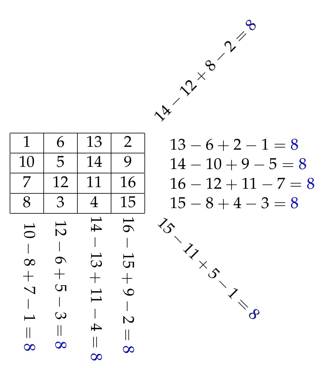
This is actually one of the squares given by Kochański. In the original paper he gave examples of seven other squares of subtraction, of orders 4 and 5, as shown in Figure 2.

It is worth noticing that the smallest order he considered is 4, and that he does not mention any smaller orders. He was likely aware that squares of order 2 and 3 do not exist, and this is not too hard to prove.
3 Formal construction for odd
We will start with odd-order squares, as these are easier to construct. Kochański gives examples of squares of order 5, and this is indeed the smallest possible odd order. The first of these, shown in Figure 2e, is reproduced again in Figure 3, as the framed square. As observed by Pawlikowska 1969, it can be constructed by writing consecutive numbers from 1 to 25 along diagonal lines of length 5, one below the other, with alternating direction. Afterwards, one needs to relocate the numbers which are outside the framed square to its interior, by “wrapping” them back to the square (boldface numbers in Figure 3 are those which have been relocated).


How did Kochański discover this method of construction? From his surviving letters we know that he was familiar with works of Athanasius Kircher SJ, whom he greatly esteemed and with whom he maintained correspondence (Lisiak and Grzebień 2005; Lisiak 2005). In Kircher’s book Arithmologia (Kircher 1665), a method of construction of magic squares of summation is discussed, here reproduced in Figure 4. In this method, we write consecutive integers along diagonal lines, one below the other, but maintaining the same direction. Numbers which fall outside of the square are relocated to the interior of the square. This method has been originally proposed by Claude Gaspard Bachet de Méziriac (Bachet 1624), but since Kochański does not mention Bachet’s name in Considerationes, it seems likely that he learned about it from Kircher (Kircher’s name is explicitly listed in the first paragraph of Considerationes as one of the “ingenious men” who have studied magic squares).
Kochański noticed that by reversing the order in which we write numbers on each diagonal in Kircher’s example, instead of a magic square of summation we obtain a square of subtraction. He did not prove this fact, but merely produced examples. We will now show that this method indeed produces the desired magic squares of subtraction, and that it can be generalized to any odd order . To simplify notation, we will define
| (2) |
Note that if then . This will be used to bring indices of matrices back to the range .
Proposition 1
Let be an odd integer, , , and let
| (3) |
Then the matrix
| (4) |
is a magic square of subtraction of order with residuum .
We will be using Figure 3 to illustrate the proof. Let us first explain where the formulae in eqs. (3) and (4) come from. Note that the magic square of order 5 shown in Figure 3 has been obtained by rotating the matrix
| (5) |
by 45 degrees counterclockwise. The function defined in the proposition is simply the indexing function used to construct , so that . After is rotated, one needs to “squeeze” all entries of this matrix into a square box , shown in Figure 3. “Squeezing” is achieved by relocating all entries which are outside the box to the inside of the box, by bringing their indices to the range with operator. This simply means that each entry located outside the box at is relocated to . The result is the matrix ,
| (6) |
which is the desired magic square of subtraction. The rotation by 45 degrees around the origin can be described algebraically as the transformation , and we need to add to the second index to bring the origin of coordinate system to the right location, thus
| (7) |
Note that the above works only for entries which ended up inside the box, not needing relocation. These happen to be entries for which are both odd or both even. The remaining entries must be relocated, and this is achieved by combined translation and use of the operator , resulting in the second line of eq. (4).

From Figure 3, one can see that the third row of is the diagonal of . Other rows of can be constructed from numbers lying on two diagonal segments of , as illustrated in Figure 5.
This can be easily generalized to arbitrary . For convenience, we will introduce index labeling rows of , such that the actual row number is equal . The middle row of will then always correspond to . The set
| (8) |
composed of two diagonal lines of , contains all entries of the row of . Note that the second component of the above set is empty when , as in this case we only need one diagonal line (the main diagonal).
It is important to notice that the elements of the set are already sorted in descending order, thus we can easily compute its residuum,
| (9) |
Using the definition of (eq. 3) and the fact that is odd, one can easily compute the above sums, obtaining
| (10) |
This means that the residua of all rows of are the same and equal to .
Exactly the same observations can be made for columns of . We label them with the integer , so that the actual column number is . Then all the entries of the column of are contained in the set
| (11) |
As before, the above set is already sorted in descending order, thus
| (12) |
Computing the sums we obtain
| (13) |
confirming that the residuum is the same for every column of .
What is now left is checking the diagonals of . The main diagonal of corresponds to the middle column of , or -th column, . It is sorted in increasing order, thus
| (14) |
The antidiagonal of corresponds to the -th column of , and it is sorted in decreasing order, thus
| (15) |
Both sums in eq. (14) and (15) can be easily computed. They are both equal to , thus is indeed a magic square of subtraction. □
Proposition 1 produces, for , the square shown in Figure 2e. How did Kochański obtain the remaining three squares of order 5, shown in Figures 2f,g and h? He does not explain it in the paper, but it is rather easy to guess, following observations made by Pawlikowska 1969.
Keeping the notation used in the proof of Proposition 1, let us recall that the magic square is obtained by rotating the initial matrix and then relocating outside entries to the interior of the square. Obviously, if is transposed before rotation and relocation, the resulting square will still be magic. Transposition of , therefore, does not affect the magic property. One can also show that any permutation of columns of which keeps the middle column in the same place, performed before the rotation and relocation, preserves the magic property of the resulting square (recall that the middle column of becomes the diagonal of , so it cannot be moved). The same applies to any permutation of rows of keeping the middle row in the same place.
The remaining three 5th order squares of Figure 2 can be obtained if certain operations of the aforementioned type are applied to rows and columns of matrix of eq. (5) before it is rotated. These are shown below.
- •
For the square shown in Figure 2f: transpose , then apply the permutation to the rows of and the permutation to its columns;
- •
For the square shown in Figure 2g: apply the permutation to the rows of and the permutation to its columns;
- •
For the square shown in Figure 2h: apply the same permutation to both the rows and columns of .
The above operations will produce three matrices,
By rotating each one of them and relocating outside entries to the interior we obtain the magic squares of subtraction shown respectively in Figures 2f, 2g, and 2h.
Obviously, since Proposition 1 is valid for any odd , we can use it to construct squares of subtraction of higher orders. Figure 6 show squares of subtraction of order 7 and 9 obtained by this method.
4 Even order
Just as in the case of magic squares of summation, magic squares of subtraction of even order are more difficult to construct. Kochański gave four examples of squares of order 4, the smallest order for which magic squares of subtraction exist, and these are shown in Figures 2a–d. He did not explain how they were constructed. Close inspection of them reveals certain regularities in the arrangement of numbers, and from this one can guess how the construction probably proceeded.
Most likely, his first observation was that that the arrangement of odd and even numbers must follow some pattern reflecting constrains required for the square to be magic. The simplest of such patterns is shown below.
It satisfies the obvious requirement that the residua of all rows, columns and diagonals must have the same parity, and that the total number of odd entries must be the same as the total number of even entries. He then probably proceeded, by trial and error, to fill this pattern with consecutive odd and even integers, and one of the most natural ways to do this would be to follow a “zigzag” path. Such a path does not need to start inside the square, just as in the case of squares of order 5. After some tinkering with such paths, one discovers that the placement of odd and even numbers shown in Figure 7 fits the bill.
1 6 13 2 10 5 14 9 7 12 11 16 8 3 4 15
This requires, as in the case of order 5 square, the relocation of numbers which are outside the square to its interior, using “periodic boundary conditions”, that is, left-right and bottom-top wrapping. One thus discovers the square shown in Figure 2a.
The square of Figure 2b can be produced by applying to the first square the transformation shown schematically in Figure 8.
By direct verification one can check that this indeed produces a magic square of subtraction.
Finally, if we apply to both rows and columns of the squares shown in Figures 2a and 2b the permutation , we will obtain the remaining two squares shown Figures 2c and 2d. Application of the same permutation to both rows and columns preserves the magic property, so we are guaranteed that these are magic squares of subtraction too.
As clever as the above constructions are, they do not seem to be amenable to a generalization to higher orders. However, Kochański claims that he found a general method of construction of doubly-even squares, of course without revealing any details. In spite of the lack of evidence, one might speculate that this general method possibly exploited the existence of squares of order 4 to build larger squares of doubly-even orders. A similar method exists for squares of summation, and is sometimes known as the method of composite squares. This is a very obvious construction, so it seems probable that Kochański was aware of it. We will now show how this can be done.
Let us assume that , . The following proposition constructs magic square of subtraction of order if a known square of order 4 is provided.
Proposition 2
Let be a magic square of subtraction of order 4, be a matrix with all entries equal to 1, and let be a block matrix with entries . Then is a magic square of subtraction of order .
Matrix is simply a block matrix with entries consisting of sums of and matrices , added in consecutive rows in increasing order. For example, for , it is given by
| (16) |
Note that each matrix is a magic square of subtraction, regardless of , and its residuum is the same as the residuum of .
Consider now, for example, the first row of , which consists of the first row of followed by the first row of and then by the first row of , which we will symbolically write as
| (17) |
Note that every entry of is smaller than every entry of , and every entry of is smaller than every entry of . For this reason,
| (18) | |||
| (19) |
Exactly the same relationship holds for every row and column of , as well as for both diagonals, for the same reason as above. Obviously, this observation also easily generalizes to arbitrary , when the residuum of every row, column and both diagonals of would be equal to , proving that is indeed a magic square of subtraction.
For , an example of construction of a square of order 8 using this method is shown below.
This example uses as one of the squares of order constructed by Kochański, with residuum 8. The residuum of the resulting square is equal to .
What remains is the case of singly-even squares, of order , . Kochański apparently tried to construct the smallest order square of subtraction of this type, for , but he failed. For this reason, at the end of his paper, he challenged fellow mathematicians to find the square of order 6:
PROBLEMA I. In Quadrato Senarii, cellulas 36 complectente, numeros progressionis Arithmeticae, ab 1. ad 36. inclusive procedentes, ita disponere, ut subtractionis articio, prius explicato, in omnibus columnis, trabibus, & utraque Diagonali relinquatur numerus 18.
PROBLEM I. In a square of base 6, containing 36 cells, to arrange numbers of arithmetic sequence, proceeding inclusively from 1 to 36, in such a a way that by the method of subtraction explained earlier, the number 18 remains in all columns, rows and both diagonals.
Although I was not able to discover any general method of construction of singly-even squares, I found millions of squares by brute-force computerized search. One such square is shown below. It has residuum 18, just as Kochański wished:
The question asked 330 years ago can, therefore, be considered answered, although the answer is not entirely satisfying. It has been obtained with the help of a machine, while Kochański wanted to provocare homines ut vires suas experiantur, that is, to provoke people to put to the test their [mental] powers. On the other hand, he spent a lot of time and effort designing and attempting to construct computing machines, so perhaps he would appreciate the fact that such machines were eventually constructed and that they helped to produce the example he asked for.
A general method for construction of singly-even squares of orders higher than 6 remains, for now, an open problem. The known algorithms for construction of singly even magic squares of summation do not seem to provide any useful insight.
5 Enumeration
It is rather surprising to compare the number of existing magic squares of subtraction with the number of magic squares of summation. For magic squares of summation, their number is known up to order 5 (Trump 2012). It is customary to count not all magic squares, but only “distinct” ones, that is, the number of equivalence classes with respect to the group of 8 symmetries of the square (dihedral group ). Table 1 summarizes currently known enumeration results, counting only the above equivalence classes.
| number of distinct magic squares of summation | 0 | 1 | 880 | 275,305,224 | ? |
| number of distinct magic squares of subtraction | 0 | 0 | 24,488 | ? | ? |
In spite of the fact that magic squares of subtraction are subjected to strongly nonlinear constraints (equality of residua, which require sorting of vectors), for they are apparently much more common than magic squares of summation, for which the constraints are linear. For , I found that the number of distinct magic squares of subtraction is 22,488, which is over 25 times more than the number of magic squares of summation of the same order. The exact number of squares of subtraction of order 5 remains unknown, but the non-exhaustive computer search shows that their number exceeds , possibly greatly, so it is certainly much larger than the number of magic squares of summation of order 5.
Direct computer enumeration of squares of order 5 is probably within the reach of current hardware, although I have not been able to complete it yet. Squares of order 6, on the other hand, are probably outside of the reach of today’s computers, and may remain so for a long time (maybe even forever).
Acknowledgements.
The author acknowledges financial support from the Natural Sciences and Engineering Research Council of Canada (NSERC) in the form of Discovery Grant. The computational part of this work was made possible by the facilities of the Shared Hierarchical Academic Research Computing Network (SHARCNET: www.sharcnet.ca) and Compute/Calcul Canada.References
- Bachet (1624) Bachet CG (1624) Problèmes plaisans et délectables, qui se font par les nombres, 2nd edn. Pierre Rigaud & Associés, Lyon
- Cantor (1880) Cantor M (1880) Vorlesüngen über Gesichte der Mathematic. B. G. Teubner, Leipzig
- Feingold (2013) Feingold M (ed) (2013) The New Science and Jesuit Science: Seventeenth Century Perspectives. Springer Netherlands
- Fukś (2012) Fukś H (2012) Adam Adamandy Kochański’s approximations of : reconstruction of the algorithm. Mathematical Intelligencer 34:40–45, arXiv:1111.1739
- Fukś (2015) Fukś H (2015) Three mathematical papers of Adam Adamandy Kochański – annotated English translation. Antiquitates Mathematicae 9:31–65
- Günther et al (1921) Günther S, Braunmühl A, Wieleitner H (1921) Geschichte der Mathematik. G. J. Göschen, Leipzig
- Kircher (1665) Kircher A (1665) Arithmologia. Ex Typographia Varesij, Romae
- Kochański (1682) Kochański AA (1682) Solutio theorematum ab illustri viro in actis hujus anni mense januario, pag. 28. propositorum. Acta Eruditorum pp 230–236
- Kochański (1685) Kochański AA (1685) Observationes cyclometricae ad facilitandam praxin accomodatae. Acta Eruditorum 4:394–398
- Kochański (1686) Kochański AA (1686) Considerationes quaedam circa quadrata & cubos magicos. Acta Eruditorum pp 391–395
- Kochański (2003a) Kochański AA (2003a) Opuscula. Cz. 1, prace zamieszczone w: “Miscellanea Curiosa Medico-Physica Academiae Naturae Curiosorum” i “Acta Eruditorum”. WAM, Kraków, edited by B. Lisiak
- Kochański (2003b) Kochański AA (2003b) Opuscula. Cz. 2, prace zamieszczone w: Gaspar Schott, “Mathesis caesarea”, Herbipoli 1662 ; Gaspar Schott, “Physica curiosa”, Herbipoli 1662 ; Gaspar Schott, “Technica curiosa sive Mirabilia artis”, Herbipoli 1664. WAM, Kraków, edited by B. Lisiak
- Kochański (2003c) Kochański AA (2003c) Opuscula. Cz. 3, prace zamieszczone w Gaspar Schott, “Cursus mathematicus”, Herbipoli 1661. WAM, Kraków, edited by B. Lisiak
- Lisiak (2005) Lisiak B (2005) Adam Adamandy Kochański (1631–1700). Studium z dziejów filozofii i nauki w Polsce XVII wieku. Wydawnictwo WAM, Kraków, in Polish.
- Lisiak and Grzebień (2005) Lisiak B, Grzebień L (2005) Korespondencja Adama Adamandego Kochańskiego SJ (1657–1700). Wydawnictwo WAM, Kraków, in Latin with Polish summaries
- Montucla (1754) Montucla JE (1754) Histoire Des Recherches Sur La Quadrature Du Cercle. Jombert, Paris
- OEIS Foundation Inc. (2015) OEIS Foundation Inc (2015) The on-line encyclopedia of integer sequences. Http://oeis.org/A191642
- O’Malley et al (2016) O’Malley J, Bailey G, Harris S, Kennedy T (eds) (2016) The Jesuits: Cultures, Sciences, and the Arts, 1540-1773. University of Toronto Press
- Pawlikowska (1969) Pawlikowska Z (1969) Adam Adamandy Kochański i jego prace matematyczne. Rocznik Pol Tow Mat 11:19–49, in Polish.
- Stasiewicz-Jasiukowa (2004) Stasiewicz-Jasiukowa I (ed) (2004) Contributions of Jesuits to science and culture of the Polish–Lithuanian Commonwealth and under partitions. WAM, Kraków, in Polish
- Trump (2012) Trump W (2012) How many magic squares are there? Results of historical and computer enumeration. URL http://www.trump.de/magic-squares/howmany.html