Distributed Task Replication for Vehicular Edge Computing: Performance Analysis and Learning-based AlgorithmThanks: Y. Sun, S. Zhou and Z. Niu are with the Department of Electronic Engineering, Tsinghua University, Beijing 100084, China. Emails: sunyx15@mails.tsinghua.edu.cn, {sheng.zhou, niuzhs}@tsinghua.edu.cn.Thanks: This work is sponsored in part by the Nature Science Foundation of China (No. 61871254, No. 91638204, No. 61861136003), National Key R&D Program of China 2018YFB0105005, and Intel Collaborative Research Institute for Intelligent and Automated Connected Vehicles. (Corresponding author: Sheng Zhou.)Thanks: Part of this work has been presented in IEEE GLOBECOM 2018 [1].

As shown in Fig. 1, we consider computation task offloading among moving vehicles in a VEC system. TaVs generate computation tasks and offload them to the neighboring SeVs, with surplus computation resources, for remote execution. Note that the role of each vehicle, i.e., being either a TaV or an SeV, can change across time, which mainly depends on whether it has free computation resources to share.

For each TaV, the SeVs moving in the same direction within its single-hop communication range $R$ are considered as candidates. Multiple candidate SeVs may be able to process each task, and we introduce task replication technique to counter the dynamics in the vehicular networks. In particular, each task is replicated and offloaded to multiple candidate SeVs and processed by them independently. Once the first response is received from one of the selected SeVs, the task is completed. However, we assume that other slower SeVs do not cancel the replicas of this task upon its completion, due to two main reasons. On the one hand, cancellations require TaVs to exchange additional information with SeVs, and cancelling tasks at SeVs introduces additional delay [29], which further complicate the task replication problem. On the other hand, the proposed reinforcement learning algorithm needs to observe the delay performance of all the selected SeVs, which will be introduced in Section IV.

Distributed task offloading is considered in this work. That is, each TaV selects a subset of candidate SeVs to serve each task on its own, without any coordinations with other vehicles. Without loss of generality, we will focus on a typical TaV and design the task replication algorithm in the following.

In the considered time period, the TaV has a total number of $T$ tasks to be offloaded. For the $t$-th task, the candidate SeV set is denoted by $\mathcal{N}_{t}$, which may vary across time due to vehicle movements. These candidate SeVs may also serve the tasks from other TaVs simultaneously. We assume that the TaV can always associate to at least one SeV during the considered period, i.e., $\mathcal{N}_{t}\neq\emptyset$ for $\forall t=1,\cdots,T$. Otherwise, the TaV may offload tasks to RSUs, which is beyond the scope of this paper. A subset of SeVs, denoted by $\mathcal{S}_{t}\subseteq\mathcal{N}_{t}$, are selected to process the replicas of the $t$-th task. We assume that the number of task replicas is fixed as $K$, where $K$ should be carefully designed based on the network conditions, such as the densities of TaVs and SeVs, task arrival rates at TaVs, service capabilities of SeVs, etc. If $|\mathcal{N}_{t}|\geq K$, we have $|\mathcal{S}_{t}|=K$ and $\mathcal{S}_{t}\subseteq\mathcal{N}_{t}$. If $|\mathcal{N}_{t}|<K$, let $\mathcal{S}_{t}=\mathcal{N}_{t}$.

The arrival of tasks at the TaV is modeled by a Poisson process with rate $\lambda_{0}$ (in tasks per second). The input data size to be uploaded from TaV to SeV, and the output data size transmitted back from SeV to TaV, are assumed to be identical across time, and denoted by $L_{i}$ and $L_{o}$ (in bits) respectively. This is a reasonable assumption since tasks generated from the same kind of applications have similar input and output data size. Moreover, tasks with different input data volumes can be further partitioned into subtasks and offloaded sequentially. For example, video segmentation technique can be adopted to partition long video frames into short video clips for classification or detection purposes [30].

In the VEC system, there are three procedures for task replication, i.e., task upload, task execution and result feedback. Details of the three procedures and the corresponding delay models are described in the following.

Conditioned on $\mathcal{S}^{\prime}_{t}\neq\emptyset$, i.e., at least one SeV successfully receives the input data of the $t$-th task, the offloading delay $d(t,\mathcal{S}_{t})$, including task upload, execution and result feedback delay, can be written as

The objective is to minimize the average offloading delay of $T$ tasks under a failure probability constraint, by optimizing the task replication decisions $\mathcal{S}_{t}$:

where $\theta_{f}$ is the threshold of the task failure probability.

In practical VEC systems, it is impossible for each TaV to acquire the future state information, including future candidate SeVs and the corresponding transmission rates, packet erasure probabilities, etc. In addition, due to the limited signaling resources and the decentralized nature of VEC systems, it is also very difficult for the typical TaV to acquire the current global state information such as the densities of TaVs in the neighborhood, the workloads of candidate SeVs and the wireless channel states. Consequently, the TaV has no idea how to make task replication decisions to solve problem P1, i.e., how many SeVs and which SeVs to select.

To deal with the aforementioned challenges, we will solve the problem in two steps in the following. First, we analyze the optimal number of task replicas from the centralized view, based on the general network conditions collected by RSUs. Based on this result, we further propose a learning while offloading solution to enable the TaV to learn the delay performance of its candidate SeVs, without requiring future or global states.

To analyze the task execution delay and derive the optimal number of task replicas, we first characterize the average task arrival rate at each SeV.

Consider a typical SeV $n_{0}$ within the communication range of the typical TaV. Denote the set of TaVs within the communication range of SeV $n_{0}$ by $\mathcal{Y}_{0}$. For any TaV $i\in\mathcal{Y}_{0}$, denote the number of its candidate SeVs by $Y_{i}$. Assume that TaV $i$ randomly selects $K$ candidate SeVs for task replication, if $Y_{i}\geq K$. If $K<Y_{i}$, the replicas of the task are offloaded to all the candidate SeVs. Then the probability that SeV $n_{0}$ is selected by TaV $i$ is $\frac{\min\{K,Y_{i}\}}{Y_{i}}$. Denote the average task arrival rate at SeV $n_{0}$ by $\lambda_{c}$, which can be written as

Let $\bar{\gamma}_{t}=2R\gamma_{t}$, $\bar{\gamma}_{s}=2R\gamma_{s}$ be the average number of TaVs and SeVs within length $2R$, respectively. An upper bound of $\lambda_{c}$ is given by the following Lemma.

Denote the number of candidate SeVs within the communication range of the typical TaV by $N_{s}$, which is a random variable following Poisson distribution with rate $\bar{\gamma}_{s}$. We only consider the case when $N_{s}\geq 1$. Define $S$ as the number of SeVs that can successfully receive the task from the typical TaV. Since the packet erasure behavior of each SeV is independent of others, $S$ follows binomial distribution. Specifically,

At each SeV, task execution is modeled by an M/M/1 queue with arrival rate $\lambda_{c}$ and service rate $\mu_{c}$. Therefore, the task execution delay follows exponential distribution with mean $\frac{1}{\mu_{c}-\lambda_{c}}$. Since the result feedback is assumed to be with negligible delay without packet loss, the average task execution delay is the first order statistics of $S$ exponential distributions, which equals to $\frac{1}{S(\mu_{c}-\lambda_{c})}$. Let $K_{s}\triangleq\min\{K,N_{s}\}$. Given the number of candidate SeVs $N_{s}$, the expected task execution delay is $\sum_{k=1}^{K_{s}}\mathbb{P}[S=k]\frac{1}{S(\mu_{c}-\lambda_{c})}$. Since $N_{s}$ is a random variable following Poisson distribution with rate $\bar{\gamma}_{s}$, the expected task execution delay, denoted by $D_{c}$, can be given by

where the number of task replicas $K$ is the optimization variable.

An approximation to the optimal number of replicas that minimizes $D_{c}$ is given in the following Theorem.

As shown in Theorem 1, the near-optimal number of task replicas $\tilde{K}^{*}$ related to four key parameters of the VEC system. Specifically, $\tilde{K}^{*}$ is proportional to the service capability $\mu_{c}$, inversely proportional to the task arrival rate $\lambda_{0}$, and approximately proportional to the SeV density $\bar{\gamma}_{s}$ and TaV density $\frac{1}{\bar{\gamma}_{t}}$. Remark that, as the number of task replicas is an integer in practice, we can round $\tilde{K}^{*}$ to its nearest integer for implementations.

Define $P_{f}$ as the task failure probability. If $N_{s}<K$, $P_{f}=p_{e}^{N_{s}}$; otherwise $P_{f}=p_{e}^{K}$. Therefore, $P_{f}$ can be written as

Combining Theorem 1 and Lemma 2, we obtain the approximation to the optimal number of replicas in the following Corollary.

To characterize the performance of the proposed LTRA, we assume that the candidate SeV set does not change during the considered time period, i.e., $\mathcal{N}_{t}=\mathcal{N}$, for $\forall t$. Moreover, the delay distribution $d(t,n)$ is independently and identically distributed (i.i.d.) with respect to the task index $t$. In the simulation results, we will show that without these two assumptions, the proposed algorithm still works well.

For the $t$-th task, let the delay vector of SeVs be ${\boldsymbol{d}}_{t}=(d(t,1),...,d(t,N))$, where $N=|\mathcal{N}|$. Define the loss function as $L({\boldsymbol{d}}_{t},\mathcal{S}_{t})=\min_{n\in\mathcal{S}_{t}}d(t,n)$, and let $\mu_{\mathcal{S}}=\mathbb{E}[L({\boldsymbol{d}}_{t},\mathcal{S}_{t})],\forall t$. Furthermore, let $\mathcal{S}^{*}=\argmin_{\mathcal{S}\subseteq\mathcal{N},|\mathcal{S}|=\min\{N,K^{*}\}}\mu_{\mathcal{S}}$ denote the optimal subset of SeVs with minimum expectation of offloading delay, and $\mu_{\mathcal{S}^{*}}=\min_{\mathcal{S}\subseteq\mathcal{N},|\mathcal{S}|=\min\{N,K^{*}\}}\mu_{\mathcal{S}}$.

The performance metric to characterize the learning algorithm is called learning regret, which is defined as

The learning regret is the expectation of the performance loss caused by learning process, which is compared to the genie-aided case where the TaV knows the exact delay distributions of candidate SeVs.

For any suboptimal subset of SeVs $\mathcal{S}\subseteq\mathcal{N}$ with $|\mathcal{S}|=\min\{N,K^{*}\}$, denote the expectation of the performance gap by $\Delta_{\mathcal{S}}=(\mu_{\mathcal{S}}-\mu_{\mathcal{S}^{*}})/d_{\text{max}}$. Let

In the following theorem, we show an upper bound of the learning regret of the proposed LTRA.

Theorem 2 indicates that, the learning regret of LTRA grows logarithmically with respect to the number of tasks $T$, and is also related to the performance gap $\Delta_{n}$ and the number of candidate SeVs $N$.

In reality, the observed offloading delay $d(t,n)$ is continuous within range $(0,d_{\text{max}}]$. As the number of tasks $t$ grows, the proposed LTRA suffers from high storage cost to record all the offloading delay, as well as high computational complexity to calculate $\mathcal{S}_{t}$ according to (19). These two phenomena violate the motivation for task offloading, i.e., the TaV has limited computing and storage resources.

A feasible solution is to discretize the empirical CDF $\hat{F}_{n}$. The discretization level is denoted by $l$, and the support of the discretized CDF is given by $\left\{0,\frac{1}{l},\frac{2}{l},...,\frac{l-1}{l}\right\}$, after partitioning range $(0,1]$ (the range of $\tilde{d}(t,n)$) into $l$ segments with equal intervals. If value $1-\tilde{d}(t,n)$ belongs to $\left[\frac{j}{l},\frac{j+1}{l}\right)$, the empirical CDF $\tilde{F}_{n}$ is updated by value $\frac{j}{l}$. Discretization leads to additional learning regret, which can still be bounded according to [40].

Another issue is that the $t$-th task may be offloaded before the TaV collects all the result feedbacks of the previous $t-1$ tasks. In this case, a simple way is to use the up-to-date learned information to guide the offloading decisions.

Both numerical and simulation results are shown in this subsection, to validate the theoretical analysis in Section III. Recall that the task upload delay is not related to the number of task replicas due to multicasting, thus we only focus on the task execution delay.

The density of vehicles, including TaVs and SeVs, is set to $\gamma_{t}+\gamma_{s}=25$ vehicles per $\mathrm{km}$. The packet erasure probability is $p_{e}=0.02$, and the communication range of each TaV is $R=200\mathrm{m}$. The service rate of each SeV is set to $\mu_{c}=10$. The theoretical task execution delay is calculated according to (10), and the corresponding simulation result is obtained via Monte Carlo method, where a $10\mathrm{km}$ single-lane road is considered with $10^{6}$ realizations.

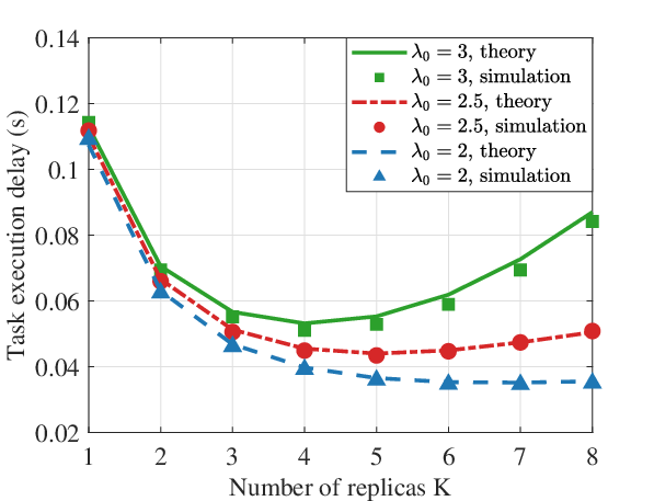
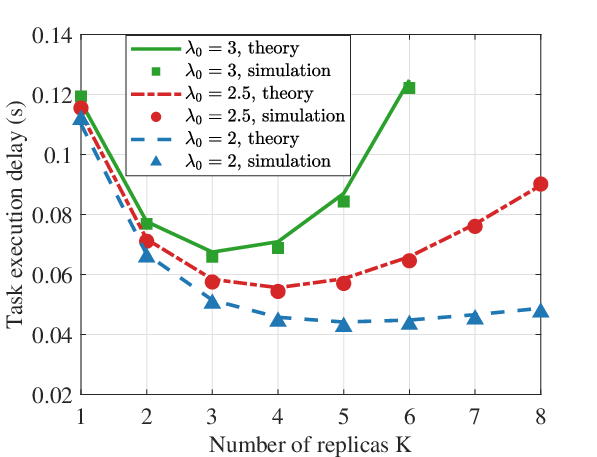
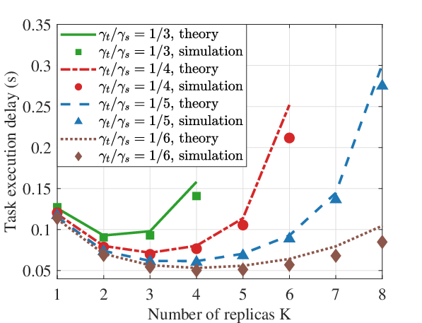
Fig. 2 and Fig. 3 show the average task execution delay with respect to the number of task replicas $K$ under different task arrival rates $\lambda_{0}$ and TaV to SeV density ratios $\frac{\gamma_{t}}{\gamma_{s}}$. Given $\lambda_{0}$ and $\frac{\gamma_{t}}{\gamma_{s}}$, the task execution delay first decreases with $K$ and then increases, and the optimal $K$ varies with the network conditions. A proper number of task replicas can improve the delay performance substantially, compared to the case without replications. For example, as shown in Fig. 2(b), when $\lambda_{0}=4$ and $\frac{\gamma_{t}}{\gamma_{s}}=\frac{1}{3}$, task execution delay with $K=4$ replicas can be decreased by $50\%$ compared to that without replication ($K=1$).

Table I compares the optimal number of task replicas obtained from theory and simulation. Specifically, the task execution delay is calculated according to (10) from $K=1$ to $8$, and $K_{\text{theory}}^{*}$ is the corresponding $K$ that minimizes (10), which is the optimal theoretical result. $K_{\text{sim}}^{*}$ is obtained via Monte Carlo simulation. $\tilde{K}^{*}$ is calculated according to Theorem 1, and $\tilde{K}_{\text{round}}^{*}=\text{round}\left(\tilde{K}^{*}\right)$ is the integer nearest to $\tilde{K}^{*}$, which is our approximated result. Remark that, the main contribution of the analysis is to derive the near-optimal number of task replicas $\tilde{K}^{*}$ that minimizes the average task execution delay, as shown in Theorem 1. Therefore, we mainly validate the accuracy of $\tilde{K}^{*}$ in this part.

We can see from Table I that under most cases, our near-optimal solution $\tilde{K}_{\text{round}}^{*}$ is exactly the same as the optimal theoretical and simulation results. Occasionally, $\tilde{K}_{\text{round}}^{*}$ is not the optimal solution, but it is quite close-to-optimal, with a maximum difference of 1. We remark that, the number of task replicas is always an integer, thus a difference of 1 is a very small gap. Moreover, the task execution delay achieved by $K=\tilde{K}_{\text{round}}^{*}$ and $K=K_{\text{theory}}^{*}$ are very close even if $\tilde{K}_{\text{round}}^{*}\neq K_{\text{theory}}^{*}$. For example, in Table I, when $\lambda_{0}=2$ and $\gamma_{t}/\gamma_{s}=\frac{1}{4}$, $K_{\text{theory}}^{*}=7$ and $\tilde{K}_{\text{round}}^{*}=6$. According to Fig. 2(a), the task execution delay at $K=7$ and $K=6$ are almost the same. In brief, the approximation given in Theorem 1 provides an accurate estimate of the optimal number of task replicas, which can guide the efficient task replication from the system point of view.

To evaluate the offloading delay and reliability of the proposed task replication algorithm, we simulate a realistic traffic scenario in SUMO¹¹ 1 http://www.sumo.dlr.de/userdoc/SUMO.html using a $12\mathrm{km}$ segment of G6 Highway in Beijing, which is downloaded from Open Street Map (OSM)²² 2 http://www.openstreetmap.org/. The traffic scenario is the same as that in Section VI of [24]. The total arrival rate of vehicles in SUMO is set to $0.5$. According to the traffic flow information, the average number of vehicles per $\mathrm{km}$ is roughly $25$, which is close to the settings in the previous subsection. The maximum speed allowed of each TaV or SeV is $20\mathrm{m/s}$. The output of SUMO is the car data, including the location, speed, angle of each vehicle at each time, which is imported to MATLAB for further simulations.

For each task, the input data size is $L_{i}=1\mathrm{Mbits}$, and the output data size is considered to be negligible. For task upload, the path loss exponent is set to $2$, the channel bandwidth $W_{u}=10\mathrm{MHz}$, transmission power $P=0.5\mathrm{W}$, and noise power $N_{0}=10^{-13}\mathrm{W}$. The service rate $\mu_{c}(n)$ of each candidate SeV is uniformly distributed within $[8,12]$ tasks per second, and the packet erasure probability $p_{e}(t,n)$ is uniformly selected within $[0.01,0.03]$, so that the mean service rate $\mu_{c}=10$ and the mean packet erasure probability $p_{e}=0.02$ are the same as above. Moreover, parameter $\alpha$ in (18) is set to $0.5$, the maximum delay $d_{\text{max}}=0.5\mathrm{s}$ and the discretization level $l=100$.

The proposed algorithm is compared to: 1) Genie-aided policy, where the TaV knows the exact global state information of all candidate SeVs, and offloads a single task to the SeV that can provide the minimum delay. Note that genie-aided policy cannot be realized in reality, which is used as a lower bound. 2) Random policy, where the TaV randomly selects a single SeV for each task. 3) Single offloading policy, which is also an MAB-based learning algorithm proposed in [24], where each TaV selects a single SeV to offload each task, and learns the delay performance while offloading.

Fig. 4 shows the evolution of the average offloading delay with respect to the number of offloaded tasks, under different density ratios of TaV to SeV with task arrival rate $\lambda_{0}=4$. In Fig. 4(a), $\frac{\gamma_{t}}{\gamma_{s}}=0$ indicates that the target TaV can monopolize the SeVs instead of sharing with other TaVs. In this case, replication can fully exploit the diversity gain, and the more task replicas are offloaded, the lower task offloading delay can be achieved. When $K=5$, the average offloading delay is very close to that achieved by the genie-aided policy. As $\frac{\gamma_{t}}{\gamma_{s}}$ grows higher, i.e., more TaVs share the wireless channels and SeV computation resources, fewer number of task replicas may achieve better delay performance. For example, in Fig. 4(d), $K=5$ leads to serious overload, so that the delay performance is even worse than that of the random benchmark, while $K=2$ is the optimal choice. Furthermore, the optimal number of task replicas obtained under the realistic traffic scenario coincides with the analytical results. For example, in Fig. 4(c), $K=3$ is the optimal choice, which is the same as $\tilde{K}_{\text{round}}^{*}$ according to Table I when $\frac{\gamma_{t}}{\gamma_{s}}=\frac{1}{4}$ and $\lambda_{0}=4$.

Fig. 5 further plots the average offloading delay and task completion ratio under different task arrival rates and TaV to SeV density ratios. The deadline of each task is set to $d_{\text{max}}=0.5\mathrm{s}$. Overall, task replication significantly improves the delay performance and task completion ratio compared with single task offloading. According to Fig. 5(a) and Fig. 5(c), with a proper replication, the average offloading delay can be reduced by over $56\%$ when the task arrival rate is low ($\lambda_{0}=2$), and by $33\%$ when the task arrival rate is high ($\lambda_{0}=4.5$). Meanwhile, the task completion ratio can be improved from $97\%$ to over $99.6\%$ with proper number of task replicas, as shown in Fig. 5(b) and Fig. 5(d).

References

- [1] Y. Sun, J. Song, S. Zhou, X. Guo, and Z. Niu, “Task replication for vehicular edge computing: A combinatorial multi-armed bandit based approach,” in Proc. IEEE Global Commun. Conf. (GLOBECOM), Abu Dhabi, UAE, Dec. 2018.
- [2] IEEE 802.11 Working Group, “IEEE standard for information technology - Telecommunications and information exchange between systems - Local and metropolitan area networks - Specific requirements - Part 11: Wireless LAN Medium Access Control (MAC) and Physical Layer (PHY) specifications Amendment 6: Wireless Access in Vehicular Environments,” IEEE Std. 802.11, Jul. 2010.
- [3] 3GPP TS 36.300 V14.11.0, “Evolved universal terrestrial radio access (E-UTRA) and evolved universal terrestrial radio access network (E-UTRAN),” Sept. 2019.
- [4] S. Chen, J. Hu, Y. Shi, and L. Zhao, “LTE-V: A TD-LTE-based V2X solution for future vehicular network,” IEEE Internet Things J., vol. 3, no. 6, pp. 997-1005, Dec. 2016.
- [5] Intel, “Self-driving car technology and computing requirements,” [Online] Available: https://www.intel.com/content/www/ us/en/automotive/driving-safety-advanced-driver-assistance-systems-self-driving-technol ogy-paper.html
- [6] Y. Mao, C. You, J. Zhang, K. Huang, and K. B. Letaief, “A survey on mobile edge computing: The communication perspective,” IEEE Commun. Surveys Tuts., vol. 19, no. 4, pp. 2322-2358, 2017.
- [7] P. Mach, and Z. Becvar, “Mobile edge computing: A survey on architecture and computation offloading,” IEEE Commun. Surveys Tut., vol. 19, no. 3, pp. 1628-1656, 2017.
- [8] W. Yu, F. Liang, X. He, W. G. Hatcher, C. Lu, J. Lin, and X. Yang, “A survey on the edge computing for the Internet of things,” IEEE Access, vol. 6, pp. 6900-6919, 2018.
- [9] S. Abdelhamid, H. Hassanein, and G. Takahara, “Vehicle as a resource (VaaR),” IEEE Netw., vol. 29, no. 1, pp. 12-17, Feb. 2015.
- [10] S. Bitam, A. Mellouk, and S. Zeadally, “VANET-cloud: A generic cloud computing model for vehicular ad hoc networks,” IEEE Wireless Commun., vol. 22, no. 1, pp. 96-102, Feb. 2015.
- [11] X. Hou, Y. Li, M. Chen, D. Wu, D. Jin, and S. Chen, “Vehicular fog computing: A viewpoint of vehicles as the infrastructures,” IEEE Trans. Veh. Technol., vol. 65, pp. 3860-3873, Jun. 2016.
- [12] X. Cheng, C. Chen, W. Zhang, and Y. Yang, “5G-enabled cooperative intelligent vehicular (5GenCIV) framework: When Benz meets Marconi,” IEEE Intelligent Systems, vol. 32, no. 3, pp. 53-59, May/June 2017.
- [13] J. S. Choo, M. Kim, S. Pack, and G. Dan, “The software-defined vehicular cloud: A new level of sharing the road,” IEEE Veh. Technol. Mag., vol. 12, no. 2, pp. 78-88, Jun. 2017.
- [14] G. Qiao, S. Leng, K. Zhang and Y. He, “Collaborative task offloading in vehicular edge multi-access networks,” IEEE Commun. Mag., vol. 56, no. 8, pp. 48-54, Aug. 2018.
- [15] S. Zhou, Y. Sun, Z. Jiang, and Z. Niu, “Exploiting moving intelligence: Delay-optimized computation offloading in vehicular fog networks,” IEEE Commun. Mag., vol. 57, no. 5, pp. 49-55, May 2019.
- [16] S. Andreev, V. Petrov, K. Huang, M. A. Lema and M. Dohler, “Dense moving fog for intelligent IoT: Key challenges and opportunities,” IEEE Commun. Mag., vol. 57, no. 5, pp. 34-41, May 2019.
- [17] 3GPP, “Study on enhancement of 3GPP support for 5G V2X services,” 3GPP TR 22.886, V15.1.0, Mar. 2017.
- [18] J. Ni, A. Zhang, X. Lin and X. S. Shen, “Security, Privacy, and Fairness in Fog-Based Vehicular Crowdsensing,” IEEE Commun. Mag., vol. 55, no. 6, pp. 146-152, Jun. 2017.
- [19] K. Zheng, H. Meng, P. Chatzimisios, L. Lei, and X. Shen, “An SMDP-based resource allocation in vehicular cloud computing systems,” IEEE Trans. Ind. Electron., vol. 62, no. 12, pp. 7920-7928, Dec. 2015.
- [20] Z. Jiang, S. Zhou, X. Guo, and Z. Niu, “Task replication for deadline-constrained vehicular cloud computing: Optimal policy, performance analysis and implications on road traffic,” IEEE Internet Things J., vol. 5, no. 1, pp. 93-107, Feb. 2018.
- [21] J. Feng, Z. Liu, C. Wu, and Y. Ji, “AVE: autonomous vehicular edge computing framework with aco-based scheduling,” IEEE Trans. Veh. Technol., vol. 66, no. 12, pp. 10660-10675, Dec. 2017.
- [22] Z. Zhou, H. Liao, X. Zhao, B. Ai, and M. Guizani, “Reliable task offloading for vehicular fog computing under information asymmetry and information uncertainty,” IEEE Trans. Veh. Technol., vol. 68, no. 9, pp. 8322-8335, Sept. 2019.
- [23] Y. Sun, X. Guo, S. Zhou, Z. Jiang, X. Liu, and Z. Niu, “Learning-based task offloading for vehicular cloud computing systems,” IEEE Int. Conf. Commun. (ICC), Kansas city, MO, USA, May 2018.
- [24] Y. Sun, X. Guo, J. Song, S. Zhou, Z. Jiang, X. Liu, and Z. Niu, “Adaptive learning-based task offloading for vehicular edge computing systems,” IEEE Trans. Veh. Technol., vol. 68, no. 4, pp. 3061-3074, Apr. 2019.
- [25] K. Gardner, S. Zbarsky, S. Doroudi, M. Harchol-Balter, and E. Hyytia, “Reducing latency via redundant requests: Exact analysis,” ACM SIGMETRICS Perform. Eval. Rev., vol. 43, no. 1, pp. 347-360, Jun. 2015.
- [26] K. Gardner, M. Harchol-Balter, A. Scheller-Wolf, M. Velednitsky, and S. Zbarsky, “Redundancy-d: The power of d choices for redundancy,” Operations Research, vol. 65, no. 4, pp. 1078-1094, Apr. 2017.
- [27] G. Joshi, E. Soljanin, and G. Wornell. “Efficient redundancy techniques for latency reduction in cloud systems.” ACM Trans. Modeling Perform. Eval. Comput. Syst. (TOMPECS) vol. 2, no. 2, pp. 1-30, Apr. 2017.
- [28] L. Chen, and J. Xu, “Task replication for vehicular cloud: Contextual combinatorial bandit with delayed feedback,” in Proc. IEEE Conference on Computer Communications (INFOCOM), Paris, France, Apr. 2019.
- [29] K. Gardner, M. Harchol-Balter, A. Scheller-Wolf, and B. Van Houdt, “A better model for job redundancy: Decoupling server slowdown and job size,” IEEE/ACM Transactions on Networking, vol. 25, no. 2, pp. 3353-3367, Sept. 2017.
- [30] M. Grundmann, V. Kwatra, M. Han, and I. Essa, “Efficient hierarchical graph-based video segmentation,” in Proc. IEEE Conf. Comput. Vis. Pattern Recog. (CVPR), San Francisco, CA, USA, Jun. 2010.
- [31] K. Sriram, and W. Whitt, “Characterizing superposition arrival processes in packet multiplexers for voice and data,” IEEE J. Sel. Areas Commun., vol. 4, pp. 833-846, Sep. 1986.
- [32] S. Ko, K. Han, and K. Huang, “Wireless Networks for Mobile Edge Computing: Spatial Modeling and Latency Analysis,” IEEE Trans. Wireless Commun., vol. 17, no. 8, pp. 5225-5240, Aug. 2018.
- [33] N. U. Prabhu, “Foundations of queueing theory,” Springer Science & Business Media, Dec. 2012.
- [34] Y. Sun, S. Zhou, and J. Xu, “EMM: Energy-Aware Mobility Management for Mobile Edge Computing in Ultra Dense Networks,” IEEE J. Sel. Areas Commun., vol. 35, no. 11, pp. 2637-2646, Nov. 2017.
- [35] C. You, K. Huang, H. Chae, and B. H. Kim, “Energy-efficient resource allocation for mobile-edge computation offloading,” IEEE Trans. Wireless Commun., vol. 16, no. 3, pp. 1397–1411, Mar. 2016.
- [36] Y. Yao, L. Rao, and X. Liu, “Performance and reliability analysis of IEEE 802.11p safety communication in a highway environment,” IEEE Trans. Veh. Technol., vol. 62, no. 9, pp. 4198-4212, Nov. 2013.
- [37] Y. Yao, L. Rao, X. Liu, and X. Zhou, “Delay analysis and study of IEEE 802.11p based DSRC safety communication in a highway environment,” in Proc. IEEE Int. Conf. on Computer Commun. (INFOCOM), Turin, Italy, Apr. 2013.
- [38] P. Auer, N. Cesa-Bianchi, and P. Fischer, “Finite-time analysis of the multiarmed bandit problem,” Machine learning, vol. 47, no. 2-3, pp. 235–256, May 2002.
- [39] W. Chen, Y. Wang, and Y. Yuan. “Combinatorial multi-armed bandit: General framework and applications,” Int. Conf. on Machine Learning (ICML), Atlanta, GA, USA, Jun. 2013.
- [40] W. Chen, W. Hu, F. Li, J. Li, Y. Liu, and P. Lu, “Combinatorial multi-armed bandit with general reward functions,” Advances in Neural Information Processing Systems, vol. 29, Dec. 2016.
- [41] A. Goel, S. Guha, and K. Munagala, “How to probe for an extreme value,” ACM Trans. on Algorithms, vol. 7, no. 1, Nov. 2010.
- [42] M. Haenggi, “Stochastic geometry for wireless networks,” Cambridge University Press, Oct. 2012.
- [43] K. Lee, M. Lam, R. Pedarsani, D. Papailiopoulos, and K. Ramchandran, “Speeding up distributed machine learning using codes,” IEEE Trans. Inf. Theory, vol. 64, no. 3, pp. 1514-1529, Mar. 2018.
- [44] N. Ferdinand, and S. C. Draper, “Hierarchical coded computation,” in Proc. IEEE Int. Symp. on Inform. Theory (ISIT), Vail, CO, USA, Jun. 2018, pp. 1620-1624.
- [45] Y. Sun, J. Zhao, S. Zhou, and D. Gündüz, “Heterogeneous coded computation across heterogeneous workers,” in Proc. IEEE Global Commun. Conf. (GLOBECOM), Waikoloa, HI, USA, Dec. 2019.