Input Perturbation: A New Paradigm between Central and Local Differential Privacy
Abstract.
Traditionally, there are two models on differential privacy: the central model and the local model. The central model focuses on the machine learning model and the local model focuses on the training data. In this paper, we study the input perturbation method in differentially private empirical risk minimization (DP-ERM), preserving privacy of the central model. By adding noise to the original training data and training with the ‘perturbed data’, we achieve (,)-differential privacy on the final model, along with some kind of privacy on the original data. We observe that there is an interesting connection between the local model and the central model: the perturbation on the original data causes the perturbation on the gradient, and finally the model parameters. This observation means that our method builds a bridge between local and central model, protecting the data, the gradient and the model simultaneously, which is more superior than previous central methods. Detailed theoretical analysis and experiments show that our method achieves almost the same (or even better) performance as some of the best previous central methods with more protections on privacy, which is an attractive result. Moreover, we extend our method to a more general case: the loss function satisfies the Polyak-Lojasiewicz condition, which is more general than strong convexity, the constraint on the loss function in most previous work.
Keywords:
differential privacy, machine learning, input perturbation, empirical risk minimization1. Introduction
In recent years, machine learning has been shown effective in fields such as pattern recognition and data mining (Yee et al. 2018), (Rahman et al. 2018), (Bulgarevich et al. 2018), (Fu et al. 2019) and large quantities of personal data has been collected to support machine learning algorithms. The collection of tremendous data leads a huge problem: the disclosure of personal sensitive information. In real scenarios, not only the leakage of original data will disclose the information of individuals, when training machine learning models, model parameters may reveal sensitive information in an undirect way as well (Shokri et al. 2017), (Fredrikson et al. 2014).
To solve the problem of information leakage, differential privacy (DP) (Dwork 2011), (Dwork et al. 2006) was proposed and has become a popular way to preserve privacy in machine learning. It preserves sensitive information by adding random noise, making an adversary can not infer any single data instance in the dataset by observing model parameters. Differential privacy has received a great deal of attentions and has been applied to regression (Chaudhuri and Monteleoni 2009), (Smith et al. 2018), (Bernstein and Sheldon 2019), boosting (Dwork et al. 2010), (Zhao et al. 2018), PCA (Chaudhuri et al. 2013), (Wang and Xu 2019), GAN (Wu et al. 2019), (Xu et al. 2019), transfer learning (LeTien et al. 2019), graph algorithms (Sealfon and Ullman 2019), (Ullman and Sealfon 2019), (Arora and Upadhyay 2019), deep learning (Shokri and Shmatikov 2015), (Abadi et al. 2016) and other fields.
Empirical risk minimization (ERM), covering a wide variety of machine learning tasks, is also bothered by privacy problems. There is a long list of works on DP-ERM (Wang et al. 2017), (Bassily et al. 2014), (Chaudhuri et al. 2011), (Zhang et al. 2017), (Kifer et al. 2012). According to different ways of adding noise, three approaches were proposed to achieve differential privacy: output perturbation, objective perturbation and gradient perturbation, adding noise to the final model, the objective function and the gradient, respectively.
However, the original data is not preserved by perturbation methods mentioned above. In real scenarios, before training, original data is sent to a ‘data center’, which is trusted in central models, shown in Figure 1 (a). When it comes to the situation that ‘data center’ is not trusted, local differential privacy (LDP) (Beimel et al. 2008), (Kairouz et al. 2014) was proposed to provide plausible deniability, by randomizing the data before releasing it. As shown in Figure 1 (b), LDP focuses on the privacy of the communications between individuals and the ‘server’, rather than the final machine learning model (Duchi et al. 2013), (Wang et al. 2018), (Wang et al. 2019a), (Duchi et al. 2018), (Wang et al. 2019b). However, the noise added for preserving privacy in LDP is always large, compromising predictive performance.

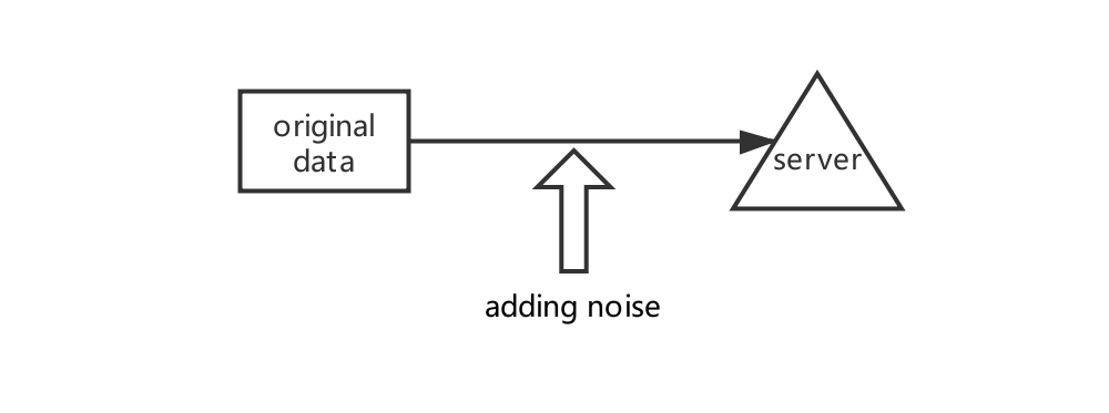

To alleviate the problems mentioned above, in this paper, we study the input perturbation method, achieving (,)-differential privacy on the final model. The comparison between our method and previous perturbation methods is shown in Figure 1. It can be observed that our method focuses on the final model and preserves the original data to some extents. Even if the adversaries get the perturbed data in the ‘data center’, the leakage of sensitive information decreases a lot compared with traditional central models. Actually, adding noise to original data to preserve privacy is commonly used in the field of computer vision (Hill et al. 2016), (Fan 2018), (Lee et al. 2019). In this way, it is not easy to reconstruct the original data (Agrawal and Srikant 2000).
By adding noise to original data, protections are applied before ‘data input’, and our method is more reliable than traditional central models. Moreover, we observe that our input perturbation method also perturbs the gradient and the final model parameters, building a bridge between local and central differential privacy.
Contributions of Our Method
A Bridge between Local and Central Differenital Privacy 0.
By observing a fact that the noise added to data causes perturbation on the gradient and finally the final model, we build a bridge between local and central differential privacy, guaranteeing (,)-differential privacy on the final model along with some kind of privacy on the original data simultaneously. When comparing with traditional central perturbation methods, in which the privacy of original data is ignored, we provide more privacy. Meanwhile, comparing with LDP, we make a balance on the performance and the privacy of individuals: adding less noise and keeping better performance. Additionally, the privacy on the final model remains.
Superior Theoretical and Experimental Results 0.
Detailed theoretical analysis and experiments show that the performance of our method is similar to (or even better than) some of the best previous methods in central setting. Considering that our method preserves both the original data and the final model and other central methods ignore the security of original training data, the results are attractive. When it comes to LDP, although in our method, the privacy between individuals and the ‘data center’ is weaker, the performance of our method is much better, which is a trade-off and the sacrifice is acceptable.
| Method | Noise Type | Noise Bound | Excess Empirical Risk Bound | ||
|---|---|---|---|---|---|
| (Chaudhuri et al. 2011) | Output Perturbation | Yes | |||
| (Chaudhuri et al. 2011) | Objective Perturbation | Yes | |||
| (Kifer et al. 2012) | Objective Perturbation | No | Gaussian Noise2 | ||
| (Bassily et al. 2014) | Gradient Perturbation | No | Gaussian Noise | ||
| (Zhang et al. 2017) | Output Perturbation | No | Gaussian Noise | ||
| (Wang et al. 2017) (DP-SVRG) | Gradient Perturbation | No | Gaussian Noise | ||
| (Wang et al. 2017) (traditional) | Gradient Perturbation | No | Gaussian Noise | ||
| (Duchi et al. 2013) | LDP | Yes | Randomized response | None3 | |
| (Wang et al. 2018) | LDP | Yes | Laplace Noise2 | ||
| (Fukuchi et al. 2017) | Input Perturbation | No | Gaussian Noise | ||
| Our Method | Input Perturbation | No | Gaussian Noise |
- 2
The noise bound of the Gaussian and Laplace noise and are represented by the variance, whose means are 0.
- 3
The noise added by randomized response is complicated, details can be found in (Duchi et al. 2013).
- 4
is the size of training set, is the number of total iterations, is the number of model parameters, input has -dimensional feature.
A More General Condition 0.
Considering that most previous works assume the loss function is strongly convex, we generalize it to the condition that the loss function satisfies the Polyak-Lojasiewicz condition, which is more general than strong convexity.
The rest of the paper is organized as follows. In Section 2, we introduce some works related to our method. We introduce some basic definitions and formulations in Section 3. In Section 4, we propose our method: input perturbation in detail. In Section 5, we give the theoretical analysis of our method and extend it to a more general case. We present the experimental results in Section 6. Finally, we conclude the paper in Section 7.
2. RELATED WORK
In this section, we introduce some work on private ERM methods and list the comparison of their theoretical results.
The first work on DP-ERM was proposed in (Chaudhuri et al. 2011), in which two methods were proposed: output perturbation and objective perturbation. The probability density function of the noise , where is a normalizing constant, is a function of the privacy budget and denotes -norm. In this work, the derivative of the loss function was assumed -Lipschitz. Based on these assumptions, it provided theoretical analysis on the noise bound and the excess empirical risk bound. The noise of the method proposed in (Chaudhuri et al. 2011) was improved by (Kifer et al. 2012). The improved noise is related to the upper bound of , (i.e. for all ). Additionally, this work assumed the perturbed objective function is -strongly convex, and gives the excess empirical risk bound, which is related to the noise and the optimal model .
By gradient perturbation, (Bassily et al. 2014) added noise to the gradient, guaranteeing differential privacy by assuming that the loss function is -Lipschitz. Like in (Chaudhuri et al. 2011), (Zhang et al. 2017) proposed an output perturbation method, achieving a better excess empirical bound. Advanced gradient descent method Prox-SVRG (Xiao and Zhang 2014) was introduced in (Wang et al. 2017), and a new algorithm DP-SVRG was proposed. DP-SVRG achieved optimal or near optimal utility bounds with less gradient complexity. In this work, the noise bound was related to , the sampling iterations in the algorithm DP-SVRG. Note that in DP-SVRG, better results are because of advanced gradient descent method, rather than advanced perturbation method.
However, all the methods proposed in previous work are based on output perturbation, objective perturbation or gradient perturbation. As a result, privacy preserving is after ‘data input’, which increases the risk of information leakage. Although LDP can solve the problem of ‘untrusted data center’, the theoretical results are much worse, which can be observed in Table 111 1 The theoretical results of LDP and input perturbation in Table 1 are simplified, more details can be found in (Wang et al. 2018), (Duchi et al. 2013) and (Fukuchi et al. 2017)..
Under these circumstances, input perturbation was proposed in (Fukuchi et al. 2017), in which although noise is added to data, it achieves differential privacy by constructing a ‘perturbed objective function’. It guarantees (,)-LDP and (,)-central DP. However, considering that is always large, the LDP is unsatisfactory. Moreover, its excess empirical risk bound is also much weaker than some central models because the noise added to the original data is large.
Considering the problems mentioned above, in this paper, we focus on input perturbation, adding noise to the original data and training machine learning model by the ‘perturbed data’. By observing the effects caused by input perturbation: noise added to the data leads perturbation on the gradient and the final model parameters, our method provides (,)-differential privacy on the final model, which is the same as central setting, along with some kinds of protections on original data, showing the connections between local and central differential privacy. Theoretical comparisons between our method and previous methods are shown in Table 1.
It can be observed that the noise bound of our method is better than the gradient perturbation method proposed in (Wang et al. 2017). For which the advanced gradient descent algorithm DP-SVRG is used, the difference is by a factor of . For traditional gradient descent method in (Wang et al. 2017), the difference is . When comparing with the method proposed in (Bassily et al. 2014), our method is much better, the difference is up to . When it comes to the input perturbation method proposed in (Fukuchi et al. 2017), our noise bound is better than it approximately by a factor of .
The excess empirical risk bound of our method is related to the upper bound of the -norm of the model parameters, (i.e. ). Our method is better than traditional gradient perturbation method proposed in (Bassily et al. 2014) by a factor of , almost , considering can be seemed as a constant. When comparing with the methods proposed in (Wang et al. 2017), our method achieves almost the same excess empirical risk bound, the difference is approximately , no matter the advanced gradient descent algorithm, DP-SVRG, is used or not. In some scenarios that (such as neural network), this gap can be ignored. Meanwhile, the excess empirical risk bound of our method is much better than the input perturbation method proposed in (Fukuchi et al. 2017), approximately by a factor of , which is a huge gap. Considering that the (,)-LDP guaranteed by the input perturbation method proposed in (Fukuchi et al. 2017) is unsatisfactory (actually, this privacy is really weak because is always up to hundreds or thousands), the sacrifice on LDP for the improvement on performance in our method is acceptable.
In this paper, we add noise to data, leading the perturbation on the gradient and achieves (,)-differential privacy on the model parameter, building a bridge between local and central differential privacy. By detailed analysis, it can be observed that the theoretical results of our method are similar to (or even better than) previous central perturbation methods. Experimental results also show that the performance of our proposed method is similar to the gradient perturbation method proposed in (Wang et al. 2017) and the output perturbation method proposed in (Zhang et al. 2017). Our method preserves the privacy of the gradient, (,)-differential privacy on final model parameters along with some kind of original data privacy, without decreases on theoretical or practical results, which is an attractive result.
3. PRELIMINARIES
In this section, first, we introduce some basic definitions, including the comparison between central and local differential privacy. Then, we list traditional perturbation methods of central differentially private ERM in detail: output perturbation, objective perturbation and gradient perturbation.
3.1. Notations and Basic Definitions
Given a -dimensional vector =, denotes its -norm by =. Two databases differing by one element are denoted by , called adjacent databases.
Definition 1 (Central Differential Privacy (Dwork et al. 2014)).
A randomized function is (,)-differential privacy if
| (1) |
where range() and is the number of parameters.
Definition 2 (Local Differential Privacy (Wang et al. 2019a)).
An algorithm is (,)-local differential privacy if for all , and for all events in the output space of , we have:
| (2) |
According to the definitions of central and local differential privacy, in Definition 1, datasets and are input to the randomized function , the privacy of the machine learning model is focused, guaranteeing information cannot be inferred by observing the machine learning model. In Definition 2, records and are input to the algorithm , data is paid more attention, guaranteeing information cannot be inferred by observing the ‘noisy data’. In the local model, ‘untrusted server’ is seemed as the malicious adversary.
3.2. Traditional Perturbation Methods
Our method focuses more on the privacy of the machine learning model, similar to the central setting. So, in this part, we introduce three traditional central perturbation methods.
In general, the objective function of ERM without privacy preserving is defined as:
| (3) |
where denotes data instance, is the loss function.
In the case of binary classification, the data space and the label set , and we assume throughout that is the unit ball so that .
Output Perturbation 0.
In output perturbation, noise is directly added to the model (in the paper, we denote model by parameters):
| (4) |
where is the noise guaranteeing differential privacy.
Output Perturbation method is commonly used because it is simple to implement, only adding noise to the final model.
Objective Perturbation 0.
In the method of objective perturbation, noise is added to the objective function:
| (5) |
The perturbed objective function is directly optimized:
| (6) |
Note that in (5), there may be some other terms on the right side of the equality, for example in (Kifer et al. 2012). We only list the most important term to guarantee differential privacy here.
This method is rarely used in recent years because it is always a trouble to optimize the perturbed objective function and the performance is unsatisfactory.
Gradient Perturbation 0.
In the gradient perturbation method, noise is added to the gradient when training, which leads the gradient descent process at round to:
| (7) |
where is the learning rate.
After iterations in total, the final model .
Because most machine learning algorithms are based on gradient descent method, gradient perturbation is feasible and popular.
4. DIFFERENTIALLY PRIVATE ERM WITH INPUT PERTURBATION
In this section, first, we analyze the weaknesses of traditional central perturbation methods and local models introduced in Section 3, then we propose our method input perturbation in detail.
When training models, original data is always sent to the ‘data center’ in advance, which is shown in Figure 1. By observing three traditional perturbation methods of central DP-ERM, original data is not protected, which means the ‘data center’ is assumed trusted.
However, ‘data center’ is not easy to ‘trust’ because the adversaries always desire to ‘take away’ the original data and the ‘data center’ may be monitored with high probability. As a result, the security of original data instances is of the same importance as (or even more important than) the model parameters. LDP is a superior way to solve the problem of ‘untrusted data center’, guaranteeing differential privacy over the communications (data exchanging) between individuals and the ‘data center’. However, as shown in Table 1, the noise added to data is large, and it is inevitable that the performance is worse than central models.
To solve the problems mentioned above, we propose a new input perturbation method, adding noise to data instances and training the machine learning model by the ‘perturbed data instances’, which leads the objective function to:
| (8) |
In order to distinguish with the objective function without privacy consideration in (3), we denote the objective function of input perturbation by . In (8), ‘noise adding’ has been done in advance and the formulation is for distinguishing the perturbed data and original data.
Our method focuses on achieving (,)-differential privacy on the machine learning model with some kind of privacy on original data. As a result, even if the ‘data center’ is not trusted or monitored, the data ‘taken away’ by malicious adversaries is with random noise, which preserves the ‘true original data’ of individuals from some kinds of attacks.
Although in our method, noise is added to the original data, we focus more on the (,)-differential privacy of the final model, which is different from the local model: protections between individuals and the ‘server’ are paid more attentions, and the privacy of model parameters is not discussed. Comparing with LDP and input perturbation method in (Fukuchi et al. 2017), based on the aim to guarantee the quality of the machine learning model, we sacrifice some of the privacy on individuals for the performance. In fact, the sacrifice compared with (Fukuchi et al. 2017) is not much. In other words, focusing on keeping good performance, we attempt to preserve the privacy on original data as much as possible. It can be observed that in LDP and previous input perturbation method, the noise added to data is much more than ours. As a result, the privacy preserving on individuals of our method is weaker than in LDP and previous input perturbation method, but still stronger than central methods.
Our method is detailed in Algorithm 1.
In Algorithm 1, the random noise and each element , sampled independently. By line 7 in Algorithm 1, it can be seen that the noise added to the original data affects the gradient. The theoretical analysis of our method in Section 5 is based on this observation.
Besides, by observing that our method adds noise to original data instances, leading perturbation on the gradient and eventually causing perturbation on the model parameters, a bridge is built between local and central differential privacy: input perturbation ERM protects the original data, the gradient and the final model simultaneously, giving a higher level privacy compared with traditional central perturbation methods without decreases on the theoretical or practical results. Meanwhile, we achieve better performance compared with LDP and previous input perturbation method, by sacrificing some amount of privacy on individuals.
5. THEORETICAL ANALYSIS OF INPUT PERTURBATION ERM
In this section, first, we give privacy guarantees of our proposed method: input perturbation ERM. Then, we analyze the excess empirical risk bound of our method. Finally, we extend our method to a more general case, in which the loss function is not restricted strongly convex but satisfies the Polyak-Lojasiewicz condition, which is more general than the property ‘strongly convex’.


5.1. Differential Privacy
In this part, we analyze the (,)-differential privacy of our proposed method: input perturbation in Algorithm 1.
In this paper, we analyze -differential privacy by Gaussian mechanism proposed in (Dwork et al. 2006) and moments accountant proposed in (Abadi et al. 2016). Moreover, we assume is like in (Chaudhuri et al. 2011).
Theorem 1.
In Algorithm 1, for , if is -Lipschitz and -strongly convex over and
| (9) |
it is (,)-differential privacy for some constant .
The proof is detailed in the Appendix.
It can be observed that by using our method, the noise added to data instances is almost the same as the gradient perturbation method proposed in (Wang et al. 2017). The difference is by a factor of , which can be seen as a constant. When comparing with the traditional gradient perturbation method proposed in (Bassily et al. 2014), our noise bound is much better than it by a factor up to . Meanwhile, the noise bound of our method is far better than LDP methods, considering that LDP preserves stronger privacy between individuals and the ‘server’, and our method pays more attentions on the privacy of the final machine learning model, this result is conceivable.
The similarity between our method and the gradient perturbation method is the same as our observation: perturbation on original data causes the perturbation on gradients, which builds a bridge between local and central differential privacy. As a result, our proposed input perturbation method achieves (,)-DP on the final model through this ‘bridge’. Hence, our method preserves the privacy of the original data instances, the gradient and the model parameters simultaneously, providing a higher level protection on privacy in a more reliable way in the field of central DP-ERM.
5.2. Excess Empirical Risk Bound
In this part, we analyze the utility of our proposed method and give the excess empirical risk bound, denoted by the expectation of , where is the value of the objective function over the optimal model without privacy consideration. Formally, , where is the same as in (3).
Theorem 2.
Suppose that is -Lipschitz, is -Lipschitz55 5 -Lipschitz on means -smooth on . and the -norm of the model parameter has an upper bound (i.e. for all ), with is the same as in (9), we have:
| (10) |
where , represents the learning rate and each data instance has -dimensional features.
The proof is shown in the Appendix.
Remark 1.
Considering that the smoothness of the objective function after input perturbation is not easy to achieve because of the existence of the random variable , we assume (without random variables) is -smooth, which is easier to hold, making the utility and the excess empirical risk bound of our method feasible.
It can be observed that the excess empirical risk bound of our method is better than the traditional gradient perturbation method proposed in (Bassily et al. 2014) by a factor of . Considering that the variables can be seemed as constants, our method in much better than which proposed in (Bassily et al. 2014) by a factor of . When comparing with gradient perturbation methods proposed in (Wang et al. 2017), the gap on empirical risk bound is by a factor of . In some cases that , which is common in the field such as deep learning, the gap between our method and the gradient perturbation methods proposed in (Wang et al. 2017) is relatively small and can be ignored. When it comes to the comparison between our method and LDP methods, the excess empirical risk bound of our method is much better, with weaker privacy on individuals.
5.3. More general condition
In this part, we extend our method to a more general condition that the loss function is not restricted -strongly convex, but satisfies the Polyak-Lojasiewicz condition.
Definition 3.
Given a function , if there exists and for all , we have:
| (11) |
then satisfies the Polyak-Lojasiewicz condition.
The Polyak-Lojasiewicz condition is much more general than strongly convex. It was shown in (Karimi et al. 2016) that when function is differential and -smooth under -norm, we have:
Strong Convex Essential Strong Convexity Weak Strongly Convexity Restricted Secant Inequality Polyak-Lojasiewicz Inequality Error Bound
Theorem 3.
In Algorithm 1, for , if the loss function is -Lipschitz and satisfies Polyak-Lojasiewicz condition over and
| (12) |
it is (,)-differential privacy for some constant .
Detailed proof is shown in the Appendix.
Theorem 4.
Suppose that is -Lipschitz, is -Lipschitz, is -smooth over and the -norm of the model parameter has an upper bound (i.e. ), with is the same as in (52), we have:
| (13) |
where , is the learning rate and each data instance has -dimensional features.
The proof of Theorem 4 is almost the same as Theorem 2, with replacement of .
By Theorem 3 and Theorem 4, it can be observed that in a more general case: the loss function is not restricted strongly convex but satisfies the Polyak-Lojasiewicz condition, our noise bound and the excess empirical risk bound are almost the same as previous work on central models.
6. EXPERIMENTS
The experiments are performed on the classification task. Considering that our method focuses on the privacy of the final model, the experiments are applied on central methods: the objective perturbation method proposed in (Kifer et al. 2012), the output perturbation method proposed in (Zhang et al. 2017) and the gradient perturbation methods proposed in (Bassily et al. 2014) and (Wang et al. 2017) (without DP-SVRG). The performance is represented by accuracy and the optimality gap, the latter is defined as . Accuracy represents the performance on test data and optimal gap denotes excess empirical risk on training data.
According to the sizes of datasets, we use logistic regression model (LR) and deep learning model on the datasets KDDCup99 (Hettich and Bay 1999), Adult (Dua and Graff 2017), Bank (Moro et al. 2014), where the total number of data instances are 70000, 45222 and 41188, the sizes are large than 10000. On datasets Breast Cancer (Mangasarian and Wolberg 1990), Credit Card Fraud (Bontempi and Worldline 2018), Iris (Dua and Graff 2017), only logistic regression model is applied because the sizes are less than 1000, where the total number of data instances are 699, 984 and 150, respectively. In the experiments, deep learning model is denoted by Multi-layer Perceptron (MLP) with one hidden layer whose size is the same as the input layer. The training set and the testing set are chosen randomly.
In all experiments, and are chosen by cross-validation. We evaluate the influence over differential privacy budget , which is set from 0.01 to 0.25. Meanwhile, is set according to the size of datasets and can be seemed as a constant. Note that in logistic regression model, and in deep learning model, .
Figure 2 shows that the accuracy of our proposed method is better than the gradient perturbation method proposed in (Bassily et al. 2014) and the objective perturbation method proposed in (Kifer et al. 2012). And our method is almost the same as the gradient perturbation method proposed in (Wang et al. 2017) and the output perturbation method proposed in (Zhang et al. 2017) on accuracy, no matter on the LR model or on the MLP model. However, because the variance of the Gaussian noise added to the gradient in the method (Bassily et al. 2014) is large: , the accuracy of this method over fluctuates sharply in Figure 2.
It can be observed that in Figure 3, the optimality gap of our method is almost the same as the output perturbation method proposed in (Wang et al. 2017) and is better than other methods mentioned above over most datasets, which is similar to the theoretical analysis. Moreover, it can be observed that the optimality gap of our method on some datasets are close to 0, which means that our method achieves almost the same performance as the ERM model without privacy consideration in some scenarios, on both LR model and MLP model. In addition, like the accuracy in Figure 2, the optimality gap of the gradient perturbation method proposed in (Bassily et al. 2014) fluctuates sharply because of its noise bound.
Figure 4 shows accuracy and optimality gap on small datasets (the sizes are less than 1000), in which only logistic regression model is applied. The results are similar to which in Figure 2 and Figure 3, which means that our method is effective in most cases.
By observing the experimental results, we find that although there are slight differences in experimental results on different datasets, the performance of the gradient perturbation method proposed in (Bassily et al. 2014) and the objective perturbation method proposed in (Kifer et al. 2012) is much weaker than our method, the former is because of its loose noise bound and the latter is because of the perturbation method itself. Our proposed method: input perturbation, is almost the same as (on some datasets, even better than) the output perturbation method in (Wang et al. 2017) and the traditional gradient perturbation method without DP-SVRG in (Zhang et al. 2017) on both accuracy and optimality gap, which is similar to our theoretical analysis in Section 4. The experimental results on the deep learning model (MLP), are similar to the traditional machine learning (logistic regression) model. Considering that our method preserves the privacy of the original data, the gradient and the final model simultaneously, providing more privacy without decreases on the performance compared with previous central methods, it is an attractive result.
7. CONCLUSIONS
In this paper, we study the input perturbation method in DP-ERM, adding Gaussian noise to original data instances and training the machine learning model by the ‘perturbed data’. By observing that input perturbation leads the perturbation on the gradient and finally the perturbation on the final model, we build a bridge between local and central differential privacy, achieving (,)-differential privacy on the final machine learning model, along with some kind of privacy on individuals. Through the ‘bridge’, we preserve the original data, the gradient and the final machine learning model simultaneously. Meanwhile, we extend our method to a more general condition, in which the loss function is not considered strongly convex but satisfies the Polyak-Lojasiewicz condition. Theoretical analysis and experiments (applied on both traditional machine learning model: logistic regression, and deep learning model: MLP) on real datasets show that our method achieves almost the same (or even better) performance compared with some of the best previous methods. Additionally, higher level of privacy is achieved, comparing with previous central methods. It is worth emphasizing that our method adds noise to original data, independent of specific optimization methods, which means that our proposed method is a general paradigm. Moreover, detailed analysis of the privacy preserved on individuals of our method and how to improve the privacy of individuals will also be paid attentions in future work.
References
- (1)
- Abadi et al. (2016) Martin Abadi, Andy Chu, Ian Goodfellow, H Brendan McMahan, Ilya Mironov, Kunal Talwar, and Li Zhang. 2016. Deep learning with differential privacy. In Proceedings of the 2016 ACM SIGSAC Conference on Computer and Communications Security. 308–318.
- Agrawal and Srikant (2000) Rakesh Agrawal and Ramakrishnan Srikant. 2000. Privacy-preserving data mining. In ACM Sigmod Record, Vol. 29. 439–450.
- Arora and Upadhyay (2019) Raman Arora and Jalaj Upadhyay. 2019. On Differentially Private Graph Sparsification and Applications. In Advances in Neural Information Processing Systems 32, H. Wallach, H. Larochelle, A. Beygelzimer, F. d'Alché-Buc, E. Fox, and R. Garnett (Eds.). Curran Associates, Inc., 13378–13389. http://papers.nips.cc/paper/9494-on-differentially-private-graph-sparsification-and-applications.pdf
- Bassily et al. (2014) Raef Bassily, Adam Smith, and Abhradeep Thakurta. 2014. Private empirical risk minimization: Efficient algorithms and tight error bounds. In 2014 IEEE 55th Annual Symposium on Foundations of Computer Science. 464–473.
- Beimel et al. (2008) Amos Beimel, Kobbi Nissim, and Eran Omri. 2008. Distributed private data analysis: Simultaneously solving how and what. In Annual International Cryptology Conference. Springer, 451–468.
- Bernstein and Sheldon (2019) Garrett Bernstein and Daniel R Sheldon. 2019. Differentially Private Bayesian Linear Regression. In Advances in Neural Information Processing Systems 32, H. Wallach, H. Larochelle, A. Beygelzimer, F. d'Alché-Buc, E. Fox, and R. Garnett (Eds.). Curran Associates, Inc., 523–533. http://papers.nips.cc/paper/8343-differentially-private-bayesian-linear-regression.pdf
- Bontempi and Worldline (2018) Gianluca Bontempi and Worldline. 2018. ULB The Machine Learning Group. http://mlg.ulb.ac.be
- Bulgarevich et al. (2018) Dmitry S Bulgarevich, Susumu Tsukamoto, Tadashi Kasuya, Masahiko Demura, and Makoto Watanabe. 2018. Pattern recognition with machine learning on optical microscopy images of typical metallurgical microstructures. Scientific reports 8, 1 (2018), 2078.
- Bun and Steinke (2016) Mark Bun and Thomas Steinke. 2016. Concentrated differential privacy: Simplifications, extensions, and lower bounds. In Theory of Cryptography Conference. Springer, 635–658.
- Chaudhuri and Monteleoni (2009) Kamalika Chaudhuri and Claire Monteleoni. 2009. Privacy-preserving logistic regression. In Advances in neural information processing systems. 289–296.
- Chaudhuri et al. (2011) Kamalika Chaudhuri, Claire Monteleoni, and Anand D Sarwate. 2011. Differentially private empirical risk minimization. Journal of Machine Learning Research 12, Mar (2011), 1069–1109.
- Chaudhuri et al. (2013) Kamalika Chaudhuri, Anand D Sarwate, and Kaushik Sinha. 2013. A near-optimal algorithm for differentially-private principal components. The Journal of Machine Learning Research 14, 1 (2013), 2905–2943.
- Csiba and Richtárik (2017) Dominik Csiba and Peter Richtárik. 2017. Global Convergence of Arbitrary-Block Gradient Methods for Generalized Polyak-L ojasiewicz Functions. arXiv preprint arXiv:1709.03014 (2017).
- Dua and Graff (2017) Dheeru Dua and Casey Graff. 2017. UCI Machine Learning Repository. http://archive.ics.uci.edu/ml
- Duchi et al. (2013) John C Duchi, Michael I Jordan, and Martin J Wainwright. 2013. Local privacy and statistical minimax rates. In 2013 IEEE 54th Annual Symposium on Foundations of Computer Science. 429–438.
- Duchi et al. (2018) John C Duchi, Michael I Jordan, and Martin J Wainwright. 2018. Minimax optimal procedures for locally private estimation. J. Amer. Statist. Assoc. 113, 521 (2018), 182–201.
- Dwork (2011) Cynthia Dwork. 2011. Differential privacy. Encyclopedia of Cryptography and Security (2011), 338–340.
- Dwork et al. (2006) Cynthia Dwork, Frank McSherry, Kobbi Nissim, and Adam Smith. 2006. Calibrating noise to sensitivity in private data analysis. In Theory of cryptography conference. Springer, 265–284.
- Dwork et al. (2014) Cynthia Dwork, Aaron Roth, et al. 2014. The algorithmic foundations of differential privacy. Foundations and Trends® in Theoretical Computer Science 9, 3–4 (2014), 211–407.
- Dwork et al. (2010) Cynthia Dwork, Guy N Rothblum, and Salil Vadhan. 2010. Boosting and differential privacy. In 2010 IEEE 51st Annual Symposium on Foundations of Computer Science. 51–60.
- Fan (2018) Liyue Fan. 2018. Image pixelization with differential privacy. In IFIP Annual Conference on Data and Applications Security and Privacy. Springer, 148–162.
- Fredrikson et al. (2014) Matthew Fredrikson, Eric Lantz, Somesh Jha, Simon Lin, David Page, and Thomas Ristenpart. 2014. Privacy in pharmacogenetics: An end-to-end case study of personalized warfarin dosing. In 23rd USENIX Security Symposium (USENIX Security 14). 17–32.
- Fu et al. (2019) Geng-Shen Fu, Yuri Levin-Schwartz, Qiu-Hua Lin, and Da Zhang. 2019. Machine Learning for Medical Imaging. Journal of healthcare engineering 2019 (2019).
- Fukuchi et al. (2017) Kazuto Fukuchi, Quang Khai Tran, and Jun Sakuma. 2017. Differentially Private Empirical Risk Minimization with Input Perturbation. In International Conference on Discovery Science. Springer, 82–90.
- Hettich and Bay (1999) S. Hettich and S. D. Bay. 1999. The UCI KDD Archive [http://kdd.ics.uci.edu].
- Hill et al. (2016) Steven Hill, Zhimin Zhou, Lawrence Saul, and Hovav Shacham. 2016. On the (in) effectiveness of mosaicing and blurring as tools for document redaction. Proceedings on Privacy Enhancing Technologies 2016, 4 (2016), 403–417.
- Kairouz et al. (2014) Peter Kairouz, Sewoong Oh, and Pramod Viswanath. 2014. Extremal mechanisms for local differential privacy. In Advances in neural information processing systems. 2879–2887.
- Karimi et al. (2016) Hamed Karimi, Julie Nutini, and Mark Schmidt. 2016. Linear convergence of gradient and proximal-gradient methods under the polyak-łojasiewicz condition. In Joint European Conference on Machine Learning and Knowledge Discovery in Databases. Springer, 795–811.
- Kifer et al. (2012) Daniel Kifer, Adam Smith, and Abhradeep Thakurta. 2012. Private convex empirical risk minimization and high-dimensional regression. In Conference on Learning Theory. 25–1.
- Lee et al. (2019) Kangwook Lee, Hoon Kim, Kyungmin Lee, Changho Suh, and Kannan Ramchandran. 2019. Synthesizing Differentially Private Datasets using Random Mixing. In 2019 IEEE International Symposium on Information Theory (ISIT). 542–546.
- LeTien et al. (2019) Nam LeTien, Amaury Habrard, and Marc Sebban. 2019. Differentially Private Optimal Transport: Application to Domain Adaptation. In Proceedings of the Twenty-Eighth International Joint Conference on Artificial Intelligence, IJCAI-19. International Joint Conferences on Artificial Intelligence Organization, 2852–2858. https://doi.org/10.24963/ijcai.2019/395
- Mangasarian and Wolberg (1990) Olvi L Mangasarian and William H Wolberg. 1990. Cancer diagnosis via linear programming. Technical Report. University of Wisconsin-Madison Department of Computer Sciences.
- Moro et al. (2014) Sérgio Moro, Paulo Cortez, and Paulo Rita. 2014. A data-driven approach to predict the success of bank telemarketing. Decision Support Systems 62 (2014), 22–31.
- Rahman et al. (2018) Quazi Abidur Rahman, Tahir Janmohamed, Meysam Pirbaglou, Hance Clarke, Paul Ritvo, Jane M Heffernan, and Joel Katz. 2018. Defining and Predicting Pain Volatility in Users of the Manage My Pain App: Analysis Using Data Mining and Machine Learning Methods. Journal of medical Internet research 20, 11 (2018), e12001.
- Sealfon and Ullman (2019) Adam Sealfon and Jonathan Ullman. 2019. Efficiently Estimating Erdos-Renyi Graphs with Node Differential Privacy. arXiv preprint arXiv:1905.10477 (2019).
- Shokri and Shmatikov (2015) Reza Shokri and Vitaly Shmatikov. 2015. Privacy-preserving deep learning. In Proceedings of the 22nd ACM SIGSAC conference on computer and communications security. 1310–1321.
- Shokri et al. (2017) Reza Shokri, Marco Stronati, Congzheng Song, and Vitaly Shmatikov. 2017. Membership inference attacks against machine learning models. In 2017 IEEE Symposium on Security and Privacy (SP). 3–18.
- Smith et al. (2018) M Smith, Alvarez Lopez, M Zwiessele, and N Lawrence. 2018. Differentially Private Regression using Gaussian Processes. In Proceedings of Machine Learning Research, Vol. 84.
- Ullman and Sealfon (2019) Jonathan Ullman and Adam Sealfon. 2019. Efficiently Estimating Erdos-Renyi Graphs with Node Differential Privacy. In Advances in Neural Information Processing Systems 32, H. Wallach, H. Larochelle, A. Beygelzimer, F. d'Alché-Buc, E. Fox, and R. Garnett (Eds.). Curran Associates, Inc., 3765–3775. http://papers.nips.cc/paper/8633-efficiently-estimating-erdos-renyi-graphs-with-node-differential-privacy.pdf
- Wang et al. (2018) Di Wang, Marco Gaboardi, and Jinhui Xu. 2018. Empirical risk minimization in non-interactive local differential privacy revisited. In Advances in Neural Information Processing Systems. 965–974.
- Wang et al. (2019a) Di Wang, Adam Smith, and Jinhui Xu. 2019a. Noninteractive locally private learning of linear models via polynomial approximations. In Algorithmic Learning Theory. 897–902.
- Wang and Xu (2019) Di Wang and Jinhui Xu. 2019. Principal Component Analysis in the Local Differential Privacy Model. In Proceedings of the Twenty-Eighth International Joint Conference on Artificial Intelligence, IJCAI-19. International Joint Conferences on Artificial Intelligence Organization, 4795–4801. https://doi.org/10.24963/ijcai.2019/666
- Wang et al. (2017) Di Wang, Minwei Ye, and Jinhui Xu. 2017. Differentially private empirical risk minimization revisited: Faster and more general. In Advances in Neural Information Processing Systems. 2722–2731.
- Wang et al. (2019b) Ning Wang, Xiaokui Xiao, Yin Yang, Jun Zhao, Siu Cheung Hui, Hyejin Shin, Junbum Shin, and Ge Yu. 2019b. Collecting and Analyzing Multidimensional Data with Local Differential Privacy. In 2019 IEEE 35th International Conference on Data Engineering (ICDE). 638–649.
- Wu et al. (2019) Bingzhe Wu, Shiwan Zhao, Haoyang Xu, ChaoChao Chen, Li Wang, Xiaolu Zhang, Guangyu Sun, and Jun Zhou. 2019. Generalization in Generative Adversarial Networks: A Novel Perspective from Privacy Protection. arXiv preprint arXiv:1908.07882 (2019).
- Xiao and Zhang (2014) Lin Xiao and Tong Zhang. 2014. A proximal stochastic gradient method with progressive variance reduction. SIAM Journal on Optimization 24, 4 (2014), 2057–2075.
- Xu et al. (2019) Chugui Xu, Ju Ren, Deyu Zhang, Yaoxue Zhang, Zhan Qin, and Kui Ren. 2019. GANobfuscator: Mitigating information leakage under GAN via differential privacy. IEEE Transactions on Information Forensics and Security 14, 9 (2019), 2358–2371.
- Yee et al. (2018) Ong Shu Yee, Saravanan Sagadevan, and Nurul Hashimah Ahamed Hassain Malim. 2018. Credit card fraud detection using machine learning as data mining technique. Journal of Telecommunication, Electronic and Computer Engineering (JTEC) 10, 1-4 (2018), 23–27.
- Zhang et al. (2017) Jiaqi Zhang, Kai Zheng, Wenlong Mou, and Liwei Wang. 2017. Efficient private ERM for smooth objectives. arXiv preprint arXiv:1703.09947 (2017).
- Zhao et al. (2018) Lingchen Zhao, Lihao Ni, Shengshan Hu, Yaniiao Chen, Pan Zhou, Fu Xiao, and Libing Wu. 2018. InPrivate Digging: Enabling Tree-based Distributed Data Mining with Differential Privacy. In IEEE INFOCOM 2018-IEEE Conference on Computer Communications. 2087–2095.
Appendix A Details of Proof
A.1. Theorem 1
Proof.
By observing that the noise added to data causes the perturbation on the gradient, we pay our attentions on the gradient descent descent process:
| (14) |
where and denotes the learning rate.
Then, considering about the query which may disclose privacy, the randomized mechanism is:
| (15) |
Denote probability distributions on adjacent databases and over mechanism as and :
| (16) | ||||
where we suppose that the single different data instance between and is the one, denoted as and , respectively.
For simplicity on expression, we set:
| (17) | ||||
In moments accountant method proposed in (Abadi et al. 2016), the moment on mechanism is defined as:
| (19) |
where is privacy loss at the output , defined as:
| (20) |
When it comes to privacy preserving, it is necessary to bound all possible , denoted as , which is defined as:
| (21) |
By Definition 2.1 in (Bun and Steinke 2016), is defined as:
| (22) |
By (23) and Lemma 2.5 in (Bun and Steinke 2016), we have:
| (24) |
By definitions of and in (17) and note that is -Lipschitz (), we have:
| (25) |
By (Csiba and Richtárik 2017), if function is -strongly convex (), we have:
| (26) |
In general, with the increasing of training iteration, loss of the model decreases. i.e. if . So, we have:
| (28) |
Considering that can be seemed as a constant, by (25) and (28), for some constant , (24) can be transferred to:
| (29) |
By Theorem 2.1 in (Abadi et al. 2016), we have:
| (30) |
By summing over iterations on (29), for some constant :
| (31) |
Taking for some constant , we can guarantee:
| (32) |
and as a result, we have:
| (33) |
leading -differential privacy according to Theorem 2.2 in (Abadi et al. 2016). ∎
A.2. Theorem 2
Proof.
First, considering at round :
| (34) |
Note that is -Lipschitz (), then for all :
| (35) |
By the definition of in (8), we have:
| (37) |
Note that is -Lipschitz (), then we have:
| (38) |
Note that and , (39) can be transferred to:
| (40) |
For random variable X, we have:
| (42) |
where denotes the variance of X.
By summing (43) over iterations and note that :
| (44) |
Then, considering the gap between and :
| (45) | ||||
If is -smooth, we have:
| (46) |
where denotes the optimal model and .
Taking the same as in (9), we have:
| (49) |
when , where the notation is similar to , but hiding factors polynomial in and . ∎
A.3. Theorem 3
Proof.
Taking the same as in A.1.
Note that the loss function satisfies the Polyak-Lojasiewicz condition (), we have:
| (50) |
As a result, in the moments accountant method:
| (51) |
The factor can be seemed as a constant, then:
| (52) |
for some constant .
By summing iterations, for some constant , we have:
| (53) |
Taking the same as in (9), it can be guaranteed that:
| (54) |
and as a result:
| (55) |
for some constant , which means ()-differential privacy due to Theorem 2.2 in (Abadi et al. 2016). ∎