跳到论文正文
W Papers独立论文阅读器 arXiv:2002.08561 论文正文 计算阅读时间 · 0%
引用这篇论文根据当前论文元数据生成,正式投稿前建议核对。


License: arXiv.org perpetual non-exclusive license
arXiv:2002.08561v2 [math.OC] 17 Mar 2020

Column Partition based Distributed Algorithms for Coupled Convex Sparse Optimization: Dual and Exact Regularization Approaches

Jinglai Shen Note: J. Shen and Eswar Kumar H.K. are with Department of Mathematics and Statistics, University of Maryland Baltimore County, Baltimore, MD 21250, U.S.A. Emails: shenj@umbc.edu and eswar1@umbc.edu.    Jianghai Hu Note: J. Hu is with the School of Electrical and Computer Engineering, Purdue University, West Lafayette, IN 47907, U.S.A. E-mail: jianghai@purdue.edu.       Eswar Kumar Hathibelagal Kammara
Abstract

This paper develops column partition based distributed schemes for a class of large-scale convex sparse optimization problems, e.g., basis pursuit (BP), LASSO, basis pursuit denosing (BPDN), and their extensions, e.g., fused LASSO. We are particularly interested in the cases where the number of (scalar) decision variables is much larger than the number of (scalar) measurements, and each agent has limited memory or computing capacity such that it only knows a small number of columns of a measurement matrix. These problems in consideration are densely coupled and cannot be formulated as separable convex programs using column partition. To overcome this difficulty, we consider their dual problems which are separable or locally coupled. Once a dual solution is attained, it is shown that a primal solution can be found from the dual of corresponding regularized BP-like problems under suitable exact regularization conditions. A wide range of existing distributed schemes can be exploited to solve the obtained dual problems. This yields two-stage column partition based distributed schemes for LASSO-like and BPDN-like problems; the overall convergence of these schemes is established using sensitivity analysis techniques. Numerical results illustrate the effectiveness of the proposed schemes.

1 Motivation and Introduction

Sparse modeling and approximation finds broad applications in numerous fields of contemporary interest, including signal and image processing, compressed sensing, machine learning, and high dimensional statistics and data analytics. Various efficient schemes have been proposed for convex or nonconvex sparse signal recovery [9, 21]. To motivate the work of this paper, consider the well-studied LASSO problem: minx∈ℝN⁡12​‖A​x−b‖22+λ​‖x‖1,\min_{x\in\mathbb{R}^{N}}\ \frac{1}{2}\|Ax-b\|^{2}_{2}+\lambda\,\|x\|_{1}, where A∈ℝm×NA\in\mathbb{R}^{m\times N} is the measurement (or sensing) matrix, b∈ℝmb\in\mathbb{R}^{m} is the measurement (or sensing) vector, λ>0\lambda>0 is the penalty parameter, and x∈ℝNx\in\mathbb{R}^{N} is the decision variable. In the setting of sparse recovery, NN is much larger than mm. Besides, the measurement matrix AA usually satisfies certain uniform recovery conditions for recovery efficiency, e.g., the restricted isometry property [9]. As such, AA is often a dense matrix, namely, (almost) all of its elements are nonzero. We aim to develop distributed algorithms to solve the LASSO and other relevant problems, where each agent only knows the vector bb and a small subset of the columns of AA. Specifically, let {ℐ1,…,ℐp}\{\mathcal{I}_{1},\ldots,\mathcal{I}_{p}\} be a disjoint union of {1,…,N}\{1,\ldots,N\} such that {A∙ℐi}i=1p\{A_{\bullet\mathcal{I}_{i}}\}^{p}_{i=1} forms a column partition of AA. For each ii, the iith agent only has the knowledge of bb and A∙ℐiA_{\bullet\mathcal{I}_{i}}. By running the proposed distributed scheme, it is expected that each agent ii attains the subvector of an optimal solution of the LASSO corresponding to the index set ℐi\mathcal{I}_{i}, i.e., xℐi∗x^{*}_{\mathcal{I}_{i}}, at the end of the scheme, where x∗x^{*} denotes an optimal solution of the LASSO.

The distributed optimization task described above is inspired by the following two scenarios arising from big data and network systems, respectively. In the context of big data, a practitioner may deal with a ultra-large data set, e.g., NN is extremely large, so that it would be impossible to store a vector x∈ℝNx\in\mathbb{R}^{N} in a single computing device, let alone the measurement matrix AA. When mm is relatively small compared with NN, the proposed distributed schemes can be used where each device only needs to store the vector bb and a small number of the columns of AA. The second scenario arises from multi-agent network systems, where each agent is operated by a low cost computing device which has limited memory and computing capacities. Hence, even when NN is moderately large, it would be impractical for the entire matrix AA to be stored or computed on one of these devices. Therefore, the proposed distributed schemes can be exploited in this scenario. Besides, the proposed algorithms can be extended to other sub-matrix partitions (in both row and column) of AA, even if mm is large in the above scenarios.

Centralized algorithms for the LASSO and other related convex sparse optimization problems, e.g., BP and BPDN, have been extensively studied, and can be categorized into the first-order methods [2, 9, 13, 26, 28], and the second-order methods [4, 14]. A number of effective distributed or decentralized schemes have also been developed, for example, [11, 15, 16, 18, 23, 29], just to name a few. To the best of our knowledge, most of the current distributed or decentralized schemes for the LASSO and BPDN require the central knowledge of the entire AA in at least one step of these schemes (which are referred to as partially distributed); exceptions include [16, 29] for distributed basis pursuit using the dual approach. In contrast, the distributed schemes developed in this paper do not require the knowledge of the entire AA for any agent throughout the schemes and are fully distributed. A major difficulty of developing column partition based fully distributed schemes for the LASSO and BPDN problems is that they are densely coupled. Recently, distributed schemes are developed for locally coupled convex programs [11]. However, since AA is a dense matrix, the loss function ‖A​x−b‖22\|Ax-b\|^{2}_{2} cannot be written in a locally coupled manner over a general network. Hence, the technique in [11] cannot be directly applied to the LASSO and BPDN.

The development of the proposed distributed algorithms relies on several key techniques in convex optimization, including dual problems, solution properties of the LASSO and BPDN, exact regularization, distributed computing of separable convex programs, and sensitivity analysis. First, motivated by the dual approach for distributed BP [16, 29], we consider the Lagrangian dual problems of LASSO and BPDN, which are separable or locally coupled and thus can be solved via column partition based distributed schemes. By using the solution properties of the LASSO and BPDN, we show that a primal solution is a solution of a basis pursuit-like (BP-like) problem depending on a dual solution. Under exact regularization conditions, a primal solution can be obtained from the dual of a regularized BP-like problem which can be solved by another column partition based distributed scheme. This leads to two-stage, column partition based distributed schemes for the LASSO and BPDN, where many existing distributed schemes or methods (e.g., distributed consensus optimization and distributed averaging schemes) can be used at each stage. The overall convergence of the two-stage schemes is established via sensitivity analysis of the BP-like problem. The proposed schemes are applicable to a broad class of generalized BP, LASSO and BPDN under mild assumptions on communication networks; we only assume that a network is static, connected and bidirectional. Extensions to time-varying networks can be made.

The rest of the paper is organized as follows. In Section 2, we formulate the BP, LASSO, BPDN and their extensions, and discuss basic solution properties. Exact regularization of these problems is investigated in Section 3. Section 4 establishes their dual problems and studies properties in connection with the primal problems. Based on these results, column partition based fully distributed schemes are developed in Section 5, including two-stage distributed schemes for the LASSO-like and BPDN-like problems whose overall convergence is shown in Section 6 via sensitivity analysis tools. Finally, numerical results are given in Section 7, and conclusions are drawn in Section 8.

Notation. Let AA be an m×Nm\times N real matrix. For any index set 𝒮⊆{1,…,N}\mathcal{S}\subseteq\{1,\ldots,N\}, let A∙𝒮A_{\bullet\mathcal{S}} be the matrix formed by the columns of AA indexed by elements of 𝒮\mathcal{S}. Similarly, for an index set α⊆{1,…,m}\alpha\subseteq\{1,\ldots,m\}, Aα∙A_{\alpha\bullet} is the matrix formed by the rows of AA indexed by elements of α\alpha. Let {ℐi}i=1p\{\mathcal{I}_{i}\}^{p}_{i=1} form a disjoint union of {1,…,N}\{1,\ldots,N\}, and {xℐi}i=1p\{x_{\mathcal{I}_{i}}\}^{p}_{i=1} form a partition of x∈ℝNx\in\mathbb{R}^{N}. For a∈ℝna\in\mathbb{R}^{n}, let a+:=max⁡(a,0)≥0a_{+}:=\max(a,0)\geq 0 and a−:=max⁡(−a,0)≥0a_{-}:=\max(-a,0)\geq 0. For a closed convex set 𝒞\mathcal{C} in ℝn\mathbb{R}^{n}, Π𝒞\Pi_{\mathcal{C}} denotes the Euclidean projection operator onto 𝒞\mathcal{C}. For u,v∈ℝnu,v\in\mathbb{R}^{n}, u⟂vu\perp v stands for the orthogonality of uu and vv, i.e., uT​v=0u^{T}v=0.

2 Problem Formulation and Solution Properties

We consider a class of convex sparse minimization problems and their generalizations or extensions whose formulations are given as follows.

∙\bullet Basis Pursuit (BP) and Extensions. This problem intends to recover a sparse vector from noiseless measurement bb given by the following linear equality constrained optimization problem

BP:minx∈ℝN∥x∥1subject toAx=b,\text{BP}:\quad\underset{x\in\mathbb{R}^{N}}{\text{min}}\ \|x\|_{1}\quad\text{subject to}\quad Ax=b, (1)

where we assume b∈R⁡(A)b\in R(A). Geometrically, this problem seeks to minimize the 11-norm distance from the origin to the affine set defined by A​x=bAx=b. A generalization of the BP (1) is minx∈ℝN⁡‖E​x‖1\min_{x\in\mathbb{R}^{N}}\|Ex\|_{1} subject to A​x=bAx=b, where E∈ℝr×NE\in\mathbb{R}^{r\times N} is a matrix.

∙\bullet Least Absolute Shrinkage and Selection Operator (LASSO) and Extensions. The standard LASSO intends to minimize the loss function ‖A​x−b‖22\|Ax-b\|^{2}_{2} along with the ℓ1\ell_{1}-norm penalty on xx treated as a convex relaxation of the sparsity of xx:

LASSO:minx∈ℝN12∥Ax−b∥22+λ∥x∥1,\text{LASSO}:\quad\underset{x\in\mathbb{R}^{N}}{\text{min}}\ \frac{1}{2}\|Ax-b\|^{2}_{2}+\lambda\,\|x\|_{1}, (2)

where λ>0\lambda>0 is the penalty parameter. A generalized LASSO is given by minx∈ℝN​12​‖A​x−b‖22+‖E​x‖1,\underset{x\in\mathbb{R}^{N}}{\text{min}}\ \frac{1}{2}\|Ax-b\|^{2}_{2}+\|Ex\|_{1}, where E∈ℝr×NE\in\mathbb{R}^{r\times N} is a given matrix. It includes several extensions and variations of the standard LASSO:

  • (i)

    Fused LASSO: minx∈ℝN⁡12​‖A​x−b‖22+λ1​‖x‖1+λ2​‖D1​x‖1\min_{x\in\mathbb{R}^{N}}\ \frac{1}{2}\|Ax-b\|^{2}_{2}+\lambda_{1}\,\|x\|_{1}+\lambda_{2}\|D_{1}x\|_{1}, where D1∈ℝ(N−1)×ND_{1}\in\mathbb{R}^{(N-1)\times N} denotes the first order difference matrix. Letting E:=[λ1​INλ2​D1]E:=\begin{bmatrix}\lambda_{1}I_{N}\\ \lambda_{2}D_{1}\end{bmatrix}, the fused LASSO can be converted to the generalized LASSO.

  • (ii)

    Generalized total variation denoising and ℓ1\ell_{1}-trend filtering [12]. A generalized total variation denoising is a generalized LASSO with E=λ​D1E=\lambda D_{1} for λ>0\lambda>0, whereas the generalized ℓ1\ell_{1}-trend filtering has E=λ​D2E=\lambda D_{2}, where D2D_{2} is the second order difference matrix.

Another related LASSO problem is the group LASSO, which is widely used in statistics for model selection [30]. For a vector partition {xℐi}i=1p\{x_{\mathcal{I}_{i}}\}^{p}_{i=1} of x∈ℝNx\in\mathbb{R}^{N}, the group LASSO with λi>0\lambda_{i}>0 is given by

minx∈ℝN​12​‖A​x−b‖22+∑i=1pλi​‖xℐi‖2.\underset{x\in\mathbb{R}^{N}}{\text{min}}\ \frac{1}{2}\|Ax-b\|^{2}_{2}+\sum^{p}_{i=1}\lambda_{i}\|x_{\mathcal{I}_{i}}\|_{2}. (3)

∙\bullet Basis Pursuit Denoising (BPDN) and Extensions. Consider the following constrained optimization problem which incorporates noisy signals:

BPDN:minx∈ℝN∥x∥1subject to∥Ax−b∥2≤σ,\text{BPDN}:\quad\underset{x\in\mathbb{R}^{N}}{\text{min}}\ \|x\|_{1}\ \quad\text{subject to}\quad\|Ax-b\|_{2}\leq\sigma, (4)

where σ>0\sigma>0 characterizes the bound of noise or errors. Note that when σ=0\sigma=0, it reduces to the basis pursuit. We assume that ‖b‖2>σ\|b\|_{2}>\sigma since otherwise, x∗=0x_{*}=0 is the trivial solution. Similar to the LASSO, the BPDN has several generalizations and extensions. For example, it can be extended to minx∈ℝN⁡‖E​x‖1\min_{x\in\mathbb{R}^{N}}\|Ex\|_{1} subject to ‖A​x−b‖2≤σ\|Ax-b\|_{2}\leq\sigma, where E∈ℝr×NE\in\mathbb{R}^{r\times N} is a matrix.

We summarize some fundamental solution properties of the aforementioned problems to be used in the subsequent development. For the convenience of generalizations and extensions, we treat the aforementioned problems in a more general setting. Let the constant q>1q>1, E∈ℝr×NE\in\mathbb{R}^{r\times N} be a matrix, ∥⋅∥⋆\|\cdot\|_{\star} be a norm on the Euclidean space, and 𝒞\mathcal{C} be a polyhedral set. Consider the following problems:

(P1):\displaystyle(P_{1}): minx∈ℝN⁡‖E​x‖⋆ subject to A​x=b, and ​x∈𝒞\displaystyle\quad\min_{x\in\mathbb{R}^{N}}\ \|Ex\|_{\star}\quad\mbox{ subject to }\quad Ax=b,\ \mbox{ and }x\in\mathcal{C} (5)
(P2):\displaystyle(P_{2}): minx∈ℝN⁡12​‖A​x−b‖qq+‖E​x‖⋆ subject to x∈𝒞\displaystyle\quad\min_{x\in\mathbb{R}^{N}}\ \frac{1}{2}\|Ax-b\|^{q}_{q}+\|Ex\|_{\star}\quad\mbox{ subject to }\quad x\in\mathcal{C} (6)
(P3):\displaystyle(P_{3}): minx∈ℝN⁡‖E​x‖⋆ subject to ‖A​x−b‖q≤σ​ and x∈𝒞.\displaystyle\qquad\qquad\ \ \min_{x\in\mathbb{R}^{N}}\ \|Ex\|_{\star}\quad\mbox{ subject to }\quad\|Ax-b\|_{q}\leq\sigma\ \mbox{ and }\quad x\in\mathcal{C}. (7)

Note that all the BP, LASSO, and BPDN models introduced before can be formulated within the above framework. For example, in the group LASSO, ‖x‖⋆:=∑i=1pλi​‖xℐi‖2\|x\|_{\star}:=\sum^{p}_{i=1}\lambda_{i}\|x_{\mathcal{I}_{i}}\|_{2} is a norm. Letting E:=INE:=I_{N} and q=2q=2, the group LASSO is a special case of (P2)(P_{2}).

Proposition 2.1.

Fix q>1q>1, and assume that the problems (P1)(P_{1})-(P3)(P_{3}) are feasible. The following hold:

  • (i)

    Each of the problems (P1)−(P3)(P_{1})-(P_{3}) attains a minimizer;

  • (ii)

    Let ℋ2\mathcal{H}_{2} be the solution set of (P2)(P_{2}). Then A​x=A​x′Ax=Ax^{\prime} and ‖E​x‖⋆=‖E​x′‖⋆\|Ex\|_{\star}=\|Ex^{\prime}\|_{\star} for all x,x′∈ℋ2x,x^{\prime}\in\mathcal{H}_{2};

  • (iii)

    Suppose in (P3)(P_{3}) that ‖b‖q>σ\|b\|_{q}>\sigma, 0∈𝒞0\in\mathcal{C}, and the optimal value of (P3)(P_{3}) is positive. Then each minimizer x∗x_{*} of (P3)(P_{3}) satisfies ‖A​x∗−b‖q=σ\|Ax_{*}-b\|_{q}=\sigma and A​xAx is constant on the solution set.

Proof.

Statements (i) and (ii) follow from a similar proof of [17, Theorem 4.1] and [31, Lemma 4.1], respectively. For Statement (iii), by a similar argument of [31, Lemma 4.2(3)], we have that any minimizer x∗x_{*} of (P3)(P_{3}) satisfies ‖A​x∗−b‖q=σ\|Ax_{*}-b\|_{q}=\sigma. Since ∥⋅∥qq\|\cdot\|^{q}_{q} is strictly convex for q>1q>1 [20, Appendix] and ‖A​x−b‖qq\|Ax-b\|^{q}_{q} is constant (whose value is σq\sigma^{q}) on the solution set, we deduce that A​xAx is constant on the solution set. ∎

A sufficient condition for the optimal value of (P3)(P_{3}) to be positive, along with the conditions that ‖b‖q>σ\|b\|_{q}>\sigma and 0∈𝒞0\in\mathcal{C}, is that EE has full column rank. In fact, when ‖b‖q>σ\|b\|_{q}>\sigma and 0∈𝒞0\in\mathcal{C}, any minimizer x∗x_{*} must be nonzero. If EE has full column rank, then E​x∗≠0Ex_{*}\neq 0 so that ‖E​x∗‖⋆>0\|Ex_{*}\|_{\star}>0.

To compute a solution of the LASSO in (11) using its dual solution, we need the following result similar to [31, Theorem 2.1] or [17, Proposition 3.2]. To be self-contained, we present its proof below.

Proposition 2.2.

The following hold:

  • (i)

    Let x∗x_{*} be a minimizer of (P2)(P_{2}) given by (6). Then z∗z_{*} is a minimizer of (P2)(P_{2}) if and only if z∗z_{*} is a minimizer of the BP-like problem given by (5), i.e., (P1):minz∈ℝN⁡‖E​z‖⋆​ subject to ​A​z=A​x∗​ and ​z∈𝒞.(P_{1}):\ \min_{z\in\mathbb{R}^{N}}\ \|Ez\|_{\star}\mbox{ subject to }Az=Ax_{*}\mbox{ and }\ z\in\mathcal{C}. Furthermore, the optimal value of (P1)(P_{1}) equals ‖E​x∗‖⋆\|Ex_{*}\|_{\star}.

  • (ii)

    Let x∗x_{*} be a minimizer of (P3)(P_{3}) given by (7) which satisfies: ‖b‖q>σ\|b\|_{q}>\sigma, 0∈𝒞0\in\mathcal{C}, and the optimal value of (P3)(P_{3}) is positive. Then z∗z_{*} is a minimizer of (P3)(P_{3}) if and only if z∗z_{*} is a minimizer of the BP-like problem (5) with b:=A​x∗b:=Ax_{*}, and the optimal value of this (P1)(P_{1}) equals ‖E​x∗‖⋆\|Ex_{*}\|_{\star}.

Proof.

(i) Let ℋ2\mathcal{H}_{2} be the solution set of (P2)(P_{2}) given by (6). By Proposition 2.1, A​x=A​x∗Ax=Ax_{*} and ‖E​x‖⋆=‖E​x∗‖⋆\|Ex\|_{\star}=\|Ex_{*}\|_{\star} for any x∈ℋ2x\in\mathcal{H}_{2}. Let J⁡(x):=12​‖A​x−y‖qq+‖E​x‖⋆J(x):=\frac{1}{2}\|Ax-y\|^{q}_{q}+\|Ex\|_{\star} be the objective function. For the “if” part, let z∗z_{*} be a minimizer of (P1)(P_{1}). Then z∗∈𝒞z_{*}\in\mathcal{C}, A​z∗=A​x∗Az_{*}=Ax_{*} and ‖E​z∗‖⋆≤‖E​x∗‖⋆\|Ez_{*}\|_{\star}\leq\|Ex_{*}\|_{\star}. Hence, J⁡(z∗)≤J⁡(x∗)J(z_{*})\leq J(x_{*}). On the other hand, J⁡(x∗)≤J⁡(z∗)J(x_{*})\leq J(z_{*}) because x∗x_{*} is a minimizer of (P2)(P_{2}). Therefore, J⁡(x∗)=J⁡(z∗)J(x_{*})=J(z_{*}) so that z∗z_{*} is a minimizer of (P2)(P_{2}). It also implies that ‖E​z∗‖⋆=‖E​x∗‖⋆\|Ez_{*}\|_{\star}=\|Ex_{*}\|_{\star} or equivalently the optimal value of (P1)(P_{1}) equals ‖E​x∗‖⋆\|Ex_{*}\|_{\star}. To show the “only if” part, let z∗z_{*} be a minimizer of (P2)(P_{2}). Suppose z∗z_{*} is not a minimizer of (P1)(P_{1}). Then there exists u∈ℝNu\in\mathbb{R}^{N} such that u∈𝒞u\in\mathcal{C}, A​u=A​x∗Au=Ax_{*} and ‖E​u‖⋆<‖E​z∗‖⋆\|Eu\|_{\star}<\|Ez_{*}\|_{\star}. Since z∗z_{*} is a minimizer of (P2)(P_{2}), we have A​z∗=A​x∗Az_{*}=Ax_{*} and ‖E​z∗‖⋆=‖E​x∗‖⋆\|Ez_{*}\|_{\star}=\|Ex_{*}\|_{\star}. Hence, J⁡(u)<J⁡(z∗)J(u)<J(z_{*}), yielding a contradiction.

(ii) Suppose (P3)(P_{3}) satisfies the specified conditions, and let ℋ3\mathcal{H}_{3} denote its solution set. By statement (iii) Proposition 2.1, we have ℋ3={x∈𝒞|Ax=Ax∗,∥Ex∥⋆=∥Ex∗∥⋆}\mathcal{H}_{3}=\{x\in\mathcal{C}\,|\,Ax=Ax_{*},\,\|Ex\|_{\star}=\|Ex_{*}\|_{\star}\} for a minimizer x∗x_{*} of (P3)(P_{3}). “If”: suppose z∗z_{*} be a minimizer of (P1)(P_{1}) with b:=A​x∗b:=Ax_{*}. Then z∗∈𝒞z_{*}\in\mathcal{C}, A​z∗=A​x∗Az_{*}=Ax_{*} and ‖E​z∗‖⋆≤‖E​x∗‖⋆\|Ez_{*}\|_{\star}\leq\|Ex_{*}\|_{\star}. This shows that z∗z_{*} is a feasible point of (P3)(P_{3}) and hence a minimizer in view of ‖E​z∗‖⋆=‖E​x∗‖⋆\|Ez_{*}\|_{\star}=\|Ex_{*}\|_{\star}. “Only if”: since any feasible point of (P1)(P_{1}) with b:=A​x∗b:=Ax_{*} is a feasible point of (P3)(P_{3}) and since x∗x_{*} is a feasible point of this (P1)(P_{1}), we see that the optimal value of this (P1)(P_{1}) equals ‖E​x∗‖⋆\|Ex_{*}\|_{\star}. Suppose z∗z_{*} is a minimizer of (P3)(P_{3}). Then z∗∈ℋ3z_{*}\in\mathcal{H}_{3} such that z∗∈𝒞z_{*}\in\mathcal{C}, A​z∗=A​x∗Az_{*}=Ax_{*}, and ‖E​z∗‖⋆=‖E​x∗‖⋆\|Ez_{*}\|_{\star}=\|Ex_{*}\|_{\star}. Hence z∗z_{*} is a feasible point of this (P1)(P_{1}) and thus a minimizer of this (P1)(P_{1}). ∎

3 Exact Regularization

A key step in the development of column partition based distributed algorithms is using dual problems. To establish a relation between solutions of a primal problem and its dual, we consider regularization of the primal problem, which is expected to give rise to a solution of the original primal problem. This pertains to the exact regularization of the original primal problem [8].

We briefly review the exact regularization of general convex programs given in [8]. Consider the convex minimization problem (P)(P) and its regularized problem (Pε)(P_{\varepsilon}) for some ε≥0\varepsilon\geq 0:

(P):minx∈𝒫f(x);(Pε):minx∈𝒫f(x)+εh(x),(P):\quad\min_{x\in\mathcal{P}}f(x);\qquad\qquad(P_{\varepsilon}):\quad\min_{x\in\mathcal{P}}f(x)+\varepsilon h(x),

where f,h:ℝN→ℝf,h:\mathbb{R}^{N}\rightarrow\mathbb{R} are real-valued convex functions, and 𝒫\mathcal{P} is a closed convex set. It is assumed that (P)(P) has a solution, and hh is coercive such that (Pε)(P_{\varepsilon}) has a solution for each ε>0\varepsilon>0. A weaker assumption can be made for hh; see [8, Section 1.2] for details. We call the problem (P)(P) exactly regularized if there exists ε¯>0\overline{\varepsilon}>0 such that for any ε∈(0,ε¯]\varepsilon\in(0,\overline{\varepsilon}], any solution of (Pε)(P_{\varepsilon}) is a solution of (P)(P). To establish the exact regularization, consider the following convex program: letting f∗f_{*} be the optimal value of (P)(P),

(Ph):minx∈𝒫,f⁡(x)≤f∗h(x).(P_{h}):\quad\min_{x\in\mathcal{P},\,f(x)\leq f_{*}}\,h(x).

Clearly, the constraint set of (Ph)(P_{h}) is equivalent to {x|x∈𝒫,f(x)=f∗}\{x\,|\,x\in\mathcal{P},f(x)=f_{*}\}, which is the solution set of (P)(P). It is shown in [8, Theorem 2.1] or [8, Corollary 2.2] that (P)(P) is exactly regularized by the regularization function hh if and only if (Ph)(P_{h}) has a Lagrange multiplier μ∗≥0\mu_{*}\geq 0, i.e., there exists a constant μ∗≥0\mu_{*}\geq 0 such that minx∈𝒫,f⁡(x)≤f∗⁡h⁡(x)=minx∈𝒫⁡h⁡(x)+μ∗​(f⁡(x)−f∗).\min_{x\in\mathcal{P},\,f(x)\leq f_{*}}\,h(x)=\min_{x\in\mathcal{P}}\,h(x)+\mu_{*}\big(\,f(x)-f_{*}\big).

Corollary 3.1.

The problem (Ph)(P_{h}) has a Lagrange multiplier μ∗≥0\mu_{*}\geq 0 if and only if there exists a constant μ≥0\mu\geq 0 such that a minimizer x∗x_{*} of (Ph)(P_{h}) is a minimizer of minx∈𝒫⁡h⁡(x)+μ⁡(f⁡(x)−f∗)\min_{x\in\mathcal{P}}h(x)+\mu(f(x)-f_{*}).

Proof.

“If”: suppose a constant μ≥0\mu\geq 0 exists such that a minimizer x∗x_{*} of (Ph)(P_{h}) is that of minx∈𝒫⁡h⁡(x)+μ⁡(f⁡(x)−f∗)\min_{x\in\mathcal{P}}h(x)+\mu(f(x)-f_{*}). Since x∗x_{*} is a feasible point of (Ph)(P_{h}), we have x∗∈𝒫x_{*}\in\mathcal{P} and f⁡(x∗)≤f∗f(x_{*})\leq f_{*} or equivalently f⁡(x∗)=f∗f(x_{*})=f_{*}. Hence, the optimal value of minx∈𝒫⁡h⁡(x)+μ⁡(f⁡(x)−f∗)\min_{x\in\mathcal{P}}h(x)+\mu(f(x)-f_{*}) is given by h⁡(x∗)h(x_{*}), which equals minx∈𝒫,f⁡(x)≤f∗⁡h⁡(x)\min_{x\in\mathcal{P},\,f(x)\leq f_{*}}\,h(x). Hence, μ∗:=μ≥0\mu_{*}:=\mu\geq 0 is a Lagrange multiplier of (Ph)(P_{h}).

“Only If”: Let μ∗≥0\mu_{*}\geq 0 be a Lagrange multiplier of (Ph)(P_{h}), and x∗x_{*} be a minimizer of (Ph)(P_{h}). Again, we have x∗∈𝒫x_{*}\in\mathcal{P} and f⁡(x∗)=f∗f(x_{*})=f_{*}. This shows that h⁡(x∗)+μ∗​(f⁡(x∗)−f∗)=h⁡(x∗)h(x_{*})+\mu_{*}(f(x_{*})-f_{*})=h(x_{*}). Hence,

h⁡(x∗)=minx∈𝒫,f⁡(x)≤f∗⁡h⁡(x)=minx∈𝒫⁡h⁡(x)+μ∗​(f⁡(x)−f∗)≤h⁡(x∗).h(x_{*})\,=\,\min_{x\in\mathcal{P},\,f(x)\leq f_{*}}h(x)\,=\,\min_{x\in\mathcal{P}}\,h(x)+\mu_{*}\big(\,f(x)-f_{*}\big)\leq h(x_{*}).

We thus deduce that x∗x_{*} is a minimizer of minx∈𝒫⁡h⁡(x)+μ⁡(f⁡(x)−f∗)\min_{x\in\mathcal{P}}h(x)+\mu(f(x)-f_{*}) with μ:=μ∗\mu:=\mu_{*}. ∎

3.1 Exact Regularization of Convex Piecewise Affine Function based Optimization

We consider the exact regularization of convex piecewise affine functions based convex minimization problems with its applications to ℓ1\ell_{1}-minimization given by the BP, LASSO, and BPDN. A real-valued continuous function f:ℝN→ℝf:\mathbb{R}^{N}\rightarrow\mathbb{R} is piecewise affine (PA) if there exists a finite family of real-valued affine functions {fi}i=1ℓ\{f_{i}\}^{\ell}_{i=1} such that h⁡(x)∈{fi​(x)}i=1ℓh(x)\in\{f_{i}(x)\}^{\ell}_{i=1} for each x∈ℝNx\in\mathbb{R}^{N}. A convex PA function f:ℝN→ℝf:\mathbb{R}^{N}\rightarrow\mathbb{R} has the max-formulation [19, Section 19], i.e., there exists a finite family of (pi,γi)∈ℝN×ℝ,i=1,…,ℓ(p_{i},\gamma_{i})\in\mathbb{R}^{N}\times\mathbb{R},i=1,\ldots,\ell such that f⁡(x)=maxi=1,…,ℓ⁡(piT​x+γi)f(x)=\max_{i=1,\ldots,\ell}\,\big(\,p^{T}_{i}x+\gamma_{i}\,\big). Convex PA functions represent an important class of nonsmooth convex functions in many applications, e.g., the ℓ1\ell_{1}-norm ∥⋅∥1\|\cdot\|_{1}, f⁡(x):=‖E​x‖1f(x):=\|Ex\|_{1} for a matrix EE, a polyhedral gauge, and the ℓ∞\ell_{\infty}-norm; see [17] for more discussions. We first present a technical lemma whose proof is omitted.

Lemma 3.1.

Let f:ℝN→ℝf:\mathbb{R}^{N}\rightarrow\mathbb{R} and h:ℝN→ℝh:\mathbb{R}^{N}\rightarrow\mathbb{R} be (not necessarily convex) functions and 𝒫\mathcal{P} be a set such that minx∈𝒫⁡f⁡(x)\min_{x\in\mathcal{P}}f(x) attains a minimizer and its optimal value is denoted by f∗f_{*}. Let the set 𝒲:={(x,t)|x∈𝒫,f(x)≤t}\mathcal{W}:=\{(x,t)\,|\,x\in\mathcal{P},f(x)\leq t\}. Consider the following problems:

(Pε):minx∈𝒫f(x)+εh(x);(Pε′):min(x,t)∈𝒲t+εh(x),ε≥0;\displaystyle(P_{\varepsilon}):\quad\min_{x\in\mathcal{P}}f(x)+\varepsilon h(x);\qquad\ (P^{\prime}_{\varepsilon}):\quad\min_{(x,t)\in\mathcal{W}}t+\varepsilon h(x),\qquad\varepsilon\geq 0;
(Ph):minx∈𝒫,f⁡(x)≤f∗h(x);(Ph′):min(x,t)∈𝒲,t≤f∗h(x).\displaystyle(P_{h}):\quad\min_{x\in\mathcal{P},\,f(x)\leq f_{*}}h(x);\ \ \qquad(P^{\prime}_{h}):\quad\min_{(x,t)\in\mathcal{W},\,t\leq f_{*}}h(x).

Then the following hold:

  • (i)

    Fix an arbitrary ε≥0\varepsilon\geq 0. Then (a) if x∗x_{*} is an optimal solution of (Pε)(P_{\varepsilon}), then (x∗,f⁡(x∗))(x_{*},f(x_{*})) is an optimal solution of (Pε′)(P^{\prime}_{\varepsilon}); (b) if (x∗,t∗)(x_{*},t_{*}) is an optimal solution of (Pε′)(P^{\prime}_{\varepsilon}), then t∗=f⁡(x∗)t_{*}=f(x_{*}) and x∗x_{*} is an optimal solution of (Pε)(P_{\varepsilon}).

  • (ii)

    (a) If x∗x_{*} is an optimal solution of (Ph)(P_{h}), then (x∗,f∗)(x_{*},f_{*}) is an optimal solution of (Ph′)(P^{\prime}_{h}); (b) if (x∗,t∗)(x_{*},t_{*}) is an optimal solution of (Ph′)(P^{\prime}_{h}), then t∗=f∗t_{*}=f_{*} and x∗x_{*} is an optimal solution of (Ph)(P_{h}).

The following proposition shows exact regularization for convex PA objective functions on a polyhedral set. This result has been mentioned in [28] without a formal proof; we present a proof for completeness.

Proposition 3.1.

Let 𝒫\mathcal{P} be a polyhedral set, and f:ℝN→ℝf:\mathbb{R}^{N}\rightarrow\mathbb{R} be a convex PA function such that the problem (P):minx∈𝒫⁡f⁡(x)(P):\min_{x\in\mathcal{P}}f(x) has the nonempty solution set, and let h:ℝN→ℝh:\mathbb{R}^{N}\rightarrow\mathbb{R} be a convex regularization function which is coercive. Then there exists ε¯>0\overline{\varepsilon}>0 such that for any ε∈(0,ε¯]\varepsilon\in(0,\overline{\varepsilon}], any optimal solution of the regularized problem (Pε)(P_{\varepsilon}) is an optimal solution of (P)(P).

Proof.

Let f∗f_{*} be the optimal value of the problem (P)(P). In view of Lemma 3.1, (P)(P) is equivalent to (P0′)(P^{\prime}_{0}) and (Pε)(P_{\varepsilon}) is equivalent to (Pε′)(P^{\prime}_{\varepsilon}) for any ε>0\varepsilon>0 in the sense given by Lemma 3.1. Hence, to show the exact regularization of (P)(P) via (Pε)(P_{\varepsilon}), it suffices to show the exact regularization of (P0′)(P^{\prime}_{0}) via (Pε′)(P^{\prime}_{\varepsilon}). To show the latter, it follows from [8, Theorem 2.1] or [8, Corollary 2.2] that we only need to show that (Ph′)(P^{\prime}_{h}) attains a Lagrange multiplier, namely, there exists a Lagrange multiplier μ∗≥0\mu_{*}\geq 0 such that min(x,t)∈𝒲,t≤f∗⁡h⁡(x)=min(x,t)∈𝒲⁡h⁡(x)+μ∗​(t−f∗),\min_{(x,t)\in\mathcal{W},\,t\leq f_{*}}h(x)=\min_{(x,t)\in\mathcal{W}}h(x)+\mu_{*}(t-f_{*}), where we recall that f∗f_{*} is the optimal value of (P)(P) and 𝒲:={(x,t)|x∈𝒫,f(x)≤t}\mathcal{W}:=\{(x,t)\,|\,x\in\mathcal{P},f(x)\leq t\}. Suppose the convex PA function ff is given by f⁡(x)=maxi=1,…,ℓ⁡(piT​x+γi)f(x)=\max_{i=1,\ldots,\ell}\,\big(\,p^{T}_{i}x+\gamma_{i}\,\big). Then 𝒲={(x,t)|x∈𝒫,piTx+γi≤t,∀i=1,…,ℓ},\mathcal{W}\,=\,\{(x,t)\,|\,x\in\mathcal{P},\ p^{T}_{i}x+\gamma_{i}\leq t,\ \forall\,i=1,\ldots,\ell\}, and 𝒲\mathcal{W} is thus a polyhedral set. Since 𝒲\mathcal{W} is polyhedral and t≤f∗t\leq f_{*} is a linear inequality constraint, it follows from [3, Proposition 5.2.1] that there exists μ∗≥0\mu_{*}\geq 0 such that min(x,t)∈𝒲,t≤f∗⁡h⁡(x)=min(x,t)∈𝒲⁡h⁡(x)+μ∗​(t−f∗)\min_{(x,t)\in\mathcal{W},\,t\leq f_{*}}h(x)=\min_{(x,t)\in\mathcal{W}}h(x)+\mu_{*}(t-f_{*}). By [8, Corollary 2.2], (Pε′)(P^{\prime}_{\varepsilon}) is the exact regularization of (P0′)(P^{\prime}_{0}) for all small ε>0\varepsilon>0. ∎

The above proposition yields the exact regularization for the BP-like problem with the ℓ1\ell_{1}-norm.

Corollary 3.2.

Let 𝒞\mathcal{C} be a polyhedral set. Then the following problem attains the exact regularization of (P1)(P_{1}) for all sufficiently small α>0\alpha>0:

(P1,α):\displaystyle(P_{1,\alpha}): minx∈ℝN⁡‖E​x‖1+α2​‖x‖22 subject to A​x=b, and ​x∈𝒞.\displaystyle\quad\min_{x\in\mathbb{R}^{N}}\ \|Ex\|_{1}+\frac{\alpha}{2}\|x\|^{2}_{2}\quad\mbox{ subject to }\quad Ax=b,\ \mbox{ and }x\in\mathcal{C}.
Proof.

Let f⁡(x):=‖E​x‖1f(x):=\|Ex\|_{1} which is a convex PA function, h⁡(x):=‖x‖22h(x):=\|x\|^{2}_{2}, and 𝒫:={x|Ax=b,x∈𝒞}\mathcal{P}:=\{x\,|\,Ax=b,\ x\in\mathcal{C}\}. Then 𝒫\mathcal{P} is a polyhedral set. Applying Proposition 3.1, we conclude that the exact regularization holds. ∎

3.1.1 Failure of Exact Regularization of the LASSO and BPDN Problems

We investigate exact regularization of the LASSO and BPDN when the ℓ1\ell_{1}-norm is used. For simplicity, we focus on the standard problems (i.e., 𝒞=ℝN\mathcal{C}=\mathbb{R}^{N}) although the results developed here can be extended. It follows from Proposition 2.1 that the solution sets of the standard LASSO and BPDN are polyhedral. Hence, the constraint sets of (Ph)(P_{h}) associated with the LASSO and BPDN are polyhedral. However, unlike the BP-like problem, we show by examples that exact regularization fails in general. This motivates us to develop two-stage distributed algorithms in Section 5 rather than directly using the regularized LASSO and BPDN. Our first example shows that in general, the standard LASSO (2) is not exactly regularized by the regularization function h⁡(x)=‖x‖22h(x)=\|x\|^{2}_{2}.

Example 3.1.

Let A=[I2I2⋯I2]∈ℝ2×NA=[I_{2}\ I_{2}\ \cdots\ I_{2}]\in\mathbb{R}^{2\times N} with N=2​rN=2r for some r∈ℕr\in\mathbb{N}, and b∈ℝ+⁣+2b\in\mathbb{R}^{2}_{++}. Hence, we can partition a vector x∈ℝNx\in\mathbb{R}^{N} as x=(x1,…,xr)x=(x^{1},\ldots,x^{r}) where each xi∈ℝ2x^{i}\in\mathbb{R}^{2}. When 0<λ<10<\lambda<1, it follows from the KKT condition: 0∈AT​(A​x∗−b)+λ​∂‖x∗‖10\in A^{T}(Ax_{*}-b)+\lambda\partial\|x_{*}\|_{1} and a straightforward computation that a particular optimal solution x∗x_{*} is given by x∗i=1−λr​b>0x^{i}_{*}=\frac{1-\lambda}{r}b>0 for all i=1,…,ri=1,\ldots,r. Hence, the solution set ℋ={x=(x1,…,xr)|∑i=1rxi=(1−λ)b,∥x∥1≤(1−λ)∥b∥1}\mathcal{H}=\{x=(x^{1},\ldots,x^{r})\,|\,\sum^{r}_{i=1}x^{i}=(1-\lambda)b,\,\|x\|_{1}\leq(1-\lambda)\|b\|_{1}\}. Consider the regularized LASSO for α>0\alpha>0: minx∈ℝN⁡12​‖A​x−b‖22+λ​‖x‖1+α2​‖x‖22\min_{x\in\mathbb{R}^{N}}\frac{1}{2}\|Ax-b\|^{2}_{2}+\lambda\,\|x\|_{1}+\frac{\alpha}{2}\|x\|^{2}_{2}. For each α>0\alpha>0, it can be shown that its unique optimal solution x∗,αx_{*,\alpha} is given by x∗,αi=1−λr+α​bx^{i}_{*,\alpha}=\frac{1-\lambda}{r+\alpha}b for each i=1,…,ri=1,\ldots,r. Hence, x∗,α∉ℋx_{*,\alpha}\notin\mathcal{H} for any α>0\alpha>0.       □\square

In what follows, we show the failure of exact regularization of the standard BPDN (4). Consider the convex minimization problem for a constant μ≥0\mu\geq 0,

(Pμ):min‖A​x−b‖2≤σ12∥x∥22+μ∥x∥1,(P_{\mu}):\qquad\min_{\|Ax-b\|_{2}\leq\sigma}\ \frac{1}{2}\|x\|^{2}_{2}+\mu\|x\|_{1},

where A∈ℝm×NA\in\mathbb{R}^{m\times N}, b∈ℝmb\in\mathbb{R}^{m}, and σ>0\sigma>0 with ‖b‖2>σ\|b\|_{2}>\sigma. Further, consider the max-formulation of ℓ1\ell_{1}-norm, i.e., ‖x‖1=maxi=1,…,2N⁡piT​x\|x\|_{1}=\max_{i=1,\ldots,2^{N}}p^{T}_{i}x, where each pi∈{(±1,±1,…,±1)T}⊂ℝNp_{i}\in\big\{(\pm 1,\pm 1,\ldots,\pm 1)^{T}\big\}\subset\mathbb{R}^{N}; see [17, Section 4.2] for details.

Lemma 3.2.

A feasible point x∗∈ℝNx_{*}\in\mathbb{R}^{N} of (Pμ)(P_{\mu}) is a minimizer of (Pμ)(P_{\mu}) if and only if ‖A​x∗−b‖2=σ\|Ax_{*}-b\|_{2}=\sigma and

[Au=0 or gTu<0]⇒(x∗Tu+μmaxi∈ℐ⁡(x∗)piTu)≥0,\Big[\,Au=0\ \mbox{ or }\ g^{T}u<0\,\Big]\ \Rightarrow\ \Big(x_{*}^{T}u+\mu\max_{i\in\mathcal{I}(x_{*})}p_{i}^{T}u\Big)\geq 0, (8)

where g:=AT​(A​x∗−b)g:=A^{T}(Ax_{*}-b), and ℐ⁡(x∗):={i|piT​x∗=‖x∗‖1}\mathcal{I}(x_{*}):=\{i\,|\,p^{T}_{i}x_{*}=\|x_{*}\|_{1}\}.

Proof.

It follows from a similar argument of [31, Lemma 4.2(3)] that a minimizer x∗x_{*} of (Pμ)(P_{\mu}) satisfies ‖A​x∗−b‖2=σ\|Ax_{*}-b\|_{2}=\sigma. The rest of the proof resembles that of [17, Theorem 3.3]; we present its proof for completeness. Since (Pμ)(P_{\mu}) is a convex program, it is easy to see that x∗x_{*} is a minimizer of (Pμ)(P_{\mu}) if and only if u∗=0u_{*}=0 is a local minimizer of the following problem:

(P~μ):minu∈ℝN(x∗Tu+μmaxi∈ℐ⁡(x∗)piTu), subject to gTu+12∥Au∥22≤0.(\widetilde{P}_{\mu}):\quad\min_{u\in\mathbb{R}^{N}}\,\Big(x_{*}^{T}u+\mu\max_{i\in\mathcal{I}(x_{*})}p_{i}^{T}u\Big),\quad\mbox{ subject to }\quad g^{T}u+\frac{1}{2}\|Au\|^{2}_{2}\leq 0.

In what follows, we show that the latter holds if and only if the implication (8) holds. Let J⁡(u):=x∗T​u+μ​maxi∈ℐ⁡(x∗)​piT​uJ(u):=x_{*}^{T}u+\mu\max_{i\in\mathcal{I}(x_{*})}p_{i}^{T}u. “If”: Let 𝒰\mathcal{U} be a neighborhood of u∗=0u_{*}=0. For any u∈𝒰u\in\mathcal{U} satisfying gT​u+12​‖A​u‖22≤0g^{T}u+\frac{1}{2}\|Au\|^{2}_{2}\leq 0, either A​u=0Au=0 or A​u≠0Au\neq 0. For the latter, we have gT​u<0g^{T}u<0. Hence, in both cases, we deduce from (8) that J⁡(u)≥0=J⁡(u∗)J(u)\geq 0=J(u_{*}). This shows that u∗=0u_{*}=0 is a local minimizer of (P~μ)(\widetilde{P}_{\mu}). “Only If”: suppose u∗=0u_{*}=0 is a local minimizer of (P~μ)(\widetilde{P}_{\mu}). For any uu with A​u=0Au=0, we have gT​u=0g^{T}u=0 such that v:=β​uv:=\beta u satisfies gT​v+12​‖A​v‖22=0g^{T}v+\frac{1}{2}\|Av\|^{2}_{2}=0 for any β>0\beta>0. Hence, β​u\beta u is a locally feasible point of (P~μ)(\widetilde{P}_{\mu}) for all small β>0\beta>0 such that J⁡(β​u)≥J⁡(u∗)=0J(\beta u)\geq J(u_{*})=0 for all small β>0\beta>0. Since J⁡(β​u)=β​J​(u)J(\beta u)=\beta J(u) for all β≥0\beta\geq 0, we have J⁡(u)≥0J(u)\geq 0. Next consider a vector uu with gT​u<0g^{T}u<0. Clearly, gT​(β​u)+12​‖A​β​u‖22<0g^{T}(\beta u)+\frac{1}{2}\|A\beta u\|^{2}_{2}<0 for all small β>0\beta>0 so that β​u\beta u is a locally feasible point of (P~μ)(\widetilde{P}_{\mu}). By a similar argument, we have J⁡(u)≥0J(u)\geq 0. ∎

Proposition 3.2.

The problem (B​P​D​Nh):min‖A​x−b‖2≤σ,‖x‖1≤f∗⁡‖x‖22(BPDN_{h}):\min_{\|Ax-b\|_{2}\leq\sigma,\,\|x\|_{1}\leq f_{*}}\|x\|^{2}_{2} with ‖b‖2>σ\|b\|_{2}>\sigma has a Lagrange multiplier if and only if there exist a constant μ≥0\mu\geq 0 and a minimizer x∗x_{*} of (B​P​D​Nh)(BPDN_{h}) such that

  • (i)

    There exist w∈ℝ+|ℐ⁡(x∗)|w\in\mathbb{R}^{|\mathcal{I}(x_{*})|}_{+} with 𝟏T​w=1\mathbf{1}^{T}w=1 and v∈ℝmv\in\mathbb{R}^{m} such that x∗+μ​∑i∈ℐ⁡(x∗)wi​pi+AT​v=0x^{*}+\mu\sum_{i\in\mathcal{I}(x_{*})}w_{i}p_{i}+A^{T}v=0; and

  • (ii)

    There exist w′∈ℝ+|ℐ⁡(x∗)|w^{\prime}\in\mathbb{R}^{|\mathcal{I}(x_{*})|}_{+} with 𝟏T​w′=1\mathbf{1}^{T}w^{\prime}=1 and a constant γ>0\gamma>0 such that (𝟏T​w′)​x∗+μ​∑i∈ℐ⁡(x∗)wi′​pi+γ​g=0(\mathbf{1}^{T}w^{\prime})x^{*}+\mu\sum_{i\in\mathcal{I}(x_{*})}w^{\prime}_{i}p_{i}+\gamma g=0,

where 𝟏\mathbf{1} denotes the vector of ones, g:=AT​(A​x∗−b)g:=A^{T}(Ax_{*}-b), and ℐ⁡(x∗):={i|piT​x∗=‖x∗‖1}\mathcal{I}(x_{*}):=\{i\,|\,p^{T}_{i}x_{*}=\|x_{*}\|_{1}\}. Furthermore, if AA has full row rank, then (B​P​D​Nh)(BPDN_{h}) has a Lagrange multiplier if and only if there exist a constant μ≥0\mu\geq 0 and a minimizer x∗x_{*} of (B​P​D​Nh)(BPDN_{h}) such that

  • (ii’)

    There exist w^∈ℝ+|ℐ⁡(x∗)|\widehat{w}\in\mathbb{R}^{|\mathcal{I}(x_{*})|}_{+} with 𝟏T​w^=1\mathbf{1}^{T}\widehat{w}=1 and a constant γ^>0\widehat{\gamma}>0 such that x∗+μ​∑i∈ℐ⁡(x∗)w^i​pi+γ^​g=0x^{*}+\mu\sum_{i\in\mathcal{I}(x_{*})}\widehat{w}_{i}p_{i}+\widehat{\gamma}g=0.

Proof.

It follows from Corollary 3.1 that (B​P​D​Nh)(BPDN_{h}) has a Lagrange multiplier if and only if there exist a constant μ≥0\mu\geq 0 and a minimizer x∗x_{*} of (B​P​D​Nh)(BPDN_{h}) such that x∗x_{*} is a minimizer of (Pμ)(P_{\mu}). Note that any minimizer x∗x_{*} of (B​P​D​Nh)(BPDN_{h}) satisfies ‖A​x∗−b‖2=σ\|Ax_{*}-b\|_{2}=\sigma such that x∗≠0x_{*}\neq 0 in light of ‖b‖2>σ\|b\|_{2}>\sigma. By Lemma 3.2, we also deduce that x∗x_{*} is a minimizer of (Pμ)(P_{\mu}) if and only if ‖A​x∗−b‖2=σ\|Ax_{*}-b\|_{2}=\sigma and the implication (8) holds. Notice that the implication holds if and only if both the following linear inequalities have no solution:

(I):A​u=0,maxi∈ℐ⁡(x∗)⁡(x∗+μ​pi)T​u<0;(II):gT​u<0,maxi∈ℐ⁡(x∗)⁡(x∗+μ​pi)T​u<0.\mbox{(I)}:\quad Au=0,\ \ \max_{i\in\mathcal{I}(x_{*})}\big(x_{*}+\mu p_{i}\big)^{T}u<0;\qquad\mbox{(II)}:\quad g^{T}u<0,\ \ \max_{i\in\mathcal{I}(x_{*})}\big(x_{*}+\mu p_{i}\big)^{T}u<0.

By the Theorem of Alternative, we see that the inconsistency of the inequality (I) is equivalent to the existence of (w~,v~)(\widetilde{w},\widetilde{v}) with 0≠w~≥00\neq\widetilde{w}\geq 0 such that ∑i∈ℐ⁡(x∗)w~i​(x∗+μ​pi)+AT​v~=0\sum_{i\in\mathcal{I}(x_{*})}\widetilde{w}_{i}(x_{*}+\mu p_{i})+A^{T}\widetilde{v}=0. Letting w:=w~/(𝟏T​w~)w:=\widetilde{w}/(\mathbf{1}^{T}\widetilde{w}) and v:=v~/(𝟏T​w~)v:=\widetilde{v}/(\mathbf{1}^{T}\widetilde{w}), we obtain condition (i). Similarly, the inconsistency of the inequality (II) is equivalent to the existence of (γ~,w~′)(\widetilde{\gamma},\widetilde{w}^{\prime}) with 0≠(γ~,w~′)≥00\neq(\widetilde{\gamma},\widetilde{w}^{\prime})\geq 0 such that ∑i∈ℐ⁡(x∗)w~i′​(x∗+μ​pi)+γ~​g=0\sum_{i\in\mathcal{I}(x_{*})}\widetilde{w}^{\prime}_{i}(x_{*}+\mu p_{i})+\widetilde{\gamma}g=0. Moreover, we deduce that γ~>0\widetilde{\gamma}>0, since otherwise, we must have 0≠w~′≥00\neq\widetilde{w}^{\prime}\geq 0 such that 0=x∗T​∑i∈ℐ⁡(x∗)w~i′​(x∗+μ​pi)=(𝟏T​w~′)​(‖x∗‖22+μ​‖x∗‖1)0=x^{T}_{*}\sum_{i\in\mathcal{I}(x_{*})}\widetilde{w}^{\prime}_{i}(x_{*}+\mu p_{i})=(\mathbf{1}^{T}\widetilde{w}^{\prime})(\|x_{*}\|^{2}_{2}+\mu\|x_{*}\|_{1}), where we use piT​x∗=‖x∗‖1p^{T}_{i}x_{*}=\|x_{*}\|_{1} for each i∈ℐ⁡(x∗)i\in\mathcal{I}(x_{*}), yielding a contradiction to x∗≠0x_{*}\neq 0. Hence, by suitably scaling, we conclude that the inconsistency of the inequality (II) is equivalent to condition (ii). This completes the proof of the first part of the proposition.

Suppose AA has full row rank. Then condition (i) holds trivially. Furthermore, since A​x∗−b≠0Ax_{*}-b\neq 0 for a minimizer x∗x_{*} of (B​P​D​Nh)(BPDN_{h}), g:=AT​(A​x∗−b)g:=A^{T}(Ax_{*}-b) is a nonzero vector. Hence, w′w^{\prime} in condition (ii) must be nonzero as γ​g≠0\gamma g\neq 0. Setting w^:=w′/(𝟏T​w′)\widehat{w}:=w^{\prime}/(\mathbf{1}^{T}w^{\prime}) and γ^:=γ/(𝟏T​w′)\widehat{\gamma}:=\gamma/(\mathbf{1}^{T}w^{\prime}), we obtain condition (ii’), which is equivalent to condition (ii). ∎

By leveraging Proposition 3.2, we construct the following example which shows that in general, the standard BPDN (4) with the ℓ1\ell_{1}-norm penalty is not exactly regularized by h⁡(x)=‖x‖22h(x)=\|x\|^{2}_{2}.

Example 3.2.

Let A=[DD⋯D]∈ℝ2×NA=[D\ D\ \cdots\ D]\in\mathbb{R}^{2\times N} with N=2​rN=2r for some r∈ℕr\in\mathbb{N}, where D=diag​(1,β)∈ℝ2×2D=\mbox{diag}(1,\beta)\in\mathbb{R}^{2\times 2} for a positive constant β\beta. As before, we partition a vector x∈ℝNx\in\mathbb{R}^{N} as x=(x1,…,xr)x=(x^{1},\ldots,x^{r}) where each xi∈ℝ2x^{i}\in\mathbb{R}^{2}. Further, let b=(b1,b2)T∈ℝ2b=(b_{1},b_{2})^{T}\in\mathbb{R}^{2} and σ=1\sigma=1. We assume that b≥𝟏b\geq\mathbf{1}, which is a necessary and sufficient condition for ‖v−b‖2≤σ⇒v≥0\|v-b\|_{2}\leq\sigma\Rightarrow v\geq 0.

We first consider the convex minimization problem: minu∈ℝ2⁡‖u‖1\min_{u\in\mathbb{R}^{2}}\|u\|_{1} subject to ‖D​u−b‖2≤1\|Du-b\|_{2}\leq 1, which has a unique minimizer u∗u_{*} as DD is invertible for any β>0\beta>0. Further, we must have ‖D​u∗−b‖2=1\|Du_{*}-b\|_{2}=1 and u∗>0u_{*}>0. In light of this, the necessary and sufficient optimality conditions for u∗u_{*} are: there exists λ∈ℝ+\lambda\in\mathbb{R}_{+} such that ∂‖u∗‖1+λ​DT​(D​u∗−b)=0\partial\|u_{*}\|_{1}+\lambda D^{T}(Du_{*}-b)=0, and ‖D​u∗−b‖22=1\|Du_{*}-b\|^{2}_{2}=1. Since u∗>0u_{*}>0, we have λ>0\lambda>0 and the first equation becomes 𝟏+λ​DT​(D​u∗−b)=0\mathbf{1}+\lambda D^{T}(Du_{*}-b)=0, which further gives rise to D​u∗=b−1λ​D−1​𝟏Du_{*}=b-\frac{1}{\lambda}D^{-1}\mathbf{1}. Substituting it into the equation ‖D​u∗−b‖2=1\|Du_{*}-b\|_{2}=1, we obtain λ=1+β2β\lambda=\frac{\sqrt{1+\beta^{2}}}{\beta}. This yields u∗=(b1−1λ,1β​(b2−1β​λ))Tu_{*}=(b_{1}-\frac{1}{\lambda},\frac{1}{\beta}(b_{2}-\frac{1}{\beta\lambda}))^{T}. Note that for all β>0\beta>0, 0<1λ<10<\frac{1}{\lambda}<1 and 1β​λ=11+β2\frac{1}{\beta\lambda}=\frac{1}{\sqrt{1+\beta^{2}}} so that 0<1β​λ<10<\frac{1}{\beta\lambda}<1. Hence, u∗>0u_{*}>0 in view of b≥𝟏b\geq\mathbf{1}.

It can be shown that the solution set of the BPDN is given by

ℋ\displaystyle\mathcal{H} ={x∗=(x∗1,…,x∗r)|∥x∗∥1=∥u∗∥1,Ax∗=Du∗}={(x∗1,…,x∗r)|∑i=1r∥x∗i∥1=∥u∗∥1,∑i=1rx∗i=u∗}\displaystyle=\{x_{*}=(x^{1}_{*},\ldots,x^{r}_{*})\,|\,\|x_{*}\|_{1}=\|u_{*}\|_{1},\ Ax_{*}=Du_{*}\}=\{(x^{1}_{*},\ldots,x^{r}_{*})\,|\,\sum^{r}_{i=1}\|x^{i}_{*}\|_{1}=\|u_{*}\|_{1},\ \ \sum^{r}_{i=1}x^{i}_{*}=u_{*}\}
={x∗=(x∗1,…,x∗r)|x∗i=λiu∗,∑i=1rλi=1,λi≥0,∀i}.\displaystyle=\{x_{*}=(x^{1}_{*},\ldots,x^{r}_{*})\,|\,x^{i}_{*}=\lambda_{i}u_{*},\ \sum^{r}_{i=1}\lambda_{i}=1,\ \lambda_{i}\geq 0,\forall\,i\}.

Therefore, it is easy to show that the regularized BPDN with h⁡(x)=‖x‖22h(x)=\|x\|^{2}_{2} has the unique minimizer x∗=(x∗i)x_{*}=(x^{i}_{*}) with xi∗=u∗rx^{*}_{i}=\frac{u_{*}}{r} for each i=1,…,ri=1,\ldots,r. Since u∗>0u_{*}>0, we have x∗>0x_{*}>0 such that ℐ⁡(x∗)\mathcal{I}(x_{*}) is singleton with the single vector p=𝟏p=\mathbf{1}. Since AA has full row rank, it follows from Proposition 3.2 that (B​P​D​Nh)(BPDN_{h}) has a Lagrange multiplier if and only if there exist constants μ≥0\mu\geq 0, γ>0\gamma>0 such that x∗+μ​p+γ​g=0x_{*}+\mu p+\gamma g=0 for the unique minimizer x∗x_{*}, where p=𝟏p=\mathbf{1} and g=AT​(A​x∗−b)=AT​(D​u∗−b)=−1λ​𝟏g=A^{T}(Ax_{*}-b)=A^{T}(Du_{*}-b)=-\frac{1}{\lambda}\mathbf{1}, where λ=1+1β2\lambda=\sqrt{1+\frac{1}{\beta^{2}}}. Since x∗=1r​(u∗,…,u∗)x_{*}=\frac{1}{r}(u_{*},\ldots,u_{*}), constants μ≥0\mu\geq 0 and γ>0\gamma>0 exist if and only if (u∗)1=(u∗)2(u_{*})_{1}=(u_{*})_{2} or equivalently β⁡(b1−1λ)=b2−1β​λ\beta(b_{1}-\frac{1}{\lambda})=b_{2}-\frac{1}{\beta\lambda}. The latter is further equivalent to b2=β​b1+1−β21+β2b_{2}=\beta b_{1}+\frac{1-\beta^{2}}{\sqrt{1+\beta^{2}}}. Hence, for any β>0\beta>0, (B​P​D​Nh)(BPDN_{h}) has a Lagrange multiplier if and only if bb satisfies b2=β​b1+1−β21+β2b_{2}=\beta b_{1}+\frac{1-\beta^{2}}{\sqrt{1+\beta^{2}}} and b≥𝟏b\geq\mathbf{1}. The set of such bb’s has zero measure in ℝ2\mathbb{R}^{2}. For instance, when β=1\beta=1, (B​P​D​Nh)(BPDN_{h}) has a Lagrange multiplier if and only if b=θ⋅𝟏b=\theta\cdot\mathbf{1} for all θ≥1\theta\geq 1. Thus the BPDN is not exactly regularized by h⁡(x)=‖x‖22h(x)=\|x\|^{2}_{2} in general.   □\square

3.2 Exact Regularization of Grouped BP Problem Arising From Group LASSO

Motivated by the group LASSO (3), we investigate exact regularization of the following BP-like problem: min∑pi=1∥xℐi∥2\min\sum^{p}_{i=1}\|x_{\mathcal{I}_{i}}\|_{2} subject to A​x=bAx=b, where {ℐi}i=1p\{\mathcal{I}_{i}\}^{p}_{i=1} forms a disjoint union of {1,…,N}\{1,\ldots,N\}. We call this problem the grouped basis pursuit or grouped BP. Here we set λi\lambda_{i}’s in the original group LASSO formulation (3) as one, without loss of generality. It is shown below that its exact regularization may fail.

Example 3.3.

Consider the grouped BP: minx,y∈ℝ2⁡‖x‖2+‖y‖2\min_{x,y\in\mathbb{R}^{2}}\|x\|_{2}+\|y\|_{2} subject to (x1x2)+(γ​y1β​y2)=b\begin{pmatrix}x_{1}\\ x_{2}\end{pmatrix}+\begin{pmatrix}\gamma y_{1}\\ \beta y_{2}\end{pmatrix}=b, where b=(b1,b2)T∈ℝ2b=(b_{1},b_{2})^{T}\in\mathbb{R}^{2} is nonzero. Let γ=0\gamma=0 and β>1\beta>1. Hence, x1∗=b1x^{*}_{1}=b_{1}, y1∗=0y^{*}_{1}=0, and the grouped BP is reduced to minx2,y2⁡b12+x22+|y2|\min_{x_{2},y_{2}}\sqrt{b^{2}_{1}+x^{2}_{2}}+|y_{2}| subject to x2+β​y2=b2x_{2}+\beta y_{2}=b_{2}, which is further equivalent to

(R1):minx2∈ℝ⁡J⁡(x2):=b12+x22+|b2−x2|β.(R_{1}):\quad\min_{x_{2}\in\mathbb{R}}J(x_{2}):=\sqrt{b^{2}_{1}+x^{2}_{2}}+\frac{|b_{2}-x_{2}|}{\beta}.

It is easy to show that if b2>b1β2−1>0b_{2}>\frac{b_{1}}{\sqrt{\beta^{2}-1}}>0, then the above reduced problem attains the unique minimizer x2∗=b1β2−1x^{*}_{2}=\frac{b_{1}}{\sqrt{\beta^{2}-1}} which satisfies ∇J​(x2∗)=0\nabla J(x^{*}_{2})=0. Hence, when b2>b1β2−1>0b_{2}>\frac{b_{1}}{\sqrt{\beta^{2}-1}}>0, the unique solution of the grouped BP is given by x∗=(b1,b1β2−1)Tx^{*}=(b_{1},\frac{b_{1}}{\sqrt{\beta^{2}-1}})^{T} and y∗=(0,(b2−b1β2−1)/β)Ty^{*}=(0,(b_{2}-\frac{b_{1}}{\sqrt{\beta^{2}-1}})/\beta)^{T}. Now consider the regularized problem for α>0\alpha>0: minx,y∈ℝ2⁡‖x‖2+‖y‖2+α2​(‖x‖22+‖y‖22)\min_{x,y\in\mathbb{R}^{2}}\|x\|_{2}+\|y\|_{2}+\frac{\alpha}{2}\big(\|x\|^{2}_{2}+\|y\|^{2}_{2}\big) subject to (x1x2)+(0β​y2)=b\begin{pmatrix}x_{1}\\ x_{2}\end{pmatrix}+\begin{pmatrix}0\\ \beta y_{2}\end{pmatrix}=b. Similarly, we must have x1∗=b1x^{*}_{1}=b_{1} and y1∗=0y^{*}_{1}=0 such that the reduced problem is given by

(R2):minx2∈ℝb12+x22+|b2−x2|β+α2(b12+x22+1β2(b2−x2)2).(R_{2}):\quad\min_{x_{2}\in\mathbb{R}}\sqrt{b^{2}_{1}+x^{2}_{2}}+\frac{|b_{2}-x_{2}|}{\beta}+\frac{\alpha}{2}\Big(b^{2}_{1}+x^{2}_{2}+\frac{1}{\beta^{2}}(b_{2}-x_{2})^{2}\Big).

We claim that if b2>b1β2−1>0b_{2}>\frac{b_{1}}{\sqrt{\beta^{2}-1}}>0 with b2≠1+β2β2−1​b1b_{2}\neq\frac{1+\beta^{2}}{\sqrt{\beta^{2}-1}}b_{1}, then the exact regularization fails for any α>0\alpha>0. We show this claim by contradiction. Suppose the exact regularization holds for some positive constant α\alpha. Hence, x2∗=b1β2−1x^{*}_{2}=\frac{b_{1}}{\sqrt{\beta^{2}-1}} is the solution to the reduced problem (R2)(R_{2}). Since ∇J​(x2∗)=0\nabla J(x^{*}_{2})=0, we have α⁡(x2∗+1β2​(x2∗−b2))=0.\displaystyle\alpha\Big(x^{*}_{2}+\frac{1}{\beta^{2}}\big(x^{*}_{2}-b_{2}\big)\Big)=0. This leads to x2∗=b21+β2x^{*}_{2}=\frac{b_{2}}{1+\beta^{2}}, yielding a contradiction to b2≠1+β2β2−1​b1b_{2}\neq\frac{1+\beta^{2}}{\sqrt{\beta^{2}-1}}b_{1}. Hence, the exact regularization fails.                                       □\square

In spite of the failure of exact regularization in Example 3.3, it can be shown that the exact regularization holds for the following cases: (i) max⁡(|γ|,|β|)<1\max(|\gamma|,|\beta|)<1; (ii) min⁡(|γ|,|β|)>1\min(|\gamma|,|\beta|)>1; (iii) γ=0\gamma=0, β>1\beta>1, b1=0b_{1}=0, and b2≠0b_{2}\neq 0; and (iv) γ=0\gamma=0, β=1\beta=1, and b1≠0b_{1}\neq 0. Especially, the first two cases hint that the spectra of A∙ℐiA_{\bullet\mathcal{I}_{i}}’s may determine exact regularization. Inspired by this example, we present certain sufficient conditions for which the exact regularization holds.

Lemma 3.3.

Consider a nonzero b∈ℝmb\in\mathbb{R}^{m} and a column partition {A∙ℐi}i=1p\{A_{\bullet\mathcal{I}_{i}}\}^{p}_{i=1} of a matrix A∈ℝm×NA\in\mathbb{R}^{m\times N}, where {ℐi}i=1p\{\mathcal{I}_{i}\}^{p}_{i=1} form a disjoint union of {1,…,N}\{1,\ldots,N\}. Suppose A∙ℐ1A_{\bullet\mathcal{I}_{1}} is invertible, A∙ℐ1−1​A∙ℐiA^{-1}_{\bullet\mathcal{I}_{1}}A_{\bullet\mathcal{I}_{i}} is an orthogonal matrix for each i=1,…,si=1,\ldots,s, and ‖(A∙ℐi)T​(A∙ℐ1)−T​A∙ℐ1−1​b‖2<‖A∙ℐ1−1​b‖2\|(A_{\bullet\mathcal{I}_{i}})^{T}(A_{\bullet\mathcal{I}_{1}})^{-T}A^{-1}_{\bullet\mathcal{I}_{1}}b\|_{2}<\|A_{\bullet\mathcal{I}_{1}}^{-1}b\|_{2} for each i=s+1,…,pi=s+1,\ldots,p. Then the exact regularization holds.

Proof.

Since A∙ℐ1−1​A​b=A∙ℐ1−1​bA_{\bullet\mathcal{I}_{1}}^{-1}Ab=A^{-1}_{\bullet\mathcal{I}_{1}}b, we may assume, without loss of generality, that A∙ℐ1A_{\bullet\mathcal{I}_{1}} is the identity matrix. Hence, A∙ℐiA_{\bullet\mathcal{I}_{i}} is an orthogonal matrix for i=2,…,si=2,\ldots,s. We claim that x∗=((A∙ℐ1)T​bs,⋯,(A∙ℐs)T​bs,0,…,0)x^{*}=(\frac{(A_{\bullet\mathcal{I}_{1}})^{T}b}{s},\cdots,\frac{(A_{\bullet\mathcal{I}_{s}})^{T}b}{s},0,\ldots,0) is an optimal solution to the grouped BP-like problem. Clearly, it satisfies the equality constraint. Besides, it follows from the KKT conditions that there exists a Lagrange multiplier λ∈ℝm\lambda\in\mathbb{R}^{m} such that

xℐi∗‖xℐi∗‖2+(A∙ℐi)Tλ=0,∀i=1,…,s;0∈B2(0,1)+(A∙ℐj)Tλ,∀j=s+1,…,p.\frac{x^{*}_{\mathcal{I}_{i}}}{\|x^{*}_{\mathcal{I}_{i}}\|_{2}}+(A_{\bullet\mathcal{I}_{i}})^{T}\lambda=0,\quad\forall\ i=1,\ldots,s;\qquad 0\in B_{2}(0,1)+(A_{\bullet\mathcal{I}_{j}})^{T}\lambda,\quad\forall\ j=s+1,\ldots,p.

Note that (i) λ=−b/∥b∥2\lambda=-b/\|b\|_{2}; and (ii) for each j=s+1,…,pj=s+1,\ldots,p, ‖(A∙ℐj)T​λ‖2<1\|(A_{\bullet\mathcal{I}_{j}})^{T}\lambda\|_{2}<1 in view of ‖(A∙ℐj)T​b‖2<‖b‖2\|(A_{\bullet\mathcal{I}_{j}})^{T}b\|_{2}<\|b\|_{2}. Hence, x∗x^{*} is indeed a minimizer. Now consider the regularized grouped BP-like problem with the parameter α>0\alpha>0. We claim that x∗=((A∙ℐ1)T​bs,…,(A∙ℐs)T​bs,0,…,0)x^{*}=(\frac{(A_{\bullet\mathcal{I}_{1}})^{T}b}{s},\ldots,\frac{(A_{\bullet\mathcal{I}_{s}})^{T}b}{s},0,\ldots,0) is an optimal solution of the regularized problem for any sufficiently small α>0\alpha>0. To see this, the KKT condition is given by

xℐi∗‖xℐi∗‖2+αxℐi∗+(A∙ℐi)Tλ^=0,∀i=1,…,s;0∈B2(0,1)+(A∙ℐj)Tλ^,∀j=s+1,…,p.\frac{x^{*}_{\mathcal{I}_{i}}}{\|x^{*}_{\mathcal{I}_{i}}\|_{2}}+\alpha x^{*}_{\mathcal{I}_{i}}+(A_{\bullet\mathcal{I}_{i}})^{T}\widehat{\lambda}=0,\quad\forall\ i=1,\ldots,s;\qquad 0\in B_{2}(0,1)+(A_{\bullet\mathcal{I}_{j}})^{T}\widehat{\lambda},\quad\forall\ j=s+1,\ldots,p.

Hence, λ^=−(1‖b‖2+αs)​b\widehat{\lambda}=-\big(\frac{1}{\|b\|_{2}}+\frac{\alpha}{s}\big)b such that ‖λ^‖2=1+αs​‖b‖2\|\widehat{\lambda}\|_{2}=1+\frac{\alpha}{s}\|b\|_{2}. Since ‖(A∙ℐj)T​b‖2<‖b‖2\|(A_{\bullet\mathcal{I}_{j}})^{T}b\|_{2}<\|b\|_{2} for each j=s+1,…,pj=s+1,\ldots,p, we have ∥(A∙ℐj)Tλ^∥2=(1‖b‖2+αs)∥(A∙ℐj)Tb∥2≤1,∀j=s+1,…,p\|(A_{\bullet\mathcal{I}_{j}})^{T}\widehat{\lambda}\|_{2}=\big(\frac{1}{\|b\|_{2}}+\frac{\alpha}{s}\big)\|(A_{\bullet\mathcal{I}_{j}})^{T}b\|_{2}\leq 1,\forall\,j=s+1,\ldots,p for all sufficiently small α>0\alpha>0. Hence, x∗x^{*} is a solution of the regularized problem for all small α>0\alpha>0, and exact regularization holds. ∎

If the exact knowledge of b≠0b\neq 0 is unknown, the condition that ‖A∙ℐiT​A∙ℐ1−T​Aℐ1−1​b‖2<‖A∙ℐ1−1​b‖2\|A^{T}_{\bullet\mathcal{I}_{i}}A^{-T}_{\bullet\mathcal{I}_{1}}A^{-1}_{\mathcal{I}_{1}}b\|_{2}<\|A^{-1}_{\bullet\mathcal{I}_{1}}b\|_{2} for each i=s+1,…,pi=s+1,\ldots,p can be replaced by the following condition: ‖A∙ℐiT​A∙ℐ1−T‖2<1\|A^{T}_{\bullet\mathcal{I}_{i}}A^{-T}_{\bullet\mathcal{I}_{1}}\|_{2}<1 for each i=s+1,…,pi=s+1,\ldots,p.

4 Dual Problems: Formulations and Properties

We develop dual problems of the regularized BP as well as those of the LASSO and BPDN in this section. These dual problems and their properties form a foundation for the development of column partition based distributed algorithms. As before, {ℐi}i=1p\{\mathcal{I}_{i}\}^{p}_{i=1} is a disjoint union of {1,…,N}\{1,\ldots,N\}.

Consider the problems (P1)(P_{1})-(P3)(P_{3}) given by (5)-(7), where E∈ℝr×NE\in\mathbb{R}^{r\times N} and ∥⋅∥⋆\|\cdot\|_{\star} is a general norm on ℝr\mathbb{R}^{r}. Let ∥⋅∥⋄\|\cdot\|_{\diamond} be the dual norm of ∥⋅∥⋆\|\cdot\|_{\star}, i.e., ‖z‖⋄:=sup{zT​v|‖v‖⋆≤1},∀z∈ℝr.\|z\|_{\diamond}:=\sup\big\{z^{T}v\,|\,\|v\|_{\star}\leq 1\big\},\ \forall\,z\in\mathbb{R}^{r}. As an example, the dual norm of the ℓ1\ell_{1}-norm is the ℓ∞\ell_{\infty}-norm. When ‖x‖⋆:=∑i=1p‖xℐi‖2\|x\|_{\star}:=\sum^{p}_{i=1}\|x_{\mathcal{I}_{i}}\|_{2} arising from the group LASSO, its dual norm is ‖z‖⋄=maxi=1,…,p⁡‖zℐi‖2\|z\|_{\diamond}=\max_{i=1,\ldots,p}\|z_{\mathcal{I}_{i}}\|_{2}. Since the dual of the dual norm is the original norm, we have ‖x‖⋆=sup{xT​v|‖v‖⋄≤1},∀x∈ℝr.\|x\|_{\star}\,=\,\sup\big\{x^{T}v\,|\,\|v\|_{\diamond}\leq 1\big\},\forall\,x\in\mathbb{R}^{r}. Further, let B⋄​(0,1):={v|‖v‖⋄≤1}B_{\diamond}(0,1):=\{v\,|\,\|v\|_{\diamond}\leq 1\} denote the closed unit ball centered at the origin with respect to ∥⋅∥⋄\|\cdot\|_{\diamond}. Clearly, the subdifferential of ∥⋅∥⋆\|\cdot\|_{\star} at x=0x=0 is B⋄​(0,1)B_{\diamond}(0,1).

4.1 Dual Problems: General Formulations

Strong duality will be exploited for the above mentioned problems and their corresponding dual problems. For this purpose, the following minimax result is needed.

Lemma 4.1.

Consider the convex program (P):infz∈𝒫,A​z=b,C​z≤dJ⁡(z)(P):\inf_{z\in\mathcal{P},Az=b,Cz\leq d}J(z), where J⁡(z):=‖E​z‖⋆+f⁡(z)J(z):=\|Ez\|_{\star}+f(z), f:ℝn→ℝf:\mathbb{R}^{n}\rightarrow\mathbb{R} is a convex function, 𝒫⊆ℝn\mathcal{P}\subseteq\mathbb{R}^{n} is a polyhedral set, A,C,EA,C,E are matrices, and b,db,d are vectors. Suppose that (P)(P) is feasible and has a finite infimum. Then

infz∈𝒫(supy,μ≥0,‖v‖⋄≤1[(E​z)T​v+f⁡(z)+yT​(A​z−b)+μT​(C​z−d)])\displaystyle\inf_{z\in\mathcal{P}}\Big(\sup_{y,\,\mu\geq 0,\,\|v\|_{\diamond}\leq 1}\Big[(Ez)^{T}v+f(z)+y^{T}(Az-b)+\mu^{T}(Cz-d)\Big]\Big)
=\displaystyle= supy,μ≥0,‖v‖⋄≤1(infz∈𝒫[(E​z)T​v+f⁡(z)+yT​(A​z−b)+μT​(C​z−d)]).\displaystyle\sup_{y,\,\mu\geq 0,\,\|v\|_{\diamond}\leq 1}\Big(\inf_{z\in\mathcal{P}}\Big[(Ez)^{T}v+f(z)+y^{T}(Az-b)+\mu^{T}(Cz-d)\Big]\Big).
Proof.

Let J∗>−∞J_{*}>-\infty be the finite infimum of (P)(P). Since 𝒫\mathcal{P} is polyhedral, it follows from [3, Proposition 5.2.1] that the strong duality holds, i.e., J∗=infz∈𝒫[supy,μ≥0J⁡(z)+yT​(A​z−b)+μT​(C​z−d)]=supy,μ≥0[infz∈𝒫J⁡(z)+yT​(A​z−b)+μT​(C​z−d)]J_{*}=\inf_{z\in\mathcal{P}}\big[\sup_{y,\mu\geq 0}J(z)+y^{T}(Az-b)+\mu^{T}(Cz-d)\big]=\sup_{y,\mu\geq 0}\big[\inf_{z\in\mathcal{P}}J(z)+y^{T}(Az-b)+\mu^{T}(Cz-d)\big], and the dual problem of (P)(P) attains an optimal solution (y∗,μ∗)(y_{*},\mu_{*}) with μ∗≥0\mu_{*}\geq 0 such that J∗=infz∈𝒫J⁡(z)+y∗T​(A​z−b)+μ∗T​(C​z−d)J_{*}=\inf_{z\in\mathcal{P}}J(z)+y^{T}_{*}(Az-b)+\mu^{T}_{*}(Cz-d). Therefore,

J∗\displaystyle J_{*} =\displaystyle= infz∈𝒫‖E​z‖⋆+f⁡(z)+y∗T​(A​z−b)+μ∗T​(C​z−d)\displaystyle\inf_{z\in\mathcal{P}}\|Ez\|_{\star}+f(z)+y^{T}_{*}(Az-b)+\mu^{T}_{*}(Cz-d)
=\displaystyle= infz∈𝒫(sup‖v‖⋄≤1[(E​z)T​v+f⁡(z)+y∗T​(A​z−b)+μ∗T​(C​z−d)])\displaystyle\inf_{z\in\mathcal{P}}\Big(\sup_{\|v\|_{\diamond}\leq 1}\Big[(Ez)^{T}v+f(z)+y^{T}_{*}(Az-b)+\mu^{T}_{*}(Cz-d)\Big]\Big)
=\displaystyle= sup‖v‖⋄≤1(infz∈𝒫[(E​z)T​v+f⁡(z)+y∗T​(A​z−b)+μ∗T​(C​z−d)])\displaystyle\sup_{\|v\|_{\diamond}\leq 1}\Big(\inf_{z\in\mathcal{P}}\Big[(Ez)^{T}v+f(z)+y^{T}_{*}(Az-b)+\mu^{T}_{*}(Cz-d)\Big]\Big)
≤\displaystyle\leq supy,μ≥0,‖v‖⋄≤1(infz∈𝒫[(E​z)T​v+f⁡(z)+yT​(A​z−b)+μT​(C​z−d)])\displaystyle\sup_{y,\,\mu\geq 0,\,\|v\|_{\diamond}\leq 1}\Big(\inf_{z\in\mathcal{P}}\Big[(Ez)^{T}v+f(z)+y^{T}(Az-b)+\mu^{T}(Cz-d)\Big]\Big)
≤\displaystyle\leq infz∈𝒫(supy,μ≥0,‖v‖⋄≤1[(E​z)T​v+f⁡(z)+yT​(A​z−b)+μT​(C​z−d)])=J∗,\displaystyle\inf_{z\in\mathcal{P}}\Big(\sup_{y,\,\mu\geq 0,\,\|v\|_{\diamond}\leq 1}\Big[(Ez)^{T}v+f(z)+y^{T}(Az-b)+\mu^{T}(Cz-d)\Big]\Big)\,=\,J_{*},

where the third equation follows from Sion’s minimax theorem [25, Corollary 3.3] and the fact that B⋄​(0,1)B_{\diamond}(0,1) is a convex compact set, and the second inequality is due to the weak duality. ∎

In what follows, let 𝒞:={x∈ℝN|C​x≤d}\mathcal{C}:=\{x\in\mathbb{R}^{N}\,|\,Cx\leq d\} be a general polyhedral set unless otherwise stated, where C∈ℝℓ×NC\in\mathbb{R}^{\ell\times N} and d∈ℝℓd\in\mathbb{R}^{\ell}.

∙\bullet Dual Problem of the Regularized BP-like Problem Consider the regularized BP-like problem for a fixed regularization parameter α>0\alpha>0:

minA​x=b,x∈𝒞⁡‖E​x‖⋆+α2​‖x‖22,\min_{Ax=b,\,x\in\mathcal{C}}\,\|Ex\|_{\star}+\frac{\alpha}{2}\|x\|^{2}_{2}, (9)

where b∈R⁡(A)∩A​𝒞b\in R(A)\cap A\mathcal{C} with A​𝒞:={A​x|x∈𝒞}A\mathcal{C}:=\{Ax\,|\,x\in\mathcal{C}\}. Let μ∈ℝ+ℓ\mu\in\mathbb{R}^{\ell}_{+} be the Lagrange multiplier for the polyhedral constraint C​x≤dCx\leq d. It follows from Lemma 4.1 with z=xz=x and 𝒫=ℝN\mathcal{P}=\mathbb{R}^{N} that

minA​x=b,x∈𝒞⁡‖E​x‖⋆+α2​‖x‖22\displaystyle\min_{Ax=b,\,x\in\mathcal{C}}\|Ex\|_{\star}+\frac{\alpha}{2}\|x\|^{2}_{2}
=\displaystyle= infx(supy,μ≥0,‖v‖⋄≤1[(E​x)T​v+α2​‖x‖22+yT​(A​x−b)+μT​(C​x−d)])\displaystyle\inf_{x}\Big(\sup_{y,\,\mu\geq 0,\,\|v\|_{\diamond}\leq 1}\Big[(Ex)^{T}v+\frac{\alpha}{2}\|x\|^{2}_{2}+y^{T}(Ax-b)+\mu^{T}(Cx-d)\,\Big]\Big)
=\displaystyle= supy,μ≥0,‖v‖⋄≤1(infx[(E​x)T​v+α2​‖x‖22+yT​(A​x−b)+μT​(C​x−d)])\displaystyle\sup_{y,\,\mu\geq 0,\,\|v\|_{\diamond}\leq 1}\Big(\inf_{x}\Big[(Ex)^{T}v+\frac{\alpha}{2}\|x\|^{2}_{2}+y^{T}(Ax-b)+\mu^{T}(Cx-d)\Big]\Big)
=\displaystyle= supy,μ≥0,‖v‖⋄≤1(−bT​y−μT​d+∑i=1pinfxℐi[α2​‖xℐi‖22+((AT​y+ET​v+CT​μ)ℐi)T​xℐi])\displaystyle\sup_{y,\,\mu\geq 0,\,\|v\|_{\diamond}\leq 1}\Big(-b^{T}y-\mu^{T}d+\sum^{p}_{i=1}\inf_{x_{\mathcal{I}_{i}}}\Big[\frac{\alpha}{2}\|x_{\mathcal{I}_{i}}\|^{2}_{2}+\big((A^{T}y+E^{T}v+C^{T}\mu)_{\mathcal{I}_{i}}\big)^{T}x_{\mathcal{I}_{i}}\Big]\Big)
=\displaystyle= supy,μ≥0,‖v‖⋄≤1(−bT​y−μT​d−12​α​∑i=1p‖(AT​y+ET​v+CT​μ)ℐi‖22),\displaystyle\sup_{y,\,\mu\geq 0,\,\|v\|_{\diamond}\leq 1}\Big(-b^{T}y-\mu^{T}d-\frac{1}{2\alpha}\sum^{p}_{i=1}\big\|\big(A^{T}y+E^{T}v+C^{T}\mu\big)_{\mathcal{I}_{i}}\big\|^{2}_{2}\Big),

This leads to the equivalent dual problem:

(D):miny,μ≥0,‖v‖⋄≤1(bTy+dTμ+12​α∑i=1p∥(ATy+ETv+CTμ)ℐi∥22).\mbox{(D)}:\quad\min_{y,\,\mu\geq 0,\,\|v\|_{\diamond}\leq 1}\,\Big(b^{T}y+d^{T}\mu+\frac{1}{2\alpha}\sum^{p}_{i=1}\big\|(A^{T}y+E^{T}v+C^{T}\mu)_{\mathcal{I}_{i}}\big\|^{2}_{2}\,\Big). (10)

Let (y∗,μ∗,v∗)∈ℝm×ℝ+ℓ×B⋄​(0,1)(y_{*},\mu_{*},v_{*})\in\mathbb{R}^{m}\times\mathbb{R}^{\ell}_{+}\times B_{\diamond}(0,1) be an optimal solution of the dual problem; its existence is shown in the proof of Lemma 4.1. Consider the Lagrangian L⁡(x,y,μ,v):=(E​x)T​v+α2​‖x‖22+yT​(A​x−b)+μT​(C​x−d)L(x,y,\mu,v):=(Ex)^{T}v+\frac{\alpha}{2}\|x\|^{2}_{2}+y^{T}(Ax-b)+\mu^{T}(Cx-d). Then by the strong duality given in Lemma 4.1, we see from ∇xL​(x∗,y∗,μ∗,v∗)=0\nabla_{x}L(x_{*},y_{*},\mu_{*},v_{*})=0 that the unique optimal solution x∗=(xℐi∗)i=1px^{*}=(x^{*}_{\mathcal{I}_{i}})^{p}_{i=1} of (9) is given by

xℐi∗=−1α(ATy∗+ETv∗+CTμ∗)ℐi,∀i=1,…,p.x^{*}_{\mathcal{I}_{i}}\,=\,-\frac{1}{\alpha}\Big(A^{T}y_{*}+E^{T}v_{*}+C^{T}\mu_{*}\Big)_{\mathcal{I}_{i}},\qquad\forall\ i=1,\ldots,p.

∙\bullet Dual Problem of the LASSO-like Problem Consider the LASSO-like problem for A∈ℝm×NA\in\mathbb{R}^{m\times N}, b∈ℝmb\in\mathbb{R}^{m}, and E∈ℝr×NE\in\mathbb{R}^{r\times N}:

minx∈𝒞⁡12​‖A​x−b‖22+‖E​x‖⋆.\min_{x\in\mathcal{C}}\,\frac{1}{2}\|Ax-b\|^{2}_{2}+\|Ex\|_{\star}. (11)

It follows from Lemma 4.1 with z=(x,u)z=(x,u) and 𝒫=ℝN×ℝm\mathcal{P}=\mathbb{R}^{N}\times\mathbb{R}^{m} that

minx∈𝒞⁡12​‖A​x−b‖22+‖E​x‖⋆=infx∈𝒞,u=A​x−b‖u‖222+‖E​x‖⋆\displaystyle\min_{x\in\mathcal{C}}\frac{1}{2}\|Ax-b\|^{2}_{2}+\|Ex\|_{\star}\,=\,\inf_{x\in\mathcal{C},\,u=Ax-b}\frac{\|u\|^{2}_{2}}{2}+\|Ex\|_{\star}
=\displaystyle= infx,u(supy,μ≥0,‖v‖⋄≤1{‖u‖222+(E​x)T​v+yT​(A​x−b−u)+μT​(C​x−d)})\displaystyle\inf_{x,u}\Big(\sup_{y,\,\mu\geq 0,\,\|v\|_{\diamond}\leq 1}\Big\{\,\frac{\|u\|^{2}_{2}}{2}+(Ex)^{T}v+y^{T}(Ax-b-u)+\mu^{T}(Cx-d)\,\Big\}\Big)
=\displaystyle= supy,μ≥0,‖v‖⋄≤1(infx,u‖u‖222+(E​x)T​v+yT​(A​x−b−u)+μT​(C​x−d))\displaystyle\sup_{y,\,\mu\geq 0,\,\|v\|_{\diamond}\leq 1}\Big(\inf_{x,u}\,\frac{\|u\|^{2}_{2}}{2}+(Ex)^{T}v+y^{T}(Ax-b-u)+\mu^{T}(Cx-d)\,\Big)
=\displaystyle= supy,μ≥0,‖v‖⋄≤1(−bT​y−μT​d+infu(‖u‖222−yT​u)+∑i=1pinfxℐi[(AT​y+ET​v+CT​μ)ℐi]T​xℐi),\displaystyle\sup_{y,\,\mu\geq 0,\,\|v\|_{\diamond}\leq 1}\Big(-b^{T}y-\mu^{T}d+\inf_{u}\Big(\frac{\|u\|^{2}_{2}}{2}-y^{T}u\Big)+\sum^{p}_{i=1}\inf_{x_{\mathcal{I}_{i}}}\big[(A^{T}y+E^{T}v+C^{T}\mu)_{\mathcal{I}_{i}}\big]^{T}x_{\mathcal{I}_{i}}\Big),
=\displaystyle= supy,μ≥0,‖v‖⋄≤1{−bTy−‖y‖222−μTd:(ATy+ETv+CTμ)ℐi=0,i=1,…,p}.\displaystyle\sup_{y,\,\mu\geq 0,\,\|v\|_{\diamond}\leq 1}\Big\{-b^{T}y-\frac{\|y\|^{2}_{2}}{2}-\mu^{T}d\,:\,(A^{T}y+E^{T}v+C^{T}\mu)_{\mathcal{I}_{i}}=0,\ i=1,\ldots,p\Big\}.

This yields the equivalent dual problem

(D):miny,μ≥0,‖v‖⋄≤1{‖y‖222+bTy+dTμ:(ATy+ETv+CTμ)ℐi=0,i=1,…,p}.\mbox{(D)}:\quad\min_{y,\,\mu\geq 0,\,\|v\|_{\diamond}\leq 1}\,\Big\{\frac{\|y\|^{2}_{2}}{2}+b^{T}y+d^{T}\mu\,:\,(A^{T}y+E^{T}v+C^{T}\mu)_{\mathcal{I}_{i}}=0,\ i=1,\ldots,p\,\Big\}. (12)

By Lemma 4.1, the dual problem attains an optimal solution (y∗,μ∗,v∗)∈ℝm×ℝ+ℓ×B⋄​(0,1)(y_{*},\mu_{*},v_{*})\in\mathbb{R}^{m}\times\mathbb{R}^{\ell}_{+}\times B_{\diamond}(0,1). Since the objective function of (12) is strictly convex in yy and convex in (μ,v)(\mu,v), y∗y_{*} is unique (but (μ∗,v∗)(\mu_{*},v_{*}) may not).

The following lemma establishes a connection between a primal solution and a dual solution, which is critical to distributed algorithm development.

Lemma 4.2.

Let (y∗,μ∗,v∗)(y_{*},\mu_{*},v_{*}) be an optimal solution to the dual problem (12). Then for any optimal solution x∗x_{*} of the primal problem (11), A​x∗−b=y∗Ax_{*}-b=y_{*}. Further, if 𝒞\mathcal{C} is a polyhedral cone (i.e., d=0d=0), then ‖E​x∗‖⋆=−(b+y∗)T​y∗\|Ex_{*}\|_{\star}=-(b+y_{*})^{T}y_{*}.

Proof.

Consider the equivalent primal problem for (11): minx∈𝒞,A​x−b=u⁡12​‖u‖22+‖E​x‖⋆\min_{x\in\mathcal{C},Ax-b=u}\frac{1}{2}\|u\|^{2}_{2}+\|Ex\|_{\star}, and let (x∗,u∗)(x_{*},u_{*}) be its optimal solution. Consider the Lagrangian

L⁡(x,u,y,μ,v):=‖u‖222+(E​x)T​v+yT​(A​x−b−u)+μT​(C​x−d).L(x,u,y,\mu,v)\,:=\,\frac{\|u\|^{2}_{2}}{2}+(Ex)^{T}v+y^{T}(Ax-b-u)+\mu^{T}(Cx-d).

In view of the strong duality shown in Lemma 4.1, (x∗,u∗,y∗,μ∗,v∗)(x_{*},u_{*},y_{*},\mu_{*},v_{*}) is a saddle point of LL. Hence,

L⁡(x∗,u∗,y,μ,v)≤L⁡(x∗,u∗,y∗,μ∗,v∗),\displaystyle L(x_{*},u_{*},y,\mu,v)\ \leq\ L(x_{*},u_{*},y_{*},\mu_{*},v_{*}),\ \ ∀y∈ℝm,μ∈ℝ+ℓ,v∈B⋄​(0,1);\displaystyle\quad\forall\ y\in\mathbb{R}^{m},\ \mu\in\mathbb{R}^{\ell}_{+},\ v\in B_{\diamond}(0,1);
L⁡(x∗,u∗,y∗,μ∗,v∗)≤L⁡(x,u,y∗,μ∗,v∗),\displaystyle L(x_{*},u_{*},y_{*},\mu_{*},v_{*})\ \leq\ L(x,u,y_{*},\mu_{*},v_{*}),\quad ∀x∈ℝN,u∈ℝm.\displaystyle\forall\ x\in\mathbb{R}^{N},\ u\in\mathbb{R}^{m}.

The former inequality implies that ∇yL​(x∗,u∗,y∗,μ∗,v∗)=0\nabla_{y}L(x_{*},u_{*},y_{*},\mu_{*},v_{*})=0 such that A​x∗−b−u∗=0Ax_{*}-b-u_{*}=0; the latter inequality shows that ∇uL​(x∗,u∗,y∗,μ∗,v∗)=0\nabla_{u}L(x_{*},u_{*},y_{*},\mu_{*},v_{*})=0, which yields u∗−y∗=0u_{*}-y_{*}=0. These results lead to A​x∗−b=y∗Ax_{*}-b=y_{*}. Lastly, when d=0d=0, it follows from the strong duality that 12​‖A​x∗−b‖22+‖E​x∗‖⋆=−bT​y∗−12​‖y∗‖22\frac{1}{2}\|Ax_{*}-b\|^{2}_{2}+\|Ex_{*}\|_{\star}=-b^{T}y_{*}-\frac{1}{2}\|y_{*}\|^{2}_{2}. Using A​x∗−b=y∗Ax_{*}-b=y_{*}, we have ‖E​x∗‖⋆=−bT​y∗−‖y∗‖22=−(b+y∗)T​y∗.\|Ex_{*}\|_{\star}=-b^{T}y_{*}-\|y_{*}\|^{2}_{2}=-(b+y_{*})^{T}y_{*}. ∎

∙\bullet Dual Problem of the BPDN-like Problem Consider the BPDN-like problem with σ>0\sigma>0:

minx∈𝒞,‖A​x−b‖2≤σ⁡‖E​x‖⋆=infx∈𝒞,u=A​x−b,‖u‖2≤σ‖E​x‖⋆,\min_{x\in\mathcal{C},\,\|Ax-b\|_{2}\leq\sigma}\,\|Ex\|_{\star}\,=\,\inf_{x\in\mathcal{C},\,u=Ax-b,\,\|u\|_{2}\leq\sigma}\|Ex\|_{\star}, (13)

where we assume that the problem is feasible and has a positive optimal value, ‖b‖2>σ\|b\|_{2}>\sigma, and the polyhedral set 𝒞\mathcal{C} satisfies 0∈𝒞0\in\mathcal{C}. Note that 0∈𝒞0\in\mathcal{C} holds if and only if d≥0d\geq 0.

To establish the strong duality, we also assume that there is an x~\widetilde{x} in the relative interior of 𝒞\mathcal{C} (denoted by ri​(𝒞)\mbox{ri}(\mathcal{C})) such that ‖A​x~−b‖2<σ\|A\widetilde{x}-b\|_{2}<\sigma or equivalently, by [19, Theorem 6.6], there exits u~∈A​(ri​(𝒞))−b\widetilde{u}\in A(\mbox{ri}(\mathcal{C}))-b such that ‖u~‖2<σ\|\widetilde{u}\|_{2}<\sigma. A sufficient condition for this assumption to hold is that b∈A​(ri​(𝒞))b\in A(\mbox{ri}(\mathcal{C})). Under this assumption, it follows from [19, Theorem 28.2] that there exist y∗∈ℝmy_{*}\in\mathbb{R}^{m}, μ∗≥0\mu_{*}\geq 0, and λ∗≥0\lambda_{*}\geq 0 such that infx∈𝒞,u=A​x−b,‖u‖2≤σ‖E​x‖⋆=infx∈𝒞,u‖E​x‖⋆+y∗T​(A​x−b−u)+λ∗​(‖u‖22−σ2)+μ∗T​(C​x−d)\inf_{x\in\mathcal{C},\,u=Ax-b,\|u\|_{2}\leq\sigma}\|Ex\|_{\star}=\inf_{x\in\mathcal{C},u}\|Ex\|_{\star}+y^{T}_{*}(Ax-b-u)+\lambda_{*}(\|u\|^{2}_{2}-\sigma^{2})+\mu_{*}^{T}(Cx-d). By the similar argument for Lemma 4.1, we have

minx∈𝒞,‖A​x−b‖2≤σ⁡‖E​x‖⋆=infx∈𝒞,u=A​x−b,‖u‖2≤σ‖E​x‖⋆\displaystyle\min_{x\in\mathcal{C},\|Ax-b\|_{2}\leq\sigma}\|Ex\|_{\star}\ =\ \inf_{x\in\mathcal{C},\,u=Ax-b,\|u\|_{2}\leq\sigma}\|Ex\|_{\star}
=\displaystyle= infx∈𝒞,u(supy,μ≥0,‖v‖⋄≤1,λ≥0{(E​x)T​v+λ⁡(‖u‖22−σ2)+yT​(A​x−b−u)+μT​(C​x−d)})\displaystyle\inf_{x\in\mathcal{C},u}\Big(\sup_{y,\,\mu\geq 0,\,\|v\|_{\diamond}\leq 1,\,\lambda\geq 0}\Big\{\,(Ex)^{T}v+\lambda(\|u\|^{2}_{2}-\sigma^{2})+y^{T}(Ax-b-u)+\mu^{T}(Cx-d)\,\Big\}\Big)
=\displaystyle= supy,μ≥0,‖v‖⋄≤1,λ≥0(infx,u(E​x)T​v+λ⁡(‖u‖22−σ2)+yT​(A​x−b−u)+μT​(C​x−d))\displaystyle\sup_{y,\,\mu\geq 0,\,\|v\|_{\diamond}\leq 1,\lambda\geq 0}\Big(\inf_{x,u}\,(Ex)^{T}v+\lambda(\|u\|^{2}_{2}-\sigma^{2})+y^{T}(Ax-b-u)+\mu^{T}(Cx-d)\,\Big)
≜\displaystyle\triangleq supy,μ≥0,‖v‖⋄≤1,λ>0(infx,u(E​x)T​v+λ⁡(‖u‖22−σ2)+yT​(A​x−b−u)+μT​(C​x−d))\displaystyle\sup_{y,\,\mu\geq 0,\,\|v\|_{\diamond}\leq 1,\lambda>0}\Big(\inf_{x,u}\,(Ex)^{T}v+\lambda(\|u\|^{2}_{2}-\sigma^{2})+y^{T}(Ax-b-u)+\mu^{T}(Cx-d)\,\Big)
=\displaystyle= supy,μ≥0,‖v‖⋄≤1,λ>0(−bTy−μTd−λσ2+infu(λ∥u∥22−yTu)+∑i=1pinfxℐi((ATy+ETv+CTμ)ℐi)Txℐi])\displaystyle\sup_{y,\mu\geq 0,\|v\|_{\diamond}\leq 1,\lambda>0}\Big(-b^{T}y-\mu^{T}d-\lambda\sigma^{2}+\inf_{u}\big(\lambda\|u\|^{2}_{2}-y^{T}u\big)+\sum^{p}_{i=1}\inf_{x_{\mathcal{I}_{i}}}\big((A^{T}y+E^{T}v+C^{T}\mu)_{\mathcal{I}_{i}}\big)^{T}x_{\mathcal{I}_{i}}\Big]\Big)
≗\displaystyle\circeq supy,μ≥0,‖v‖⋄≤1,λ>0{−bTy−μTd−λσ2−‖y‖224​λ:(ATy+ETv+CTμ)ℐi=0,i=1,…,p}\displaystyle\sup_{y,\mu\geq 0,\|v\|_{\diamond}\leq 1,\lambda>0}\Big\{-b^{T}y-\mu^{T}d-\lambda\sigma^{2}-\frac{\|y\|^{2}_{2}}{4\lambda}\,:\,(A^{T}y+E^{T}v+C^{T}\mu)_{\mathcal{I}_{i}}=0,\ i=1,\ldots,p\,\Big\}
=\displaystyle= supy,μ≥0,‖v‖⋄≤1{−bTy−σ∥y∥2−∑i=1pμiTdi:(ATy+ETv+CTμ)ℐi=0,i=1,…,p}.\displaystyle\sup_{y,\,\mu\geq 0,\,\|v\|_{\diamond}\leq 1}\Big\{-b^{T}y-\sigma\|y\|_{2}-\sum^{p}_{i=1}\mu^{T}_{i}d_{i}\,:\,(A^{T}y+E^{T}v+C^{T}\mu)_{\mathcal{I}_{i}}=0,\ i=1,\ldots,p\,\Big\}.

Here the reason for letting λ>0\lambda>0 in the 4th equation (marked with ≜\triangleq) is as follows: suppose λ=0\lambda=0, then

supy,μ≥0,‖v‖⋄≤1{infx[(E​x)T​v+yT​(A​x−b)+μT​(C​x−d)]+infuyT​(−u)}\displaystyle\sup_{y,\mu\geq 0,\|v\|_{\diamond}\leq 1}\Big\{\inf_{x}\Big[(Ex)^{T}v+y^{T}(Ax-b)+\mu^{T}(Cx-d)\Big]+\inf_{u}\,y^{T}(-u)\Big\}
=\displaystyle= supy=0,μ≥0,‖v‖⋄≤1{infx[(E​x)T​v+yT​(A​x−b)+μT​(C​x−d)]+infuyT​(−u)}\displaystyle\sup_{y=0,\,\mu\geq 0,\,\|v\|_{\diamond}\leq 1}\Big\{\inf_{x}\Big[(Ex)^{T}v+y^{T}(Ax-b)+\mu^{T}(Cx-d)\Big]+\inf_{u}\,y^{T}(-u)\Big\}
=\displaystyle= supμ≥0,‖v‖⋄≤1(infx[(E​x)T​v+μT​(C​x−d)])\displaystyle\sup_{\mu\geq 0,\,\|v\|_{\diamond}\leq 1}\Big(\inf_{x}\Big[(Ex)^{T}v+\mu^{T}(Cx-d)\Big]\Big)
≤\displaystyle\leq infx(supμ≥0,‖v‖⋄≤1[(E​x)T​v+μT​(C​x−d)])=infx∈𝒞‖E​x‖⋆≤0,\displaystyle\inf_{x}\Big(\sup_{\mu\geq 0,\,\|v\|_{\diamond}\leq 1}\Big[(Ex)^{T}v+\mu^{T}(Cx-d)\Big]\Big)\,=\,\inf_{x\in\mathcal{C}}\|Ex\|_{\star}\leq 0,

where we use the fact that 0∈𝒞0\in\mathcal{C}. This shows that the positive optimal value cannot be achieved when λ=0\lambda=0, and thus the constraint λ≥0\lambda\geq 0 in the 3rd equation can be replaced by λ>0\lambda>0 without loss of generality. Besides, in the second-to-last equation (marked with ≗\circeq), the constraint yy can be replaced with y≠0y\neq 0 because otherwise, i.e., y=0y=0, then we have, in light of μ≥0\mu\geq 0 and d≥0d\geq 0,

supy=0,μ≥0,‖v‖⋄≤1,λ>0{−bTy−μTd−λσ2−‖y‖224​λ:(ATy+ETv+CTμ)ℐi=0,i=1,…,p}\displaystyle\sup_{y=0,\mu\geq 0,\|v\|_{\diamond}\leq 1,\lambda>0}\Big\{-b^{T}y-\mu^{T}d-\lambda\sigma^{2}-\frac{\|y\|^{2}_{2}}{4\lambda}\,:\,(A^{T}y+E^{T}v+C^{T}\mu)_{\mathcal{I}_{i}}=0,\ i=1,\ldots,p\,\Big\}
=supμ≥0,‖v‖⋄≤1,λ>0{−λσ2−μTd:(ETv+CTμ)ℐi=0,i=1,…,p}≤ 0,\displaystyle=\sup_{\mu\geq 0,\,\|v\|_{\diamond}\leq 1,\lambda>0}\Big\{-\lambda\sigma^{2}-\mu^{T}d\,:\,(E^{T}v+C^{T}\mu)_{\mathcal{I}_{i}}=0,\ i=1,\ldots,p\,\Big\}\,\leq\,0,\qquad

which cannot achieve the positive optimal value. Hence, we only consider y≠0y\neq 0 whose correponding optimal λ∗=‖y‖22​σ\lambda_{*}=\frac{\|y\|_{2}}{2\sigma} in the second-to-last equation is indeed positive and thus satifies the constraint λ>0\lambda>0. This gives rise to the equivalent dual problem

(D):miny,μ≥0,‖v‖⋄≤1{bTy+σ∥y∥2+dTμ:(ATy+ETv+CTμ)ℐi=0,i=1,…,p}.\mbox{(D)}:\quad\min_{y,\,\mu\geq 0,\,\|v\|_{\diamond}\leq 1}\,\Big\{\,b^{T}y+\sigma\|y\|_{2}+d^{T}\mu\,:\,(A^{T}y+E^{T}v+C^{T}\mu)_{\mathcal{I}_{i}}=0,\ i=1,\ldots,p\,\Big\}. (14)

By the similar argument for Lemma 4.1, the dual problem attains an optimal solution (y∗,μ∗,v∗)∈ℝm×ℝ+ℓ×B⋄​(0,1)(y_{*},\mu_{*},v_{*})\in\mathbb{R}^{m}\times\mathbb{R}^{\ell}_{+}\times B_{\diamond}(0,1) along with λ∗≥0\lambda_{*}\geq 0. The following lemma establishes certain solution properties of the dual problem and a connection between a primal solution and a dual solution, which is crucial to distributed algorithm development. Particularly, it shows that the yy-part of a dual solution is unique when 𝒞\mathcal{C} is a polyhedral cone.

Lemma 4.3.

Consider the BPDN (13), where ‖b‖2>σ\|b\|_{2}>\sigma, 0∈𝒞0\in\mathcal{C}, and its optimal value is positive. Assume that the strong duality holds. The following hold:

  • (i)

    Let (y∗,μ∗,v∗)(y_{*},\mu_{*},v_{*}) be a dual solution of (14). Then y∗≠0y_{*}\neq 0, and for any solution x∗x_{*} of (13), A​x∗−b=σ​y∗‖y∗‖2Ax_{*}-b=\frac{\sigma y_{*}}{\|y_{*}\|_{2}}. Further, if 𝒞\mathcal{C} is a polyhedral cone (i.e., d=0d=0), then ‖E​x∗‖⋆=−bT​y∗−σ​‖y∗‖2\|Ex_{*}\|_{\star}=-b^{T}y_{*}-\sigma\|y_{*}\|_{2}.

  • (ii)

    Suppose d=0d=0. Let (y∗,μ∗,v∗)(y_{*},\mu_{*},v_{*}) and (y∗′,μ∗′,v∗′)(y^{\prime}_{*},\mu^{\prime}_{*},v^{\prime}_{*}) be two arbitrary solutions of (14). Then y∗=y∗′y_{*}=y^{\prime}_{*}.

Proof.

(i) Consider the equivalent primal problem for (13): minx∈𝒞,A​x=b=u,‖u‖2≤σ⁡‖E​x‖⋆\min_{x\in\mathcal{C},\,Ax=b=u,\,\|u\|_{2}\leq\sigma}\|Ex\|_{\star}, and let (x∗,u∗)(x_{*},u_{*}) be its optimal solution. For a dual solution (y∗,μ∗,v∗)(y_{*},\mu_{*},v_{*}), we deduce that y∗≠0y_{*}\neq 0 since otherwise, we have −(bT​y∗+σ​‖y∗‖2+dT​μ∗)≤0-(b^{T}y_{*}+\sigma\|y_{*}\|_{2}+d^{T}\mu_{*})\leq 0, which contradicts its positive optimal value by the strong duality.

Consider the Lagrangian

L⁡(x,u,y,μ,v,λ):=(E​x)T​v+yT​(A​x−b−u)+λ⁡(‖u‖22−σ2)+μT​(C​x−d).L(x,u,y,\mu,v,\lambda)\,:=\,(Ex)^{T}v+y^{T}(Ax-b-u)+\lambda(\|u\|^{2}_{2}-\sigma^{2})+\mu^{T}(Cx-d).

By the strong duality, (x∗,u∗,y∗,μ∗,v∗,λ∗)(x_{*},u_{*},y_{*},\mu_{*},v_{*},\lambda_{*}) is a saddle point of LL such that

L⁡(x∗,u∗,y,μ,v,λ)≤L⁡(x∗,u∗,y∗,μ∗,v∗,λ∗),\displaystyle L(x_{*},u_{*},y,\mu,v,\lambda)\ \leq\ L(x_{*},u_{*},y_{*},\mu_{*},v_{*},\lambda_{*}),\ \ ∀y∈ℝm,μ∈ℝ+ℓ,v∈B⋄​(0,1),λ∈ℝ+;\displaystyle\quad\forall\ y\in\mathbb{R}^{m},\ \mu\in\mathbb{R}^{\ell}_{+},\ v\in B_{\diamond}(0,1),\ \lambda\in\mathbb{R}_{+};
L⁡(x∗,u∗,y∗,μ∗,v∗,λ∗)≤L⁡(x,u,y∗,μ∗,v∗,λ∗),\displaystyle L(x_{*},u_{*},y_{*},\mu_{*},v_{*},\lambda_{*})\ \leq\ L(x,u,y_{*},\mu_{*},v_{*},\lambda_{*}),\quad ∀x∈ℝN,u∈ℝm.\displaystyle\forall\ x\in\mathbb{R}^{N},\ u\in\mathbb{R}^{m}.

The former inequality implies that ∇yL​(x∗,u∗,y∗,μ∗,v∗,λ∗)=0\nabla_{y}L(x_{*},u_{*},y_{*},\mu_{*},v_{*},\lambda_{*})=0, yielding A​x∗−b−u∗=0Ax_{*}-b-u_{*}=0, and the latter shows that ∇uL​(x∗,u∗,y∗,μ∗,v∗,λ∗)=0\nabla_{u}L(x_{*},u_{*},y_{*},\mu_{*},v_{*},\lambda_{*})=0, which gives rise to 2​λ∗​u∗=y∗2\lambda_{*}u_{*}=y_{*}. Since y∗≠0y_{*}\neq 0, we have λ∗>0\lambda_{*}>0 which implies ‖u∗‖2−σ=0\|u_{*}\|_{2}-\sigma=0 by the complementarity relation. It thus follows from 2​λ∗​u∗=y∗2\lambda_{*}u_{*}=y_{*} and ‖u∗‖2=σ\|u_{*}\|_{2}=\sigma that λ∗=‖y∗‖22​σ\lambda_{*}=\frac{\|y_{*}\|_{2}}{2\sigma}. This leads to u∗=y∗2​λ∗=σ​y∗‖y∗‖2u_{*}=\frac{y_{*}}{2\lambda_{*}}=\frac{\sigma y_{*}}{\|y_{*}\|_{2}}. Therefore, A​x∗−b=u∗=σ​y∗‖y∗‖2Ax_{*}-b=u_{*}=\frac{\sigma y_{*}}{\|y_{*}\|_{2}}. Finally, when d=0d=0, we deduce via the strong duality that ‖E​x∗‖⋆=−bT​y∗−σ​‖y∗‖2\|Ex_{*}\|_{\star}=-b^{T}y_{*}-\sigma\|y_{*}\|_{2}.

(ii) Suppose d=0d=0. Let (y∗,μ∗,v∗)(y_{*},\mu_{*},v_{*}) and (y∗′,μ∗′,v∗′)(y^{\prime}_{*},\mu^{\prime}_{*},v^{\prime}_{*}) be two solutions of the dual problem (14), where y∗≠0y_{*}\neq 0 and y∗′≠0y^{\prime}_{*}\neq 0. Then bT​y∗+σ​‖y∗‖2=bT​y∗′+σ​‖y∗′‖2=−‖E​x∗‖⋆<0b^{T}y_{*}+\sigma\|y_{*}\|_{2}=b^{T}y^{\prime}_{*}+\sigma\|y^{\prime}_{*}\|_{2}=-\|Ex_{*}\|_{\star}<0. Therefore, ‖y∗‖2​(bT​y∗‖y∗‖2+σ)=‖y∗′‖2​(bT​y∗′‖y∗′‖2+σ)\|y_{*}\|_{2}\big(b^{T}\frac{y_{*}}{\|y_{*}\|_{2}}+\sigma\big)=\|y^{\prime}_{*}\|_{2}\big(b^{T}\frac{y^{\prime}_{*}}{\|y^{\prime}_{*}\|_{2}}+\sigma\big), and bT​y∗‖y∗‖2+σ<0b^{T}\frac{y_{*}}{\|y_{*}\|_{2}}+\sigma<0. It follows from Proposition 2.1 that for any solution x∗x_{*} of the primal problem (13), A​x∗−bAx_{*}-b is constant. By the argument for Part (i), we have A​x∗−b=u∗Ax_{*}-b=u_{*} and A​x∗′−b=u∗′Ax^{\prime}_{*}-b=u^{\prime}_{*} such that u∗=u∗′u_{*}=u^{\prime}_{*}, and u∗=σ​y∗‖y∗‖2u_{*}=\frac{\sigma y_{*}}{\|y_{*}\|_{2}} and u∗′=σ​y∗′‖y∗′‖2u^{\prime}_{*}=\frac{\sigma y^{\prime}_{*}}{\|y^{\prime}_{*}\|_{2}}. Hence, y∗‖y∗‖2=y∗′‖y∗′‖2\frac{y_{*}}{\|y_{*}\|_{2}}=\frac{y^{\prime}_{*}}{\|y^{\prime}_{*}\|_{2}} such that bT​y∗‖y∗‖2+σ=bT​y∗′‖y∗′‖2+σ<0b^{T}\frac{y_{*}}{\|y_{*}\|_{2}}+\sigma=b^{T}\frac{y^{\prime}_{*}}{\|y^{\prime}_{*}\|_{2}}+\sigma<0. In light of ‖y∗‖2​(bT​y∗‖y∗‖2+σ)=‖y∗′‖2​(bT​y∗′‖y∗′‖2+σ)\|y_{*}\|_{2}\big(b^{T}\frac{y_{*}}{\|y_{*}\|_{2}}+\sigma\big)=\|y^{\prime}_{*}\|_{2}\big(b^{T}\frac{y^{\prime}_{*}}{\|y^{\prime}_{*}\|_{2}}+\sigma\big), we have ‖y∗‖2=‖y∗′‖2\|y_{*}\|_{2}=\|y^{\prime}_{*}\|_{2}. Using y∗‖y∗‖2=y∗′‖y∗′‖2\frac{y_{*}}{\|y_{*}\|_{2}}=\frac{y^{\prime}_{*}}{\|y^{\prime}_{*}\|_{2}} again, we obtain y∗=y∗′y_{*}=y^{\prime}_{*}. ∎

Remark 4.1.

The above dual problem formulations for a general polyhedral set 𝒞\mathcal{C} are useful for distributed computation when ℓ≪N\ell\ll N, even if C∈ℝℓ×NC\in\mathbb{R}^{\ell\times N} is a dense matrix; see Section 5. When both NN and ℓ\ell are large, e.g., 𝒞=ℝ+N\mathcal{C}=\mathbb{R}^{N}_{+}, decoupling properties of 𝒞\mathcal{C} are preferred. In particular, consider the following polyhedral set of certain decoupling structure:

𝒞:={x=(xℐi)i=1p∈ℝN|Cℐixℐi≤dℐi,i=1,…,p},\mathcal{C}\,:=\,\{x=(x_{\mathcal{I}_{i}})^{p}_{i=1}\in\mathbb{R}^{N}\,|\,C_{\mathcal{I}_{i}}\,x_{\mathcal{I}_{i}}\leq d_{\mathcal{I}_{i}},\ \ i=1,\ldots,p\,\}, (15)

where Cℐi∈ℝℓi×|ℐi|C_{\mathcal{I}_{i}}\in\mathbb{R}^{\ell_{i}\times|\mathcal{I}_{i}|} and dℐi∈ℝℓid_{\mathcal{I}_{i}}\in\mathbb{R}^{\ell_{i}} for each i=1,…,pi=1,\ldots,p. Let ℓ:=∑i=1pℓi\ell:=\sum^{p}_{i=1}\ell_{i}. Also, let μ=(μℐi)i=1p\mu=(\mu_{\mathcal{I}_{i}})^{p}_{i=1} with μℐi∈ℝ+ℓi\mu_{\mathcal{I}_{i}}\in\mathbb{R}^{\ell_{i}}_{+} be the Lagrange multiplier for 𝒞\mathcal{C}. The dual problems in (10), (12), and (14) can be easily extended to the above set 𝒞\mathcal{C} by replacing μT​d\mu^{T}d with ∑i=1pμℐiT​dℐi\sum^{p}_{i=1}\mu^{T}_{\mathcal{I}_{i}}d_{\mathcal{I}_{i}} and (AT​y+ET​v+CT​μ)ℐi(A^{T}y+E^{T}v+C^{T}\mu)_{\mathcal{I}_{i}} with (AT​y+ET​v)ℐi+CℐiT​μℐi(A^{T}y+E^{T}v)_{\mathcal{I}_{i}}+C^{T}_{\mathcal{I}_{i}}\mu_{\mathcal{I}_{i}}, respectively. For example, the dual problem of the regularized problem (9) is:

(D):miny,μ≥0,‖v‖⋄≤1(bTy+∑i=1pμℐiTdℐi+12​α∑i=1p∥(ATy+ETv)ℐi+CℐiTμℐi∥22).\mbox{(D)}:\quad\min_{y,\,\mu\geq 0,\,\|v\|_{\diamond}\leq 1}\,\Big(b^{T}y+\sum^{p}_{i=1}\mu^{T}_{\mathcal{I}_{i}}d_{\mathcal{I}_{i}}+\frac{1}{2\alpha}\sum^{p}_{i=1}\big\|(A^{T}y+E^{T}v)_{\mathcal{I}_{i}}+C^{T}_{\mathcal{I}_{i}}\mu_{\mathcal{I}_{i}}\big\|^{2}_{2}\,\Big).

Moreover, letting (y∗,μ∗,v∗)(y_{*},\mu_{*},v_{*}) be a dual solution, the unique primal solution x∗=(xℐi∗)i=1px^{*}=(x^{*}_{\mathcal{I}_{i}})^{p}_{i=1} is given by xℐi∗=−1α[(ATy∗+ETv∗)ℐi+CℐiT(μ∗)ℐi],∀i=1,…,p.x^{*}_{\mathcal{I}_{i}}\,=\,-\frac{1}{\alpha}\Big[\big(A^{T}y_{*}+E^{T}v_{*}\big)_{\mathcal{I}_{i}}+C^{T}_{\mathcal{I}_{i}}(\mu_{*})_{\mathcal{I}_{i}}\Big],\forall\,i=1,\ldots,p. Further, Lemmas 4.2 and 4.3 also hold for a primal solution x∗x_{*} and a dual solution y∗y_{*}.

∙\bullet Reduced Dual Problems for Box Constraints Consider the box constraint set 𝒞:=[l1,u1]×⋯×[lN,uN]\mathcal{C}:=[l_{1},u_{1}]\times\cdots\times[l_{N},u_{N}], where −∞≤li<ui≤+∞-\infty\leq l_{i}<u_{i}\leq+\infty for each i=1,…,Ni=1,\ldots,N. We assume 0∈𝒞0\in\mathcal{C} or equivalently li≤0≤uil_{i}\leq 0\leq u_{i} for each ii, which often holds for sparse signal recovery. We may write 𝒞={x∈ℝN|𝐥≤x≤𝐮}\mathcal{C}=\{x\in\mathbb{R}^{N}\,|\,\mathbf{l}\leq x\leq\mathbf{u}\}, where 𝐥:=(l1,…,lN)T\mathbf{l}:=(l_{1},\ldots,l_{N})^{T} and 𝐮:=(u1,…,uN)T\mathbf{u}:=(u_{1},\ldots,u_{N})^{T}. The dual problems for such 𝒞\mathcal{C} can be reduced by removing the dual variable μ\mu as shown below.

For any given li≤0≤uil_{i}\leq 0\leq u_{i} with li<uil_{i}<u_{i} for i=1,…,Ni=1,\ldots,N, define the function θi:ℝ→ℝ\theta_{i}:\mathbb{R}\rightarrow\mathbb{R} as

θi​(t):=t2−(t−Π[li,ui]​(t))2=t2−(min⁡(t−li,(ui−t)−))2,∀t∈ℝ.\theta_{i}(t)\,:=\,\ t^{2}-(t-\Pi_{[l_{i},u_{i}]}(t))^{2}=t^{2}-\big(\min(t-l_{i},\,(u_{i}-t)_{-})\big)^{2},\qquad\ \forall\,t\in\mathbb{R}. (16)

Hence, θi\theta_{i} is C1C^{1} and convex [7, Theorem 1.5.5, Exercise 2.9.13], and θi\theta_{i} is increasing on ℝ+\mathbb{R}_{+} and decreasing on ℝ−\mathbb{R}_{-}, and its minimal value on ℝ\mathbb{R} is zero. When 𝒞=ℝN\mathcal{C}=\mathbb{R}^{N}, θi​(s)=s2,∀i\theta_{i}(s)=s^{2},\forall\,i; when 𝒞=ℝ+N\mathcal{C}=\mathbb{R}^{N}_{+}, θi​(s)=(s+)2,∀i\theta_{i}(s)=(s_{+})^{2},\forall\,i.

Define the index sets ℒ∞:={i|li=−∞,ui=+∞}\mathcal{L}_{\infty}:=\{i\,|\,l_{i}=-\infty,\ u_{i}=+\infty\}, ℒ+:={i|li is finite,ui=+∞}\mathcal{L}_{+}:=\{i\,|\,l_{i}\mbox{ is finite},\ u_{i}=+\infty\}, ℒ−:={i|li=−∞,ui is finite}\mathcal{L}_{-}:=\{i\,|\,l_{i}=-\infty,\ u_{i}\mbox{ is finite}\}, and ℒb:={1,…,N}∖(ℒ∞∪ℒ+∪ℒ−)\mathcal{L}_{b}:=\{1,\ldots,N\}\setminus(\mathcal{L}_{\infty}\cup\mathcal{L}_{+}\cup\mathcal{L}_{-}). Further, define the polyhedral cone

𝒦:={(y,v)∈ℝm×ℝr|(ATy+ETv)ℒ∞=0,(ATy+ETv)ℒ+≥0,(ATy+ETv)ℒ−≤0},\mathcal{K}\,:=\big\{(y,v)\in\mathbb{R}^{m}\times\mathbb{R}^{r}\ |\ (A^{T}y+E^{T}v)_{\mathcal{L}_{\infty}}=0,\ (A^{T}y+E^{T}v)_{\mathcal{L}_{+}}\geq 0,\ (A^{T}y+E^{T}v)_{\mathcal{L}_{-}}\leq 0\big\},

and the extended real valued convex PA function

g⁡(y,v)\displaystyle g(y,v) :=\displaystyle\,:= ∑i∈ℒ+(−li)⋅[(AT​y+ET​v)i]++∑i∈ℒ−ui⋅[(AT​y+ET​v)i]−\displaystyle\sum_{i\in\mathcal{L}_{+}}(-l_{i})\cdot\big[(A^{T}y+E^{T}v)_{i}\big]_{+}+\sum_{i\in\mathcal{L}_{-}}u_{i}\cdot\big[(A^{T}y+E^{T}v)_{i}\big]_{-}
+∑i∈ℒb{(−li)⋅[(ATy+ETv)i]++ui⋅[(ATy+ETv)i]−},∀(y,v)∈𝒦,\displaystyle\quad+\sum_{i\in\mathcal{L}_{b}}\Big\{(-l_{i})\cdot\big[(A^{T}y+E^{T}v)_{i}\big]_{+}+u_{i}\cdot\big[(A^{T}y+E^{T}v)_{i}\big]_{-}\Big\},\quad\forall\ (y,v)\in\mathcal{K},

and g⁡(y,v):=+∞g(y,v):=+\infty for each (y,v)∉𝒦(y,v)\not\in\mathcal{K}. Note that g⁡(y,v)≥0,∀(y,v)∈𝒦g(y,v)\geq 0,\forall\,(y,v)\in\mathcal{K}. When the box constraint set 𝒞\mathcal{C} is a cone, then 𝒦={(y,v)|AT​y+ET​v∈𝒞∗}\mathcal{K}=\{(y,v)\,|\,A^{T}y+E^{T}v\in\mathcal{C}^{*}\} (where 𝒞∗\mathcal{C}^{*} is the dual cone of 𝒞\mathcal{C}), and the corresponding g⁡(y,v)=0g(y,v)=0 for all (y,v)∈𝒦(y,v)\in\mathcal{K}. Using these results, we obtain the following reduced dual problems:

(i) The dual of the regularized BP-like problem (9): miny,‖v‖⋄≤1⁡bT​y+α2​∑i=1Nθi​(−1α​(AT​y+ET​v)i).\min_{y,\|v\|_{\diamond}\leq 1}\,b^{T}y+\frac{\alpha}{2}\sum^{N}_{i=1}\theta_{i}\big(-\frac{1}{\alpha}\big(A^{T}y+E^{T}v\big)_{i}\big).

(ii) The dual of the LASSO-like problem (11): min‖v‖⋄≤1,(y,v)∈𝒦⁡(bT​y+‖y‖222+g⁡(y,v)).\min_{\|v\|_{\diamond}\leq 1,\,(y,v)\in\mathcal{K}}\big(b^{T}y+\frac{\|y\|^{2}_{2}}{2}+g(y,v)\big).

(iii) Under similar assumptions, the dual of the BPDN-like problem (13):
min‖v‖⋄≤1,(y,v)∈𝒦⁡(bT​y+σ​‖y‖2+g⁡(y,v)).\min_{\|v\|_{\diamond}\leq 1,\,(y,v)\in\mathcal{K}}\big(b^{T}y+\sigma\|y\|_{2}+g(y,v)\big).

The dual problems developed in this subsection can be further reduced or simplified for specific norms or polyhedral constraints. This will be shown in the subsequent subsections.

4.2 Applications to the ℓ1\ell_{1}-norm based Problems

Let ∥⋅∥⋆\|\cdot\|_{\star} be the ℓ1\ell_{1}-norm; its dual norm is the ℓ∞\ell_{\infty}-norm. As before, 𝒞\mathcal{C} is a general polyhedral set defined by C​x≤dCx\leq d unless otherwise stated.

∙\bullet Reduced Dual Problem of the Regularized BP-like Problem Consider two cases as follows:

Case (a): E=INE=I_{N}. The dual variable vv in (10) can be removed using the soft thresholding or shrinkage operator Sκ:ℝ→ℝS_{\kappa}:\mathbb{R}\rightarrow\mathbb{R} with the parameter κ>0\kappa>0 given by

Sκ​(s):=arg⁡mint∈ℝ⁡12​(t−s)2+κ​|t|={s−κ, if ​s≥κ0, if ​s∈[−κ,κ]s+κ, if ​s≤−κS_{\kappa}(s)\,:=\,\operatornamewithlimits{\arg\min}_{t\in\mathbb{R}}\frac{1}{2}(t-s)^{2}+\kappa|t|=\left\{\begin{array}[]{ll}s-\kappa,&\mbox{ if }s\geq\kappa\\ 0,&\mbox{ if }s\in[-\kappa,\kappa]\\ s+\kappa,&\mbox{ if }s\leq-\kappa\end{array}\right.

When κ=1\kappa=1, we write Sκ​(⋅)S_{\kappa}(\cdot) as S⁡(⋅)S(\cdot) for notational convenience. It is known that S2​(⋅)S^{2}(\cdot) is convex and C1C^{1}. Further, for a vector v=(v1,…,vk)T∈ℝkv=(v_{1},\ldots,v_{k})^{T}\in\mathbb{R}^{k}, we let S⁡(v):=(S⁡(v1),…,S⁡(vk))T∈ℝnS(v):=(S(v_{1}),\ldots,S(v_{k}))^{T}\in\mathbb{R}^{n}. In view of min|t|≤1⁡(t−s)2=S2​(s),∀s∈ℝ\min_{|t|\leq 1}(t-s)^{2}=S^{2}(s),\forall\,s\in\mathbb{R} whose optimal solution is given by t∗=Π[−1,1]​(s)t_{*}=\Pi_{[-1,1]}(s), the dual problem (10) reduces to

(D):miny,μ≥0(bTy+μTd+12​α∑i=1p∥S(−(ATy+CTμ)ℐi)∥22).\mbox{(D)}:\quad\min_{y,\,\mu\geq 0}\,\Big(b^{T}y+\mu^{T}d+\frac{1}{2\alpha}\sum^{p}_{i=1}\|S\big(-(A^{T}y+C^{T}\mu)_{\mathcal{I}_{i}}\big)\|^{2}_{2}\,\Big). (17)

Letting (y∗,μ∗)(y_{*},\mu_{*}) be an optimal solution of the above reduced dual problem, it can be shown via the strong duality that for each ℐi\mathcal{I}_{i}, (v∗)ℐi=ψ⁡(−(AT​y∗+CT​μ∗)ℐi)(v_{*})_{\mathcal{I}_{i}}=\psi\big(-(A^{T}y_{*}+C^{T}\mu_{*})_{\mathcal{I}_{i}}\big), where ψ⁡(v):=(Π[−1,1]​(v1),…,Π[−1,1]​(vk))\psi(v):=(\Pi_{[-1,1]}(v_{1}),\ldots,\Pi_{[-1,1]}(v_{k})) for v∈ℝkv\in\mathbb{R}^{k}. Thus the unique primal solution x∗x^{*} is given by

xℐi∗=−1α[(ATy∗+CTμ∗)ℐi+ψ(−(ATy∗+CTμ∗)ℐi)]=−1αS((ATy∗+CTμ∗)ℐi),∀i=1,…,p.x^{*}_{\mathcal{I}_{i}}=-\frac{1}{\alpha}\Big[(A^{T}y_{*}+C^{T}\mu_{*})_{\mathcal{I}_{i}}+\psi\big(-(A^{T}y_{*}+C^{T}\mu_{*})_{\mathcal{I}_{i}}\big)\Big]=-\frac{1}{\alpha}S\Big((A^{T}y_{*}+C^{T}\mu_{*})_{\mathcal{I}_{i}}\Big),\quad\forall\,i=1,\ldots,p. (18)

When 𝒞\mathcal{C} is a box constraint set, the equivalent dual problem further reduces to

(D):miny∈ℝm[bTy+α2∑i=1Nθi∘(−1αS((ATy)i))].\mbox{(D)}:\quad\min_{y\in\mathbb{R}^{m}}\Big[b^{T}y+\frac{\alpha}{2}\sum^{N}_{i=1}\theta_{i}\circ\Big(-\frac{1}{\alpha}S\Big(\big(A^{T}y\big)_{i}\Big)\Big)\,\Big]. (19)

Letting y∗y_{*} be a dual solution, the unique primal solution x∗x^{*} is given by

xi∗=max{li,min(−1αS((ATy∗)i),ui)},∀i=1,…,N.x^{*}_{i}\,=\,\max\left\{l_{i},\,\min\Big(-\frac{1}{\alpha}S\big((A^{T}y_{*})_{i}\big),\,u_{i}\Big)\right\},\qquad\forall\ i=1,\ldots,N.

Case (b): E=[INF]E=\begin{bmatrix}I_{N}\\ F\end{bmatrix} for some matrix F∈ℝk×NF\in\mathbb{R}^{k\times N}. Such an EE appears in the ℓ1\ell_{1} penalty of the fused LASSO. Let v=(v′,v~)v=(v^{\prime},\widetilde{v}). Noting that ‖v‖∞≤1⇔‖v′‖∞≤1,‖v~‖∞≤1\|v\|_{\infty}\leq 1\Leftrightarrow\|v^{\prime}\|_{\infty}\leq 1,\|\widetilde{v}\|_{\infty}\leq 1, and ET​v=v′+FT​v~E^{T}v=v^{\prime}+F^{T}\widetilde{v}, we have

(D):miny,μ≥0,‖v~‖∞≤1(bTy+μTd+12​α∑i=1p∥S(−(ATy+FTv~+CTμ)ℐi)∥22).\mbox{(D)}:\quad\min_{y,\,\mu\geq 0,\,\|\widetilde{v}\|_{\infty}\leq 1}\,\Big(b^{T}y+\mu^{T}d+\frac{1}{2\alpha}\sum^{p}_{i=1}\big\|S\big(-(A^{T}y+F^{T}\widetilde{v}+C^{T}\mu)_{\mathcal{I}_{i}}\big)\big\|^{2}_{2}\,\Big). (20)

Letting (y∗,μ∗,v~∗)(y_{*},\mu_{*},\widetilde{v}_{*}) be an optimal solution of the above reduced dual problem, it can be shown via the similar argument for Case (a) that the unique primal solution x∗x^{*} is given by

xℐi∗=−1αS((ATy∗+FTv~∗+CTμ∗)ℐi),∀i=1,…,p.x^{*}_{\mathcal{I}_{i}}\,=\,-\frac{1}{\alpha}S\Big((A^{T}y_{*}+F^{T}\widetilde{v}_{*}+C^{T}\mu_{*})_{\mathcal{I}_{i}}\Big),\quad\forall\ i=1,\ldots,p. (21)

Similarly, when 𝒞\mathcal{C} is a box constraint set, the equivalent dual problem further reduces to

(D):miny∈ℝm,‖v~‖∞≤1[bTy+α2∑i=1Nθi∘(−1αS((ATy+FTv~)i))],\mbox{(D)}:\quad\min_{y\in\mathbb{R}^{m},\,\|\widetilde{v}\|_{\infty}\leq 1\,}\Big[\,b^{T}y+\frac{\alpha}{2}\sum^{N}_{i=1}\theta_{i}\circ\Big(-\frac{1}{\alpha}S\Big(\big(A^{T}y+F^{T}\widetilde{v}\big)_{i}\Big)\Big)\,\Big],

and the primal solution x∗x^{*} is expressed in term of a dual solution (y∗,v~∗)(y_{*},\widetilde{v}_{*}) as

xi∗=max{li,min(−1αS((ATy∗+FTv~∗)i),ui)},∀i=1,…,N.x^{*}_{i}\,=\,\max\left\{l_{i},\,\min\Big(-\frac{1}{\alpha}S\big((A^{T}y_{*}+F^{T}\widetilde{v}_{*})_{i}\big),\,u_{i}\Big)\right\},\quad\forall\ i=1,\ldots,N.

∙\bullet Reduced Dual Problem of the LASSO-like Problem Consider the following cases:

Case (a): E=λ​INE=\lambda I_{N} for a positive constant λ\lambda. The dual problem (12) reduces to

(D):miny,μ≥0{‖y‖222+bTy+dTμ:∥(ATy+CTμ)ℐi∥∞≤λ,i=1,…,p}.\mbox{(D)}:\quad\min_{y,\,\mu\geq 0}\,\Big\{\frac{\|y\|^{2}_{2}}{2}+b^{T}y+d^{T}\mu\,:\,\|(A^{T}y+C^{T}\mu)_{\mathcal{I}_{i}}\|_{\infty}\leq\lambda,\ i=1,\ldots,p\,\Big\}. (22)

Particularly, when 𝒞=ℝN\mathcal{C}=\mathbb{R}^{N}, it further reduces to min‖AT​y‖∞≤λ⁡‖y‖222+bT​y\min_{\|A^{T}y\|_{\infty}\leq\lambda}\frac{\|y\|^{2}_{2}}{2}+b^{T}y; when 𝒞=ℝ+N\mathcal{C}=\mathbb{R}^{N}_{+}, in light of the fact that the inequality w+v≥0w+v\geq 0 and ‖v‖∞≤1\|v\|_{\infty}\leq 1 is feasible for a given vector ww if and only if w≥−𝟏w\geq-\mathbf{1}, we see that the dual problem (12) further reduces to minAT​y≥−λ​𝟏⁡‖y‖222+bT​y\min_{A^{T}y\geq-\lambda\mathbf{1}}\frac{\|y\|^{2}_{2}}{2}+b^{T}y.

Case (b): E=[λ​INF]E=\begin{bmatrix}\lambda I_{N}\\ F\end{bmatrix} for some matrix F∈ℝk×NF\in\mathbb{R}^{k\times N} and λ>0\lambda>0. Such an EE appears in the ℓ1\ell_{1} penalty of the fused LASSO. The dual problem (12) reduces to

(D):miny,μ≥0,‖v~‖∞≤1{‖y‖222+bTy+dTμ:∥(ATy+FTv~+CTμ)ℐi∥∞≤λ,i=1,…,p}.\mbox{(D)}:\quad\min_{y,\,\mu\geq 0,\,\|\widetilde{v}\|_{\infty}\leq 1}\,\Big\{\frac{\|y\|^{2}_{2}}{2}+b^{T}y+d^{T}\mu\,:\,\|(A^{T}y+F^{T}\widetilde{v}+C^{T}\mu)_{\mathcal{I}_{i}}\|_{\infty}\leq\lambda,\ i=1,\ldots,p\,\Big\}. (23)

Particularly, when 𝒞=ℝN\mathcal{C}=\mathbb{R}^{N}, it further reduces to min‖AT​y+FT​v~‖∞≤λ,‖v~‖∞≤1⁡‖y‖222+bT​y\min_{\|A^{T}y+F^{T}\widetilde{v}\|_{\infty}\leq\lambda,\,\|\widetilde{v}\|_{\infty}\leq 1}\frac{\|y\|^{2}_{2}}{2}+b^{T}y.

∙\bullet Reduced Dual Problem of the BPDN-like Problem Consider the following cases under the similar assumptions given below (13) in Section 4.1:

Case (a): E=INE=I_{N}. The equivalent dual problem (14) becomes

(D):miny,μ≥0{bTy+σ∥y∥2+dTμ:∥(ATy+CTμ)ℐi∥∞≤1,i=1,…,p}.\mbox{(D)}:\quad\min_{y,\,\mu\geq 0}\,\Big\{\,b^{T}y+\sigma\|y\|_{2}+d^{T}\mu\,:\,\|(A^{T}y+C^{T}\mu)_{\mathcal{I}_{i}}\|_{\infty}\leq 1,\ i=1,\ldots,p\,\Big\}. (24)

When 𝒞=ℝN\mathcal{C}=\mathbb{R}^{N}, it further reduces to min‖AT​y‖∞≤1⁡bT​y+σ​‖y‖2\min_{\|A^{T}y\|_{\infty}\leq 1}b^{T}y+\sigma\|y\|_{2}; when 𝒞=ℝ+N\mathcal{C}=\mathbb{R}^{N}_{+}, the dual problem (12) further reduces to minAT​y≥−𝟏⁡bT​y+σ​‖y‖2\min_{A^{T}y\geq-\mathbf{1}}b^{T}y+\sigma\|y\|_{2}.

Case (b): E=[INF]E=\begin{bmatrix}I_{N}\\ F\end{bmatrix} for some F∈ℝk×NF\in\mathbb{R}^{k\times N}. The equivalent dual problem (14) reduces to

(D):miny,μ≥0,‖v~‖∞≤1{bTy+σ∥y∥2+dTμ:∥(ATy+FTv~+CTμ)ℐi∥∞≤1,i=1,…,p}.\mbox{(D)}:\quad\min_{y,\,\mu\geq 0,\,\|\widetilde{v}\|_{\infty}\leq 1}\,\Big\{b^{T}y+\sigma\|y\|_{2}+d^{T}\mu\,:\,\|(A^{T}y+F^{T}\widetilde{v}+C^{T}\mu)_{\mathcal{I}_{i}}\|_{\infty}\leq 1,\ i=1,\ldots,p\,\Big\}. (25)

Particularly, when 𝒞=ℝN\mathcal{C}=\mathbb{R}^{N}, it further reduces to min‖AT​y+FT​v~‖∞≤1,‖v~‖∞≤1⁡bT​y+σ​‖y‖2\min_{\|A^{T}y+F^{T}\widetilde{v}\|_{\infty}\leq 1,\,\|\widetilde{v}\|_{\infty}\leq 1}b^{T}y+\sigma\|y\|_{2}.

4.3 Applications to Problems Associated with the Norm from Group LASSO

Consider the norm ‖x‖⋆:=∑i=1p‖xℐi‖2\|x\|_{\star}:=\sum^{p}_{i=1}\|x_{\mathcal{I}_{i}}\|_{2} arising from the group LASSO, where its dual norm ‖x‖⋄=maxi=1,…,p⁡‖xℐi‖2\|x\|_{\diamond}=\max_{i=1,\ldots,p}\|x_{\mathcal{I}_{i}}\|_{2}.

∙\bullet Reduced Dual Problem of the Regularized BP-like Problem We consider E=INE=I_{N} as follows.

Case (a): 𝒞\mathcal{C} is a general polyhedral set defined by C​x≤dCx\leq d. Given a vector ww, we see that

min⁡∑i=1p‖v‖⋄≤1⁡‖(v−w)ℐi‖22=min⁡∑i=1p(maxi=1,…,p⁡‖vℐi‖2)≤1⁡‖(v−w)ℐi‖22=∑i=1pmin‖vℐi‖2≤1⁡‖vℐi−wℐi‖22.\min_{\|v\|_{\diamond}\leq 1}\sum^{p}_{i=1}\big\|(v-w)_{\mathcal{I}_{i}}\big\|^{2}_{2}=\min_{(\max_{i=1,\ldots,p}\|v_{\mathcal{I}_{i}}\|_{2})\,\leq 1}\sum^{p}_{i=1}\big\|(v-w)_{\mathcal{I}_{i}}\big\|^{2}_{2}=\sum^{p}_{i=1}\min_{\|v_{\mathcal{I}_{i}}\|_{2}\leq 1}\big\|v_{\mathcal{I}_{i}}-w_{\mathcal{I}_{i}}\big\|^{2}_{2}.

Let S∥⋅∥2(z):=(1−1‖z‖2)+z,∀z∈ℝnS_{\|\cdot\|_{2}}(z):=\big(1-\frac{1}{\|z\|_{2}}\big)_{+}z,\forall z\in\mathbb{R}^{n} denote the soft thresholding operator with respect to the ℓ2\ell_{2}-norm, and let B2​(0,1):={z|‖z‖2≤1}B_{2}(0,1):=\{z\,|\,\|z\|_{2}\leq 1\}. It is known that given ww, z∗:=ΠB2​(0,1)(w)=w−S∥⋅∥2(w)z_{*}:=\Pi_{B_{2}(0,1)}(w)=w-S_{\|\cdot\|_{2}}(w) and ∥z∗−w∥22=∥S∥⋅∥2(w)∥22=[(∥w∥2−1)+]2\|z_{*}-w\|^{2}_{2}=\|S_{\|\cdot\|_{2}}(w)\|^{2}_{2}=[(\|w\|_{2}-1)_{+}]^{2}. Applying these results to (10), we obtain the reduced dual problem

(D):miny,μ≥0(bTy+μTd+12​α∑i=1p[(∥(ATy+CTμ)ℐi∥2−1)+]2).\mbox{(D)}:\quad\min_{y,\,\mu\geq 0}\,\Big(b^{T}y+\mu^{T}d+\frac{1}{2\alpha}\sum^{p}_{i=1}\Big[\big(\big\|(A^{T}y+C^{T}\mu)_{\mathcal{I}_{i}}\big\|_{2}-1\big)_{+}\Big]^{2}\,\Big). (26)

Letting (y∗,μ∗)(y_{*},\mu_{*}) be an optimal solution of the problem (D), the primal solution is given by

xℐi∗=−1αS∥⋅∥2((ATy∗+CTμ∗)ℐi),∀i=1,…,p.x^{*}_{\mathcal{I}_{i}}=-\frac{1}{\alpha}S_{\|\cdot\|_{2}}\Big((A^{T}y_{*}+C^{T}\mu_{*})_{\mathcal{I}_{i}}\Big),\quad\forall\,i=1,\ldots,p. (27)

The above results can be easily extended to the decoupled polyhedral constraint set given by (15).

Case (b): 𝒞\mathcal{C} is a box constraint with 0∈𝒞0\in\mathcal{C}. In this case, the dual variable μ\mu can be removed. In fact, it follows from the results at the end of Section 4.1 that the reduced dual problem is

min⁡∑i=1py,(vℐi)i=1p⁡[bT​yp+α2​∑j∈ℐiθj​(−1α​((A∙ℐi)T​y+vℐi)j)], subject to ​‖vℐi‖2≤1,i=1,…,p,\min_{y,\,(v_{\mathcal{I}_{i}})^{p}_{i=1}}\sum^{p}_{i=1}\Big[\,\frac{b^{T}y}{p}+\frac{\alpha}{2}\sum_{j\in\mathcal{I}_{i}}\theta_{j}\Big(-\frac{1}{\alpha}\big((A_{\bullet\mathcal{I}_{i}})^{T}y+v_{\mathcal{I}_{i}}\big)_{j}\Big)\Big],\quad\mbox{ subject to }\ \|v_{\mathcal{I}_{i}}\|_{2}\leq 1,\ \ i=1,\ldots,p, (28)

where the functions θj\theta_{j}’s are defined in (16). Given a dual solution (y∗,v∗)(y_{*},v_{*}), the primal solution xℐi∗=max⁡(𝐥ℐi,min⁡(−(A∙ℐi)T​y∗+(v∗)ℐiα,𝐮ℐi))x^{*}_{\mathcal{I}_{i}}=\max\big(\mathbf{l}_{\mathcal{I}_{i}},\min(-\frac{(A_{\bullet\mathcal{I}_{i}})^{T}y_{*}+(v_{*})_{\mathcal{I}_{i}}}{\alpha},\mathbf{u}_{\mathcal{I}_{i}})\big) for i=1,…,pi=1,\ldots,p. When the box constraint set 𝒞\mathcal{C} is a cone, the above problem can be further reduced by removing vv. For example, when 𝒞=ℝN\mathcal{C}=\mathbb{R}^{N}, the reduced dual problem becomes miny∈ℝm⁡(bT​y+12​α​∑i=1p[(‖(A∙ℐi)T​y‖2−1)+]2),\min_{y\in\mathbb{R}^{m}}\big(b^{T}y+\frac{1}{2\alpha}\sum^{p}_{i=1}\big[\big(\|(A_{\bullet\mathcal{I}_{i}})^{T}y\|_{2}-1\big)_{+}\big]^{2}\,\big), and the primal solution x∗x^{*} is given in term of a dual solution y∗y_{*} by xℐi∗=−1αS∥⋅∥2((A∙ℐi)Ty∗)x^{*}_{\mathcal{I}_{i}}=-\frac{1}{\alpha}S_{\|\cdot\|_{2}}((A_{\bullet\mathcal{I}_{i}})^{T}y_{*}) for i=1,…,pi=1,\ldots,p. When 𝒞=ℝ+N\mathcal{C}=\mathbb{R}^{N}_{+}, the reduced dual problem becomes: miny∈ℝm⁡(bT​y+12​α​∑i=1p[(‖[(A∙ℐi)T​y]−‖2−1)+]2).\min_{y\in\mathbb{R}^{m}}\big(b^{T}y+\frac{1}{2\alpha}\sum^{p}_{i=1}\big[\big(\|[(A_{\bullet\mathcal{I}_{i}})^{T}y]_{-}\|_{2}-1\big)_{+}\big]^{2}\,\big). Given a dual solution y∗y_{*}, the unique primal solution x∗x^{*} is given by:

xℐi∗=[−1α((A∙ℐi)Ty∗)++1αS∥⋅∥2(((A∙ℐi)Ty∗)−)]+,∀i=1,…,p.x^{*}_{\mathcal{I}_{i}}\,=\,\Big[-\frac{1}{\alpha}((A_{\bullet\mathcal{I}_{i}})^{T}y_{*})_{+}+\frac{1}{\alpha}S_{\|\cdot\|_{2}}\big(((A_{\bullet\mathcal{I}_{i}})^{T}y_{*})_{-}\big)\Big]_{+},\qquad\forall\ i=1,\ldots,p.

∙\bullet Reduced Dual Problem of the LASSO-like Problem Let E=λ​INE=\lambda I_{N} for a positive constant λ\lambda. For a general polyhedral constraint C​x≤dCx\leq d, the dual problem (12) reduces to

(D):miny,μ≥0{‖y‖222+bTy+dTμ:∥(ATy+CTμ)ℐi∥2≤λ,i=1,…,p}.\mbox{(D)}:\quad\min_{y,\,\mu\geq 0}\,\Big\{\frac{\|y\|^{2}_{2}}{2}+b^{T}y+d^{T}\mu\,:\,\|(A^{T}y+C^{T}\mu)_{\mathcal{I}_{i}}\|_{2}\leq\lambda,\ i=1,\ldots,p\,\Big\}. (29)

When 𝒞=ℝN\mathcal{C}=\mathbb{R}^{N}, the dual problem becomes miny⁡(bT​y+‖y‖222)\min_{y}\big(b^{T}y+\frac{\|y\|^{2}_{2}}{2}\big) subject to ∥(A∙ℐi)Ty∥2≤λ,i=1,…,p\|(A_{\bullet\mathcal{I}_{i}})^{T}y\|_{2}\leq\lambda,i=1,\ldots,p. When 𝒞=ℝ+N\mathcal{C}=\mathbb{R}^{N}_{+}, the dual problem is miny⁡(bT​y+‖y‖222)\min_{y}\big(b^{T}y+\frac{\|y\|^{2}_{2}}{2}\big) subject to ‖v‖⋄≤1,AT​y+λ​v≥0\|v\|_{\diamond}\leq 1,A^{T}y+\lambda v\geq 0, which is equivalent to ‖vℐi‖2≤1,(AT​y)ℐi+vℐi≥0\|v_{\mathcal{I}_{i}}\|_{2}\leq 1,(A^{T}y)_{\mathcal{I}_{i}}+v_{\mathcal{I}_{i}}\geq 0 for all i=1,…,pi=1,\ldots,p. Note that for a given vector w∈ℝkw\in\mathbb{R}^{k}, the inequality system v+w≥0,‖v‖2≤1v+w\geq 0,\|v\|_{2}\leq 1 is feasible if and only if w∈B2​(0,1)+ℝ+kw\in B_{2}(0,1)+\mathbb{R}^{k}_{+}. Hence, when 𝒞=ℝ+N\mathcal{C}=\mathbb{R}^{N}_{+}, the dual problem is given by miny⁡(bT​y+‖y‖222)\min_{y}\big(b^{T}y+\frac{\|y\|^{2}_{2}}{2}\big) subject to (AT​y)ℐi∈B2​(0,λ)+ℝ+|ℐi|(A^{T}y)_{\mathcal{I}_{i}}\in B_{2}(0,\lambda)+\mathbb{R}^{|\mathcal{I}_{i}|}_{+} for all i=1,…,pi=1,\ldots,p.

∙\bullet Reduced Dual Problem of the BPDN-like Problem Let E=INE=I_{N}. Suppose the similar assumptions indicated in Section 4.1 hold. For a general polyhedral set 𝒞\mathcal{C}, the dual problem (14) reduces to

(D):miny,μ≥0{bTy+σ∥y∥2+dTμ:∥(ATy+CTμ)ℐi∥2≤1,i=1,…,p}.\mbox{(D)}:\quad\min_{y,\,\mu\geq 0}\,\Big\{\,b^{T}y+\sigma\|y\|_{2}+d^{T}\mu\,:\,\|(A^{T}y+C^{T}\mu)_{\mathcal{I}_{i}}\|_{2}\leq 1,\ i=1,\ldots,p\,\Big\}. (30)

When 𝒞=ℝN\mathcal{C}=\mathbb{R}^{N}, the dual problem is miny⁡(bT​y+σ​‖y‖2)\min_{y}\big(b^{T}y+\sigma\|y\|_{2}\big) subject to ∥(A∙ℐi)Ty∥2≤1,i=1,…,p\|(A_{\bullet\mathcal{I}_{i}})^{T}y\|_{2}\leq 1,i=1,\ldots,p. When 𝒞=ℝ+N\mathcal{C}=\mathbb{R}^{N}_{+}, the dual problem is miny⁡(bT​y+σ​‖y‖2)\min_{y}\big(b^{T}y+\sigma\|y\|_{2}\big) subject to (AT​y)ℐi∈B2​(0,1)+ℝ+|ℐi|(A^{T}y)_{\mathcal{I}_{i}}\in B_{2}(0,1)+\mathbb{R}^{|\mathcal{I}_{i}|}_{+} for all i=1,…,pi=1,\ldots,p.

5 Column Partition based Distributed Algorithms: A Dual Approach

To elaborate the development of distributed algorithms, recall that the index sets ℐ1,…,ℐp\mathcal{I}_{1},\ldots,\mathcal{I}_{p} form a disjoint union of {1,…,N}\{1,\ldots,N\} such that {A∙ℐi}i=1p\{A_{\bullet\mathcal{I}_{i}}\}^{p}_{i=1} forms a column partition of A∈ℝm×NA\in\mathbb{R}^{m\times N}. We assume that there are pp agents in a network, and the iith agent possesses A∙ℐiA_{\bullet\mathcal{I}_{i}} and bb (with possibly additional information) but does not know the other A∙ℐjA_{\bullet\mathcal{I}_{j}}’s with j≠ij\neq i. Further, we consider a general network topology modeled by an undirected graph 𝒢⁡(𝒱,ℰ)\mathcal{G}(\mathcal{V},\mathcal{E}), where 𝒱={1,…,p}\mathcal{V}=\{1,\ldots,p\} is the set of agents, and ℰ\mathcal{E} represents the set of bidirectional edges connecting two agents in 𝒱\mathcal{V}, i.e., if two agents are connected by an edge in ℰ\mathcal{E}, then two agents can exchange information. We assume that 𝒢⁡(𝒱,ℰ)\mathcal{G}(\mathcal{V},\mathcal{E}) is connected.

Motivated by the large-scale problems arising from various applications indicated in Section 1, we are especially interested in the cases where NN is large whereas each agent has a limited or relatively small memory capacity. Hence, we consider certain classes of polyhedral sets 𝒞:={x∈ℝN|C​x≤d}\mathcal{C}:=\{x\in\mathbb{R}^{N}\,|\,Cx\leq d\} with C∈ℝℓ×NC\in\mathbb{R}^{\ell\times N} and d∈ℝℓd\in\mathbb{R}^{\ell}, for example, those with ℓ≪N\ell\ll N or those with decoupling structure given in Remark 4.1. Under these conditions, we will show that the dual problems obtained in Section 4 can be easily formulated as separable or locally decoupled convex problems to which a wide range of existing distributed schemes can be effectively applied using column partition. This is particularly important to the development of two-stage distributed schemes for the densely coupled LASSO-like and BPDN-like problems (cf. Section 5.2). For the purpose of illustration, we consider operator splitting method based synchronous distributed schemes including the Douglas-Rachford (D-R) algorithm and its variations [6, 11]. It should be pointed out that it is not a goal of this paper to improve the performance of the existing schemes or seek the most efficient existing scheme but rather to demonstrate their applicability to the obtained dual problems. In fact, many other synchronous or asynchronous distributed schemes can be exploited under even weaker assumptions, e.g., time-varying networks.

5.1 Column Partition based Distributed Schemes for Regularized BP-like Problems

Consider the regularized BP-like problem (9) with the regularization parameter α>0\alpha>0. It follows from Section 4 that this problem can be solved from its dual, which can be further solved via column partition based distributed schemes. We discuss these schemes for specific norms ∥⋅∥⋆\|\cdot\|_{\star} as follows.

5.1.1 Regularized BP-like Problems with ℓ1\ell_{1}-norm

When ∥⋅∥⋆\|\cdot\|_{\star} is the ℓ1\ell_{1}-norm, Corollary 3.2 shows the exact regularization holds, i.e., the regularized problem attains a solution of the original BP-like problem for all sufficiently small α>0\alpha>0.

Case (a): E=INE=I_{N} and ℓ\ell is small (e.g., ℓ≪N\ell\ll N). To solve the problem (17), let Ji:ℝm×ℝℓ→ℝJ_{i}:\mathbb{R}^{m}\times\mathbb{R}^{\ell}\rightarrow\mathbb{R} be

Ji(𝐲i,𝝁i):=bT​𝐲i+dT​𝝁ip+12​α∥S(−(A∙ℐi)T𝐲i−(C∙ℐi)T𝝁i)∥22,i=1,…,p,J_{i}(\mathbf{y}_{i},{\boldsymbol{\mu}}_{i})\,:=\,\frac{b^{T}\mathbf{y}_{i}+d^{T}{\boldsymbol{\mu}}_{i}}{p}\,+\frac{1}{2\alpha}\Big\|S\big(-(A_{\bullet\mathcal{I}_{i}})^{T}\mathbf{y}_{i}-(C_{\bullet\mathcal{I}_{i}})^{T}{\boldsymbol{\mu}}_{i}\big)\Big\|^{2}_{2},\qquad i=1,\ldots,p,

the consensus subspace 𝒜𝐲:={𝐲|𝐲i=𝐲j,∀(i,j)∈ℰ}\mathcal{A}_{\mathbf{y}}:=\{\mathbf{y}\,|\,\mathbf{y}_{i}=\mathbf{y}_{j},\,\forall\,(i,j)\in\mathcal{E}\}, where 𝐲:=(𝐲1,…,𝐲p)∈ℝm​p\mathbf{y}:=(\mathbf{y}_{1},\ldots,\mathbf{y}_{p})\in\mathbb{R}^{mp}, and the consensus cone 𝒜𝝁:={𝝁≥0|𝝁i=𝝁j,∀(i,j)∈ℰ}\mathcal{A}_{\boldsymbol{\mu}}:=\{\boldsymbol{\mu}\geq 0\,|\,\boldsymbol{\mu}_{i}=\boldsymbol{\mu}_{j},\,\forall\,(i,j)\in\mathcal{E}\}, where 𝝁:=(𝝁1,…,𝝁p)∈ℝℓ​p\boldsymbol{\mu}:=(\boldsymbol{\mu}_{1},\ldots,\boldsymbol{\mu}_{p})\in\mathbb{R}^{\ell p}. Hence, the dual problem (17) can be equivalently written as the following separable convex minimization problem:

min⁡∑i=1p(𝐲,𝝁)∈𝒜𝐲×𝒜𝝁⁡Ji​(𝐲i,𝝁i).\min_{(\mathbf{y},\boldsymbol{\mu})\in\mathcal{A}_{\mathbf{y}}\times\mathcal{A}_{\boldsymbol{\mu}}}\,\sum^{p}_{i=1}J_{i}(\mathbf{y}_{i},\boldsymbol{\mu}_{i}).

A specific operator splitting based scheme for solving this problem is the Douglas-Rachford algorithm [11]: given suitable constants η∈(0,1)\eta\in(0,1) and ρ>0\rho>0,

𝐰k+1\displaystyle\mathbf{w}^{k+1} =\displaystyle= Π𝒜𝐲×𝒜𝝁​(𝐳k),\displaystyle\Pi_{\mathcal{A}_{\mathbf{y}}\times\mathcal{A}_{\boldsymbol{\mu}}}(\mathbf{z}^{k}), (31a)
𝐳ik+1\displaystyle\mathbf{z}^{k+1}_{i} =\displaystyle= 𝐳ik+2​η​(proxρ​Ji​(2​𝐰ik+1−𝐳ik)−𝐰ik+1),i=1,…,p,\displaystyle\mathbf{z}^{k}_{i}+2\eta\Big(\,\mbox{prox}_{\rho J_{i}}\big(2\mathbf{w}^{k+1}_{i}-\mathbf{z}^{k}_{i}\big)-\mathbf{w}^{k+1}_{i}\Big),\quad i=1,\ldots,p, (31b)

where 𝐰k=(𝐲k,𝝁k)∈ℝm​p×ℝℓ​p\mathbf{w}^{k}=(\mathbf{y}^{k},{\boldsymbol{\mu}}^{k})\in\mathbb{R}^{mp}\times\mathbb{R}^{\ell p}, 𝐳k=(𝐳𝐲k,𝐳𝝁k)∈ℝm​p×ℝℓ​p\mathbf{z}^{k}=(\mathbf{z}^{k}_{\mathbf{y}},\mathbf{z}^{k}_{\boldsymbol{\mu}})\in\mathbb{R}^{mp}\times\mathbb{R}^{\ell p}, 𝐰ik=(𝐲ik,𝝁ik)∈ℝp×ℝℓ\mathbf{w}^{k}_{i}=(\mathbf{y}^{k}_{i},{\boldsymbol{\mu}}^{k}_{i})\in\mathbb{R}^{p}\times\mathbb{R}^{\ell}, 𝐳ik=((𝐳𝐲k)i,(𝐳𝝁k)i)∈ℝm×ℝℓ\mathbf{z}^{k}_{i}=((\mathbf{z}^{k}_{\mathbf{y}})_{i},(\mathbf{z}^{k}_{\boldsymbol{\mu}})_{i})\in\mathbb{R}^{m}\times\mathbb{R}^{\ell} for i=1,…,pi=1,\ldots,p, and proxρ​f​(⋅)\mbox{prox}_{\rho f}(\cdot) denotes the proximal operator for a convex function ff. This scheme can be implemented distributively, where each agent ii only knows A∙ℐi,C∙ℐiA_{\bullet\mathcal{I}_{i}},C_{\bullet\mathcal{I}_{i}} and other constant vectors or parameters, e.g., b,db,d, and α\alpha, and has the local variables 𝐰ik\mathbf{w}^{k}_{i} and 𝐳ik\mathbf{z}^{k}_{i} at step kk. For any 𝐳=(𝐳𝐲,𝐳𝝁)\mathbf{z}=(\mathbf{z}_{\mathbf{y}},\mathbf{z}_{\boldsymbol{\mu}}), we have Π𝒜𝐲×𝒜𝝁​(𝐳)=(𝐳𝐲¯,(𝐳𝝁¯)+)\Pi_{\mathcal{A}_{\mathbf{y}}\times\mathcal{A}_{\boldsymbol{\mu}}}(\mathbf{z})=\big(\overline{\mathbf{z}_{\mathbf{y}}},(\overline{\mathbf{z}_{\boldsymbol{\mu}}})_{+}\big), where 𝐳𝐲¯:=𝟏⊗[1p​∑i=1p(𝐳𝐲)i]\overline{\mathbf{z}_{\mathbf{y}}}:=\mathbf{1}\otimes[\frac{1}{p}\sum^{p}_{i=1}(\mathbf{z}_{\mathbf{y}})_{i}] denotes the averaging of 𝐳𝐲\mathbf{z}_{\mathbf{y}}, and the similar notation holds for 𝐳𝝁¯\overline{\mathbf{z}_{\boldsymbol{\mu}}}. Therefore, the first step given by (31a) can be implemented via distributed averaging algorithms [27], and the second step given by (31b) can be also computed in a distributed manner due to the separable structure of JiJ_{i}’s.

The scheme given by (31) generates a sequence (𝐳k)(\mathbf{z}^{k}) that converges to 𝐳∗\mathbf{z}_{*}. Further, (𝐲∗,𝝁∗)=Π𝒜𝐲×𝒜𝝁​(𝐳∗)(\mathbf{y}_{*},{\boldsymbol{\mu}_{*}})=\Pi_{\mathcal{A}_{\mathbf{y}}\times\mathcal{A}_{\boldsymbol{\mu}}}(\mathbf{z}_{*}), where 𝐲∗=(y∗,…,y∗)∈𝒜𝐲\mathbf{y}_{*}=(y_{*},\ldots,y_{*})\in\mathcal{A}_{\mathbf{y}} for some y∗∈ℝmy_{*}\in\mathbb{R}^{m} and 𝝁∗=(μ∗,…,μ∗)∈𝒜𝝁{\boldsymbol{\mu}_{*}}=(\mu_{*},\ldots,\mu_{*})\in\mathcal{A}_{\boldsymbol{\mu}} for some μ∗∈ℝ+ℓ\mu_{*}\in\mathbb{R}^{\ell}_{+} in view of the connectivity of 𝒢\mathcal{G}. Once the dual solution (y∗,μ∗)(y_{*},\mu_{*}) is found, it follows from (18) that the primal solution x∗x^{*} is given by xℐi∗=−1α​S​((A∙ℐi)T​y∗+(C∙ℐi)T​μ∗)x^{*}_{\mathcal{I}_{i}}=-\frac{1}{\alpha}S\big((A_{\bullet\mathcal{I}_{i}})^{T}y_{*}+(C_{\bullet\mathcal{I}_{i}})^{T}\mu_{*}\big) for each i=1,…,pi=1,\ldots,p.

Case (b): E=INE=I_{N}, ℓ\ell is large, and 𝒞\mathcal{C} is given by (15). It follows from Remark 4.1 and Section 4.2 that the equivalent dual problem is given by: recalling that μ:=(μℐi)i=1p∈ℝN\mu:=(\mu_{\mathcal{I}_{i}})^{p}_{i=1}\in\mathbb{R}^{N},

(D):miny,μ≥0(bTy+∑i=1pμℐiTdℐi+12​α∑i=1p∥S(−(A∙ℐi)Ty−CℐiTμℐi)∥22).\mbox{(D)}:\quad\min_{y,\,\mu\geq 0}\,\Big(b^{T}y+\sum^{p}_{i=1}\mu^{T}_{\mathcal{I}_{i}}d_{\mathcal{I}_{i}}+\frac{1}{2\alpha}\sum^{p}_{i=1}\big\|S(-(A_{\bullet\mathcal{I}_{i}})^{T}y-C^{T}_{\mathcal{I}_{i}}\mu_{\mathcal{I}_{i}})\big\|^{2}_{2}\,\Big).

Letting Ji​(𝐲i,μℐi):=bT​𝐲i/p+μℐiT​dℐi+12​α​‖S⁡(−(A∙ℐi)T​𝐲i−CℐiT​μℐi)‖22J_{i}(\mathbf{y}_{i},\mu_{\mathcal{I}_{i}}):=b^{T}\mathbf{y}_{i}/p+\mu^{T}_{\mathcal{I}_{i}}d_{\mathcal{I}_{i}}+\frac{1}{2\alpha}\big\|S(-(A_{\bullet\mathcal{I}_{i}})^{T}\mathbf{y}_{i}-C^{T}_{\mathcal{I}_{i}}\mu_{\mathcal{I}_{i}})\big\|^{2}_{2}, an equivalent form of (D) is

min⁡∑i=1p𝐲∈𝒜𝐲,μ≥0⁡Ji​(𝐲i,μℐi).\min_{\mathbf{y}\in\mathcal{A}_{\mathbf{y}},\,\mu\geq 0}\,\sum^{p}_{i=1}J_{i}(\mathbf{y}_{i},\mu_{\mathcal{I}_{i}}).

It can be solved by the scheme (31) distributively by replacing 𝒜𝝁\mathcal{A}_{\boldsymbol{\mu}} in (31a) with ℝ+N\mathbb{R}^{N}_{+}.

Case (c): E=INE=I_{N}, and 𝒞\mathcal{C} is a box constraint set with 0∈𝒞0\in\mathcal{C} given right above (16). To solve the reduced dual problem given by (19) with the variable yy only, let Ji:ℝm→ℝJ_{i}:\mathbb{R}^{m}\rightarrow\mathbb{R} be Ji​(𝐲i):=bT​𝐲ip+α2​∑j∈ℐiθj∘(−1α​S​(((A∙ℐi)T​𝐲i)j))J_{i}(\mathbf{y}_{i}):=\frac{b^{T}\mathbf{y}_{i}}{p}\,+\frac{\alpha}{2}\sum_{j\in\mathcal{I}_{i}}\theta_{j}\circ\Big(-\frac{1}{\alpha}S\big(\big((A_{\bullet\mathcal{I}_{i}})^{T}\mathbf{y}_{i}\big)_{j}\big)\Big) such that an equivalent form of the dual problem is: min⁡∑i=1p𝐲∈𝒜𝐲⁡Ji​(𝐲i)\min_{\mathbf{y}\in\mathcal{A}_{\mathbf{y}}}\sum^{p}_{i=1}J_{i}(\mathbf{y}_{i}), which can also be solved via the scheme (31) by removing 𝒜𝝁\mathcal{A}_{\boldsymbol{\mu}} from (31a).

Case (d): E=[INγ​D1]E=\begin{bmatrix}I_{N}\\ \gamma D_{1}\end{bmatrix}, where D1∈ℝ(N−1)×ND_{1}\in\mathbb{R}^{(N-1)\times N} is the first order difference matrix, and γ\gamma is a positive constant. This case arises from the fused LASSO with F=γ​D1F=\gamma D_{1} and v~=(v~1,…,v~N−1)∈ℝN−1\widetilde{v}=(\widetilde{v}_{1},\ldots,\widetilde{v}_{N-1})\in\mathbb{R}^{N-1} (cf. Section 2). We first consider a general polyhedral set 𝒞\mathcal{C} with a small ℓ\ell. Let ns:=∑i=1s|ℐi|n_{s}:=\sum^{s}_{i=1}|\mathcal{I}_{i}| for s=1,…,ps=1,\ldots,p. Without loss of generality, let ℐ1={1,…,n1}\mathcal{I}_{1}=\{1,\ldots,n_{1}\}, and ℐi+1={ni+1,…,ni+|ℐi+1|}\mathcal{I}_{i+1}=\{n_{i}+1,\ldots,n_{i}+|\mathcal{I}_{i+1}|\} for each i=1,…,p−1i=1,\ldots,p-1. We also assume that (i,i+1)∈ℰ(i,i+1)\in\mathcal{E} for any i=1,…,p−1i=1,\ldots,p-1. We introduce more notation. Let 𝐯1:=v~ℐ1\mathbf{v}_{1}:=\widetilde{v}_{\mathcal{I}_{1}}, 𝐯i:=(v~ni−1,v~ℐi)\mathbf{v}_{i}:=(\widetilde{v}_{n_{i-1}},\widetilde{v}_{\mathcal{I}_{i}}) for each i=2,…,p−1i=2,\ldots,p-1, and 𝐯p:=(v~i:i=np−1,…,N−1)\mathbf{v}_{p}:=(\widetilde{v}_{i}:i=n_{p-1},\ldots,N-1). Thus for i=1,…,p−1i=1,\ldots,p-1, 𝐯i\mathbf{v}_{i} and 𝐯i+1\mathbf{v}_{i+1} overlap on one variable v~ni\widetilde{v}_{n_{i}}. Let 𝐯:=(𝐯i)i=1p∈ℝN+p−2\mathbf{v}:=(\mathbf{v}_{i})^{p}_{i=1}\in\mathbb{R}^{N+p-2}. Further, let r1:=|ℐ1|r_{1}:=|\mathcal{I}_{1}|, ri:=|ℐi|+1r_{i}:=|\mathcal{I}_{i}|+1 for each i=2,…,p−1i=2,\ldots,p-1, and rp:=|ℐp|r_{p}:=|\mathcal{I}_{p}|. Define Ji:ℝm×ℝℓ×ℝri→ℝJ_{i}:\mathbb{R}^{m}\times\mathbb{R}^{\ell}\times\mathbb{R}^{r_{i}}\rightarrow\mathbb{R} as

Ji(𝐲i,𝝁i,𝐯i):=bT​𝐲i+dT​𝝁ip+12​α∥S(−(A∙ℐi)T𝐲i−(C∙ℐi)T𝝁i−γ(D1T)ℐi∙𝐯i)∥22,i=1,…,p.J_{i}(\mathbf{y}_{i},\boldsymbol{\mu}_{i},\mathbf{v}_{i})\,:=\,\frac{b^{T}\mathbf{y}_{i}+d^{T}\boldsymbol{\mu}_{i}}{p}+\frac{1}{2\alpha}\Big\|S\big(-(A_{\bullet\mathcal{I}_{i}})^{T}\mathbf{y}_{i}-(C_{\bullet\mathcal{I}_{i}})^{T}{\boldsymbol{\mu}}_{i}-\gamma(D_{1}^{T})_{\mathcal{I}_{i}\bullet}\mathbf{v}_{i}\big)\Big\|^{2}_{2},\quad i=1,\ldots,p.

Due to the structure of D1D_{1} and the network topology assumption (i.e., (i,i+1)∈ℰ(i,i+1)\in\mathcal{E} for any i=1,…,p−1i=1,\ldots,p-1), Ji​(𝐲i,𝝁i,𝐯i)J_{i}(\mathbf{y}_{i},\boldsymbol{\mu}_{i},\mathbf{v}_{i})’s are locally coupled [11]. Hence, the dual problem (20) can be equivalently written as the following locally coupled convex minimization problem:

min⁡∑i=1p(𝐲,𝝁)∈𝒜𝐲×𝒜𝝁,‖𝐯i‖∞≤1,i=1,…,p⁡Ji​(𝐲i,𝝁i,𝐯i), subject to (𝐯i)ri=(𝐯i+1)1,∀i=1,…,p−1.\min_{(\mathbf{y},\boldsymbol{\mu})\in\mathcal{A}_{\mathbf{y}}\times\mathcal{A}_{\boldsymbol{\mu}},\,\|\mathbf{v}_{i}\|_{\infty}\leq 1,\,i=1,\ldots,p}\,\sum^{p}_{i=1}J_{i}(\mathbf{y}_{i},\boldsymbol{\mu}_{i},\mathbf{v}_{i}),\ \ \mbox{ subject to }\ \ (\mathbf{v}_{i})_{r_{i}}=(\mathbf{v}_{i+1})_{1},\ \forall\,i=1,\ldots,p-1.

Let B∞​(0,1):={𝐯|‖𝐯‖∞≤1}B_{\infty}(0,1):=\{\mathbf{v}\,|\,\|\mathbf{v}\|_{\infty}\leq 1\} and 𝒜C:={𝐯∈ℝN+p−2|(𝐯i)ri=(𝐯i+1)1,∀i=1,…,p−1}\mathcal{A}_{C}:=\{\mathbf{v}\in\mathbb{R}^{N+p-2}\,|\,(\mathbf{v}_{i})_{r_{i}}=(\mathbf{v}_{i+1})_{1},\ \forall\,i=1,\ldots,p-1\}. The following three-operator splitting scheme [6, Algorithm 1] can be used for distributed computation:

𝐰~k\displaystyle\widetilde{\mathbf{w}}^{k} =\displaystyle= Π𝒜𝐲×𝒜𝝁×𝒜C​(𝐳k),\displaystyle\Pi_{\mathcal{A}_{\mathbf{y}}\times\mathcal{A}_{\boldsymbol{\mu}}\times\mathcal{A}_{C}}(\mathbf{z}^{k}), (32a)
𝐰^k\displaystyle\widehat{\mathbf{w}}^{k} =\displaystyle= Πℝm​p×ℝℓ​p×B∞​(0,1)​(2​𝐰~k−𝐳k−η​∑i=1p∇Ji​((𝐰~k)i)),\displaystyle\Pi_{\mathbb{R}^{mp}\times\mathbb{R}^{\ell p}\times B_{\infty}(0,1)}\Big(2\widetilde{\mathbf{w}}^{k}-\mathbf{z}^{k}-\eta\sum^{p}_{i=1}\nabla J_{i}\big((\widetilde{\mathbf{w}}^{k})_{i}\big)\Big), (32b)
𝐳k+1\displaystyle\mathbf{z}^{k+1} =\displaystyle= 𝐳k+λ⁡(𝐰^k−𝐰~k),\displaystyle\mathbf{z}^{k}+\lambda\big(\widehat{\mathbf{w}}^{k}-\widetilde{\mathbf{w}}^{k}\big), (32c)

where 𝐳k=(𝐳𝐲k,𝐳𝝁k,𝐳𝐯k)∈ℝm​p×ℝℓ​p×ℝN+p−2\mathbf{z}^{k}=(\mathbf{z}^{k}_{\mathbf{y}},\mathbf{z}^{k}_{\boldsymbol{\mu}},{\mathbf{z}}^{k}_{\mathbf{v}})\in\mathbb{R}^{mp}\times\mathbb{R}^{\ell p}\times\mathbb{R}^{N+p-2}, and η,λ\eta,\lambda are suitable positive constants depending on the Lipschitz constant of ∑i=1p∇Ji\sum^{p}_{i=1}\nabla J_{i}; see [6, Thoerem 1] for details. For a distributed implementation of this scheme, each agent ii has the local variable (𝐳ik,𝐰~ik,𝐰^ik)(\mathbf{z}^{k}_{i},\widetilde{\mathbf{w}}^{k}_{i},\widehat{\mathbf{w}}^{k}_{i}), and it is easy to see that the projections in (32a) and (32b) can be computed distributively due to the separable structure of JiJ_{i}’s and B∞​(0,1)B_{\infty}(0,1) using the distributed averaging and other techniques. The scheme (32) yields a sequence that converges to (𝐰~∗,𝐰^∗,𝐳∗)(\widetilde{\mathbf{w}}_{*},\widehat{\mathbf{w}}_{*},\mathbf{z}_{*}). A dual solution (y∗,μ∗,v~∗)(y_{*},\mu_{*},\widetilde{v}_{*}) can be retrieved from 𝐰^∗\widehat{\mathbf{w}}_{*} in a similar way as shown in Case (a). Finally, the primal solution (xℐi∗)i=1p(x^{*}_{\mathcal{I}_{i}})^{p}_{i=1} is obtained using (21).

Column partition based distributed schemes similar to (32) can be developed to the decoupled constraint set given by (15) and a box constraint set. Moreover, similar schemes can be developed for the generalized total variation denoising and ℓ1\ell_{1}-trend filtering where E=λ​D1E=\lambda D_{1} or E=λ​D2E=\lambda D_{2} with λ>0\lambda>0.

5.1.2 Regularized BP-like Problems with the Norm from Group LASSO

Let ‖x‖⋆:=∑i=1p‖xℐi‖2\|x\|_{\star}:=\sum^{p}_{i=1}\|x_{\mathcal{I}_{i}}\|_{2}, and its dual norm ‖x‖⋄=maxi=1,…,p⁡‖xℐi‖2\|x\|_{\diamond}=\max_{i=1,\ldots,p}\|x_{\mathcal{I}_{i}}\|_{2}. We assume that exact regularization holds if needed; see Section 3.2. Consider E=INE=I_{N} and a general polyhedral set 𝒞\mathcal{C}. The dual problem (26) can be written as the separable convex program: min⁡∑i=1p(𝐲,𝝁)∈𝒜𝐲×𝒜𝝁⁡Ji​(𝐲i,𝝁i)\min_{(\mathbf{y},\boldsymbol{\mu})\in\mathcal{A}_{\mathbf{y}}\times\mathcal{A}_{\boldsymbol{\mu}}}\,\sum^{p}_{i=1}J_{i}(\mathbf{y}_{i},\boldsymbol{\mu}_{i}), where

Ji(𝐲i,𝝁i):=bT​𝐲i+dT​𝝁ip+12​α[(∥(A∙ℐi)T𝐲i+(C∙ℐi)T𝝁i∥2−1)+]2,∀i=1,…,p,J_{i}(\mathbf{y}_{i},{\boldsymbol{\mu}}_{i})\,:=\,\frac{b^{T}\mathbf{y}_{i}+d^{T}{\boldsymbol{\mu}}_{i}}{p}\,+\frac{1}{2\alpha}\Big[\big(\big\|(A_{\bullet\mathcal{I}_{i}})^{T}\mathbf{y}_{i}+(C_{\bullet\mathcal{I}_{i}})^{T}{\boldsymbol{\mu}}_{i}\big\|_{2}-1\big)_{+}\Big]^{2},\qquad\forall\ i=1,\ldots,p,

and 𝒜𝐲,𝒜𝝁\mathcal{A}_{\mathbf{y}},\mathcal{A}_{\boldsymbol{\mu}} are defined in Case (a) in Section 5.1.1. Thus the distributed scheme (31) can be applied.

When 𝒞\mathcal{C} is a box constraint set, consider the dual problem (28). By introducing pp copies of yy’s given by 𝐲i\mathbf{y}_{i} and imposing the consensus condition on 𝐲i\mathbf{y}_{i}’s, this problem can be converted to a convex program of the variable (𝐲i,vℐi)i=1p(\mathbf{y}_{i},v_{\mathcal{I}_{i}})^{p}_{i=1} with a separable objective function and separable constraint sets which have nonempty interiors. Thus by Slater’s condition, the D-R scheme or three-operator splitting based column distributed schemes similar to (32) can be developed. If, in addition, 𝒞\mathcal{C} is a cone, the dual problems can be further reduced to unconstrained problems of the variable yy only, e.g., those for 𝒞=ℝN\mathcal{C}=\mathbb{R}^{N} and 𝒞=ℝ+N\mathcal{C}=\mathbb{R}^{N}_{+} given in Case (b) of Section 4.3. These problems can be formulated as consensus convex programs and solved by column partition based distributed schemes. The primal solution xℐi∗x^{*}_{\mathcal{I}_{i}} can be computed distributively using a dual solution y∗y_{*} and the operator S∥⋅∥2S_{\|\cdot\|_{2}} (cf. Section 4.3). We omit these details here.

5.2 Two-stage, Column Partition based Distributed Algorithms for LASSO-like and BPDN-like Problems: A Dual Approach

The LASSO-like problem (11) and the BPDN-like problem (13) are not exactly regularized in general (cf. Section 3.1.1). Their objective functions or constraints are densely coupled without separable or locally coupled structure, making the development of column partition based distributed schemes particularly difficult. By leveraging their solution properties, we develop dual based two-stage distributed schemes.

We first outline key ideas of the two-stage distributed schemes. It follows from Proposition 2.2 that if A​x∗Ax_{*} is known for a minimizer x∗x_{*} of the LASSO or BPDN, then an exact primal solution can be solved by a regularized BP-like problem shown in Section 5.1 using column partition of AA, assuming that exact regularization holds. To find A​x∗Ax_{*}, we deduce from Lemmas 4.2 and 4.3 that A​x∗=b+y∗Ax_{*}=b+y_{*} or A​x∗=b+σ​y∗‖y∗‖2Ax_{*}=b+\frac{\sigma y_{*}}{\|y_{*}\|_{2}}, where y∗y_{*} is a dual solution of the LASSO or BPDN. Since the dual problems of LASSO and BPDN can be solved distributively using column partition of AA, this yields the two-stage distributed schemes; see Algorithm 1.

Algorithm 1 Two-stage Distributed Algorithm for LASSO-like (resp. BPDN-like) Problem
1:  Initialization
2:  Stage 1 Compute a dual solution y∗y_{*} of the LASSO-like problem (11) (resp. BPDN-like problem (13)) using a column partition based distributed scheme;
3:  Stage 2 Solve the following regularized BP-like problem for a sufficiently small α>0\alpha>0 using y∗y_{*} and a column partition based distributed scheme:
BPLASSO:minx∈ℝN∥Ex∥⋆+α2∥x∥22, subject to Ax=b+y∗,x∈𝒞\mbox{BP}_{\mbox{LASSO}}:\quad\min_{x\in\mathbb{R}^{N}}\,\quad\|Ex\|_{\star}+\frac{\alpha}{2}\|x\|^{2}_{2},\ \ \mbox{ subject to }\ Ax=b+y_{*},\ \ x\in\mathcal{C} (33)
or
BPBPDN:minx∈ℝN∥Ex∥⋆+α2∥x∥22, subject to Ax=b+σ​y∗‖y∗‖2,x∈𝒞\mbox{BP}_{\mbox{BPDN}}:\quad\min_{x\in\mathbb{R}^{N}}\,\quad\|Ex\|_{\star}+\frac{\alpha}{2}\|x\|^{2}_{2},\ \ \mbox{ subject to }\ Ax=b+\frac{\sigma y_{*}}{\|y_{*}\|_{2}},\ \ \ x\in\mathcal{C} (34)
4:  Output: obtain the subvectors xℐi∗x^{*}_{\mathcal{I}_{i}} for each i=1,…,pi=1,\ldots,p

We discuss column partition based distributed schemes indicated in Stage 1 as follows; distributed schemes in Stage 2 have been discussed in Section 5.1. For each fused problem involving the matrix D1D_{1} discussed below, we assume that its graph satisfies (i,i+1)∈ℰ,∀i=1,…,p−1(i,i+1)\in\mathcal{E},\forall\,i=1,\ldots,p-1.

5.2.1 Column Partition based Distributed Algorithms for the Dual of LASSO-like Problem

Let 𝒞\mathcal{C} be a general polyhedral set given by C​x≤dCx\leq d unless otherwise stated. Consider ∥⋅∥⋆=∥⋅∥1\|\cdot\|_{\star}=\|\cdot\|_{1} first.

Case (a): E=λ​INE=\lambda I_{N} for a positive constant λ\lambda. Suppose ℓ\ell is small. Recall that 𝐲=(𝐲1,…,𝐲p)∈ℝm​p\mathbf{y}=(\mathbf{y}_{1},\ldots,\mathbf{y}_{p})\in\mathbb{R}^{mp}, and 𝝁=(𝝁1,…,𝝁p)∈ℝℓ​p\boldsymbol{\mu}=(\boldsymbol{\mu}_{1},\ldots,\boldsymbol{\mu}_{p})\in\mathbb{R}^{\ell p}. Define the set 𝒲:={(𝐲,𝝁)|∥(A∙ℐi)T𝐲i+(C∙ℐi)T𝝁i∥∞≤λ,∀i=1,…,p}\mathcal{W}:=\{(\mathbf{y},\boldsymbol{\mu})\,|\,\|(A_{\bullet\mathcal{I}_{i}})^{T}\mathbf{y}_{i}+(C_{\bullet\mathcal{I}_{i}})^{T}\boldsymbol{\mu}_{i}\|_{\infty}\leq\lambda,\ \forall\,i=1,\ldots,p\} and the functions Ji​(𝐲i,𝝁i):=(‖𝐲i‖222+bT​𝐲i+dT​𝝁i)/pJ_{i}(\mathbf{y}_{i},\boldsymbol{\mu}_{i}):=\big(\frac{\|\mathbf{y}_{i}\|^{2}_{2}}{2}+b^{T}\mathbf{y}_{i}+d^{T}\boldsymbol{\mu}_{i})/p for i=1,…,pi=1,\ldots,p. Using 𝒜𝐲\mathcal{A}_{\mathbf{y}} and 𝒜𝝁\mathcal{A}_{\boldsymbol{\mu}} introduced in Section 5.1.1, the dual problem (22) can be written as the following consensus convex program:

min⁡∑i=1p(𝐲,𝝁)∈𝒜𝐲×𝒜𝝁⁡Ji​(𝐲i,𝝁i), subject to (𝐲,𝝁)∈𝒲.\min_{(\mathbf{y},\boldsymbol{\mu})\in\mathcal{A}_{\mathbf{y}}\times\mathcal{A}_{\boldsymbol{\mu}}}\,\sum^{p}_{i=1}J_{i}(\mathbf{y}_{i},\boldsymbol{\mu}_{i}),\quad\mbox{ subject to }\quad(\mathbf{y},\boldsymbol{\mu})\in\mathcal{W}.

A three-operator splitting scheme [6, Algorithm 1] can be used for solving this problem:

𝐰~k=Π𝒜𝐲×𝒜𝝁​(𝐳k),𝐰^k=Π𝒲​(2​𝐰~k−𝐳k−η​∑i=1p∇Ji​((𝐰~k)i)),𝐳k+1=𝐳k+λ⁡(𝐰^k−𝐰~k),\widetilde{\mathbf{w}}^{k}=\Pi_{\mathcal{A}_{\mathbf{y}}\times\mathcal{A}_{\boldsymbol{\mu}}}(\mathbf{z}^{k}),\ \ \ \widehat{\mathbf{w}}^{k}=\Pi_{\mathcal{W}}\Big(2\widetilde{\mathbf{w}}^{k}-\mathbf{z}^{k}-\eta\sum^{p}_{i=1}\nabla J_{i}\big((\widetilde{\mathbf{w}}^{k})_{i}\big)\Big),\ \ \ \mathbf{z}^{k+1}=\mathbf{z}^{k}+\lambda\big(\widehat{\mathbf{w}}^{k}-\widetilde{\mathbf{w}}^{k}\big), (35)

where 𝐳k=(𝐳𝐲k,𝐳𝝁k)∈ℝm​p×ℝℓ​p\mathbf{z}^{k}=(\mathbf{z}^{k}_{\mathbf{y}},\mathbf{z}^{k}_{\boldsymbol{\mu}})\in\mathbb{R}^{mp}\times\mathbb{R}^{\ell p}, and η>0\eta>0 and λ>0\lambda>0 are suitable constants. Due to the separable structure of 𝒲\mathcal{W} and JiJ_{i}’s, this scheme can be implemented distributively via similar techniques discussed in Section 5.1.1. It can be extended to the decoupled constraint set in (15) by replacing 𝒜𝝁\mathcal{A}_{\boldsymbol{\mu}} with ℝ+N\mathbb{R}^{N}_{+}. For some important special cases, e.g., 𝒞=ℝN\mathcal{C}=\mathbb{R}^{N} or 𝒞=ℝ+N\mathcal{C}=\mathbb{R}^{N}_{+}, the variable μ\mu or 𝝁\boldsymbol{\mu} can be removed; see the discussions below (22). Especially, the resulting consensus convex programs for 𝒞=ℝN\mathcal{C}=\mathbb{R}^{N} and 𝒞=ℝ+N\mathcal{C}=\mathbb{R}^{N}_{+} have strongly convex objective functions. Hence, an accelerated operator splitting method [6, Algorithm 2] can be used to develop column partition based distributed schemes with the convergence rate O⁡(1/k)O(1/k). Since 𝒲\mathcal{W} is separable and polyhedral, an alternative scheme for (35) is to drop the constraint 𝒲\mathcal{W}, replace JiJ_{i} by the sum of JiJ_{i} and the indicator function of the corresponding 𝒲i\mathcal{W}_{i}, and then use the D-R scheme.

Remark 5.1.

When E=λ​INE=\lambda I_{N} and 𝒞\mathcal{C} is a polyhedral cone (i.e., d=0d=0), let y∗y_{*} be the unique dual solution of the problem (11) obtained from the first stage. We discuss a variation of the BP formulation in the second stage by exploiting solution properties of (11). In view of Lemma 4.2 and E=λ​INE=\lambda I_{N}, we deduce that A​x∗=b+y∗Ax_{*}=b+y_{*} and λ​‖x∗‖1=−y∗T​(b+y∗)\lambda\|x_{*}\|_{1}=-y^{T}_{*}(b+y_{*}) for any minimizer x∗x_{*} of the problem (11), noting that ‖x∗‖1\|x_{*}\|_{1} is constant on the solution set by Proposition 2.1. Suppose x∗≠0x_{*}\neq 0 or equivalently b+y∗≠0b+y_{*}\neq 0. Then ‖x∗‖1=−1λ​y∗T​(y∗+b)\|x_{*}\|_{1}=-\frac{1}{\lambda}y_{*}^{T}(y_{*}+b), and A​x∗‖x∗‖1=−λ⁡(y∗+b)y∗T​(y∗+b)\frac{Ax_{*}}{\|x_{*}\|_{1}}=-\frac{\lambda(y_{*}+b)}{y_{*}^{T}(y_{*}+b)}. Consider the scaled regularized BP for a small α>0\alpha>0:

Scaled r-BP:minz∈ℝN∥z∥1+α2∥z∥22 subject to Az=−λ⁡(y∗+b)y∗T​(y∗+b),z∈𝒞.\mbox{Scaled r-BP}:\quad\min_{z\in\mathbb{R}^{N}}\ \|z\|_{1}+\frac{\alpha}{2}\|z\|^{2}_{2}\quad\mbox{ subject to }\quad Az=-\frac{\lambda(y_{*}+b)}{y^{T}_{*}(y_{*}+b)},\quad z\in\mathcal{C}. (36)

Once the unique minimizer z∗z_{*} of the above regularized BP is obtained (satisfying ‖z∗‖1=1\|z_{*}\|_{1}=1), then the least 2-norm minimizer x∗x_{*} is given by x∗=−1λ​y∗T​(y∗+b)​z∗x_{*}=-\frac{1}{\lambda}y^{T}_{*}(y_{*}+b)z_{*}.

The advantages of using the scaled regularized BP (36) are two folds. First, since ‖x∗‖1\|x_{*}\|_{1} may be small or near zero in some applications, a direct application of the BPLASSO\mbox{BP}_{\mbox{LASSO}} using y∗y_{*} in Algorithm 1 may be sensitive to round-off errors. However, using the scaled BP (36) can avoid such a problem. Second, the suitable value of α\alpha achieving exact regularization is often unknown, despite the existential result in theory. A simple rule for choosing such an α\alpha is given in [13]: α≤110​‖x^‖∞\alpha\leq\frac{1}{10\|\widehat{x}\|_{\infty}}, where x^≠0\widehat{x}\neq 0 is a sparse vector to be recovered. Assuming that the solution set of the problem (11) contains x^\widehat{x}, an estimate of the upper bound of α\alpha is 110​‖x^‖1\frac{1}{10\|\widehat{x}\|_{1}} in view of ‖x^‖1≥‖x^‖∞\|\widehat{x}\|_{1}\geq\|\widehat{x}\|_{\infty}. Again, when ‖x∗‖1\|x_{*}\|_{1} is small, this upper bound may have a large numerical error. Instead, when the scaled BP (36) is used, we can simply choose α≤110\alpha\leq\frac{1}{10}.

Case (b): E=[λ​INγ​D1]E=\begin{bmatrix}\lambda I_{N}\\ \gamma D_{1}\end{bmatrix} for positive constants λ\lambda and γ\gamma, and ℓ\ell is small. This case is an extension of the fused LASSO. To solve its dual problem in (23) with F=γ​D1F=\gamma D_{1}, recall the notation 𝐯\mathbf{v} and 𝒜C\mathcal{A}_{C} introduced for Case (d) in Section 5.1.1. Define the set 𝒰:={(𝐲,𝝁,𝐯)|∥𝐯i∥∞≤1,∥(A∙ℐi)T𝐲i+(C∙ℐi)T𝝁i+γ(D1)ℐi∙T𝐯i∥∞≤λ,∀i=1,…,p}\mathcal{U}:=\{(\mathbf{y},\boldsymbol{\mu},\mathbf{v})\,|\,\|\mathbf{v}_{i}\|_{\infty}\leq 1,\ \|(A_{\bullet\mathcal{I}_{i}})^{T}\mathbf{y}_{i}+(C_{\bullet\mathcal{I}_{i}})^{T}\boldsymbol{\mu}_{i}+\gamma(D_{1})^{T}_{\mathcal{I}_{i}\bullet}\mathbf{v}_{i}\|_{\infty}\leq\lambda,\,\forall\,i=1,\ldots,p\} and the functions Ji​(𝐲i,𝝁i,𝐯i):=(‖𝐲i‖222+bT​𝐲i+dT​𝝁i)/pJ_{i}(\mathbf{y}_{i},\boldsymbol{\mu}_{i},\mathbf{v}_{i}):=\big(\frac{\|\mathbf{y}_{i}\|^{2}_{2}}{2}+b^{T}\mathbf{y}_{i}+d^{T}\boldsymbol{\mu}_{i})/p for i=1,…,pi=1,\ldots,p. Hence, the dual problem (23) can be formulated as the locally coupled convex program:

min⁡∑i=1p(𝐲,𝝁,𝐯)∈𝒜𝐲×𝒜𝝁×𝒜C⁡Ji​(𝐲i,𝝁i,𝐯i), subject to (𝐲,𝝁,𝐯)∈𝒰.\min_{(\mathbf{y},\boldsymbol{\mu},\mathbf{v})\in\mathcal{A}_{\mathbf{y}}\times\mathcal{A}_{\boldsymbol{\mu}}\times\mathcal{A}_{C}}\,\sum^{p}_{i=1}J_{i}(\mathbf{y}_{i},\boldsymbol{\mu}_{i},\mathbf{v}_{i}),\quad\mbox{ subject to }\quad(\mathbf{y},\boldsymbol{\mu},\mathbf{v})\in\mathcal{U}.

Replacing the step (32b) by 𝐰^k=Π𝒰​(𝐳k)\widehat{\mathbf{w}}^{k}=\Pi_{\mathcal{U}}(\mathbf{z}^{k}), the scheme (32) can be applied. Since 𝒰\mathcal{U} is a decoupled constraint set, the projection Π𝒰\Pi_{\mathcal{U}} can be computed distributively. This leads to a distributed scheme for the above convex program. These schemes can be extended to the generalized total variation denoising and generalized ℓ1\ell_{1}-trend filtering with E=λ​D1E=\lambda D_{1} or E=λ​D2E=\lambda D_{2}.

We then consider the norm ‖x‖⋆=∑i=1p‖xℐi‖2\|x\|_{\star}=\sum^{p}_{i=1}\|x_{\mathcal{I}_{i}}\|_{2} arising from group LASSO. Suppose E=λ​INE=\lambda I_{N} with λ>0\lambda>0. In view of the dual formulation (29), the distributed scheme (35) can be applied by replacing 𝒲\mathcal{W} with the set 𝒲~:={(𝐲,𝝁)|∥(A∙ℐi)T𝐲i+(C∙ℐi)T𝝁i∥2≤λ,∀i=1,…,p}\widetilde{\mathcal{W}}:=\{(\mathbf{y},\boldsymbol{\mu})\,|\,\|(A_{\bullet\mathcal{I}_{i}})^{T}\mathbf{y}_{i}+(C_{\bullet\mathcal{I}_{i}})^{T}\boldsymbol{\mu}_{i}\|_{2}\leq\lambda,\ \forall\,i=1,\ldots,p\}, which has nonempty interior.

5.2.2 Column Partition based Distributed Algorithms for the Dual of BPDN-like Problem

Suppose the assumptions given below (13) in Section 4.1 hold. Consider the dual problem (14) with a general polyhedral set 𝒞\mathcal{C}. As shown in Lemma 4.3, a dual solution y∗≠0y_{*}\neq 0 under these assumptions. Hence, the function ‖y‖2\|y\|_{2} is always differentiable near y∗y_{*}. In what follows, consider ∥⋅∥⋆=∥⋅∥1\|\cdot\|_{\star}=\|\cdot\|_{1} first.

Case (a): E=INE=I_{N}. Suppose ℓ\ell is small first. In light of the dual formulation (14), it is easy to verify that the distributed scheme (35) can be applied by setting λ\lambda in 𝒲\mathcal{W} as one and replacing the functions JiJ_{i} with J~i​(𝐲i,𝝁i):=(σ​‖𝐲i‖2+bT​𝐲i+dT​𝝁i)/p\widetilde{J}_{i}(\mathbf{y}_{i},\boldsymbol{\mu}_{i}):=\big(\sigma\|\mathbf{y}_{i}\|_{2}+b^{T}\mathbf{y}_{i}+d^{T}\boldsymbol{\mu}_{i})/p for i=1,…,pi=1,\ldots,p. This scheme can be extended to the decoupled constraint set in (15) by replacing 𝒜𝝁\mathcal{A}_{\boldsymbol{\mu}} with ℝ+N\mathbb{R}^{N}_{+}. When 𝒞=ℝN\mathcal{C}=\mathbb{R}^{N} or 𝒞=ℝ+N\mathcal{C}=\mathbb{R}^{N}_{+}, the variable μ\mu or 𝝁\boldsymbol{\mu} can be removed and the proposed scheme can be easily adapted for these cases; see the discussions below (24). Moreover, when E=INE=I_{N} and 𝒞\mathcal{C} is a polyhedral cone (i.e., dd=0), it follows from Lemma 4.3 and the assumption that the optimal value of (13) is positive that −bT​y∗−σ​‖y∗‖2>0-b^{T}y_{*}-\sigma\|y_{*}\|_{2}>0. Hence, by a similar argument in Remark 5.1, we deduce that a primal solution x∗x_{*} can be solved from the following scaled regularized BP using the (unique) dual solution y∗y_{*}:

Scaled r-BP:minz∈ℝN∥z∥1+α2∥z∥22 subject to Az=−b+σ​y∗‖y∗‖2bT​y∗+σ​‖y∗‖2,z∈𝒞.\mbox{Scaled r-BP}:\quad\min_{z\in\mathbb{R}^{N}}\ \|z\|_{1}+\frac{\alpha}{2}\|z\|^{2}_{2}\quad\mbox{ subject to }\quad Az=-\frac{b+\frac{\sigma y_{*}}{\|y_{*}\|_{2}}}{b^{T}y_{*}+\sigma\|y_{*}\|_{2}},\ \ z\in\mathcal{C}.

Once the unique minimizer z∗z_{*} of the above regularized BP is obtained (satisfying ‖z∗‖1=1\|z_{*}\|_{1}=1), then the least 2-norm minimizer x∗x_{*} of the BPDN is given by x∗=−(bT​y∗+σ​‖y∗‖2)​z∗x_{*}=-(b^{T}y_{*}+\sigma\|y_{*}\|_{2})z_{*}.

Case (b): E=[INγ​D1]E=\begin{bmatrix}I_{N}\\ \gamma D_{1}\end{bmatrix} for a positive constant γ\gamma, and ℓ\ell is small. To solve its dual problem in (25) with F=γ​D1F=\gamma D_{1}, define the set 𝒰~:={(𝐲,𝝁,𝐯)|∥𝐯i∥2≤1,∥(A∙ℐi)T𝐲i+(C∙ℐi)T𝝁i+γ(D1)ℐi∙T𝐯i∥2≤1,∀i=1,…,p}\widetilde{\mathcal{U}}:=\{(\mathbf{y},\boldsymbol{\mu},\mathbf{v})\,|\,\|\mathbf{v}_{i}\|_{2}\leq 1,\ \|(A_{\bullet\mathcal{I}_{i}})^{T}\mathbf{y}_{i}+(C_{\bullet\mathcal{I}_{i}})^{T}\boldsymbol{\mu}_{i}+\gamma(D_{1})^{T}_{\mathcal{I}_{i}\bullet}\mathbf{v}_{i}\|_{2}\leq 1,\,\forall\,i=1,\ldots,p\} and the functions J~i​(𝐲i,𝝁i,𝐯i):=(σ​‖𝐲i‖2+bT​𝐲i+dT​𝝁i)/p\widetilde{J}_{i}(\mathbf{y}_{i},\boldsymbol{\mu}_{i},\mathbf{v}_{i}):=\big(\sigma\|\mathbf{y}_{i}\|_{2}+b^{T}\mathbf{y}_{i}+d^{T}\boldsymbol{\mu}_{i})/p for i=1,…,pi=1,\ldots,p. Thus 𝒰~\widetilde{\mathcal{U}} has nonempty interior. The dual problem (25) can be formulated as the locally coupled convex program:

min⁡∑i=1p(𝐲,𝝁,𝐯)∈𝒜𝐲×𝒜𝝁×𝒜C⁡J~i​(𝐲i,𝝁i,𝐯i), subject to (𝐲,𝝁,𝐯)∈𝒰~.\min_{(\mathbf{y},\boldsymbol{\mu},\mathbf{v})\in\mathcal{A}_{\mathbf{y}}\times\mathcal{A}_{\boldsymbol{\mu}}\times\mathcal{A}_{C}}\,\sum^{p}_{i=1}\widetilde{J}_{i}(\mathbf{y}_{i},\boldsymbol{\mu}_{i},\mathbf{v}_{i}),\quad\mbox{ subject to }\quad(\mathbf{y},\boldsymbol{\mu},\mathbf{v})\in\widetilde{\mathcal{U}}.

By a similar argument for Case (b) of Section 5.2.1, the scheme (32) can be applied by replacing the step (32b) with 𝐰^k=Π𝒰~​(𝐳k)\widehat{\mathbf{w}}^{k}=\Pi_{\widetilde{\mathcal{U}}}(\mathbf{z}^{k}) and JiJ_{i}’s with J~i\widetilde{J}_{i}’s.

We then consider the norm ‖x‖⋆=∑i=1p‖xℐi‖2\|x\|_{\star}=\sum^{p}_{i=1}\|x_{\mathcal{I}_{i}}\|_{2} arising from group LASSO. Suppose E=INE=I_{N}. Similarly, the distributed scheme (35) can be applied to the dual formulation (30) by replacing JiJ_{i}’s with J~i\widetilde{J}_{i}’s defined above and 𝒲\mathcal{W} with the set 𝒲~:={(𝐲,𝝁)|∥(A∙ℐi)T𝐲i+(C∙ℐi)T𝝁i∥2≤1,∀i=1,…,p}\widetilde{\mathcal{W}}:=\{(\mathbf{y},\boldsymbol{\mu})\,|\,\|(A_{\bullet\mathcal{I}_{i}})^{T}\mathbf{y}_{i}+(C_{\bullet\mathcal{I}_{i}})^{T}\boldsymbol{\mu}_{i}\|_{2}\leq 1,\ \forall\,i=1,\ldots,p\}.

6 Overall Convergence of the Two-stage Distributed Algorithms

In this section, we analyze the overall convergence of the two-stage distributed algorithms proposed in Section 5, assuming that a distributed algorithm in each stage is convergent. To motivate the overall convergence analysis, it is noted that an algorithm of the first-stage generates an approximate solution yky^{k} to the solution y∗y_{*} of the dual problem, and this raises the question of whether using this approximate solution in the second stage leads to significant discrepancy when solving the second-stage problem (33) or (34). Inspired by this question and its implication to the overall convergence of the two-stage algorithms, we establishes the continuity of the solution of the regularized BP-like problem (9) in bb, which is closely related to sensitivity analysis of the problem (9). We first present some technical preliminaries.

Lemma 6.1.

Let ∥⋅∥⋆\|\cdot\|_{\star} be a norm on ℝn\mathbb{R}^{n} and ∥⋅∥⋄\|\cdot\|_{\diamond} be its dual norm. Then for any x∈ℝnx\in\mathbb{R}^{n}, ‖v‖⋄≤1\|v\|_{\diamond}\leq 1 for any v∈∂‖x‖⋆v\in\partial\|x\|_{\star}.

Proof.

Fix x∈ℝnx\in\mathbb{R}^{n}, and let v∈∂‖x‖⋆v\in\partial\|x\|_{\star}. Hence, ‖y‖⋆≥‖x‖⋆+⟨v,y−x⟩\|y\|_{\star}\geq\|x\|_{\star}+\langle v,y-x\rangle for all y∈ℝny\in\mathbb{R}^{n}. Since ‖y−x‖⋆≥|‖y‖⋆−‖x‖⋆|≥⟨v,y−x⟩\|y-x\|_{\star}\geq\big|\|y\|_{\star}-\|x\|_{\star}\big|\geq\langle v,y-x\rangle, we have ⟨v,y−x‖y−x‖⋆⟩≤1\langle v,\frac{y-x}{\|y-x\|_{\star}}\rangle\leq 1 for any y≠xy\neq x. This shows that ‖v‖⋄≤1\|v\|_{\diamond}\leq 1. ∎

Another result we will use is concerned with the Lipschitz property of the linear complementarity problem (LCP) under certain singleton property. Specifically, consider the LCP (q,M)(q,M): 0≤u⟂M​u+q≥00\leq u\perp Mu+q\geq 0 for a given matrix M∈ℝn×nM\in\mathbb{R}^{n\times n} and a vector q∈ℝnq\in\mathbb{R}^{n}. Let SOL​(q,M)\mbox{SOL}(q,M) denote its solution set. The following theorem is an extension of a well-known fact in the LCP and variational inequality theory, e.g., [7, Propositioin 4.2.2], [10, Theorem 10], and [22].

Theorem 6.1.

Consider the LCP (q,M)(q,M). Suppose a matrix E∈ℝp×nE\in\mathbb{R}^{p\times n} and a set 𝒲⊆ℝn\mathcal{W}\subseteq\mathbb{R}^{n} are such that for any q∈𝒲q\in\mathcal{W}, SOL​(q,M)\mbox{SOL}(q,M) is nonempty and E​SOL​(q,M)E\mbox{SOL}(q,M) is singleton. The following hold:

  • (i)

    E​SOL​(⋅,M)E\mbox{SOL}(\cdot,M) is locally Lipschitz at each q∈𝒲q\in\mathcal{W}, i.e., there exist a constant Lq>0L_{q}>0 and a neighborhood 𝒩\mathcal{N} of qq such that ‖E​SOL​(q′,M)−E​SOL​(q,M)‖≤Lq​‖q′−q‖\|E\mbox{SOL}(q^{\prime},M)-E\mbox{SOL}(q,M)\|\leq L_{q}\|q^{\prime}-q\| for any q′∈𝒩∩𝒲q^{\prime}\in\mathcal{N}\cap\mathcal{W};

  • (ii)

    If 𝒲\mathcal{W} is a convex set, then E​SOL​(⋅,M)E\mbox{SOL}(\cdot,M) is (globally) Lipschitz continuous on 𝒲\mathcal{W}, i.e., there exists a constant L>0L>0 such that ‖E​SOL​(q,M)−E​SOL​(q′,M)‖≤L​‖q−q′‖\|E\mbox{SOL}(q,M)-E\mbox{SOL}(q^{\prime},M)\|\leq L\|q-q^{\prime}\| for all q′,q∈𝒲q^{\prime},q\in\mathcal{W}.

We apply the above results to the regularized BP-like problem subject to a generic polyhedral constraint, in addition to the linear equality constraint, i.e.,

minx∈𝒞,A​x=b⁡‖E​x‖⋆+α2​‖x‖22,\min_{x\in\mathcal{C},\,Ax=b}\|Ex\|_{\star}+\frac{\alpha}{2}\|x\|^{2}_{2}, (37)

where α\alpha is a positive constant, E∈ℝr×NE\in\mathbb{R}^{r\times N}, A∈ℝm×NA\in\mathbb{R}^{m\times N}, the polyhedral set 𝒞:={x∈ℝN|C​x≤d}\mathcal{C}:=\{x\in\mathbb{R}^{N}\,|\,Cx\leq d\} for some C∈ℝℓ×NC\in\mathbb{R}^{\ell\times N} and d∈ℝℓd\in\mathbb{R}^{\ell}, and b∈ℝmb\in\mathbb{R}^{m} with b∈A​𝒞:={A​x|x∈𝒞}b\in A\mathcal{C}:=\{Ax\,|\,x\in\mathcal{C}\}. We shall show that its unique optimal solution is continuous in bb, where we assume that A≠0A\neq 0 without loss of generality. To achieve this goal, consider the necessary and sufficient optimality condition for the unique solution x∗x_{*} of (37), namely, there exist (possibly non-unique) multipliers λ∈ℝm\lambda\in\mathbb{R}^{m} and μ∈ℝ+ℓ\mu\in\mathbb{R}^{\ell}_{+} such that

0∈ET​∂‖E​x∗‖⋆+α​x∗+AT​λ+CT​μ,A​x∗=b,0≤μ⟂C​x∗−d≤0.0\in E^{T}\partial\|Ex_{*}\|_{\star}+\alpha\,x_{*}+A^{T}\lambda+C^{T}\mu,\quad Ax_{*}=b,\quad 0\leq\mu\perp Cx_{*}-d\leq 0. (38)

When we need to emphasize the dependence of x∗x_{*} on bb, we write it as x∗​(b)x_{*}(b) in the following development. For a given b∈A​𝒞b\in A\mathcal{C} and its corresponding unique minimizer x∗x_{*} of (37), define the set

𝒮(x∗):={(w,λ,μ)|w∈∂∥Ex∗∥⋆,ETw+αx∗+ATλ+CTμ=0, 0≤μ⟂Cx∗−d≤0}.\mathcal{S}(x_{*})\,:=\,\Big\{(w,\lambda,\mu)\ \big|\ w\in\partial\|Ex_{*}\|_{\star},\ \ E^{T}w+\alpha x_{*}+A^{T}\lambda+C^{T}\mu=0,\ \ 0\leq\mu\perp Cx_{*}-d\leq 0\Big\}.

This set contains all the sub-gradients ww and the multipliers λ,μ\lambda,\mu satisfying the optimality condition at x∗x_{*}, and it is often unbounded due to possible unboundeness of λ\lambda and μ\mu (noting that by Lemma 6.1, ww’s are bounded). To overcome this difficulty in continuity analysis, we present the following proposition.

Proposition 6.1.

The following hold for the minimization problem (37):

  • (i)

    Let ℬ\mathcal{B} be a bounded set in ℝm\mathbb{R}^{m}. Then {x∗​(b)|b∈A​𝒞∩ℬ}\{x_{*}(b)\,|\,b\in A\mathcal{C}\,\cap\,\mathcal{B}\} is a bounded set;

  • (ii)

    Let (bk)(b^{k}) be a convergent sequence in A​𝒞∩ℬA\mathcal{C}\cap\mathcal{B}. Then there exist a constant γ>0\gamma>0 and an index subsequence (ks)(k_{s}) such that for each ksk_{s}, there exists (wks,λks,μks)∈𝒮⁡(x∗​(bks))(w^{k_{s}},\lambda^{k_{s}},\mu^{k_{s}})\in\mathcal{S}(x_{*}(b^{k_{s}})) satisfying ‖(λks,μks)‖≤γ\|(\lambda^{k_{s}},\mu^{k_{s}})\|\leq\gamma.

Proof.

(i) Suppose {x∗​(b)|b∈A​𝒞∩ℬ}\{x_{*}(b)\,|\,b\in A\mathcal{C}\,\cap\,\mathcal{B}\} is unbounded. Then there exists a sequence (bk)(b^{k}) in A​𝒞∩ℬA\mathcal{C}\,\cap\,\mathcal{B} such that the sequence (x∗​(bk))\big(x_{*}(b^{k})\big) satisfies ‖x∗​(bk)‖→∞\|x_{*}(b^{k})\|\rightarrow\infty. For notational simplicity, we let x∗k:=x∗​(bk)x^{k}_{*}:=x_{*}(b^{k}) for each kk. Without loss of generality, we assume that (x∗k‖x∗k‖)\big(\frac{x^{k}_{*}}{\|x^{k}_{*}\|}\big) converges to v∗≠0v_{*}\neq 0. In view of A​x∗k‖x∗k‖=bk‖x∗k‖A\frac{x^{k}_{*}}{\|x^{k}_{*}\|}=\frac{b^{k}}{\|x^{k}_{*}\|}, C​x∗k‖x∗k‖≤d‖x∗k‖C\frac{x^{k}_{*}}{\|x^{k}_{*}\|}\leq\frac{d}{\|x^{k}_{*}\|}, and the fact that (bk)(b^{k}) is bounded, we have A​v∗=0Av_{*}=0 and C​v∗≤0Cv_{*}\leq 0. Further, for each kk, there exist λk∈ℝm\lambda^{k}\in\mathbb{R}^{m} and μk∈ℝ+ℓ\mu^{k}\in\mathbb{R}^{\ell}_{+} and wk∈∂‖E​x∗k‖⋆w^{k}\in\partial\|Ex^{k}_{*}\|_{\star} such that ET​wk+α​x∗k+AT​λk+CT​μk=0E^{T}w^{k}+\alpha x^{k}_{*}+A^{T}\lambda^{k}+C^{T}\mu^{k}=0, A​x∗k=bkAx^{k}_{*}=b^{k}, and 0≤μk⟂C​x∗k−d≤00\leq\mu^{k}\perp Cx^{k}_{*}-d\leq 0 for each kk. We claim that (C​v∗)T​μk=0(Cv_{*})^{T}\mu^{k}=0 for all large kk. To prove this claim, we note that, by virtue of C​v∗≤0Cv_{*}\leq 0, that for each index ii, either (C​v∗)i=0(Cv_{*})_{i}=0 or (C​v∗)i<0(Cv_{*})_{i}<0. For the latter, it follows from (C​x∗k‖x∗k‖−d‖x∗k‖)i→(C​v∗)i\big(C\frac{x^{k}_{*}}{\|x^{k}_{*}\|}-\frac{d}{\|x^{k}_{*}\|}\big)_{i}\rightarrow(Cv_{*})_{i} that (C​x∗k−d)i<0(Cx^{k}_{*}-d)_{i}<0 for all large kk. Hence, we deduce from the optimality condition (38) that μik=0\mu^{k}_{i}=0 for all large kk. This shows that (C​v∗)i⋅μik=0,∀i(Cv_{*})_{i}\cdot\mu^{k}_{i}=0,\forall\,i for all large kk. Hence, the claim holds. In view of this claim and A​v∗=0Av_{*}=0, we see that left multiplying v∗Tv^{T}_{*} to the equation ET​wk+α​x∗k+AT​λk+CT​μk=0E^{T}w^{k}+\alpha x^{k}_{*}+A^{T}\lambda^{k}+C^{T}\mu^{k}=0 leads to (E​v∗)T​wk+α​(v∗)T​x∗k=0(Ev_{*})^{T}w^{k}+\alpha(v_{*})^{T}x^{k}_{*}=0, or equivalently (E​v∗)T​wk‖xk∗‖+α​(v∗)T​x∗k‖x∗k‖=0(Ev_{*})^{T}\frac{w^{k}}{\|x^{*}_{k}\|}+\alpha(v_{*})^{T}\frac{x^{k}_{*}}{\|x^{k}_{*}\|}=0, for all large kk. Since (wk)(w^{k}) is bounded by Lemma 6.1, we have, by taking the limit, that α​‖v∗‖22=0\alpha\|v_{*}\|^{2}_{2}=0, leading to v∗=0v_{*}=0, a contradiction. Hence, {x∗​(b)|b∈A​𝒞∩ℬ}\{x_{*}(b)\,|\,b\in A\mathcal{C}\,\cap\,\mathcal{B}\} is bounded.

(ii) Given a convergent sequence (bk)(b^{k}) in A​𝒞A\mathcal{C}, we use x∗k:=x∗​(bk)x^{k}_{*}:=x_{*}(b^{k}) for each kk again. Consider a sequence ((,,,,,))\big((w^{k},\lambda^{k},\mu^{k})\big), where (wk,λk,μk)∈𝒮⁡(x∗k)(w^{k},\lambda^{k},\mu^{k})\in\mathcal{S}(x^{k}_{*}) is arbitrary for each kk. In view of the boundedness of (x∗k)(x^{k}_{*}) proven in (i) and Lemma 6.1, we assume by taking a suitable subsequence that (wk,x∗k)→(w^,x^)(w^{k},x^{k}_{*})\rightarrow(\widehat{w},\widehat{x}). Let the index set ℐ^μ:={i|(CT​x^−d)i<0}\widehat{\mathcal{I}}_{\mu}:=\{i\,|\,(C^{T}\widehat{x}-d)_{i}<0\}. If there exists an index i∉ℐ^μi\not\in\widehat{\mathcal{I}}_{\mu} such that (μik)(\mu^{k}_{i}) has a zero subsequence (μik′)(\mu^{k^{\prime}}_{i}), then let ℐ^μ′:=ℐ^μ∪{i}\widehat{\mathcal{I}}^{\prime}_{\mu}:=\widehat{\mathcal{I}}_{\mu}\cup\{i\}. We then consider the subsequence (μk′)(\mu^{k^{\prime}}). If there exists an index j∉ℐ^μ′j\notin\widehat{\mathcal{I}}^{\prime}_{\mu} such that (μjk′)(\mu^{k^{\prime}}_{j}) has a zero subsequence (μjk′′)(\mu^{k^{\prime\prime}}_{j}), then let ℐ^μ′′:=ℐ^μ′∪{j}\widehat{\mathcal{I}}^{\prime\prime}_{\mu}:=\widehat{\mathcal{I}}^{\prime}_{\mu}\cup\{j\} and consider the subsequence (μk′′)(\mu^{k^{\prime\prime}}). Continuing this process in finite steps, we obtain an index subsequence (ks)(k_{s}) and an index set ℐμ\mathcal{I}_{\mu} such that (CT​x∗ks−d)ℐμ<0(C^{T}x^{k_{s}}_{*}-d)_{\mathcal{I}_{\mu}}<0 and μℐμcks>0\mu^{k_{s}}_{\mathcal{I}^{c}_{\mu}}>0 for all ksk_{s}’s, where ℐμc:={1,…,N}∖ℐμ\mathcal{I}^{c}_{\mu}:=\{1,\ldots,N\}\setminus\mathcal{I}_{\mu}. By the complementarity condition in (38), we have μℐμks=0\mu^{k_{s}}_{\mathcal{I}_{\mu}}=0 and μℐμcks>0\mu^{k_{s}}_{\mathcal{I}^{c}_{\mu}}>0 for each ksk_{s}.

Since A≠0A\neq 0, there exits an index subset 𝒥⊆{1,…,m}\mathcal{J}\subseteq\{1,\ldots,m\} such that the columns of (AT)∙𝒥(A^{T})_{\bullet\mathcal{J}} (or equivalently (A𝒥∙)T(A_{\mathcal{J}\bullet})^{T}) form a basis for R⁡(AT)R(A^{T}). Hence, for each λks\lambda^{k_{s}}, there exists a unique vector λ~ks\widetilde{\lambda}^{k_{s}} such that ATλks=(A𝒥∙)Tλ~ksA^{T}\lambda^{k_{s}}=(A_{\mathcal{J}\bullet})^{T}\widetilde{\lambda}^{k_{s}}. In view of the equations ETwks+αx∗ks+(A𝒥∙)Tλ~ks+CTμks=0E^{T}w^{k_{s}}+\alpha x^{k_{s}}_{*}+(A_{\mathcal{J}\bullet})^{T}\widetilde{\lambda}^{k_{s}}+C^{T}\mu^{k_{s}}=0 and A𝒥∙xks∗=bks𝒥A_{\mathcal{J}\bullet}x^{k_{s}}_{*}=b^{k_{s}}_{\mathcal{J}}, we obtain via a straightforward computation that

λ~ks\displaystyle\widetilde{\lambda}^{k_{s}} =−(A𝒥∙(A𝒥∙)T)−1[αb𝒥ks+A𝒥∙(ETwks+CTμks)],\displaystyle\,=\,-\big(A_{\mathcal{J}\bullet}(A_{\mathcal{J}\bullet})^{T}\big)^{-1}\Big[\,\alpha b^{k_{s}}_{\mathcal{J}}+A_{\mathcal{J}\bullet}(E^{T}w^{k_{s}}+C^{T}\mu^{k_{s}})\,\Big],
x∗ks\displaystyle x^{k_{s}}_{*} =(A𝒥∙)T(A𝒥∙(A𝒥∙)T)−1b𝒥ks+1α[(A𝒥∙)T(A𝒥∙(A𝒥∙)T)−1A𝒥∙−I](ETwks+CTμks),\displaystyle\,=\,(A_{\mathcal{J}\bullet})^{T}\big(A_{\mathcal{J}\bullet}(A_{\mathcal{J}\bullet})^{T}\big)^{-1}b^{k_{s}}_{\mathcal{J}}+\frac{1}{\alpha}\Big[(A_{\mathcal{J}\bullet})^{T}\big(A_{\mathcal{J}\bullet}(A_{\mathcal{J}\bullet})^{T}\big)^{-1}A_{\mathcal{J}\bullet}-I\Big]\big(E^{T}w^{k_{s}}+C^{T}\mu^{k_{s}}\big), (39)

where CTμks=(Cℐcμ∙)TμℐcksC^{T}\mu^{k_{s}}=(C_{\mathcal{I}^{c}_{\mu}\bullet})^{T}\mu^{k_{s}}_{\mathcal{I}^{c}} for each ksk_{s} in view of μℐμcks>0\mu^{k_{s}}_{\mathcal{I}^{c}_{\mu}}>0 and μℐμks=0\mu^{k_{s}}_{\mathcal{I}_{\mu}}=0. Substituting x∗ksx^{k_{s}}_{*} into the complementarity condition 0≤μks⟂d−C​x∗ks≥00\leq\mu^{k_{s}}\perp d-Cx^{k_{s}}_{*}\geq 0, we deduce that μℐμcks\mu^{k_{s}}_{\mathcal{I}^{c}_{\mu}} satisfies the following conditions:

0≤μksℐμc⟂dℐμc−Cℐcμ∙xks∗≥0,Cℐμ∙xks∗−dℐμ=Hμksℐμc+hks≤0,0\leq\mu^{k_{s}}_{\mathcal{I}^{c}_{\mu}}\perp d_{\mathcal{I}^{c}_{\mu}}-C_{\mathcal{I}^{c}_{\mu}\bullet}x^{k_{s}}_{*}\geq 0,\quad C_{\mathcal{I}_{\mu}\bullet}x^{k_{s}}_{*}-d_{\mathcal{I}_{\mu}}=H\,\mu^{k_{s}}_{\mathcal{I}^{c}_{\mu}}+h^{k_{s}}\leq 0,

where dℐμc−Cℐcμ∙xks∗=Gμksℐμc+gksd_{\mathcal{I}^{c}_{\mu}}-C_{\mathcal{I}^{c}_{\mu}\bullet}x^{k_{s}}_{*}=G\,\mu^{k_{s}}_{\mathcal{I}^{c}_{\mu}}+g^{k_{s}}, and the matrices G,HG,H and the vectors gks,hksg^{k_{s}},h^{k_{s}} are given by

G\displaystyle G :⁣=\displaystyle:= 1αCℐcμ∙[I−(A𝒥∙)T(A𝒥∙(A𝒥∙)T)−1A𝒥∙](Cℐcμ∙)T,\displaystyle\frac{1}{\alpha}C_{\mathcal{I}^{c}_{\mu}\bullet}\Big[I-(A_{\mathcal{J}\bullet})^{T}\big(A_{\mathcal{J}\bullet}(A_{\mathcal{J}\bullet})^{T}\big)^{-1}A_{\mathcal{J}\bullet}\Big](C_{\mathcal{I}^{c}_{\mu}\bullet})^{T},
gks\displaystyle g^{k_{s}} :⁣=\displaystyle:= 1αCℐcμ∙[I−(A𝒥∙)T(A𝒥∙(A𝒥∙)T)−1A𝒥∙]ETwks−Cℐcμ∙(A𝒥∙)T(A𝒥∙(A𝒥∙)T)−1b𝒥ks+dℐμc,\displaystyle\frac{1}{\alpha}C_{\mathcal{I}^{c}_{\mu}\bullet}\Big[I-(A_{\mathcal{J}\bullet})^{T}\big(A_{\mathcal{J}\bullet}(A_{\mathcal{J}\bullet})^{T}\big)^{-1}A_{\mathcal{J}\bullet}\Big]E^{T}w^{k_{s}}-C_{\mathcal{I}^{c}_{\mu}\bullet}(A_{\mathcal{J}\bullet})^{T}\big(A_{\mathcal{J}\bullet}(A_{\mathcal{J}\bullet})^{T}\big)^{-1}b^{k_{s}}_{\mathcal{J}}+d_{\mathcal{I}^{c}_{\mu}},
H\displaystyle H :⁣=\displaystyle:= 1αCℐμ∙[I−(A𝒥∙)T(A𝒥∙(A𝒥∙)T)−1A𝒥∙](Cℐcμ∙)T,\displaystyle\frac{1}{\alpha}C_{\mathcal{I}_{\mu}\bullet}\Big[I-(A_{\mathcal{J}\bullet})^{T}\big(A_{\mathcal{J}\bullet}(A_{\mathcal{J}\bullet})^{T}\big)^{-1}A_{\mathcal{J}\bullet}\Big](C_{\mathcal{I}^{c}_{\mu}\bullet})^{T},
hks\displaystyle h^{k_{s}} :⁣=\displaystyle:= 1αCℐμ∙[I−(A𝒥∙)T(A𝒥∙(A𝒥∙)T)−1A𝒥∙]ETwks−Cℐμ∙(A𝒥∙)T(A𝒥∙(A𝒥∙)T)−1b𝒥ks+dℐμ.\displaystyle\frac{1}{\alpha}C_{\mathcal{I}_{\mu}\bullet}\Big[I-(A_{\mathcal{J}\bullet})^{T}\big(A_{\mathcal{J}\bullet}(A_{\mathcal{J}\bullet})^{T}\big)^{-1}A_{\mathcal{J}\bullet}\Big]E^{T}w^{k_{s}}-C_{\mathcal{I}_{\mu}\bullet}(A_{\mathcal{J}\bullet})^{T}\big(A_{\mathcal{J}\bullet}(A_{\mathcal{J}\bullet})^{T}\big)^{-1}b^{k_{s}}_{\mathcal{J}}+d_{\mathcal{I}_{\mu}}.

Since μℐμcks>0\mu^{k_{s}}_{\mathcal{I}^{c}_{\mu}}>0, we must have G​μℐμcks+gks=0G\mu^{k_{s}}_{\mathcal{I}^{c}_{\mu}}+g^{k_{s}}=0. For the matrices G,HG,H and given vectors g,hg,h, define the polyhedral set 𝒦(G,H,g,h):={z|z≥0,Gz+g=0,Hz+h≤0}={z|Dz+v≥0}\mathcal{K}(G,H,g,h):=\{z\,|\,z\geq 0,\ Gz+g=0,\ Hz+h\leq 0\}=\{z\,|\,Dz+v\geq 0\}, where D:=[IG−G−H]D:=\begin{bmatrix}I\\ G\\ -G\\ -H\end{bmatrix} and v:=[0g−g−h]v:=\begin{bmatrix}0\\ g\\ -g\\ -h\end{bmatrix}. Hence, for each ksk_{s}, 𝒦⁡(G,H,gks,hks)\mathcal{K}(G,H,g^{k_{s}},h^{k_{s}}) contains the vector μℐμcks>0\mu^{k_{s}}_{\mathcal{I}^{c}_{\mu}}>0 and thus is nonempty. We write vv as vksv^{k_{s}} when (g,h)=(gks,hks)(g,h)=(g^{k_{s}},h^{k_{s}}). Let z~ks\widetilde{z}^{k_{s}} be the least 2-norm point of 𝒦⁡(G,H,gks,hks)\mathcal{K}(G,H,g^{k_{s}},h^{k_{s}}), i.e., z~ks\widetilde{z}^{k_{s}} is the unique solution to min⁡12​‖z‖22\min\frac{1}{2}\|z\|^{2}_{2} subject to D​z+vks≥0Dz+v^{k_{s}}\geq 0. Since its underlying optimization problem has a (feasible) polyhedral constraint, its necessary and sufficient optimality condition is: z~ks−DT​ν=0, 0≤ν⟂D​z~ks+vks≥0\widetilde{z}^{k_{s}}-D^{T}\nu=0,\ 0\leq\nu\perp D\widetilde{z}^{k_{s}}+v^{k_{s}}\geq 0 for some (possibly non-unique) multiplier ν\nu. Let SOL​(vks,D​DT)\mbox{SOL}(v^{k_{s}},DD^{T}) be the solution set of the LCP: 0≤ν⟂vks+D​DT​ν≥00\leq\nu\perp v^{k_{s}}+DD^{T}\nu\geq 0. By the uniqueness of z~ks\widetilde{z}^{k_{s}}, z~ks=DT​SOL​(vks,D​DT)\widetilde{z}^{k_{s}}=D^{T}\mbox{SOL}(v^{k_{s}},DD^{T}) such that DT​SOL​(vks,D​DT)D^{T}\mbox{SOL}(v^{k_{s}},DD^{T}) is singleton.

Since gksg^{k_{s}} and hksh^{k_{s}} are affine functions of (wks,bks)(w^{k_{s}},b^{k_{s}}) and the sequences (wks)(w^{k_{s}}) and (bks)(b^{k_{s}}) are convergent, (vks)(v^{k_{s}}) is convergent and we let v∗v^{*} be its limit. We show as follows that the polyhedral set {z|D​z+v∗≥0}\{z\,|\,Dz+v^{*}\geq 0\} is nonempty. Suppose not. Then it follows from a version of Farkas’ lemma [5, Theorem 2.7.8] that there exists w≥0w\geq 0 such that DT​w=0D^{T}w=0 and wT​v∗<0w^{T}v^{*}<0. Since (vks)→v∗(v^{k_{s}})\rightarrow v^{*}, we see that wT​vks<0w^{T}v^{k_{s}}<0 for all large ksk_{s}. By [5, Theorem 2.7.8] again, we deduce that D​z+vks≥0Dz+v^{k_{s}}\geq 0 has no solution zz for all large ksk_{s}, yielding a contradiction. This shows that {z|D​z+v∗≥0}\{z\,|\,Dz+v^{*}\geq 0\} is nonempty. Thus SOL​(v∗,DT​D)\mbox{SOL}(v^{*},D^{T}D) is nonempty and DT​SOL​(v∗,D​DT)D^{T}\mbox{SOL}(v^{*},DD^{T}) is singleton. Define the function R⁡(v):=DT​SOL​(v,D​DT)R(v):=D^{T}\mbox{SOL}(v,DD^{T}). By Theorem 6.1, R⁡(⋅)R(\cdot) is locally Lipschitz continuous at v∗v^{*}, i.e., there exist a constant L∗>0L_{*}>0 and a neighborhood 𝒱\mathcal{V} of v∗v^{*} such that for any v∈𝒱v\in\mathcal{V} satisfying that {z|D​z+v≥0}\{z\,|\,Dz+v\geq 0\} is nonempty, ‖R⁡(v)−R⁡(v∗)‖≤L∗​‖v−v∗‖\|R(v)-R(v^{*})\|\leq L_{*}\|v-v^{*}\|. This, along with the convergence of (vks)(v^{k_{s}}) to v∗v^{*}, show that {z~ks|z~ks=R(vks),∀ks}\{\widetilde{z}^{k_{s}}\,|\,\widetilde{z}^{k_{s}}=R(v^{k_{s}}),\forall\,k_{s}\} is bounded. For each ksk_{s}, let μ^ks:=(μ^ℐμks,μ^ℐμcks)=(0,z~ks)\widehat{\mu}^{k_{s}}:=(\widehat{\mu}^{k_{s}}_{\mathcal{I}_{\mu}},\widehat{\mu}^{k_{s}}_{\mathcal{I}^{c}_{\mu}})=(0,\widetilde{z}^{k_{s}}). Hence, (μ^ks)(\widehat{\mu}^{k_{s}}) is a bounded sequence. Further, let λ~ks:=−(A𝒥∙(A𝒥∙)T)−1[αb𝒥ks+A𝒥∙(ETwks+CTμ^ks)]\widetilde{\lambda}^{k_{s}}:=-\big(A_{\mathcal{J}\bullet}(A_{\mathcal{J}\bullet})^{T}\big)^{-1}\big[\alpha b^{k_{s}}_{\mathcal{J}}+A_{\mathcal{J}\bullet}(E^{T}w^{k_{s}}+C^{T}\widehat{\mu}^{k_{s}})\big], and λ^ks:=(λ^𝒥ks,λ^𝒥cks)=(λ~ks,0)\widehat{\lambda}^{k_{s}}:=\big(\widehat{\lambda}^{k_{s}}_{\mathcal{J}},\widehat{\lambda}^{k_{s}}_{\mathcal{J}^{c}}\big)=(\widetilde{\lambda}^{k_{s}},0). This implies that (λ~ks)(\widetilde{\lambda}^{k_{s}}), and thus (λ^ks)(\widehat{\lambda}^{k_{s}}), is bounded. Hence, ((λ^ks,μ^ks))\big((\widehat{\lambda}^{k_{s}},\widehat{\mu}^{k_{s}})\big) is a bounded sequence, i.e., there exists γ>0\gamma>0 such that ‖(λ^ks,μ^ks)‖≤γ\|(\widehat{\lambda}^{k_{s}},\widehat{\mu}^{k_{s}})\|\leq\gamma for all ksk_{s}.

Lastly, we show that (wks,λ^ks,μ^ks)∈𝒮⁡(x∗ks)(w^{k_{s}},\widehat{\lambda}^{k_{s}},\widehat{\mu}^{k_{s}})\in\mathcal{S}(x^{k_{s}}_{*}) for each ksk_{s}. In view of (39), define

x^ks:=(A𝒥∙)T(A𝒥∙(A𝒥∙)T)−1b𝒥ks+1α[(A𝒥∙)T(A𝒥∙(A𝒥∙)T)−1A𝒥∙−I](ETwks+CTμ^ks).\widehat{x}^{k_{s}}\,:=\,(A_{\mathcal{J}\bullet})^{T}\big(A_{\mathcal{J}\bullet}(A_{\mathcal{J}\bullet})^{T}\big)^{-1}b^{k_{s}}_{\mathcal{J}}+\frac{1}{\alpha}\Big[(A_{\mathcal{J}\bullet})^{T}\big(A_{\mathcal{J}\bullet}(A_{\mathcal{J}\bullet})^{T}\big)^{-1}A_{\mathcal{J}\bullet}-I\Big]\big(E^{T}w^{k_{s}}+C^{T}\widehat{\mu}^{k_{s}}\big).

Therefore, A𝒥∙x^ks=bks𝒥A_{\mathcal{J}\bullet}\widehat{x}^{k_{s}}=b^{k_{s}}_{\mathcal{J}} for each ksk_{s}. Since the columns of (A𝒥∙)T(A_{\mathcal{J}\bullet})^{T} form a basis for R⁡(AT)R(A^{T}) and bks∈A​𝒫b^{k_{s}}\in A\mathcal{P}, we have A​x^ks=bksA\widehat{x}^{k_{s}}=b^{k_{s}}. Moreover, based on the constructions of λ^ks\widehat{\lambda}^{k_{s}} and μ^ks\widehat{\mu}^{k_{s}}, it is easy to show that ET​wks+α​x^ks+AT​λ^ks+CT​μ^ks=0E^{T}w^{k_{s}}+\alpha\widehat{x}^{k_{s}}+A^{T}\widehat{\lambda}^{k_{s}}+C^{T}\widehat{\mu}^{k_{s}}=0, (C​x^ks−d)ℐμ=H​z~ks+hks≤0(C\widehat{x}^{k_{s}}-d)_{\mathcal{I}_{\mu}}=H\widetilde{z}^{k_{s}}+h^{k_{s}}\leq 0, and (C​x^ks−d)ℐμc=G​z~ks+gks=0(C\widehat{x}^{k_{s}}-d)_{\mathcal{I}^{c}_{\mu}}=G\widetilde{z}^{k_{s}}+g^{k_{s}}=0 for each ksk_{s}. In light of μ^ks=(μ^ℐμks,μ^ℐμcks)=(0,z~ks)≥0\widehat{\mu}^{k_{s}}=(\widehat{\mu}^{k_{s}}_{\mathcal{I}_{\mu}},\widehat{\mu}^{k_{s}}_{\mathcal{I}^{c}_{\mu}})=(0,\widetilde{z}^{k_{s}})\geq 0, we have 0≤μ^ks⟂C​x^ks−d≤00\leq\widehat{\mu}^{k_{s}}\perp C\widehat{x}^{k_{s}}-d\leq 0 for each ksk_{s}. This implies that (wks,λ^ks,μ^ks)∈𝒮⁡(x^ks)(w^{k_{s}},\widehat{\lambda}^{k_{s}},\widehat{\mu}^{k_{s}})\in\mathcal{S}(\widehat{x}^{k_{s}}) for each ksk_{s}. Since the optimization problem (37) has a unique solution for each bksb^{k_{s}}, we must have x^ks=x∗ks\widehat{x}^{k_{s}}=x^{k_{s}}_{*}. This shows that (wks,λ^ks,μ^ks)∈𝒮⁡(x∗ks)(w^{k_{s}},\widehat{\lambda}^{k_{s}},\widehat{\mu}^{k_{s}})\in\mathcal{S}(x^{k_{s}}_{*}) for each ksk_{s}. ∎

With the help of Proposition 6.1, we are ready to show the desired continuity.

Theorem 6.2.

Let α>0\alpha>0, E∈ℝr×NE\in\mathbb{R}^{r\times N} A∈ℝm×NA\in\mathbb{R}^{m\times N}, 𝒞:={x∈ℝN|C​x≤d}\mathcal{C}:=\{x\in\mathbb{R}^{N}\,|\,Cx\leq d\} for some C∈ℝℓ×NC\in\mathbb{R}^{\ell\times N} and d∈ℝℓd\in\mathbb{R}^{\ell}, and b∈ℝmb\in\mathbb{R}^{m} with b∈A​𝒞:={A​x|x∈𝒞}b\in A\mathcal{C}:=\{Ax\,|\,x\in\mathcal{C}\}. Then the unique solution x∗x_{*} of the minimization problem (37) is continuous in bb on A​𝒞A\mathcal{C}.

Proof.

Fix an arbitrary b∈A​𝒞b\in A\mathcal{C}. Suppose x∗​(⋅)x_{*}(\cdot) is discontinuous at this bb. Then there exist ε0>0\varepsilon_{0}>0 and a sequence (bk)(b^{k}) in A​𝒞A\mathcal{C} such that (bk)(b^{k}) converges to bb but ‖x∗k−x∗​(b)‖≥ε0\|x^{k}_{*}-x_{*}(b)\|\geq\varepsilon_{0} for all kk, where x∗k:=x∗​(bk)x^{k}_{*}:=x_{*}(b^{k}). By Statement (i) of Proposition 6.1, (x∗k)(x^{k}_{*}) is bounded and hence attains a convergent subsequence which, without loss of generality, can be itself. Let the limit of (x∗k)(x^{k}_{*}) be x^\widehat{x}. Further, as shown in Statement (ii) of Proposition 6.1, there exists a bounded subsequence ((,,,,,))\big((w^{k_{s}},\lambda^{k_{s}},\mu^{k_{s}})\big) such that (wks,λks,μks)∈𝒮⁡(x∗ks)(w^{k_{s}},\lambda^{k_{s}},\mu^{k_{s}})\in\mathcal{S}(x^{k_{s}}_{*}) for each ksk_{s}. Without loss of generality, we assume that ((,,,,,))\big((w^{k_{s}},\lambda^{k_{s}},\mu^{k_{s}})\big) converges to (w^,λ^,μ^)(\widehat{w},\widehat{\lambda},\widehat{\mu}). Since (E​x∗ks)→E​x^(Ex^{k_{s}}_{*})\rightarrow E\widehat{x} and (wks)→w^(w^{k_{s}})\rightarrow\widehat{w} with wks∈∂‖E​x∗ks‖⋆w^{k_{s}}\in\partial\|Ex^{k_{s}}_{*}\|_{\star} for each ksk_{s}, it follows from [3, Proposition B.24(c)] that w^∈∂‖E​x^‖⋆\widehat{w}\in\partial\|E\widehat{x}\|_{\star}. By taking the limit, we deduce that (x^,w^,λ^,μ^)(\widehat{x},\widehat{w},\widehat{\lambda},\widehat{\mu}) satisfies ET​w^+α​x^+AT​λ^+CT​μ^=0E^{T}\widehat{w}+\alpha\widehat{x}+A^{T}\widehat{\lambda}+C^{T}\widehat{\mu}=0, A​x^=bA\widehat{x}=b, and 0≤μ^⟂C​x^−d≤00\leq\widehat{\mu}\perp C\widehat{x}-d\leq 0, i.e., (w^,λ^,μ^)∈𝒮⁡(x^)(\widehat{w},\widehat{\lambda},\widehat{\mu})\in\mathcal{S}(\widehat{x}). This shows that x^\widehat{x} is a solution to (37) for the given bb. Since this solution is unique, we must have x^=x∗​(b)\widehat{x}=x_{*}(b). Hence, (x∗ks)(x^{k_{s}}_{*}) converges to x∗​(b)x_{*}(b), a contradiction to ‖x∗ks−x∗​(b)‖≥ε0\|x^{k_{s}}_{*}-x_{*}(b)\|\geq\varepsilon_{0} for all ksk_{s}. This yields the continuity of x∗x_{*} in bb on A​𝒞A\mathcal{C}. ∎

When the norm ∥⋅∥⋆\|\cdot\|_{\star} in the objective function of the optimization problem (37) is given by the ℓ1\ell_{1}-norm or a convex PA function in general, the continuity property shown in Theorem 6.2 can be enhanced. Particularly, the following result establishes the Lipschitz continuity of x∗x_{*} in bb, which is useful in deriving the overall convergence rate of the two-stage distributed algorithm.

Theorem 6.3.

Let f:ℝn→ℝf:\mathbb{R}^{n}\rightarrow\mathbb{R} be a convex piecewise affine function, A∈ℝm×NA\in\mathbb{R}^{m\times N}, 𝒞:={x∈ℝN|C​x≤d}\mathcal{C}:=\{x\in\mathbb{R}^{N}\,|\,Cx\leq d\} for some C∈ℝℓ×NC\in\mathbb{R}^{\ell\times N} and d∈ℝℓd\in\mathbb{R}^{\ell}, and b∈ℝmb\in\mathbb{R}^{m} with b∈A​𝒞:={A​x|x∈𝒞}b\in A\mathcal{C}:=\{Ax\,|\,x\in\mathcal{C}\}. Then for any α>0\alpha>0, minx∈𝒞⁡f⁡(x)+α2​‖x‖22\min_{x\in\mathcal{C}}f(x)+\frac{\alpha}{2}\|x\|^{2}_{2} subject to A​x=bAx=b has a unique minimizer x∗x_{*}. Further, x∗x_{*} is Lipschitz continuous in bb on A​𝒞A\mathcal{C}, i.e., there exists a constant L>0L>0 such that ‖x∗​(b′)−x∗​(b)‖≤L​‖b′−b‖\|x_{*}(b^{\prime})-x_{*}(b)\|\leq L\|b^{\prime}-b\| for any b,b′∈A​𝒞b,b^{\prime}\in A\mathcal{C}.

Proof.

We first show the solution existence and uniqueness. Consider a real-valued convex PA function f⁡(x)=maxi=1,…,r⁡(piT​x+γi)f(x)\,=\,\max_{i=1,\ldots,r}\,\big(\,p^{T}_{i}x+\gamma_{i}\,\big) for a finite family of (pi,γi)∈ℝN×ℝ,i=1,…,r(p_{i},\gamma_{i})\in\mathbb{R}^{N}\times\mathbb{R},i=1,\ldots,r. Note that for any given α>0\alpha>0 and any nonzero xx,

f⁡(x)+α2​‖x‖22=‖x‖22⋅[α2+maxi=1,…,r⁡(piT​x‖x‖22+γi‖x‖22)].f(x)+\frac{\alpha}{2}\|x\|^{2}_{2}\,=\,\|x\|^{2}_{2}\cdot\left[\,\frac{\alpha}{2}+\max_{i=1,\ldots,r}\Big(p^{T}_{i}\frac{x}{\|x\|^{2}_{2}}+\frac{\gamma_{i}}{\|x\|^{2}_{2}}\Big)\,\right].

Hence, f⁡(x)+α2​‖x‖22f(x)+\frac{\alpha}{2}\|x\|^{2}_{2} is coercive. Since it is continuous and strictly convex and the constraint set is closed and convex, the underlying optimization problem attains a unique minimizer.

To prove the Lipschitz property of the unique minimizer x∗x_{*} in bb, we consider the following equivalent form of the underlying optimization problem:

mint+,t−,x⁡t+−t−+α2​‖x‖22subject tot+≥0,t−≥0,A​x=b,C​x≤d,piT​x+γi≤t+−t−,i=1,…,r.\min_{t_{+},t_{-},x}\,t_{+}-t_{-}+\frac{\alpha}{2}\|x\|^{2}_{2}\ \ \,\mbox{subject to}\ \ t_{+}\geq 0,\ t_{-}\geq 0,\,Ax=b,\,Cx\leq d,\ p^{T}_{i}x+\gamma_{i}\leq t_{+}-t_{-},\ i=1,\ldots,r. (40)

Define the matrix W:=[p1TprT]∈ℝr×NW:=\begin{bmatrix}p^{T}_{1}\\ \vdots\\ p^{T}_{r}\end{bmatrix}\in\mathbb{R}^{r\times N} and the vector Γ:=[γ1γr]∈ℝr\Gamma:=\begin{bmatrix}\gamma_{1}\\ \vdots\\ \gamma_{r}\end{bmatrix}\in\mathbb{R}^{r}. Then the constraints can be written as t+≥0,t−≥0,A​x=b,C​x≤dt_{+}\geq 0,\ t_{-}\geq 0,\ Ax=b,\ Cx\leq d, and W​x+Γ−t+​𝟏+t−​𝟏≤0Wx+\Gamma-t_{+}\mathbf{1}+t_{-}\mathbf{1}\leq 0, where 𝟏\mathbf{1} denotes the vector of ones. Given b∈A​𝒞b\in A\mathcal{C}, the necessary and sufficient optimality conditions for the minimizer x∗x_{*} are described by a mixed linear complementarity problem, i.e., there exist Lagrange multipliers λ∈ℝm,μ∈ℝ+ℓ,ν∈ℝ+r,θ+∈ℝ+\lambda\in\mathbb{R}^{m},\mu\in\mathbb{R}^{\ell}_{+},\nu\in\mathbb{R}^{r}_{+},\theta_{+}\in\mathbb{R}_{+} and θ−∈ℝ+\theta_{-}\in\mathbb{R}_{+} such that

α​x∗+AT​λ+CT​μ+WT​ν=0,A​x∗=b,\displaystyle\alpha x_{*}+A^{T}\lambda+C^{T}\mu+W^{T}\nu=0,\quad Ax_{*}=b, 1−𝟏T​ν−θ+=0,−1+𝟏T​ν−θ−=0,\displaystyle\quad 1-\mathbf{1}^{T}\nu-\theta_{+}=0,\quad-1+\mathbf{1}^{T}\nu-\theta_{-}=0,
0≤μ⟂C​x∗−d≤0, 0≤ν⟂W​x∗+Γ−t+​𝟏+t−​𝟏≤0,\displaystyle 0\leq\mu\perp Cx_{*}-d\leq 0,\ 0\leq\nu\perp Wx_{*}+\Gamma-t_{+}\mathbf{1}+t_{-}\mathbf{1}\leq 0, 0≤θ+⟂t+≥0,0≤θ−⟂t−≥0.\displaystyle\quad 0\leq\theta_{+}\perp t_{+}\geq 0,\quad 0\leq\theta_{-}\perp t_{-}\geq 0.

Note that the first and second equations are equivalent to the first equation and α​b+A​AT​λ+A​CT​μ+A​WT​ν=0\alpha b+AA^{T}\lambda+AC^{T}\mu+AW^{T}\nu=0. Further, it is noticed that θ+=θ−=0\theta_{+}=\theta_{-}=0, and λ=λ+−λ−\lambda=\lambda_{+}-\lambda_{-} with 0≤λ+⟂λ−≥00\leq\lambda_{+}\perp\lambda_{-}\geq 0. Hence, by adding two slack variables ϑ\vartheta and φ\varphi, the above mixed linear complementarity problem is equivalent to

x∗\displaystyle x_{*} =\displaystyle= −1α​(AT​λ+−AT​λ−+CT​μ+WT​ν),\displaystyle-\frac{1}{\alpha}\Big(A^{T}\lambda_{+}-A^{T}\lambda_{-}+C^{T}\mu+W^{T}\nu\Big),
0≤μ\displaystyle 0\leq\mu ⟂\displaystyle\perp −Cα​(AT​λ+−AT​λ−+CT​μ+WT​ν)−d≤0,\displaystyle-\frac{C}{\alpha}\Big(A^{T}\lambda_{+}-A^{T}\lambda_{-}+C^{T}\mu+W^{T}\nu\Big)-d\leq 0,
0≤ν\displaystyle 0\leq\nu ⟂\displaystyle\perp −Wα​(AT​λ+−AT​λ−+CT​μ+WT​ν)+Γ−t+​𝟏+t−​𝟏≤0,\displaystyle-\frac{W}{\alpha}\Big(A^{T}\lambda_{+}-A^{T}\lambda_{-}+C^{T}\mu+W^{T}\nu\Big)+\Gamma-t_{+}\mathbf{1}+t_{-}\mathbf{1}\leq 0,
0≤t+\displaystyle 0\leq t_{+} ⟂\displaystyle\perp 1−𝟏T​ν≥0,\displaystyle 1-\mathbf{1}^{T}\nu\geq 0,
0≤t−\displaystyle 0\leq t_{-} ⟂\displaystyle\perp −1+𝟏T​ν≥0,\displaystyle-1+\mathbf{1}^{T}\nu\geq 0,
0≤λ+\displaystyle 0\leq\lambda_{+} ⟂\displaystyle\perp λ−≥0,\displaystyle\lambda_{-}\geq 0,
0≤ϑ\displaystyle 0\leq\vartheta ⟂\displaystyle\perp α​b+A​AT​(λ+−λ−)+A​CT​μ+A​WT​ν≥0,\displaystyle\alpha b+AA^{T}(\lambda_{+}-\lambda_{-})+AC^{T}\mu+AW^{T}\nu\geq 0,
0≤φ\displaystyle 0\leq\varphi ⟂\displaystyle\perp α​b+A​AT​(λ+−λ−)+A​CT​μ+A​WT​ν≤0.\displaystyle\alpha b+AA^{T}(\lambda_{+}-\lambda_{-})+AC^{T}\mu+AW^{T}\nu\leq 0.

The latter seven complementarity conditions in the above formulation yield the following linear complementarity problem (LCP): 0≤u⟂M​u+q≥00\leq u\perp Mu+q\geq 0, where u=(μ,ν,t+,t−,λ+,λ−,ϑ,φ)∈ℝ+ℓ×ℝ+r×ℝ+×ℝ+×ℝ+m×ℝ+m×ℝ+m×ℝ+mu=(\mu,\nu,t_{+},t_{-},\lambda_{+},\lambda_{-},\vartheta,\varphi)\in\mathbb{R}^{\ell}_{+}\times\mathbb{R}^{r}_{+}\times\mathbb{R}_{+}\times\mathbb{R}_{+}\times\mathbb{R}^{m}_{+}\times\mathbb{R}^{m}_{+}\times\mathbb{R}^{m}_{+}\times\mathbb{R}^{m}_{+}, MM is a constant matrix of order (ℓ+r+4​m+2)(\ell+r+4m+2) that depends on A,C,W,αA,C,W,\alpha only, and the vector q=(d,−Γ,1,1,0,0,α​b,−α​b)∈ℝℓ×ℝr×ℝ×ℝ×ℝm×ℝm×ℝm×ℝmq=(d,-\Gamma,1,1,0,0,\alpha b,-\alpha b)\in\mathbb{R}^{\ell}\times\mathbb{R}^{r}\times\mathbb{R}\times\mathbb{R}\times\mathbb{R}^{m}\times\mathbb{R}^{m}\times\mathbb{R}^{m}\times\mathbb{R}^{m}. Denote this LCP by LCP(q,M)(q,M). For any given b∈A​𝒞b\in A\mathcal{C}, LCP(q,M)(q,M) attains a solution uu which pertains to the Lagrange multipliers λ,μ,ν\lambda,\mu,\nu, t+,t−t_{+},t_{-} and the slack variables ϑ\vartheta and φ\varphi. This shows that for any given b∈A​𝒞b\in A\mathcal{C}, LCP(q,M)(q,M) has a nonempty solution set SOL​(q,M)\mbox{SOL}(q,M). Further, for any u~=(μ~,ν~,t~+,t~−,λ~+,λ~−,ϑ~,φ~)∈SOL​(q,M)\widetilde{u}=(\widetilde{\mu},\widetilde{\nu},\widetilde{t}_{+},\widetilde{t}_{-},\widetilde{\lambda}_{+},\widetilde{\lambda}_{-},\widetilde{\vartheta},\widetilde{\varphi})\in\mbox{SOL}(q,M), if follows from the last two complementarity conditions that x~:=−1α​(AT​λ~+−AT​λ~−+CT​μ~+WT​ν~)\widetilde{x}:=-\frac{1}{\alpha}\big(A^{T}\widetilde{\lambda}_{+}-A^{T}\widetilde{\lambda}_{-}+C^{T}\widetilde{\mu}+W^{T}\widetilde{\nu}\big) satisfies A​x~=bA\widetilde{x}=b. Besides, λ~:=λ~+−λ~−\widetilde{\lambda}:=\widetilde{\lambda}_{+}-\widetilde{\lambda}_{-}, μ~,ν~\widetilde{\mu},\widetilde{\nu}, and θ~+=θ~−=0\widetilde{\theta}_{+}=\widetilde{\theta}_{-}=0 satisfy the optimality conditions of the underlying optimization problem (40) at (t~+,t~−,x~)(\widetilde{t}_{+},\widetilde{t}_{-},\widetilde{x}) for the given b∈A​𝒞b\in A\mathcal{C}. Define the matrix

E:=−1α​[CTWT00AT−AT00]∈ℝN×(ℓ+r+4​m+2).E\,:=\,-\frac{1}{\alpha}\begin{bmatrix}C^{T}&W^{T}&0&0&A^{T}&-A^{T}&0&0\end{bmatrix}\in\mathbb{R}^{N\times(\ell+r+4m+2)}.

It follows from the solution uniqueness of the underlying optimization problem (40) that for any b∈A​𝒞b\in A\mathcal{C}, E​SOL​(q,M)E\mbox{SOL}(q,M) is singleton. Define the function F⁡(q):=E​SOL​(q,M)F(q):=E\mbox{SOL}(q,M). Hence, F⁡(⋅)F(\cdot) is singleton on the closed convex set 𝒲:={q=(d,−Γ,1,1,0,0,α​b,−α​b)|b∈A​𝒞}\mathcal{W}:=\{q=(d,-\Gamma,1,1,0,0,\alpha b,-\alpha b)\,|\,b\in A\mathcal{C}\} and x∗​(b)=F​(q)x_{*}(b)=F(q). By Theorem 6.1, FF is Lipscthiz on 𝒮\mathcal{S}, i.e., there exists L>0L>0 such that ‖F⁡(q′)−F⁡(q)‖2≤L​‖q′−q‖2\|F(q^{\prime})-F(q)\|_{2}\leq L\|q^{\prime}-q\|_{2} for all q′,q∈𝒲q^{\prime},q\in\mathcal{W}. Since ‖q′−q‖2=2​α​‖b′−b‖2\|q^{\prime}-q\|_{2}=\sqrt{2}\alpha\|b^{\prime}-b\|_{2} for any b′,b∈A​𝒞b^{\prime},b\in A\mathcal{C}, the desired (global) Lipschitz property of x∗x_{*} in bb holds. ∎

For a general polyhedral set 𝒞\mathcal{C}, it follows from Lemmas 4.2 and 4.3 that y∗+b∈A​𝒞y_{*}+b\in A\mathcal{C} (respectively σ​y∗‖y∗‖2+b∈A​𝒞\frac{\sigma y_{*}}{\|y_{*}\|_{2}}+b\in A\mathcal{C}), where y∗y_{*} is a solution to the dual problem (12) (respectively (14)). Practically, y∗y_{*} is approximated by a numerical sequence (yk)(y^{k}) generated in the first stage. For the LASSO-like problem (11), one uses yk+by^{k}+b (with a large kk) instead of y∗+by_{*}+b in the BPLASSO\mbox{BP}_{\mbox{LASSO}} (33) in the second stage. This raises the question of whether yk+b∈A​𝒞y^{k}+b\in A\mathcal{C} for all large kk, which pertains to the feasibility of b∈A​𝒞b\in A\mathcal{C} subject to perturbations. The same question also arises for the BPDN-like problem (13). We discuss a mild sufficient condition on AA and 𝒞\mathcal{C} for the feasibility under perturbations for a given bb. Suppose 𝒞\mathcal{C} has a nonempty interior and AA has full row rank, which holds for almost all A∈ℝm×NA\in\mathbb{R}^{m\times N} with N≥mN\geq m. In view of ri​(A​𝒞)=A​ri​(𝒞)=A​int​(𝒞)\mbox{ri}(A\mathcal{C})=A\mbox{ri}(\mathcal{C})=A\mbox{int}(\mathcal{C}) [19, Theorem 6.6], we see that A​𝒞A\mathcal{C} has nonempty interior given by A​ri​(𝒞)=A​int​(𝒞)A\mbox{ri}(\mathcal{C})=A\mbox{int}(\mathcal{C}). Thus if b^:=y∗+b\widehat{b}:=y_{*}+b is such that b^=A​x^\widehat{b}=A\widehat{x} for some x^∈int​(𝒞)\widehat{x}\in\mbox{int}(\mathcal{C}), then there exists a neighborhood 𝒩\mathcal{N} of b^\widehat{b} such that b∈A​𝒞b\in A\mathcal{C} for any b∈𝒩b\in\mathcal{N}. Additional sufficient conditions independent of bb can also be established. For example, suppose 𝒞\mathcal{C} is unbounded, and consider its recession cone 𝒦:={x|C​x≤0}\mathcal{K}:=\{x\,|\,Cx\leq 0\}. Let hi∈ℝNh_{i}\in\mathbb{R}^{N} be generators of 𝒦\mathcal{K}, i.e., 𝒦=cone​{h1,…,hs}\mathcal{K}=\mbox{cone}\{h_{1},\ldots,h_{s}\}. Define the matrix H:=[h1,…,hs]H:=[h_{1},\ldots,h_{s}]. A sufficient condition for A​𝒞A\mathcal{C} to be open is A​𝒦=ℝmA\mathcal{K}=\mathbb{R}^{m}, which is equivalent to A​H​ℝ+s=ℝmAH\mathbb{R}^{s}_{+}=\mathbb{R}^{m}. By the Theorem of Alternative, the latter condition is further equivalent to (i) A​HAH has full row rank; and (ii) there exists a nonnegative matrix QQ such that A​H​(I+Q)=0AH(I+Q)=0. Some simplified conditions can be derived from it for special cases. For instance, when 𝒞=ℝN\mathcal{C}=\mathbb{R}^{N}, AA need to have full row rank; when 𝒞=ℝ+N\mathcal{C}=\mathbb{R}^{N}_{+}, AA need to have full row rank and A⁡(I+Q)=0A(I+Q)=0 for a nonnegative matrix QQ.

Based on the previous results, we establish the overall convergence of the two-stage algorithms.

Theorem 6.4.

Consider the two-stage distributed algorithms for the LASSO-like problem (11) (resp. the BPDN-like problem (13)) with the norm ∥⋅∥⋆\|\cdot\|_{\star}. Let (yk)(y^{k}) be a sequence generated in the first stage such that (yk)→y∗(y^{k})\rightarrow y_{*} as k→∞k\rightarrow\infty and b+yk∈A​𝒞b+y^{k}\in A\mathcal{C} (resp. b+σ​yk‖yk‖2∈A​𝒞b+\frac{\sigma y^{k}}{\|y^{k}\|_{2}}\in A\mathcal{C}) for all large kk, where y∗y_{*} is a solution to the dual problem (12) (resp. (14)), and (xs)(x^{s}) be a convergent sequence in the second stage for solving (33) (resp. (34)). Then the following hold:

  • (i)

    (xs)→x∗(x^{s})\rightarrow x_{*} as k,s→∞k,s\rightarrow\infty, where x∗x_{*} is the unique solution to the regularized BPLASSO\mbox{BP}_{\mbox{LASSO}} (33) (resp. BPBPDN\mbox{BP}_{\mbox{BPDN}} (34)).

  • (ii)

    Let ∥⋅∥⋆\|\cdot\|_{\star} be the ℓ1\ell_{1}-norm. Suppose (yk)(y^{k}) has the convergence rate O⁡(1kq)O(\frac{1}{k^{q}}) and (xs)(x^{s}) has the convergence rate O⁡(1sr)O(\frac{1}{s^{r}}). Then (xs)(x^{s}) converges to x∗x_{*} in the rate of O⁡(1kq)+O⁡(1sr)O(\frac{1}{k^{q}})+O(\frac{1}{s^{r}}).

Proof.

We consider the LASSO-like problem only; the similar argument holds for the BPDN-like problem.

(i) For each kk, let b^k:=b+yk\widehat{b}^{k}:=b+y^{k}, where (yk)(y^{k}) is a sequence generated from the first stage that converges to y∗y_{*}. When b^k\widehat{b}^{k} is used in the BPLASSO\mbox{BP}_{\mbox{LASSO}} (33) in the second stage, i.e., the constraint A​x=b+y∗Ax=b+y_{*} is replaced by A​x=b^kAx=\widehat{b}^{k}, we have ‖xs​(b^k)−x∗‖≤‖xs​(b^k)−x∗​(b^k)‖+‖x∗​(b^k)−x∗‖\|x^{s}(\widehat{b}^{k})-x_{*}\|\leq\|x^{s}(\widehat{b}^{k})-x_{*}(\widehat{b}^{k})\|+\|x_{*}(\widehat{b}^{k})-x_{*}\|, where x∗​(b^k)x_{*}(\widehat{b}^{k}) is the unique solution to the BPLASSO\mbox{BP}_{\mbox{LASSO}} (33) corresponding to the constraint A​x=b^kAx=\widehat{b}^{k} (and x∈𝒞x\in\mathcal{C}). Since (xs​(b^k))\big(x^{s}(\widehat{b}^{k})\big) converges to x∗​(b^k)x_{*}(\widehat{b}^{k}) as s→∞s\rightarrow\infty (for a fixed kk), ‖xs​(b^k)−x∗​(b^k)‖\|x^{s}(\widehat{b}^{k})-x_{*}(\widehat{b}^{k})\| converges to zero. Further, note that x∗=x∗​(b^∗)x_{*}=x_{*}(\widehat{b}_{*}) with b^∗:=b+y∗\widehat{b}_{*}:=b+y_{*}. Then it follows from the continuity property shown in Theorem 6.2 that ‖x∗​(b^k)−x∗‖=‖x∗​(b^k)−x∗​(b^∗)‖\|x_{*}(\widehat{b}^{k})-x_{*}\|=\|x_{*}(\widehat{b}^{k})-x_{*}(\widehat{b}_{*})\| converges to zero as k→∞k\rightarrow\infty in view of the convergence of (yk)(y^{k}) to y∗y_{*}. This establishes the convergence of the two-stage algorithm.

(ii) When ∥⋅∥⋆\|\cdot\|_{\star} is the ℓ1\ell_{1}-norm, we deduce via Theorem 6.3 that x∗x_{*} is Lipschitz continuous in bb on A​𝒞A\mathcal{C}, i.e., there exists a constant L>0L>0 such that ‖x∗​(b)−x∗​(b′)‖≤L​‖b−b′‖\|x_{*}(b)-x_{*}(b^{\prime})\|\leq L\|b-b^{\prime}\| for any b,b′∈A​𝒞b,b^{\prime}\in A\mathcal{C}. Hence, ‖xs​(b^k)−x∗‖≤‖xs​(b^k)−x∗​(b^k)‖+‖x∗​(b^k)−x∗​(b^∗)‖≤‖xs​(b^k)−x∗​(b^k)‖+L​‖b^k−b^∗‖=|xs​(b^k)−x∗​(b^k)​‖+L‖​yk−y∗|=O⁡(1sr)+O⁡(1kq)\|x^{s}(\widehat{b}^{k})-x_{*}\|\leq\|x^{s}(\widehat{b}^{k})-x_{*}(\widehat{b}^{k})\|+\|x_{*}(\widehat{b}^{k})-x_{*}(\widehat{b}_{*})\|\leq\|x^{s}(\widehat{b}^{k})-x_{*}(\widehat{b}^{k})\|+L\|\widehat{b}^{k}-\widehat{b}_{*}\|=\|x^{s}(\widehat{b}^{k})-x_{*}(\widehat{b}^{k})\|+L\|y^{k}-y_{*}\|=O(\frac{1}{s^{r}})+O(\frac{1}{k^{q}}). ∎

7 Numerical Results

We present numerical results to demonstrate the performance of the proposed two-stage column partition based distributed algorithms for LASSO, fused LASSO, BPDN, and their extensions. In each case, we consider a network of p=40p=40 agents with two topologies: the first is a cyclic graph, and the second is a random graph satisfying (i,i+1)∈ℰ,∀i=1,…,p−1(i,i+1)\in\mathcal{E},\forall\,i=1,\ldots,p-1 (which is needed for the fused problems) shown in Figure 1, which are referred to as Scenario 1 and Scenario 2, respectively. The matrix A∈ℝ10×400A\in\mathbb{R}^{10\times 400} is a random normal matrix, and b∈ℝ10b\in\mathbb{R}^{10} is a random normal vector. We consider even column partitioning, i.e., each agent has 10 columns, and use the distributed averaging scheme with optimal constant edge weight [27, Section 4.1] for consensus computation.

Refer to caption
Figure 1: The graph for Scenario 2.

To evaluate the accuracy of the proposed schemes, let JJ denote the objective function in each case, and xdist∗x^{*}_{\text{dist}} denote the numerical solution obtained using the proposed distributed schemes. Let Jdist∗:=J⁡(xdist∗)J^{*}_{\text{dist}}:=J(x^{*}_{\text{dist}}), Jtrue∗J^{*}_{\text{true}} be the true optimal value obtained from a high-precision centralized scheme, and JRE:=|Jdist∗−Jtrue∗||Jtrue∗|J_{\text{RE}}:=\frac{|J^{*}_{\text{dist}}-J^{*}_{\text{true}}|}{|J^{*}_{\text{true}}|} be the relative error of the optimal value.

∙\bullet LASSO The ℓ1\ell_{1}-penalty parameter λ=1.8\lambda=1.8, and the regularization parameter in the second stage α=0.18\alpha=0.18. When 𝒞=ℝN\mathcal{C}=\mathbb{R}^{N} (resp. 𝒞=ℝ+N\mathcal{C}=\mathbb{R}^{N}_{+}), the termination tolerances for the first and second stage are 10−710^{-7} (resp. 10−610^{-6}) and 10−510^{-5} (resp. 10−510^{-5}) respectively. When 𝒞=ℝN\mathcal{C}=\mathbb{R}^{N}, the behaviors of ‖yk−y∗‖2\|y^{k}-y_{*}\|_{2} in Stage one and Stage two over two graphs are shown in Figure 2. It is observed that the trajectories of ‖yk−y∗‖2\|y^{k}-y_{*}\|_{2} over two graphs coincide in both the stages.

Constraint Jdist∗J^{*}_{\text{dist}} JREJ_{\text{RE}}
𝒞=ℝN\mathcal{C}=\mathbb{R}^{N} Scenario 1 1.7211 6.6×10−46.6\times 10^{-4}
Scenario 2 1.7211 6.7×10−46.7\times 10^{-4}
Constraint Jdist∗J^{*}_{\text{dist}} JREJ_{\text{RE}}
𝒞=ℝ+N\mathcal{C}=\mathbb{R}^{N}_{+} Scenario 1 1.9012 1.6×10−51.6\times 10^{-5}
Scenario 2 1.9012 1.2×10−51.2\times 10^{-5}

The scaled regularized BP is also applied to the second stage scheme of the LASSO (cf. Remark 5.1), which yields the similar performance and accuracy. Its details are omitted.
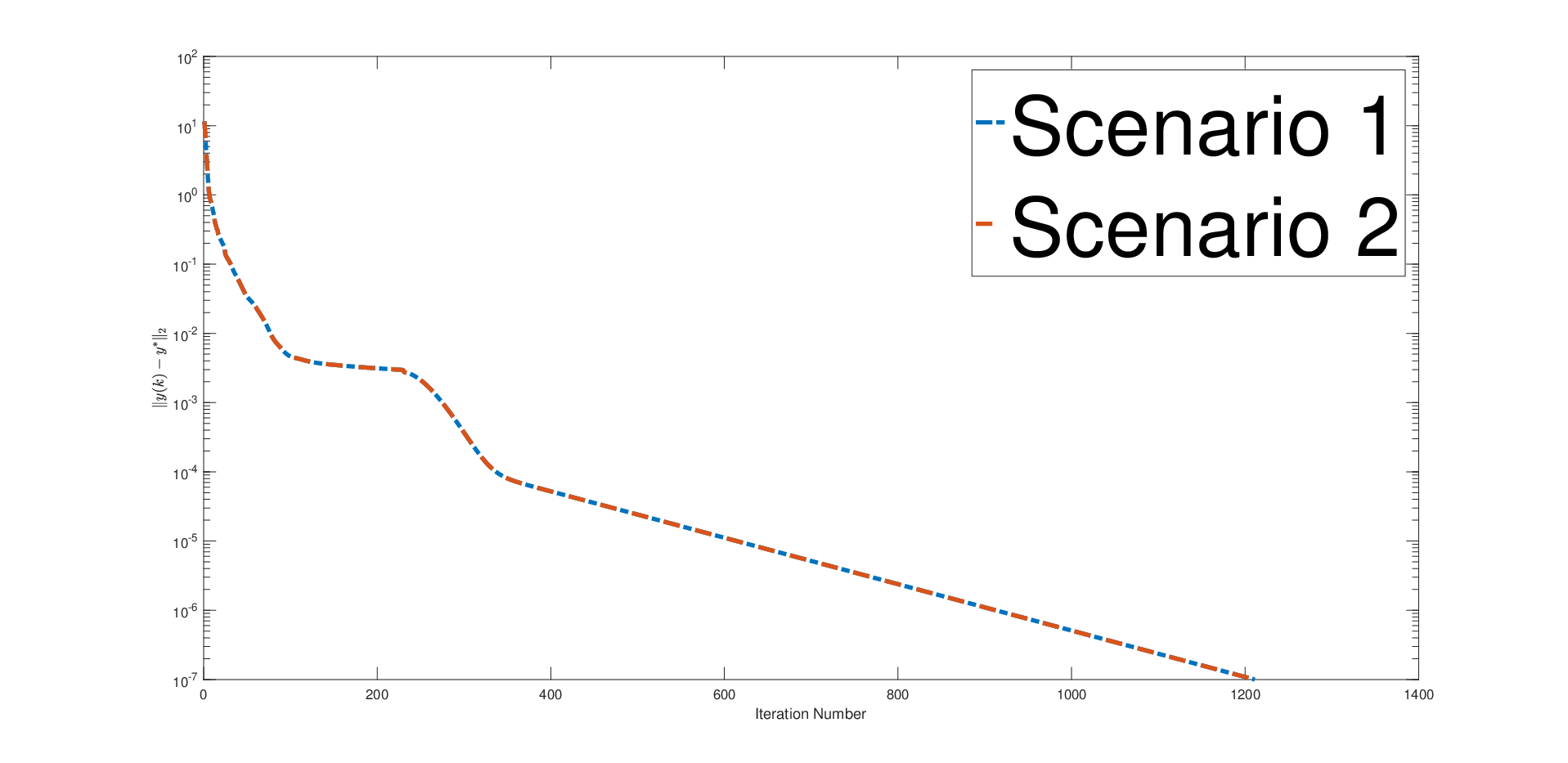
Refer to caption Refer to caption
Figure 2: Trajectories of ‖yk−y∗‖2\|y^{k}-y_{*}\|_{2} in the LASSO for 𝒞=ℝN\mathcal{C}=\mathbb{R}^{N} (using 10 logarithmic scale for the vertical axis and linear scale for the horizontal axis). Left: Stage one; Right: Stage two.

∙\bullet BPDN The parameter σ=0.2\sigma=0.2, and the regularization parameter in the second stage α=0.15\alpha=0.15. Further, ‖b‖2=2.9688\|b\|_{2}=2.9688 such that ‖b‖2>σ\|b\|_{2}>\sigma. When 𝒞=ℝN\mathcal{C}=\mathbb{R}^{N} (resp. 𝒞=ℝ+N\mathcal{C}=\mathbb{R}^{N}_{+}), the termination tolerances for the first and second stage are 10−710^{-7} (resp. 10−510^{-5}) and 8×10−48\times 10^{-4} (resp. 2×10−42\times 10^{-4}) respectively.

Constraint Jdist∗J^{*}_{\text{dist}} JREJ_{\text{RE}}
𝒞=ℝN\mathcal{C}=\mathbb{R}^{N} Scenario 1 1.0271 2.2×10−52.2\times 10^{-5}
Scenario 2 1.0209 5.9×10−35.9\times 10^{-3}
Constraint Jdist∗J^{*}_{\text{dist}} JREJ_{\text{RE}}
𝒞=ℝ+N\mathcal{C}=\mathbb{R}^{N}_{+} Scenario 1 1.1599 5.4×10−45.4\times 10^{-4}
Scenario 2 1.1607 1.3×10−31.3\times 10^{-3}

∙\bullet Fused LASSO The matrix E=[λ​Iγ​D1]E=\begin{bmatrix}\lambda I\\ \gamma D_{1}\end{bmatrix} with λ=0.6\lambda=0.6 and γ=0.4\gamma=0.4, and the regularization parameter α=0.18\alpha=0.18. For 𝒞=ℝN\mathcal{C}=\mathbb{R}^{N} and 𝒞=ℝ+N\mathcal{C}=\mathbb{R}^{N}_{+}, the termination tolerances for the first and second stages are 10−510^{-5} and 10−410^{-4}, respectively.

Constraint Jdist∗J^{*}_{\text{dist}} JREJ_{\text{RE}}
𝒞=ℝN\mathcal{C}=\mathbb{R}^{N} Scenario 1 1.2431 7.2×10−37.2\times 10^{-3}
Scenario 2 1.2376 2.8×10−32.8\times 10^{-3}
Constraint Jdist∗J^{*}_{\text{dist}} JREJ_{\text{RE}}
𝒞=ℝ+N\mathcal{C}=\mathbb{R}^{N}_{+} Scenario 1 1.4346 4.2×10−34.2\times 10^{-3}
Scenario 2 1.4474 1.3×10−21.3\times 10^{-2}

∙\bullet BPDN arising from Fused Problem Consider the BPDN-like problem: minx∈𝒞⁡‖E​x‖1\min_{x\in\mathcal{C}}\|Ex\|_{1} subject to ‖A​x−b‖2≤σ\|Ax-b\|_{2}\leq\sigma, where the matrix E=[λ​Iγ​D1]E=\begin{bmatrix}\lambda I\\ \gamma D_{1}\end{bmatrix} with λ=0.6\lambda=0.6 and γ=0.4\gamma=0.4, and the regularization parameter α=0.18\alpha=0.18. Further, σ=0.2\sigma=0.2 and ‖b‖2=2.9688\|b\|_{2}=2.9688. When 𝒞=ℝN\mathcal{C}=\mathbb{R}^{N} (resp. 𝒞=ℝ+N\mathcal{C}=\mathbb{R}^{N}_{+}), the termination tolerances for the first and second stages are 10−510^{-5} (resp. 10−410^{-4}) and 10−510^{-5} (resp. 10−510^{-5}) respectively.

Constraint Jdist∗J^{*}_{\text{dist}} JREJ_{\text{RE}}
𝒞=ℝN\mathcal{C}=\mathbb{R}^{N} Scenario 1 1.2823 6.5×10−36.5\times 10^{-3}
Scenario 2 1.2841 7.9×10−37.9\times 10^{-3}
Constraint Jdist∗J^{*}_{\text{dist}} JREJ_{\text{RE}}
𝒞=ℝ+N\mathcal{C}=\mathbb{R}^{N}_{+} Scenario 1 1.4815 4.9×10−44.9\times 10^{-4}
Scenario 2 1.4817 5.9×10−45.9\times 10^{-4}

∙\bullet Group LASSO Consider 𝒞=ℝN\mathcal{C}=\mathbb{R}^{N} and a cyclic graph with the penalty parameter λ=1.8\lambda=1.8, and the regularization parameter α=0.18\alpha=0.18. The termination tolerances for the first and second stages are 10−510^{-5} and 8×10−68\times 10^{-6}, respectively. The numerical tests show that Jdist∗=1.2208J^{*}_{\text{dist}}=1.2208 and JRE=9.8×10⁻⁴J_{\text{RE}}=9.8\times 10^{-4}.

The above results demonstrate the effectiveness of the proposed two-stage distributed algorithms.

8 Conclusions

In this paper, column partition based distributed schemes are developed for a class of densely coupled convex sparse optimization problems, including BP, LASSO, BPDN and their extensions. By leveraging duality theory, exact regularization techniques, and solution properties of the aforementioned problems, we develop dual based fully distributed schemes via column partition. Sensitivity results are used to establish overall convergence of the two-stage distributed schemes for LASSO, BPDN, and their extensions. The proposed schemes and techniques shed light on the development of column partition based distributed schemes for a broader class of densely coupled problems, which will be future research topics.

References

  • [1]
  • [2] A. Beck, and M. Teboulle. A fast iterative shrinkage-thresholding algorithm for linear inverse problems. SIAM Journal on Imaging Sciences, Vol. 2(1), pp. 183–202, 2009.
  • [3] D.P. Bertsekas. Nonlinear Programming. 2nd Edition, Athena Scientific, Belmont, MA, 1999.
  • [4] R. H. Byrd, G.M. Chin, J. Nocedal, and F. Oztoprak. A family of second-order methods for convex ℓ1\ell_{1}-regularized optimization. Mathematical Programming, Vol. 159(1-2), pp. 435–467, 2016.
  • [5] R.W. Cottle, J.-S. Pang, and R.E. Stone. The Linear Complementarity Problem, Academic Press Inc., Cambridge, 1992.
  • [6] D. Davis and W. Yin. A three-operator splitting scheme and its opitmization applications. Set-valued and Variational Analysis, Vol. 25(4), pp. 829–858, 2017.
  • [7] F. Facchinei and J.-S. Pang. Finite-Dimensional Variational Inequalities and Complementarity Problems. Volumes I and II, Springer-Verlag, 2003.
  • [8] M. P. Friedlander and P. Tseng. Exact regularization of convex programs. SIAM Journal on Optimization, Vol. 18(4), pp. 1326–1350, 2007.
  • [9] S. Foucart and H. Rauhut. A Mathematical Introduction to Compressive Sensing. Birkhäuser, Basel, 2013.
  • [10] M.S. Gowda and R. Sznajder. On the Lipschitzian properties of polyhedral multifunctions. Mathematical programming, Vol. 74(3), pp.267–278, 1996.
  • [11] J. Hu, Y. Xiao, and J. Liu. Distributed asynchronous algorithms for solving locally coupled optimization problems on agent networks. 2018 IEEE Conference on Decision and Control, pp. 2420–2425, 2018.
  • [12] S.J. Kim, K. Koh, S. Boyd, and D. Gorinevsky. ℓ1\ell_{1} trend filtering. SIAM Review, Vol. 51(2), pp. 339–360, 2009.
  • [13] M.J. Lai and W. Yin. Augmented ℓ1\ell_{1} and nuclear-norm models with a globally linearly convergent algorithm. SIAM Journal on Imaging Sciences, Vol. 6(2), pp. 1059–1091, 2013.
  • [14] X. Li, D. Sun, and K.C. Toh. A highly efficient semismooth Newton augmented Lagrangian method for solving Lasso problems. SIAM Journal on Optimization, 28(1), pp. 433–458, 2018.
  • [15] J. Liu, and S.J. Wright. Asynchronous stochastic coordinate descent: Parallelism and convergence properties. SIAM Journal on Optimization, Vol. 25(1), pp. 351–376, 2015.
  • [16] J. F. Mota, J.M. Xavier, P.M. Aguiar, and M. Puschel. Distributed basis pursuit. IEEE Transactions on Signal Processing, Vol. 60(4), pp. 1942–1956, 2011.
  • [17] S. Mousavi and J. Shen. Solution uniqueness of convex piecewise affine functions based optimization with applications to constrained ℓ1\ell_{1} minimization. ESAIM: Control, Optimisation and Calculus of Variations, Vol. 25, article 26, 2019. DOI: https://doi.org/10.1051/cocv/2018061.
  • [18] Z. Peng, M. Yan, and W. Yin. Parallel and distributed sparse optimization. In IEEE Asilomar Conference on Signals, Systems and Computers, pp. 659–646, November, 2013.
  • [19] R. T. Rockafellar. Convex Analysis. Princeton University Press, 1970.
  • [20] J. Shen and S. Mousavi. Least sparsity of pp-norm based optimization problems with p>1p>1. SIAM Journal on Optimization, Vol. 28(3), pp. 2721–21751, 2018.
  • [21] J. Shen and S. Mousavi. Exact support and vector recovery of constrained sparse vectors via constrained matching pursuit. Submitted, 2019. Also available at ArXiv preprint ArXiv:1903.07236.
  • [22] J. Shen and J.-S. Pang. Linear complementarity systems with singleton properties: non-Zenoness. Proceedings of the 2007 American Control Conference, pp. 2769–2774, New York, July, 2007.
  • [23] W. Shi, Q. Ling, G. Wu, and W. Yin. A proximal gradient algorithm for decentralized composite optimization. IEEE Transactions on Signal Processing, Vol. 63(22), pp. 6013–6023, 2015.
  • [24] N. Simon and R. Tibshirani. Standardization and the group Lasso penalty. Statistica Sinica, Vol. 22(3), pp. 983–1001, 2012.
  • [25] M. Sion. On general minimax theorems. Pacific Journal of Mathematics, Vol. 8(1), pp. 171–176, 1958.
  • [26] S.J. Wright, R.D. Nowak, and M.A. Figueiredo. Sparse reconstruction by separable approximation. IEEE Transactions on Signal Processing, Vol. 57(7), pp. 2479–2493, 2009.
  • [27] L. Xiao and S. Boyd. Fast linear iterations for distributed averaging. Systems & Control Letters, Vol. 53(1), pp. 65–78, 2004.
  • [28] W. Yin. Analysis and generalizations of the linearized Bregman method. SIAM Journal on Imaging Sciences, Vol. 3(4), pp. 856–877, 2010.
  • [29] K. Yuan, Q. Ling, and W. Yin. On the convergence of decentralized gradient descent. SIAM Journal on Optimization, Vol. 26(3), pp. 1835–1854, 2016.
  • [30] M. Yuan and Y. Lin. Model selection and estimation in regression with grouped variables. Journal of the Royal Statistical Society: Series B (Statistical Methodology), Vol.68(1), pp. 49–67, 2006.
  • [31] H. Zhang, W. Yin, and L. Cheng. Necessary and sufficient conditions of solution uniqueness in 1-norm minimization. Journal of Optimization Theory and Applications, Vol. 164(1), pp. 109–122, 2015.
  • [32]