Exploring galaxy colour in different environments of the cosmic web with SDSS2020Exploring galaxy colour in different environments of the cosmic web with SDSS–References
Abstract
We analyze a set of volume limited samples from the SDSS to study the dependence of galaxy colour on different environments of the cosmic web. We measure the local dimension of galaxies to determine the geometry of their embedding environments and find that filaments host a higher fraction of red galaxies than sheets at each luminosity. We repeat the analysis at a fixed density and recover the same trend which shows that galaxy colours depend on geometry of environments besides local density. At a fixed luminosity, the fraction of red galaxies in filaments and sheets increases with the extent of these environments. This suggests that the bigger structures have a larger baryon reservoir favouring higher accretion and larger stellar mass. We find that the mean colour of the red and blue populations are systematically higher in the environments with smaller local dimension and increases monotonically in all the environments with luminosity. We observe that the bimodal nature of the galaxy colour distribution persists in all environments and all luminosities, which suggests that the transformation from blue to red galaxy can occur in all environments.
Keywords:
methods: statistical - data analysis - galaxies: formation - evolution - cosmology: large scale structure of the Universe.1 Introduction
The present Universe is full of galaxies which come in various shape and size with different mass, luminosity, colour, star formation rate, metallicity and HI content. Understanding the galaxy properties and their evolution is an important goal of cosmology. The modern galaxy surveys (2dFGRS,Colless et al. 2001; SDSS, Strauss et al. 2002) reveal that the galaxies are distributed in the cosmic web (Bond et al. 1996) which is an interconnected weblike network comprising of different types of environments such as filaments, sheets, knots and voids. The galaxy properties vary across the different environments in the cosmic web. For example, the well known density-morphology relation reveals that the ellipticals are preferably found inside the dense groups and clusters whereas the spirals are intermittently distributed in the fields (Hubble 1936; Zwicky 1968; Oemler 1974; Dressler 1980; Goto et al. 2003). These findings are further supported by other studies with two-point correlation function (Willmer, da Costa, & Pellegrini 1998; Brown, Webstar, & Boyle 2000; Zehavi et al. 2005), genus statistics (Hoyle et al. 2002; Park et al. 2005) and filamentarity (Pandey & Bharadwaj 2005; Pandey & Bharadwaj 2006) of the galaxy distribution. It is now well known that many other galaxy properties are strongly sensitive to their environment (Davis & Geller 1976; Guzzo et al. 1997; Zehavi et al. 2002; Hogg et al. 2003; Blanton et al. 2003; Einasto, et al. 2003a; Kauffmann et al. 2004; Mouhcine et al. 2007; Koyama et al. 2013). The formation and evolution of galaxies are known to be driven by accretion, tidal interaction, merger and various other secular processes. These physical processes are largely determined by the environment of the galaxies. The environment thus play a central role in the formation and evolution of galaxies and the study of the environmental dependence of the galaxy properties provides crucial inputs to the theories of galaxy formation and evolution.
A number of studies have been carried out to understand the environmental dependence of galaxy colour. The galaxy colour distribution is well fit with a double Gaussian distribution (Balogh, et al. 2004) which can be used to divide the galaxies into red and blue populations. It has been shown that the blue galaxies reside preferentially in low-density regions whereas the red galaxies inhabit the high-density regions (Hogg, et al. 2004; Baldry, et al. 2004; Blanton, et al. 2005; Ball, Loveday & Brunner 2008). Park, et al. 2007 find that the galaxy colour is not sensitive to local density at fixed luminosity and morphology. Balogh, et al. 2004 show that when the luminosity is fixed, the fraction of galaxies in the red population is a strong function of local density. Cooper, et al. 2010 find a highly significant correlation between stellar age and environment at fixed stellar mass for the red galaxies. Bamford et al. 2009 find that the galaxy colour is highly sensitive to environment at a fixed stellar mass. They reported that irrespective of morphology, the high stellar mass galaxies are mostly red in all environments whereas the low stellar mass galaxies are mostly blue in low density environment and red in high density environment.
Most of these studies use the local density as a proxy for the environment. Different methods are often used to define the environment based on the scale being probed (Muldrew, et al. 2012). The various environments of the cosmic web are characterized by the density as well as their geometry. The clusters represent the densest regions in the cosmic web followed by the filaments, sheets and voids. The galaxy clusters are the dense knots which reside at the intersection of elongated filaments. The filaments in the cosmic web are located at the intersection of sheets which encompass large empty regions or voids. Studies with N-body simulations (Aragón-Calvo, et al. 2010; Cautun, et al. 2014; Ramachandra & Shandarin 2015) suggest that matter successively flows from voids to walls, walls to filaments and then channelled along the filaments onto the clusters. The dark matter halos formed at various environments of the cosmic web are known to have different mass, shape and spin due to the influence of their large-scale environment (Hahn et al. 2007). The galaxies are assumed to form at the centre of these dark matter halos via cooling and condensation of baryons (White & Rees 1978). In the halo model, the mass of the dark matter halo is believed to be the single most important parameter which determines the properties of a galaxy (Cooray & Sheth 2002). However the clustering of the dark matter halos depend on their assembly history (Croton, Gao & White 2007; Gao & White 2007; Musso, et al. 2018; Vakili & Hahn 2019) besides their mass. This implies that the environmental dependence of the galaxy properties may extend beyond the local density and the large-scale environments in the cosmic web may impart significant influence on the formation and evolution of galaxies. However there are no universal measure for characterizing the large-scale environments in the cosmic web. Some of the existing statistical tools designed for this purpose are the Shapefinders (Sahni et al. 1998), the statistics of maxima and saddle points (Colombi, Pogosyan & Souradeep 2000), the multiscale morphology filter (Aragón-Calvo et al. 2007), the skeleton formalism (Novikov et al. 2006) and the local dimension (Sarkar & Bharadwaj 2009).
In the present work, we use the local dimension (Sarkar & Bharadwaj 2009) to quantify the different environments in the cosmic web. A recent analysis with local dimension find that the sheets are the most prevalent pattern in the SDSS galaxy distribution which can extend up to (Sarkar & Pandey 2019). They also show that the straight filaments extend only up to a length scale of . The different structural components of the cosmic web differ in density, morphology and size. Each of these components provides an unique environment for galaxy formation and evolution. The role of the large-scale environment in this context is not yet settled. Luparello et al. 2015 find that the properties of the brightest group galaxies in the SDSS depend on their embedding large-scale structures. Using SDSS, Scudder et al. 2012 find that the star formation rates in isolated groups and the groups embedded in superstructures are significantly different. Yan, Fan & White 2013 analyze the SDSS data to find that the tidal environment of large scale structures do not influence the galaxy properties. Eardley, et al. 2015 studied the luminosity function in different environments using GAMA survey and find no evidence of the influence of environments beyond local density. Recently, Lee 2018 show that the elliptical galaxies in the sheetlike environment dwell in the regions with the highest tidal coherence. Pandey & Sarkar 2017 analyze the Galaxy Zoo (Lintott et al. 2008) data using information theoretic measures to find that morphology and environment exhibit a synergic interaction up to a length scales of .
The Sloan Digital Sky Survey (SDSS) is the largest spectroscopic and photometric galaxy redshift survey to date. It provides an unprecedented view of the cosmic web by precisely mapping millions of galaxies in the nearby Universe. In the present work, we analyze the spectroscopic data from the SDSS DR16 (Ahumada, et al. 2019). The primary aim of the present work is to identify the galaxies in different environments of the cosmic web using local dimension and explore the variations of red and blue galaxy fractions and their average colours across these environments. This would reveal how the galaxy colour is influenced by the different environments in the cosmic web. We study how the red and blue fractions vary in different geometric environments. We carry out the same analysis at a fixed local density to see if geometry of environments have any role in deciding the colours of galaxies. We also study the variations of red and blue fractions across different environments characterized by their local denisty. Besides density and geometry, the size of the different structural components of the cosmic web may also play a role in shaping the colour of a galaxy. We address this by measuring the red and blue fractions across different environments with increasing length scales keeping the luminosity of the galaxies fixed. We also study the bimodal nature of the colour distribution across different environments at different luminosities and examine how the mean and dispersion of galaxy colour are sensitive to these parameters. The analysis presented in this work would help us to understand the environmental factors besides the local density which may influence the colour of galaxies.
We use a CDM cosmological model with , and to calculate distances from redshifts throughout the analysis.
A brief outline of the paper is as follows. The method of analysis and the data are described in Section 2 and Section 3 respectively. The results of the analysis are discussed in Section 4 and we present our conclusions in Section 5.

2 METHOD OF ANALYSIS
We use the local dimension to isolate the galaxies residing in different geometric environments of the cosmic web. We count the number of galaxies within a sphere of radius centered on each galaxy. The radius of the sphere is varied within a specific range and the number counts are measured for a number of different radius at equally spaced interval of within this range. Only the galaxies for which all the spheres with radius in this range remain completely inside the survey boundary are treated as valid centres. For any volume limited galaxy sample this would be possible for only a subset of galaxies and the number of classifiable galaxies would decrease with increasing . In the present analysis we choose and then gradually increase in steps of up to the radius of the largest sphere that would fit inside the survey region.
The galaxies are embedded in different geometric environments in the cosmic web and the number count around a galaxy is expected to scale as,
| (1) |
where A is a constant and the exponent is the local dimension (Sarkar & Bharadwaj 2009). The local dimension tells us about the geometry of the embedding environment within a length scale range . We consider only the centres for which there is at least 10 galaxies within this radius range. For each centres, We obtain the best fit values of A and using the least-square fitting. We calculate the associated values using the observed and the fitted values of . Only the galaxies for which the chi-square per degree of freedom are considered in the present analysis. Ideally one would expect for galaxies residing in filaments, for the galaxies residing in sheets and for the galaxies residing in a three dimensional volume. However the size and shape of these structures vary considerably within the cosmic web. Besides there would be galaxies in the intermediate environments (e.g. junction of a sheet and a filament). In this case the measuring sphere would incorporate multiple type of structures within it. We classify the environment of a galaxy in five different classes (Table 1) depending on their local dimension. We assign a specific range of local dimension to each class. The galaxies in class are residing in filaments. These galaxies will primarily represent the middle parts of the straight filaments, which are not closer to the nodes. The -type galaxies may also represent short tendrils of galaxies which are found to link filaments together and penetrate into voids as coherrent structures (Alpaslan et al. 2014). The type galaxies are embedded in sheets. The type galaxies are mostly field galaxies in the low density regions. The type galaxies have intermediate local dimension between filaments and sheets whereas galaxies have local dimension in between sheets and fields. The environment of a galaxy as indicated by its local dimension would depend on the length scales under consideration.
We isolate the galaxies in different environments and segregate them into red and blue populations in each environment based on their colour. We use an optimal colour cut prescribed by Strateva, et al. 2001 to classify the red and blue galaxies. The galaxies with are identified as blue whereas the ones with are termed as red. We use the observed colour for simplicity keeping in mind the similar redshift range of the volume limited samples used in this work.
Red galaxies are known to reside in relatively denser environments. We also consider the effects of local density on the fraction of red and blue galaxies. We would like to test if the effects of environment extend beyond the local density and whether morphology of large scale structures play any role in deciding the colours of galaxies.
The local density at each galaxy position is estimated by using nearest neighbour method (Casertano & Hut 1985). In this method, the local number density is defined as,
| (2) |
where the nearest neighbour distance to the galaxy is and . We choose for the present analysis. We classify the galaxies into five different categories based on the local density at their locations. The criteria for each density class are provided in Table 3.
We calculate the fraction of red and blue galaxies in each geometric environment on different length scales for each of the volume limited samples described in the next section. We prepare 10 jackknife samples from each volume limited sample to estimate the errorbars for our measurements. Each jackknife sample is prepared by randomly deleting galaxies from the original sample.
| Local dimension : | |||||
|---|---|---|---|---|---|
| Classified as: |
| Volume | Absolute | Number of | Number | Mean inter-galactic | Radial | |
|---|---|---|---|---|---|---|
| limited | magnitude | Redshift () | galaxies | density | separation | size |
| samples | () | ( ) | () | () | ||
| Sample 1 | ||||||
| Sample 2 | ||||||
| Sample 3 |
| Local density class | |||||
|---|---|---|---|---|---|
| Local density range ( in ) |




| Sample | Total | Number of galaxies classified at | |||||
|---|---|---|---|---|---|---|---|
| Name | galaxies | ||||||
| Sample 1 | 90270 | ||||||
| Total: | 71634 | Total: | 29971 | Total: | 5089 | ||
| D1: | 6362 | D1: | 0 | D1: | 0 | ||
| D1.5: | 19229 | D1.5: | 951 | D1.5: | 0 | ||
| D2: | 21060 | D2: | 8464 | D2: | 497 | ||
| D2.5: | 13213 | D2.5: | 13037 | D2.5: | 3100 | ||
| D3: | 11770 | D3: | 7519 | D3: | 1492 | ||
| Sample 2 | 104137 | ||||||
| Total: | 82073 | Total: | 41820 | Total: | 15053 | ||
| D1: | 11167 | D1: | 25 | D1: | 0 | ||
| D1.5: | 23630 | D1.5: | 1483 | D1.5: | 90 | ||
| D2: | 22479 | D2: | 12972 | D2: | 1820 | ||
| D2.5: | 13207 | D2.5: | 17749 | D2.5: | 8370 | ||
| D3: | 11590 | D3: | 9591 | D3: | 4773 | ||
| Sample 3 | 92848 | ||||||
| Total: | 67673 | Total: | 43578 | Total: | 20212 | ||
| D1: | 12109 | D1: | 55 | D1: | 0 | ||
| D1.5: | 20717 | D1.5: | 2444 | D1.5: | 144 | ||
| D2: | 17177 | D2: | 15700 | D2: | 3999 | ||
| D2.5: | 9496 | D2.5: | 17519 | D2.5: | 11153 | ||
| D3: | 8174 | D3: | 7860 | D3: | 4916 | ||
| Sample | Number of D2 type galaxies which are common at | ||
|---|---|---|---|
| Name | and | , and | and |
| Sample 1 | 2812 | 181 | 411 |
| Sample 2 | 3352 | 568 | 1219 |
| Sample 3 | 3126 | 1084 | 2890 |


3 DATA
3.1 SDSS data
The Sloan Digital sky survey (SDSS) is a multi band imaging and spectroscopic redshift survey which covers more than one third of the celestial sphere. We use the Main galaxy sample for the present analysis. The spectroscopic target selection for the Main galaxy sample is described in Strauss et al. 2002. The photometric camera used in SDSS is described in Gunn et al. 1998. Fukugita et al. 1996 describe the photometric system used in the survey. The collection of data for the Main Galaxy sample was completed by SDSS DR7 (Abazajian et al. 2009). We use data from the data release (Ahumada, et al. 2019) of the Sloan Digital sky survey (SDSS). SDSS DR16 is the fourth and final data release of SDSS IV which incorporates data from all the prior data releases. We download the data from the SDSS SkyServer 11 1 https://skyserver.sdss.org/casjobs/ using Structured Query Language (SQL). For the present analysis, we select a contiguous region of the sky which spans and where and are the right ascension and declination respectively. We select all the galaxies with r-band Petrosian magnitude and redshift . These cuts provides us a total galaxies. We then construct three volume limited samples (Figure 1) by applying cuts to the K-corrected and extinction corrected -band absolute magnitude. The properties of these volume limited samples are described in detail in Table 2.
We apply the method described in the previous section to identify the galaxies in different environments in each of these volume limited samples. The exact number of galaxies classified in different classes at three different values of are tabulated in Table 4 for the three volume limited samples.
3.2 MultiDark simulation data
The three dimensional distribution of SDSS galaxies are obtained from their spectroscopic redshifts. The redshifts are perturbed by peculiar velocities of galaxies which distort their clustering pattern in redshift space (Kaiser 1987). We would like to quantify the effects of redshift space distortions on local dimension using mock samples from N-body simulations. We prepare a set of mock samples for the Sample 2 (Table 2) using data from the cosmosim project22 2 https://www.cosmosim.org/. The MultiDark Planck 2 (MDPL2) simulation is part of a number of simulations (Klypin, et al. 2016) based on cosmological parameters from Planck. The simulation is executed with dark matter particles in a cube of size , starting from redshift . The mass resolution of the simulation is . The values of the cosmological parameters used in the simulation are , , , , and . We have used the ROCKSTAR catalogue (Behroozi, Wechsler & Wu 2013) of MDPL2. We use a SQL query to retreive the position and velocities of the dark matter particles in snapshot 125 (). We place the observer at each corners of the cube and randomly select particles from each of these non-overlapping regions to prepare 8 mock samples which have exactly identical geometry as Sample 2. We prepare the mock samples both in real space and redshift space. The mock samples in redshift space are constructed by computing redshifts of galaxies from their distances in real-space and peculiar velocities. We analyze these mock samples in the same way as the actual data .
4 Results
4.1 Variations of environments with length scale
The different environments of the cosmic web have different characteristic size and their abundance would depend on the length scales probed. We first quantify the number of classifiable galaxies in each type of environment. The top three panels of Figure 2 show the number of classified galaxies in different types of environment as a function of length scale in Sample 1, Sample 2 and Sample 3. The respective fraction of galaxies available at each type of environment on each length scale for the three volume limited samples are shown in the bottom three panels of the same figure. We choose and then increase in uniform steps of starting from . The number of classifiable galaxies in each sample is expected to decrease with increasing due to their finite size.
In the bottom three panels of Figure 2, we find that the galaxies live in diverse environments on small scales. In each of the three volume limited samples, nearly galaxies reside in filaments and sheets when the environment is characterized within a length scale of . The type environments are mostly associated with the straight filaments which extend only up to in these samples. The galaxies which are part of the curved or warped filaments would be mostly represented by the type galaxies. We find that the type environment extends up to . The fraction of and type galaxies steadily decrease with increasing length scales. The type galaxies reside in sheets which are the most abundant environment within a scale of . The abundance of sheet peaks around in all three volume limited samples. The fraction of galaxies in sheetlike environment decreases with increasing length scales and only galaxies are part of sheetlike structures at . No galaxies are found to be a part of filamentary environment at this length scale. Comparison of the results from the three volume limited samples suggests that the filamentary and sheetlike environments can be traced to a slightly larger length scales in the brighter samples. This results from the larger number of classifiable galaxies available at larger length scales due to the bigger volumes of the brighter samples. At , of the galaxies are part of and type environments which indicates that the diversity of environment ceases to exist on larger length scales. The fact that the local dimension of galaxies shift towards hints towards the emergence of a homogeneous network of galaxies on sufficiently large length scales. This is consistent with the findings of various studies on large-scale homogeneity which suggests that the Universe is statistically homogeneous on scales beyond (Yadav et al. 2005; Hogg et al. 2005; Sarkar et al. 2009; Scrimgeour et al. 2012; Nadathur 2013; Pandey & Sarkar 2015; Pandey & Sarkar 2016; Avila et al. 2018). In Figure 3, we separately show the distributions of , and type galaxies within a cube of side . The left panel of Figure 3 shows that type galaxies mostly reside in short and straight filaments. The middle panel shows that type galaxies occupy sheetlike environments which are visually most prominent. The distribution of type galaxies in the right panel is nearly homogeneous in nature.
4.2 Effects of redshift space distortions on local dimension
We analyze mock SDSS samples from the MultiDark simulations in real space and redshift space to quantify the effects of redshift space distortions on local dimension. We compute the fraction of , and type galaxies in the mock SDSS samples as a function of length scale in real space and redshift space. Only a small fraction of galaxies are found to reside in type environments in these mock samples. So we do not show the results for type galaxies here. We compare the results in real space and redshift space in each case. The results are shown in Figure 4. The left, middle and right panel of Figure 4 respectively show the fraction of , and type galaxies as a function of length scale in real and redshift space. The results in redshift space are qualitatively similar to what we observe for SDSS galaxies in Figure 2. The left panel of this figure suggests that there is a marginal decrease in the fraction of type galaxies in redshift space. The same trend is also observed for type galaxies. This result is somewhat counter intuitive as one would expect an enhancement of short filaments in redshift space due to the ‘Finger of God’(FOG) effect. The ‘FOG’ stretches the dense virialized groups along the line of sight which are expected to resemble short filaments. However, we do not observe any such trend with or type galaxies in our mock SDSS sample. This may happen if the analyzed sample do not contain sufficient virialized dense groups in it. Some of the short filaments with orientations other than parallel and perpendicular to the line of sight in real space, may not be identified as filaments in redshift space, which causes a marginal decrease in their abundance. In the middle panel, there is a marginal increase in the fraction of type galaxies in redshift space on small scales. The trend reverses on large scales showing a small decrease in the fraction of type galaxies in redshift space. However, these differences are well within the error bars or very close to it. The right panel of Figure 4 shows that the fraction of type galaxies are least affected by redshift space distortions. We also repeat the same analysis with mock samples for Sample 3 and find analogous results. The test with the mock samples suggests that the redshift space distortions do not impart a statistically significant influence on the local dimension of galaxies and there are no preferred scale in the analysis.
4.3 Variations of red and blue fractions with geometric environment and length scale
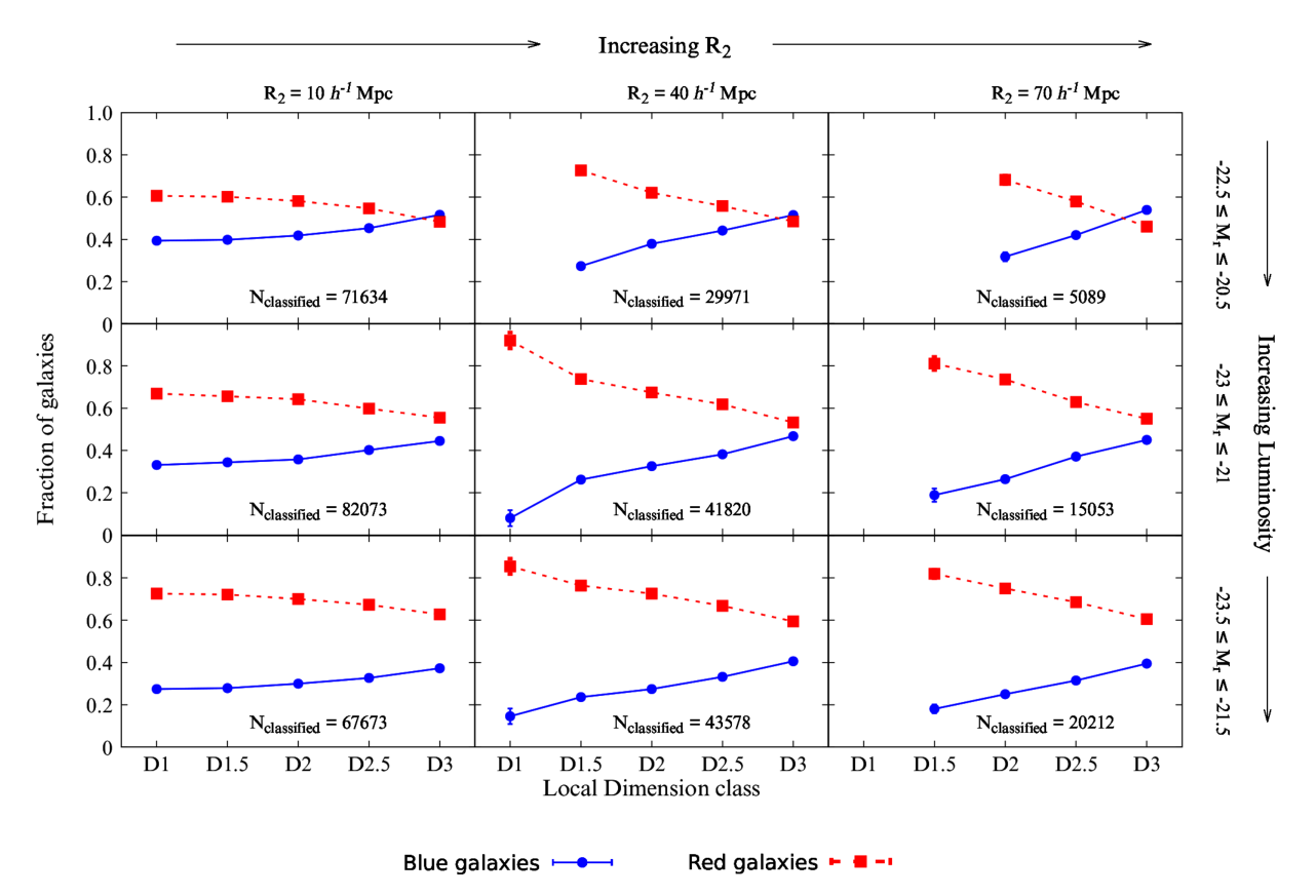
We show the fraction of red and blue galaxies in different environments of the cosmic web for Sample 1, Sample 2 and Sample 3 respectively in the top, middle and bottom panels of Figure 5. The left, middle and right panels at the top, middle and bottom row of Figure 5 corresponds to three different length scales , and respectively. Thus each row in Figure 5 corresponds to a fixed luminosity and each column corresponds to a a fixed length scale. The Figure 5 shows that environments with smaller local dimension tend to host a higher fraction of red galaxy. The red fraction at each local dimension increases when such environments are traced on larger length scales. There is also a clear increase in the red fraction at each environment with increasing luminosity. The luminosity dependence of red fraction is a well known phenomena. So we do not discuss the related results in greater detail. We only focus our attention on the dependence of red fraction on geometric environment and the length scales associated with such environment. We find that fraction of red galaxies dominates over the blue fraction at nearly each environment and each length scale. This is not necessarily true for all galaxy samples. We find that a reverse trend exists in fainter galaxy samples which are not included in this analysis. However, the decrease of red fraction with increasing local dimension is a common trend in all galaxy samples irrespective of their luminosity.
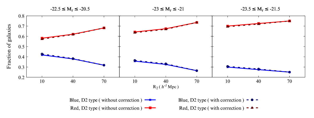
The Figure 5 shows that the fraction of red and blue galaxies also depends on the length scales associated with the environment. At a fixed luminosity and a fixed environment, the fraction of red galaxies increases with increasing length scales. We show the fraction of red and blue galaxies residing in sheets as a function of their size in the first 3 volume limited samples in Figure 6. The figure clearly shows that there is an increase in the fraction of red galaxies and a decrease in the fraction of blue galaxies with the increasing size of these structures. It is worthwhile to mention here that a subset of galaxies can be identified in the same type of environment on multiple length scales. These galaxies are part of such environment which extends at least up to the largest among these length scales. This must be taken into account while estimating the fraction of red or blue populations in different environments. We quantify the number of such galaxies at each environment for all the samples. For example, the number of such galaxies in type environment for different length scales are tabulated in Table 5. This table shows that in Sample 1, there are galaxies which reside in sheets at all three length scales i.e. , and . These galaxies are part of sheets extending to at least . Further, galaxies are part of sheets both at and but not at . These galaxies are part of sheets which are extended up to . We subtract these two numbers from the total number of galaxies identified in sheets on . Similarly, galaxies are identified in type environment both at and in Sample 1. The sheets associated with these galaxies extend at least up to . We subtract this number from the total number of galaxies found in sheets on a length scale of . The red and blue fractions in type environment are also corrected in Sample 2 and Sample 3 in a similar manner. We show both the corrected and the uncorrected fractions of red and blue galaxies in sheetlike environment at different length scales in Figure 6. We find that these corrections hardly make any difference to these results.
4.4 Comparing effects of density and geometry of environments on the red and blue fractions
Galaxy colour is known to be sensitive to local density. Generally sheets are denser than fields and filaments are denser than sheets. So the dependence of red and blue fractions on the geometry of large-scale environment shown in Figure 5 may partly arise due to dependence of galaxy colour on local density. We need to decorrelate the effect of local density in order to test the role of large scale structures on galaxy colours. We address this issue by calculating local number density of galaxies using nearest neighbour method (Casertano & Hut 1985). We compute the local number density using Equation 2 with . We plot the local density against the local dimension of galaxies in three different volume limited samples in Figure 7. The top left, middle left and bottom left panels of Figure 7 show the relations between local dimension and local density for the three volume limited samples when local dimensions are computed using . The results in these panels show that the environments with larger local dimension indeed tend to have a lower local density. However these relationships show very large scatters. The environments with local dimension up to can have a wide range of local densities and it is difficult to assign a specific density range to the environments with different local dimension. The three panels in the middle column and three panels in the right column of Figure 7 show the relations between local density and local dimension in these samples for and . They show a similar trend as seen in the three panels in the left column of the same figure. It may be noted that galaxies with smaller local dimension are progressively absent when the geometry of environments are characterized on larger length scales. This points out to the emergence of a homogeneous network of galaxies on larger length scales as mentioned earlier.
We first study the effect of local density on the red and blue fractions. We divide the galaxies into five different density classes based on their local density values. The different density classes are defined in Table 3. The left, middle and right panels of Figure 8 show the red and blue fractions of galaxies for different density classes in three volume limited samples. The left panel shows a clear increase in red fraction with increasing density. A higher fraction of red galaxies are observed for the brighter samples in the middle and right panels of Figure 8. However the density dependence are less pronounced in the brighter samples which indicates that the brighter galaxies are intrinsically redder irrespective of the density of their environments. This results may be related to the fact that brighter galaxies have higher stellar mass, which are mostly red in all environments (Bamford et al. 2009). Galaxies with lower luminosity have low stellar mass which are known to be blue in low density environment and red in high density environment. Our results are in good agreement with Bamford et al. 2009.
We then compare the red and blue fractions across the environments with different local dimension but at a fixed local density. Figure 7 shows that at , the lowermost density class has an uniform coverage of local dimension for all three volume limited samples. We consider all the galaxies in this density class and plot the red and blue fractions at different geometric environments for the three volume limited samples in Figure 9. Interestingly, the red fractions still show a mild decrease with increasing local dimension in each of the three panels of this figure. This suggests that geometry of environment also plays a role in deciding galaxy colour besides the local density. Unfortunately, we can not carry out this test for all density classes and all values due to non-uniform coverage (Figure 7).
This analysis indicates that both local density and geometry of environments play a role in deciding the colours of galaxies. The geometry and density dependence of red and blue fractions shown in Figure 5 and Figure 8 are most likely an outcome of the combined effects of density and geometry which are difficult to disentangle.
4.5 Bimodality of the colour distribution in different environments and luminosity
Galaxy colour is known to follow a bimodal distribution. We fit the distribution of the colour of galaxies using a double Gaussian with a PDF,
| (3) |
where and are the amplitudes of the two Gaussians. , are the associated weights, , are the means and , are the standard deviations of the two Gaussian components respectively. The usefulness of a double Gaussian fit in modelling galaxy colour distribution has been explored in a number of previous works (Balogh, et al. 2004; Baldry, et al. 2006). This approach has an inherent limitation due to the significant overlap of the two Gaussian distributions. A more rigorous approach to overcome this limitation is presented in Taylor, et al. 2015.
We plot the distributions of colour in different types of geometric environments on a length scale of for the three volume limited samples in different panels of Figure 10. We fit each of these distributions using a two Gaussian distribution (Equation 3). In each panel, the left and right peaks of the bimodal distribution corresponds to the blue and red galaxies respectively. We can clearly see that at each luminosity, the distribution of red galaxies are more sharply peaked than the blue galaxies in the geometric environments with smaller local dimension.
The mean and dispersion of the distributions at each geometric environment for the three volume limited samples are shown in Figure 11 and Figure 12 respectively. The Figure 11 shows that the mean colour of both the red and blue populations mildly decrease with increasing local dimension. At each geometric environment, the mean colour increases with increasing luminosity. We do not find a clear environmental trend for the dispersions in Figure 12. The dispersion for the red population is smaller than that for the blue population at each geometric environment. This is consistent with the visual impression from Figure 10 mentioned earlier. The dispersions for the red and blue populations at each geometric environment respectively increases and decreases with increasing luminosity.
The results of this analysis show that red galaxies prefer to reside in geometric environments with smaller local dimension. More luminous galaxies are found to be redder as expected. These findings are consistent with Figure 5 which show a similar dependence of the red and blue fraction on the local dimension and luminosity. Despite these variations across different environments and luminosities, the valley which separates the blue and red distributions appear around the same colour cut used to separate the two distributions. Finally, Figure 10 shows that the bimodal nature of the colour distribution is present across all environments and luminosities.
We could not repeat this analysis for and due to a relatively smaller number of galaxies available at these environments on those length scales.
5 CONCLUSIONS
We study the dependence of galaxy colour on different environments of the cosmic web using the data from SDSS DR16. We analyze a number of volume limited samples with different luminosity. We identify the galaxies in different environments by quantifying their local dimension on different length scales and estimate the fraction of red and blue galaxies in each environment for each of these samples. The analysis shows that for a fixed length scale, the fraction of red galaxies decreases with the increasing local dimension at each luminosity. At a fixed length scale, the fraction of red galaxies in each environment also increases with luminosity. The environments with lower values of local dimension are expected to represent denser regions of the cosmic web. Also the more luminous galaxies are known to be hosted in higher density regions (Einasto, et al. 2003b; Berlind, et al. 2005). These findings are consistent with the earlier studies on the environmental dependence of galaxy colour (Hogg, et al. 2004; Baldry, et al. 2004; Blanton, et al. 2005; Ball, Loveday & Brunner 2008; Bamford et al. 2009). The observed fraction of red galaxies thus depends on several interdependent parameters such as local density, geometry of environment and luminosity of galaxies. It is in general difficult to separate the role of these parameters in influencing colours of galaxies.
We separately study the dependence of red fractions on local density and find that the fraction of red galaxies increases with density. The trend persists across all the luminosity bins. The brighter samples host a higher fraction of red galaxies at the same density. At a fixed density, we study the fraction of red galaxies as a function of local dimension. This helps us to decorrelate the effect of density and test the effect of geometric environments on galaxy colours. We find that the fraction of red galaxies still decreases with increasing local dimension which suggests that geometry of environments also plays a role in determining the colours of galaxies. The effects of density and geometry are coupled due to their mutual correlation which is difficult to separate. A part of the density dependence of galaxy colours may arise due to geometry of their environment and vice versa.
The present analysis do not identify separate structures but only determine the geometric environment around a galaxy. We estimate the local dimension on various length scale ranges and consider only the best quality fits. So the estimated local dimension on a given length scale characterize the geometry of the environment of a galaxy on that length scale. We can not establish a direct relationship between the values and the size of the environment but it can be used as a proxy for their extent due to the involvement of the length scale in the fitting method for local dimension (Sarkar & Pandey 2019). At a fixed luminosity and a fixed local dimension, the fraction of red galaxies increases with . This indicates that the filaments and sheets which extends to larger length scales, host a higher fraction of red galaxies and a lower fraction of blue galaxies than their smaller counterparts. The relative change in the red fraction with the length scales is more pronounced in the fainter samples than the brighter samples. This is related to the fact that the effects of luminosity dominates in the brighter samples. The filaments and sheets extending to larger length scales are expected to have a larger baryon reservoir which must have started to form earlier (Zel’dovich 1970). These together would favour a higher accretion rate and a larger stellar mass for the galaxies in these environments. A higher accretion rate sustained for a longer period would exhaust the supply of gas in the surrounding environment leading to a higher fraction of red galaxies. It may be noted that a significant fraction of the red galaxies are known to be spirals (Masters, et al. 2010) which reside in filamentary and sheetlike environments of the cosmic web.
The distribution of galaxy colour in each environment can be described by a double Gaussian. We find that the mean colour of galaxies becomes redder with decreasing local dimension of the host environment and increasing luminosity of the sample. The dispersions of the red and blue distributions do not exhibit a clear trend with geometric environment. The results indicate that the environments with lower local dimension favour the transformation from blue to red galaxies. However the bimodal nature of the colour distribution persists in all environments which suggests that such transformations are allowed in all environments possibly via different physical mechanisms.
Finally, we would like to emphasize that the colour of a galaxy depends on the size of its host environment besides density and luminosity. The present analysis shows that the larger structures contain a higher fraction of red galaxies and a lower fraction of blue galaxies. Superclusters are known to have a sheetlike morphology with an intervening filamentary environment (Costa-Duarte, Sodré & Durret 2011; Einasto, et al. 2011; Einasto, et al. 2017). Einasto, et al. 2014 reported a higher fraction of red galaxies in filament-type superclusters. It would be also interesting to study the abundance and distribution of the red and blue galaxies in the individual superclusters of different size. Further, the recent studies with the Galaxy Zoo reveal that a large number of red galaxies are massive spirals (Bamford et al. 2009; Masters, et al. 2010; Tojeiro, et al. 2013). Masters, et al. 2010 find that the local density alone is not sufficient to explain the colour of these galaxies. They reported that the massive galaxies are red independent of their morphology.
The results of the present analysis suggests that if the massive red spirals are hosted in larger filaments or sheets then their colour may be explained by their embedding large-scale environment which favours a higher accretion rate leading to a larger stellar mass and consequently a faster depletion of the surrounding gas reservoir. In future, we plan to carry out such an analysis with the Galaxy Zoo which would help us to better understand the role of the embedding large-scale structures on the galaxy formation and evolution.
6 ACKNOWLEDGEMENT
The authors thank an anonymous reviewer for useful comments and suggestions which helped us to improve the draft. BP would like to acknowledge financial support from the SERB, DST, Government of India through the project CRG/2019/001110. BP would also like to acknowledge IUCAA, Pune for providing support through associateship programme. SS would like to thank UGC, Government of India for providing financial support through a Rajiv Gandhi National Fellowship. SS would also like to acknowledge Biswajit Das for useful discussions.
The authors would like to thank the SDSS team for making the data public. Funding for the Sloan Digital Sky Survey IV has been provided by the Alfred P. Sloan Foundation, the U.S. Department of Energy Office of Science, and the Participating Institutions. SDSS-IV acknowledges support and resources from the Center for High-Performance Computing at the University of Utah. The SDSS web site is www.sdss.org.
SDSS-IV is managed by the Astrophysical Research Consortium for the Participating Institutions of the SDSS Collaboration including the Brazilian Participation Group, the Carnegie Institution for Science, Carnegie Mellon University, the Chilean Participation Group, the French Participation Group, Harvard-Smithsonian Center for Astrophysics, Instituto de Astrofísica de Canarias, The Johns Hopkins University, Kavli Institute for the Physics and Mathematics of the Universe (IPMU) / University of Tokyo, the Korean Participation Group, Lawrence Berkeley National Laboratory, Leibniz Institut für Astrophysik Potsdam (AIP), Max-Planck-Institut für Astronomie (MPIA Heidelberg), Max-Planck-Institut für Astrophysik (MPA Garching), Max-Planck-Institut für Extraterrestrische Physik (MPE), National Astronomical Observatories of China, New Mexico State University, New York University, University of Notre Dame, Observatário Nacional / MCTI, The Ohio State University, Pennsylvania State University, Shanghai Astronomical Observatory, United Kingdom Participation Group, Universidad Nacional Autónoma de México, University of Arizona, University of Colorado Boulder, University of Oxford, University of Portsmouth, University of Utah, University of Virginia, University of Washington, University of Wisconsin, Vanderbilt University, and Yale University.
The CosmoSim database used in this paper is a service by the Leibniz-Institute for Astrophysics Potsdam (AIP). The MultiDark database was developed in cooperation with the Spanish MultiDark Consolider Project CSD2009-00064.
The authors gratefully acknowledge the Gauss Centre for Supercomputing e.V. (www.gauss-centre.eu) and the Partnership for Advanced Supercomputing in Europe (PRACE, www.prace-ri.eu) for funding the MultiDark simulation project by providing computing time on the GCS Supercomputer SuperMUC at Leibniz Supercomputing Centre (LRZ, www.lrz.de).
The Bolshoi simulations have been performed within the Bolshoi project of the University of California High-Performance AstroComputing Center (UC-HiPACC) and were run at the NASA Ames Research Center.
7 Data Availability
The data underlying this article are available in https://skyserver.sdss.org/casjobs/. The datasets were derived from sources in the public domain: https://www.sdss.org/
References
- Abazajian et al. (2009) Abazajian K. N., Adelman-McCarthy J. K., Agüeros M. A., Allam S. S., Allende Prieto C., An D., Anderson K. S. J., et al., 2009, ApJS, 182, 543
- Ahumada, et al. (2019) Ahumada R., et al., 2019, arXiv, arXiv:1912.02905
- Alpaslan et al. (2014) Alpaslan M., et al., 2014, MNRAS, 438, 177
- Aragón-Calvo et al. (2007) Aragón-Calvo, M. A., Jones, B. J. T., van de Weygaert, R., & van der Hulst, J. M. 2007, A&A, 474, 315
- Aragón-Calvo, et al. (2010) Aragón-Calvo M. A., Platen E., van de Weygaert R., Szalay A. S., 2010, ApJ, 723, 364
- Avila et al. (2018) Avila, F., Novaes, C. P., Bernui, A., & de Carvalho, E. 2018, JCAP, 12, 041
- Baldry, et al. (2004) Baldry I. K., Balogh M. L., Bower R., Glazebrook K., Nichol R. C., 2004, AIP Conference Proceedings, 743, 106
- Baldry, et al. (2006) Baldry I. K., Balogh M. L., Bower R. G., Glazebrook K., Nichol R. C., Bamford S. P., Budavari T., 2006, MNRAS, 373, 469
- Ball, Loveday & Brunner (2008) Ball N. M., Loveday J., Brunner R. J., 2008, MNRAS, 383, 907
- Balogh, et al. (2004) Balogh M. L., Baldry I. K., Nichol R., Miller C., Bower R., Glazebrook K., 2004, ApJL, 615, L101
- Bamford et al. (2009) Bamford, S. P., Nichol, R. C., Baldry, I. K., et al. 2009, MNRAS, 393, 1324
- Behroozi, Wechsler & Wu (2013) Behroozi P. S., Wechsler R. H., Wu H.-Y., 2013, ApJ, 762, 109
- Berlind, et al. (2005) Berlind A. A., Blanton M. R., Hogg D. W., Weinberg D. H., Davé R., Eisenstein D. J., Katz N., 2005, ApJ, 629, 625
- Blanton et al. (2003) Blanton, M. R., et al. 2003, ApJ, 594, 186
- Blanton, et al. (2005) Blanton M. R., Eisenstein D., Hogg D. W., Schlegel D. J., Brinkmann J., 2005, ApJ, 629, 143
- Brown, Webstar, & Boyle (2000) Brown, M.J.I., Webstar, R.L., & Boyle, B.J., 2000, MNRAS,317, 782
- Bond et al. (1996) Bond J. R., Kofman L., Pogosyan D. 1996, Nature, 380, 603
- Casertano & Hut (1985) Casertano S., Hut P., 1985, ApJ, 298, 80
- Cautun, et al. (2014) Cautun M., van de Weygaert R., Jones B. J. T., Frenk C. S., 2014, MNRAS, 441, 2923
- Colless et al. (2001) Colless, M. et al.(for 2dFGRS team) , 2001,MNRAS, 328, 1039
- Colombi, Pogosyan & Souradeep (2000) Colombi, S., Pogosyan, D., & Souradeep, T. 2000, PRL, 85, 5515
- Cooper, et al. (2010) Cooper M. C., Gallazzi A., Newman J. A., Yan R., 2010, MNRAS, 402, 1942
- Cooray & Sheth (2002) Corray, A., Sheth, R.K., 2002, Phys. Rep., 371, 1
- Costa-Duarte, Sodré & Durret (2011) Costa-Duarte M. V., Sodré L., Durret F., 2011, MNRAS, 411, 1716
- Croton, Gao & White (2007) Croton D. J., Gao L., White S. D. M., 2007, MNRAS, 374, 1303
- Dressler (1980) Dressler, A., 1980, ApJ, 236, 351
- Davis & Geller (1976) Davis, M., & Geller, M.J., 1976, ApJ, 208, 13
- Eardley, et al. (2015) Eardley E., et al., 2015, MNRAS, 448, 3665
- Einasto, et al. (2003a) Einasto, J., Hütsi, G., Einasto, M., Saar, E., Tucker, D. L., Müller, V., Heinämäki, P., & Allam, S. S. 2003, A&A, 405, 425
- Einasto, et al. (2003b) Einasto J., et al., 2003, A&A, 410, 425
- Einasto, et al. (2011) Einasto M., et al., 2011, ApJ, 736, 51
- Einasto, et al. (2014) Einasto M., Lietzen H., Tempel E., Gramann M., Liivamägi L. J., Einasto J., 2014, A&A, 562, A87
- Einasto, et al. (2017) Einasto M., et al., 2017, A&A, 603, A5
- Fukugita et al. (1996) Fukugita, M., Ichikawa, T., Gunn, J. E., Doi, M., Shimasaku, K., & Schneider, D. P. 1996, AJ, 111, 1748
- Gao & White (2007) Gao L., White S. D. M., 2007, MNRAS, 377, L5
- Goto et al. (2003) Goto, T., Yamauchi, C., Fujita, Y., Okamura, S., Seikiguchi, M., Smail, I. Bernardi, M., & Gomez, P.L., 2003, MNRAS, 346, 601
- Gunn et al. (1998) Gunn, J. E., et al. 1998, AJ, 116, 3040
- Guzzo et al. (1997) Guzzo, L., Strauss, M.A., Fisher, K.B., Giovanelli, R., & Haynes, M.P., 1997, ApJ, 489, 37
- Hahn et al. (2007) Hahn, O., Porciani, C., Carollo, C. M., & Dekel, A. 2007, MNRAS, 375, 489
- Hogg et al. (2003) Hogg, D. W., et al. 2003, ApJ Letters, 585, L5
- Hogg, et al. (2004) Hogg D. W., et al., 2004, ApJ Letters, 601, L29
- Hogg et al. (2005) Hogg, D. W., Eisenstein, D. J., Blanton, M. R., Bahcall, N. A., Brinkmann, J., Gunn, J. E., & Schneider, D. P. 2005, ApJ, 624, 54
- Hoyle et al. (2002) Hoyle, F., et al. 2002, ApJ, 580, 663
- Hubble (1936) Hubble, E.P., 1936, The Realm of the Nebulae (Oxford University Press: Oxford), 79
- Kaiser (1987) Kaiser, N. 1987, MNRAS, 227, 1
- Kauffmann et al. (2004) Kauffmann, G., White, S. D. M., Heckman, T. M., et al. 2004, MNRAS, 353, 713
- Klypin, et al. (2016) Klypin A., Yepes G., Gottlöber S., Prada F., Heß S., 2016, MNRAS, 457, 4340
- Koyama et al. (2013) Koyama, Y., Smail, I., Kurk, J., et al. 2013, MNRAS, 434, 423
- Lee (2018) Lee, J. 2018, ApJ, 867, 36
- Lintott et al. (2008) Lintott, C. J., Schawinski, K., Slosar, A., et al. 2008, MNRAS, 389, 1179
- Luparello et al. (2015) Luparello, H. E., Lares, M., Paz, D., et al. 2015, MNRAS, 448, 1483
- Masters, et al. (2010) Masters K. L., et al., 2010, MNRAS, 405, 783
- Mouhcine et al. (2007) Mouhcine, M., Baldry, I. K., & Bamford, S. P. 2007, MNRAS, 382, 801
- Muldrew, et al. (2012) Muldrew S. I., et al., 2012, MNRAS, 419, 2670
- Musso, et al. (2018) Musso M., Cadiou C., Pichon C., Codis S., Kraljic K., Dubois Y., 2018, MNRAS, 476, 4877
- Nadathur (2013) Nadathur, S. 2013, MNRAS, 434, 398
- Novikov et al. (2006) Novikov, D., Colombi, S., & Doré, O. 2006, MNRAS, 366, 1201
- Oemler (1974) Oemler A., 1974, ApJ, 194, 1
- Pandey & Bharadwaj (2005) Pandey, B. & Bharadwaj, S. 2005, MNRAS, 357, 1068
- Pandey & Bharadwaj (2006) Pandey, B., & Bharadwaj, S. 2006, MNRAS, 372, 827
- Pandey & Sarkar (2015) Pandey, B. & Sarkar, S. 2015, MNRAS, 454, 2647
- Pandey & Sarkar (2016) Pandey, B., & Sarkar, S. 2016, MNRAS, 460, 1519
- Pandey & Sarkar (2017) Pandey, B., & Sarkar, S. 2017, MNRAS, 467, L6
- Park et al. (2005) Park, C., et al. 2005, ApJ, 633, 11
- Park, et al. (2007) Park C., Choi Y.-Y., Vogeley M. S., Gott J. R., Blanton M. R., SDSS Collaboration, 2007, ApJ, 658, 898
- Ramachandra & Shandarin (2015) Ramachandra N. S., Shandarin S. F., 2015, MNRAS, 452, 1643
- Sahni et al. (1998) Sahni V., Satyaprakash B. S., & Shandarin S. F., 1998, ApJ, 495, L5
- Sarkar et al. (2009) Sarkar, P., Yadav, J., Pandey, B., & Bharadwaj, S. 2009, MNRAS, 399, L128
- Sarkar & Bharadwaj (2009) Sarkar, P., & Bharadwaj, S. 2009, MNRAS, 394, L66
- Sarkar & Pandey (2019) Sarkar S., Pandey B., 2019, MNRAS, 485, 4743
- Scrimgeour et al. (2012) Scrimgeour, M. I., Davis, T., Blake, C., et al. 2012, MNRAS, 3412
- Scudder et al. (2012) Scudder, J. M., Ellison, S. L., & Mendel, J. T. 2012, MNRAS, 423, 2690
- Strateva, et al. (2001) Strateva I., et al., 2001, AJ, 122, 1861
- Strauss et al. (2002) Strauss M. A., Weinberg D. H., Lupton R. H., Narayanan V. K., Annis J., Bernardi M., Blanton M., et al., 2002, AJ, 124, 1810
- Taylor, et al. (2015) Taylor E. N., et al., 2015, MNRAS, 446, 2144
- Tojeiro, et al. (2013) Tojeiro R., et al., 2013, MNRAS, 432, 359
- Vakili & Hahn (2019) Vakili M., Hahn C., 2019, ApJ, 872, 115
- White & Rees (1978) White, S. D. M., & Rees, M. J. 1978, MNRAS, 183, 341
- Willmer, da Costa, & Pellegrini (1998) Willmer, C.N.A., da Costa, L.N., & Pellegrini, P.S., 1998, AJ, 115, 869
- Yadav et al. (2005) Yadav, J., Bharadwaj, S., Pandey, B., & Seshadri, T. R. 2005, MNRAS, 364, 601
- Yan, Fan & White (2013) Yan, H., Fan, Z., White, S. D. M. 2013, MNRAS, 430, 3432
- York et al. (2000) York, D. G., et al. 2000, AJ, 120, 1579
- Zehavi et al. (2002) Zehavi, I., et al. 2002, ApJ,571,172
- Zehavi et al. (2005) Zehavi, I., et al. 2005, ApJ, 630, 1
- Zel’dovich (1970) Zel’dovich, Y. B. 1970, A&A, 5, 84
- Zwicky (1968) Zwicky, F., Herzog, E., Wild, P., Karpowicz, M., & Kowal, C., 1961-1968, Catalog of Galaxies and Clusters of Galaxies, vols. 1-6 (Pasadena: California Institute of Technology)