HOLISMOKES - I. Highly Optimised Lensing Investigations of Supernovae, Microlensing Objects, and Kinematics of Ellipticals and Spirals
Abstract
We present the HOLISMOKES programme on strong gravitational lensing of supernovae as a probe of supernova (SN) physics and cosmology. We investigate the effects of microlensing on early-phase SN Ia spectra using four different SN explosion models, and find that within 10 rest-frame days after SN explosion, distortions of SN Ia spectra due to microlensing are typically negligible (1% distortion within the 1 spread, and distortion within the 2 spread). This shows great prospects of using lensed SNe Ia to obtain intrinsic early-phase SN spectra for deciphering SN Ia progenitors. As a demonstration of the usefulness of lensed SNe Ia for cosmology, we simulate a sample of mock lensed SN Ia systems that are expected to have accurate and precise time-delay measurements in the era of the Rubin Observatory Legacy Survey of Space and Time (LSST). Adopting realistic yet conservative uncertainties on their time-delay distances and lens angular diameter distances (of 6.6% and 5%, respectively), we find that a sample of 20 lensed SNe Ia would allow a constraint on the Hubble constant () with 1.3% uncertainty in the flat CDM cosmology. We find a similar constraint on in an open CDM cosmology, while the constraint degrades to in a flat CDM cosmology. We anticipate lensed SNe to be an independent and powerful probe of SN physics and cosmology in the upcoming LSST era.
Key Words.
Gravitational lensing: strong – Gravitational lensing: micro – supernovae: general – Galaxies: distances and redshifts – Galaxies: kinematics and dynamics – cosmological parameters – distance scale1 Introduction
In the past few years, strongly lensed supernovae (SNe) have transformed from a theoretical fantasy to reality. First envisaged by Refsdal 1964 as a cosmological probe, a strongly lensed SN occurs when a massive object (e.g., a galaxy) by chance lies between the observer and the SN; the gravitational field of the massive foreground object acts like a lens and bends light from the background SN, so that multiple images of the SN appear around the foreground lensing object. The arrival times of the light rays of the multiple images are different, given the difference in their light paths. The time delays between the multiple SN images are typically days/weeks for galaxy-scale foreground lenses, and years for galaxy-cluster-scale foreground lenses. A strongly lensed SN is thus nature’s orchestrated cosmic fireworks with the same SN explosion appearing multiple times one after another. Refsdal 1964 showed that the time delays between the multiple SN images provide a way to measure the expansion rate of the Universe.
The first strongly lensed SN system with multiple resolved images of the SN was discovered by Kelly et al. 2015, half a century after the prescient Refsdal 1964. The SN was named “Supernova Refsdal”, and its spectroscopy revealed that it was a core-collapse SN (Kelly et al. 2016a). It was first detected serendipitously when it appeared in the galaxy cluster MACSJ1149.6+2223 in the Hubble Space Telescope (HST) imaging taken as part of the Grism Lens-Amplified Survey from Space (GLASS; PI: T. Treu) and the Hubble Frontier Field (PI: J. Lotz) programmes. While this was the first system that showed spatially-resolved multiple SN images, Quimby et al. 2013; Quimby et al. 2014 had previously detected a SN in the PanSTARRS11 1 Panoramic Survey Telescope and Rapid Response System survey (Kaiser et al. 2010; Chambers et al. 2016) that was magnified by a factor of by a foreground intervening galaxy, although the multiple images of the SN could not be resolved in the imaging. Two years after the SN Refsdal event was the first discovery of a strongly lensed Type Ia SN by Goobar et al. 2017 in the intermediate Palomar Transient Factory (Law et al. 2009), namely the iPTF16geu system. This is particularly exciting given the standardisable nature of Type Ia SNe for cosmological studies.
With strongly lensed SNe being discovered, we have new opportunities of using such systems to study SN physics, particularly SN progenitors. Strongly lensed SNe allow one to observe a SN explosion right from the beginning, which was impossible to do in the past given both the difficulty of finding SNe at very early phases and the time lag to arrange follow-up observations after a SN is detected. By exploiting the time delay between the multiple SN images, the lens system can be detected based on the first SN image and follow-up (especially spectroscopic) observations can be carried out on the next appearing SN image from its beginning. Early-phase observations are crucial for understanding the progenitors of SNe, especially Type Ia SNe whose progenitors are still a puzzle after decades of debate – are they single-degenerate (SD) systems with a white dwarf (WD) accreting mass from a nondegenerate companion and exploding when reaching the Chandrasekhar mass limit (Whelan & Iben 1973, e.g.,), or double-degenerate (DD) systems with two WDs merging (Tutukov & Yungelson 1981; Iben & Tutukov 1984, e.g.,), a mix of the two, or other mechanisms? A few SNe Ia now have extremely early light-curve coverage and a UV excess is observed in some of them (Dimitriadis et al. 2019, e.g.,), but there are no rest-frame UV spectra at such early phases to constrain the origin of the UV emission. A continuum-dominated UV flux would hint at shocks and interaction of the ejecta with a companion star or circumstellar matter, which would be prominent for 10% of the viewing angles, and would favour the SD scenario (Kasen 2010). A line-dominated early UV spectrum, on the other hand, would probe radioactive material close to the surface of the SN, as predicted by some DD models (Maeda et al. 2018).
Strongly lensed SNe with time-delay measurements also provide a direct and independent method to measure the expansion rate of the Universe, or the Hubble constant (), as first pointed out by Refsdal 1964. There is currently an intriguing tension in the measurements of from independent probes, particularly between the measurement from observations of the Cosmic Microwave Background (CMB) by the Planck Collaboration 2020 and the local measurement from Cepheids distance ladder by the “Supernovae, , for the Equation of State of Dark Energy” (SH0ES) programme (Riess et al. 2019). This tension, if not due to any unaccounted-for measurement uncertainties, has great implications for cosmology as it would require new physics beyond our current standard “flat CDM” cosmological model. The latest measurement from the Megamaser Cosmology Project by Pesce et al. 2020, which is independent of the CMB and SH0ES, corroborates the measurement of SH0ES, although it is within 3 of the Planck measurement. On the other hand, Freedman et al. 2019 measured that is right in between the values from Planck Collaboration 2020 and Riess et al. 2019 through the Carnegie-Chicago Hubble Program (Beaton et al. 2016, CCHP;) using a separate distance calibrator, the tip of the red giants, instead of Cepheids. There is ongoing debate about the method (Yuan et al. 2019; Freedman et al. 2020, e.g.,) and the results from CCHP and SH0ES are not fully independent due to calibrating sources/data that are common among the two distance ladders. Strong-lensing time delays are therefore highly valuable for providing a direct measurement, completely independent of the CMB, the distance ladder, and megamasers (Riess 2019).
Given the rarity of lensed SNe, the method of time-delay cosmography has matured in the past two decades using lensed quasars which are more abundant. The H0LiCOW (Suyu et al. 2017) and COSMOGRAIL (Courbin et al. 2018) collaborations have greatly refined this technique using high-quality data and state-of-the-art analyses of lensed quasars. The latest H0LiCOW measurement by Wong et al. 2020 from the analyses of 6 lens systems (Suyu et al. 2010; Suyu et al. 2014; Wong et al. 2017; Birrer et al. 2019; Jee et al. 2019; Chen et al. 2019; Rusu et al. 2020), which include 3 systems analysed jointly with the SHARP collaboration (Chen et al. 2019), is consistent with the results from SH0ES and is higher than the value from the Planck Collaboration 2020, strengthening the argument for new physics. Analysis of new lensed quasars is underway (e.g., Shajib et al. 2020, from the STRIDES collaboration), and a detailed account of systematic uncertainties in such measurements is presented by Millon et al. 2020 under the new TDCOSMO organisation. With time-delay cosmography maturing through lensed quasar, lensed SNe are expected to be a powerful cosmological probe.
The two known lensed SN systems, iPTF16geu and SN Refsdal, do not have early-phase spectroscopic observations for progenitor studies, and have yet to yield measurements. The time delays between the four SN images in iPTF16geu are short, day (More et al. 2017; Dhawan et al. 2019), and all four SN images were past the early phase when the system was discovered by Goobar et al. 2017. The short delays also make it difficult to obtain precise from this system, since the relative uncertainties in the delays (Dhawan et al. 2019, which are ;) sets the lower limit on the relative uncertainty on . On the other hand, SN Refsdal has one long time delay between the SN images (Treu et al. 2016; Grillo et al. 2016; Kawamata et al. 2016, year;), in addition to shorter delay pairs (Rodney et al. 2016). The reappearance of the long-delayed SN Refsdal image was detected by Kelly et al. 2016b, providing an approximate time-delay measurement. The precise measurement of the long delay using multiple techniques is forthcoming (P. Kelly, priv. comm.), and this spectacular cluster lens system with multiple sources at different redshifts could yield the first measurement from a lensed SN (Grillo et al. 2018; Grillo et al. 2020, e.g.,).
Even though lensed SNe are very rare, their numbers will increase dramatically in the coming years thanks to dedicated wide-field cadenced imaging surveys. In particular, Goldstein et al. 2019 forecasted about a dozen lensed SNe from the ongoing Zwicky Transient Facility (Bellm et al. 2019; Masci et al. 2019, ZTF;); most of these lensed SNe will be systems with short time delays (days) and high magnifications, given the bright flux limit of the ZTF survey. The upcoming Rubin Observatory Legacy Survey of Space and Time (Ivezić et al. 2019, LSST;)22 2 LSST is previously known as the Large Synoptic Survey Telescope. that will image the entire southern sky repeatedly for 10 years will yield hundreds of lensed SNe (Oguri & Marshall 2010; Goldstein et al. 2019; Wojtak et al. 2019, e.g.,). The efficiency of detecting these systems and measuring their time delays depends significantly on the observing cadence strategy. Huber et al. 2019 have carried out the first investigations of detecting lensed SNe Ia and measuring their delays in the presence of microlensing, with results that favour long cumulative season length and higher cadence.
With the upcoming boom in strongly lensed SNe, we initiate the HOLISMOKES programme: Highly Optimised Lensing Investigations of Supernovae, Microlensing Objects, and Kinematics of Ellipticals and Spirals. We are developing ways to find lensed SNe (Cañameras et al. 2020, HOLISMOKES II) in current/future cadenced surveys and to model the lens systems rapidly for scheduling observational follow-up (Schuldt et al. 2020, HOLISMOKES IV). We are also exploring in more detail the microlensing of lensed SNe Ia (Huber et al. 2020, HOLISMOKES III) and core-collapse SNe (Bayer et al. in prep., HOLISMOKES V) for measuring the time delays, following the works of Goldstein et al. 2018 and Huber et al. 2019.
In this first paper of the HOLISMOKES series, we study and forecast our ability to achieve two scientific goals with a sample of lenses from the upcoming LSST: constrain SN Ia progenitors through early-phase observations, and probe cosmology through lensing time delays. In Section 2, we investigate microlensing effects on SNe Ia to determine whether it is feasible to extract the intrinsic early-phase SN spectra that are crucial for revealing SN Ia progenitors. In Section 3, we forecast the cosmological constraints based on an expected sample of lensed SNe from LSST. We summarize in Section 4.
2 Microlensing of SNe Ia in their early phases
Early-phase spectra (within rest-frame days after explosion) carry valuable information to distinguish between different SN Ia progenitors (Kasen 2010; Rabinak & Waxman 2011; Piro & Nakar 2013; Piro & Nakar 2014; Piro & Morozova 2016; Noebauer et al. 2017, e.g.,). Problems arise when SNe are significantly influenced by microlensing (Yahalomi et al. 2017; Goldstein et al. 2018; Foxley-Marrable et al. 2018; Bonvin et al. 2019b; Huber et al. 2019), which distorts light curves and spectra, and therefore makes them hard to use as a probe for SN Ia progenitors. However, investigations by Goldstein et al. 2018 and Huber et al. 2019 show that microlensing of lensed SNe Ia is stronger in late phases than shortly after explosion. These results raise the hope to use lensed SNe Ia for the progenitor problem and motivates further investigation of the influence of microlensing on early-phase spectra.
In Section 2.1, we describe four explosion models for different SN progenitor scenarios from the ARTIS simulations (Kromer & Sim 2009) that we use. We then outline the microlensing formalism in Section 2.2, before presenting our results on the microlensed SN Ia spectra in Section 2.3.
2.1 SN Ia models from ARTIS simulations
To probe the effect of microlensing on SNe Ia, we need the time, wavelength, and spatial dependency of the SN radiation. For this, we consider four theoretical explosion models where synthetic observables have been calculated via ARTIS (Kromer & Sim 2009). We briefly describe these models below, and refer the readers to, e.g., Noebauer et al. 2017 for more details. These models allow us to explore various progenitor scenarios.
-
W7 (carbon deflagration):
The W7 model (Nomoto et al. 1984) is considered one of the benchmark theoretical models for the explosion of a carbon-oxygen (CO) white dwarf (WD) at the Chandrasekhar mass limit since it reproduces key observable features of SNe Ia. W7 is however not a self-consistent explosion model, in contrast to the other three models described below. The ARTIS spectral calculations for the W7 model is presented in Kromer & Sim 2009, and we use here the calculations with 7 ionisation stages. -
N100 (delayed detonation):
Following Röpke et al. 2012, the CO WD in this model has 100 randomly distributed ignition spots that trigger an initial subsonic deflagration, which then transitions into a detonation. For more details on the ARTIS spectral calculations, see Sim et al. 2013. -
subCh (sub-Chandrasekhar mass detonation):
This model is a centrally ignited detonation of a 1.06 CO WD (Sim et al. 2010, model 1.06 of). -
merger:
Following Pakmor et al. 2012, this model is a violent merger of a 0.9 and a 1.1 CO WD, triggering a carbon detonation in the 1.1 CO WD and disrupting the system.
We spherically average the photon packets from these simulations in order to obtain high signal-to-noise spatial and energy distributions of the photons from the SN Ia models. This is valid for W7 and subCh models that are spherically symmetric, and also a good approximation for the N100 model which shows minimal large-scale asymmetry (Röpke et al. 2012) and low continuum polarisation of 0.1% (Bulla et al. 2016). While the merger model is inherently non-spherically symmetric, we find the spherical averaging to be a good approximation; by following Huber et al. 2020 in separating portions of the photon packets of the merger model, we find that different portions of the photon packets yield similar results and our conclusions thus do not depend on asymmetries in the merger model.
In Figure 1, we show the rest-frame spectral evolution computed from ARTIS for the four different explosion models. Each column corresponds to a particular model as labelled on the top, and each row is for a rest-frame time after explosion as indicated on the right. The spectra at 4.0, 6.6 and 8.4 days are significantly different amongst the models, whereas the spectra at 20.7 and 39.8 days are more similar to each other in having iron-line blanketing in the UV and relatively strong absorption lines. In particular, at 4.0 days, W7 has weaker absorption lines especially in the optical and strong emission lines, whereas N100 and subCh have strong Ca II absorption lines. W7, N100 and subCh are brighter in the UV relative to the optical, whereas merger is not. At 6.6 and 8.4 days, N100 has more suppression in flux at wavelengths relative to the optical due to blended groups of Fe II, Ni II and Mg II absorption lines, whereas W7 and subCh continue to be bright in the UV and merger begins to have more UV flux relative to the optical.
While Figure 1 displays different relative fluxes in the UV to optical and different strengths of the absorption features in the early SN phases amongst the explosion models, we caution that the exact spectral shapes of these models depend on the various approximations used in the radiative transfer calculations (Dessart et al. 2014; Noebauer et al. 2017, e.g.,). In particular, the number of ionisation states and metallicity of the progenitor could affect particularly the UV spectra at levels comparable to the differences depicted in Figure 1 (Lucy 1999; Kromer & Sim 2009; Lentz et al. 2000; Kromer et al. 2016; Walker et al. 2012, e.g.,). Furthermore, these spectra do not include thermal radiations from possible interactions of the SN ejecta with a non-degenerate companion or with circumstellar matter. Such thermal radiation would only be in the very early phase within days though (Kasen 2010, e.g.,), so distinguishing spectral features after 4 days could still be used as diagnostics. Therefore, first acquisitions of the early-phase UV spectra would be extremely useful for providing clues to the explosion/progenitor scenarios, and for guiding future directions of model developments. Lensed SNe have a further advantage in that the SN are magnified by the lensing effect, typically by a factor of 10 for lensing galaxies and even 100 for lensing galaxy clusters, which facilitates spectroscopic observations33 3 The absolute rest-frame B-band magnitude of a SN Ia at peak is . For a SN at redshift 0.5, this corresponds to an apparent magnitude of 23 without lensing magnifications. A lensing magnification by a factor of 10 would brighten the apparent magnitude to 20.5..

2.2 Microlensing formalism and maps
We assume that microlensing maps and positions in the map do not vary over typical time scales of a SN Ia and the microlensing effect is therefore just related to the spatial expansion of the SN. This approach is motivated by the work of Goldstein et al. 2018 and Huber et al. 2019. We follow closely the formalism described in Huber et al. 2019 to compute microlensing effects on a SN Ia, and briefly summarise the procedure. The observed microlensed flux of a SN at redshift and luminosity distance can be determined via
| (1) |
where the emitted specific intensity , is multiplied with the microlensing magnification map44 4 Note that denotes the magnification factor and not as usually in radiative transfer equations. from GERLUMPH (Vernardos et al. 2015; Chan et al. 2020) and integrated over the whole size of the projected SN Ia. The specific intensity depends on the time since explosion , the wavelength , and the radial coordinate on the source plane , given our spherical averaging of the photon packets from the models55 5 In equation (1) the specific intensity is mapped onto a Cartesian grid (, ) to combine it with the magnification maps . For more details, see Huber et al. 2019.. The specific intensity profiles for different times after explosion are shown in Appendix A. Equation (1) is derived and explained in Huber et al. 2019. We refer readers to Huber et al. 2019 for an example showing the effects of microlensing on spectra and light curves in detail.
For this work we focus on the spectra, particularly at early phases. We investigate 30 different magnification maps. These maps depend on three main parameters: the lensing convergence , the shear , and the smooth matter fraction , where is the convergence of the stellar component. In our analysis we probe (, where we test for each combination of and the smooth matter fractions of . Six of these magnification maps are shown in Appendix B, where we explain also further inputs for producing the magnification maps. The values for the convergence and shear are calculated from the mock lens catalog of Oguri & Marshall 2010, taking into account 416 lensed SNe Ia that adopted a singular isothermal ellipsoid (Kormann et al. 1994) as lens mass model. The two pairs and correspond to the median values for type I lensing images (time-delay minimum) and type II images (time-delay saddle), respectively. The other pairs are the 16th and 84th percentiles of the OM10 sample, taken separately for and .
2.3 Spectral distortions due to microlensing


For each of the 30 magnification maps, we draw 10,000 random positions in the map to quantify the effect of microlensing on the SN spectra. For each position we calculate the microlensed flux via equation (1) and compare it to the case without microlensing () of a given SN Ia model. From this, we can calculate the deviation from the macro magnification as:
| (2) |
where is the normalised flux over a given wavelength range such that the integrated flux over the wavelength range yields the same sum for both the microlensed and the non-microlensed spectra (i.e., , and the normalisation constant is set such that ). The deviation quantifies distortions in the spectra of a microlensed SN relative to the intrinsic SN without microlensing, i.e., a deviation of 0 across all wavelengths implies no chromatic microlensing distortion on the intrinsic SN spectra. We note that a constant (macro)magnification across all wavelengths from macrolensing without microlensing yields also a deviation of 0, since is then the macrolensing magnification (a constant that is independent of wavelength) and after normalisation. We refer readers to Figures A.1 and A.3 of Huber et al. 2019 for examples of , which is up to a constant factor. From the 30 10,000 random configurations, we determine the median deviation of with the 1 range (68% interval, from the 16 percentile to the 84 percentile of the microlensed spectra) and 2 range (95% interval, from the 2.5 percentile to the 97.5 percentile).
We show the deviations at different times after explosions for the W7, N100, subCh and merger models in Figures 2 to 5, respectively. The median deviation (dashed black lines) is zero within for all models, indicating that the microlensing effect does not induce a systematic distortion on the spectra overall, even though each microlensed spectrum can indeed be distorted as shown by the 2 spreads. We find that at early times (within 10 rest-frame days after explosion), the 2 spread of for most wavelength regions is well within the level, especially for the W7 and merger models. In the N100 and subCh models, deviations in the UV can reach up to due to absorption features and suppression of UV flux in their spectra (see Figure 1). The insets in each of the panels clearly show that the 1 spread of for all SN models is within in the early phases (rest-frame days). Therefore, microlensing would not distort the spectra of SNe beyond at any wavelength in 68% of all strongly lensed SNe Ia at early phases. At later times ( 20 to 40 days), the influence of microlensing becomes substantially larger, as also visible in the increased 1 spread, but the 1 spread is still mostly below the level.
We find that deviations due to microlensing tend to be larger at wavelengths where the relative flux is low in the spectra, either due to absorption features or low-level continuum (as illustrated in Figures 1 to 5). This is because microlensing distorts spectra across all wavelengths, so wavelengths that have lower fluxes would have relatively larger variations in fluxes due to microlensing, and thus higher deviations, after normalising the spectra in equation (2). We refer the reader to Appendix C for an example of the covariance matrix of the deviations which further illustrates this.
The overall trend for all four SN models shows that both the 1 and 2 spreads are increasing over time. There are two reasons for this. The first reason is that the specific intensity profiles for different filters deviate more strongly from each other at later phases (Goldstein et al. 2018; Huber et al. 2019, and Appendix A), which leads to higher deviations in the spectrum between different wavelength regions. The second reason is that SNe Ia are expanding over time and therefore it is much more likely to cross a micro caustic at later times. Consequently, the effect of microlensing should be lower at the earliest phases ( days) compared to the first epoch from our simulations at days; SNe Ia have smaller sizes and thus smaller chances to be chromatically microlensed in these earliest phases.
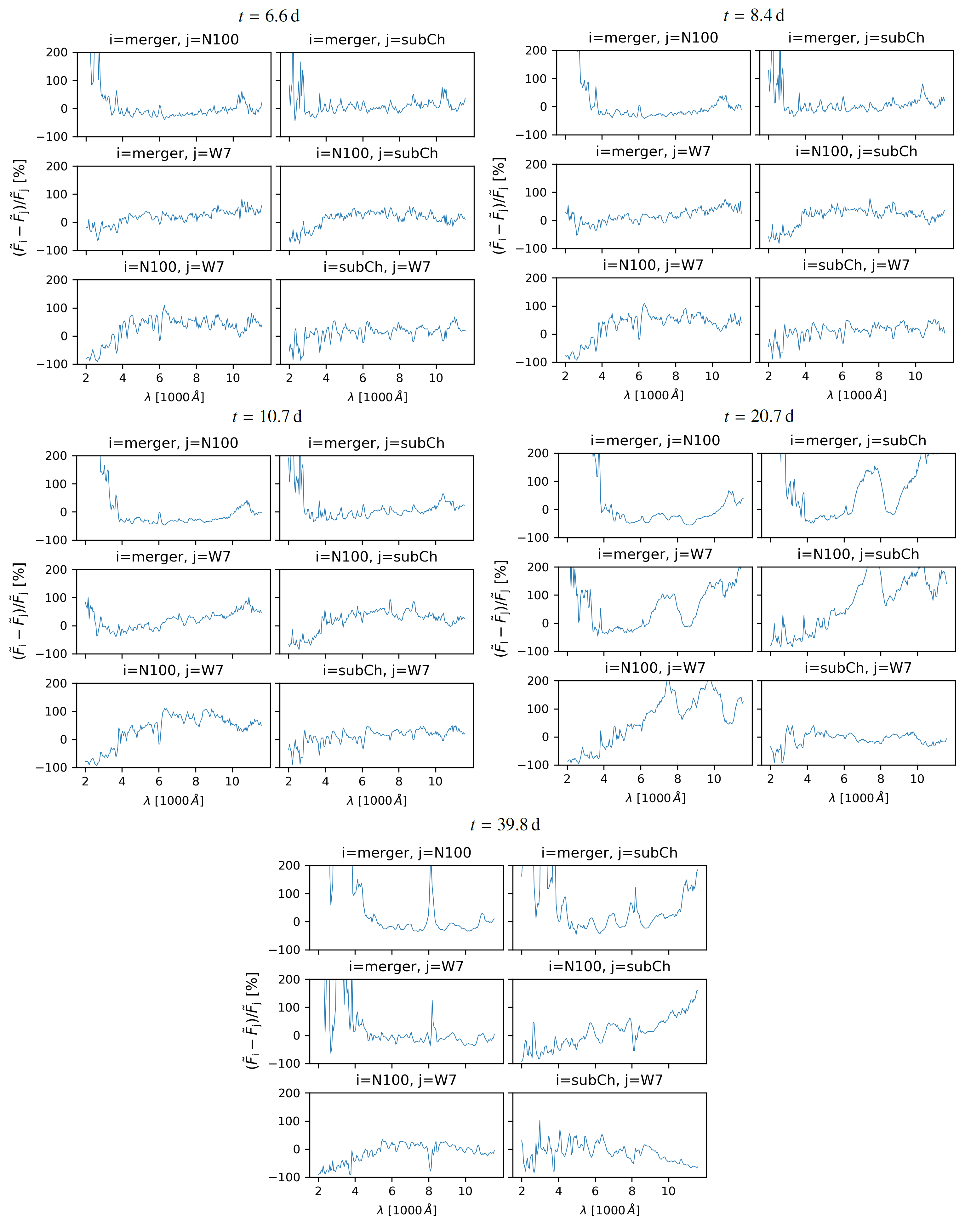
To assess the impact of microlensing on our ability to distinguish between SN explosion models from early-phase spectra, particularly in the UV wavelengths, we compare the deviations due to microlensing to the deviations due to model differences. In Figure 6, we show the deviations (equation 2) between all 6 possible pairs of the four SN Ia models we considered at rest-frame days after explosion. In the UV-wavelength range that is useful for progenitor studies (Section 2.1), the deviations are typically , which is an order of magnitude larger than the deviations due to microlensing shown in Figures 2 to 5, respectively. At later times, the deviations between the spectra from different models are shown in Appendix D, and continue to have high amplitudes. Therefore, deviations in the spectra due to microlensing are negligible compared to the deviations in the spectra arising from different SN Ia progenitor scenarios and from uncertainties in the spectra due to approximations in radiative transfer calculations.
To summarise, at early times ( rest-frame days) we have very good prospects to collect good quality spectra with negligible distortions from microlensing, which is necessary to address the SN Ia progenitor problem. Nevertheless, we would like to point out that there are extreme cases where microlensing can significantly influence even very early spectra. These extreme microlensing cases could potentially allow one to probe the specific intensity distribution of SNe. A comparison showing the dependency of microlensing effects on different parameters, such as , is presented in Huber et al. 2020, but especially for high magnification cases with both values of and close to 0.5, we find that chromatic microlensing distortion is more likely. This can be understood by looking at the magnification maps shown in Appendix B, where more caustics and higher gradients exist for and in comparison to the other cases. Fortunately, in practice we can always estimate for a given lensed SN Ia image the likelihood of it being microlensed, to determine whether it is suitable for obtaining a “clean” SN spectrum that has little distortion from microlensing.
3 Forecasted cosmological constraints from strongly lensed SNe
Each lensed SN provides an opportunity to measure two distances: the time-delay distance and the angular diameter distance to the deflector/lens (Refsdal 1964; Suyu et al. 2010; Paraficz & Hjorth 2009; Birrer et al. 2016; Jee et al. 2019, e.g.,). The time-delay distance is defined by Suyu et al. 2010 as
| (3) |
where and are angular diameter distances to the source from the deflector and from the observer, respectively. Measuring requires three ingredients: (1) time delays, (2) strong lens mass model, and (3) characterisation of the mass environment along the line of sight to the source. All three parts contribute to the uncertainties on . The measurement of depends on (1), (2) and also the stellar velocity dispersion of the foreground deflector, but not on (3), as shown by Jee et al. 2015 and Jee et al. 2019. We refer readers to reviews by, e.g., Treu & Marshall 2016, Suyu et al. 2018 and Oguri 2019, for more details on time-delay cosmography.
The distances and to lensed quasars have been successfully measured using the time-delay method (Chen et al. 2019; Jee et al. 2019; Rusu et al. 2020; Wong et al. 2020, e.g.,). Lensed SNe have several advantages over lensed quasars: (1) the time delays are easier to measure with simple and sharply varying light-curve shapes that are less prone to strong microlensing effects, (2) the lens mass distribution is easier to model without strong contamination by quasar light that typically outshines everything else in the lens system (SNe are bright as well, but they fade in months, revealing their host galaxy and lens galaxy light clearly), (3) some SNe are standardisable candles and their intrinsic luminosities could mitigate lens model degeneracies in cases when microlensing effects are negligible, and (4) the effect of microlensing time delay, pointed out by Tie & Kochanek 2018 for lensed quasars, is negligible for typical lensed SNe (Bonvin et al. 2019b).
We create a mock sample of lensed SNe Ia expected from the upcoming LSST, with simulated and measurements in Section 3.1, and forecast the resulting cosmological constraints based on the sample in Section 3.2.
3.1 Mock distance measurements from lensed SNe Ia
We focus on a sample of lensed SNe Ia that would have “good” time-delay measurements even in the presence of microlensing, i.e., those systems with accuracy better than 1% and precision better than 5% in their time-delay measurements. From the investigations of Huber et al. 2019, the expected number of spatially-resolved lensed SNe Ia is for 10 years of LSST survey with baseline-like LSST cadence strategies. Accounting for the effects of microlensing, lensed SN Ia systems that have delays longer than 20 days could yield accuracy better than 1%, whereas shorter delays could suffer from inaccuracy (Huber et al. 2019, see Figure 13 of). SNe Ia at lower redshifts, are brighter and would yield good delays (i.e., delays with accuracy and precision within the target), whereas for SNe Ia at , only about half of the systems could yield good delays with deep follow-up imaging (Huber et al. 2019, see Figure 15 of). Using these results, we start with the mock sample of lensed SNe Ia expected for LSST from OM10 (Oguri & Marshall 2010), and select the fraction of lensed SN systems with at least one time delay (relative to the first appearing image) that is longer than 20 days, resulting in 30 lensed SNe Ia systems.66 6 The OM10 catalog of lensed SNe is oversampled by a factor of 10, i.e., OM10 boosted the number of lensed SNe Ia by a factor of 10, in order to reduce shot noise, and accounted for this in their analysis. We note that by using the more recent LSST cadence strategies (Huber et al. 2019) instead of the assumed detection/cadence criteria in OM10, the expected number of lensed SN Ia systems (75) is higher than the forecasted number by OM10. To account for this, we determine the fraction of systems with at least one time delay longer than 20 days in OM10 (), and use this fraction of the expected number of systems () to get 30 systems () with delays longer than 20 days. These 30 are randomly selected from the OM10 oversampled catalog of systems with delays longer than 20 days. Of these 30 systems, 10 have which we keep, whereas 20 have and we randomly select half of them. This leads to a final sample of = 20 mock lensed SNe Ia that we expect to have good delays. Figure 7 shows the redshift distributions of these mock lens systems.

To estimate the precision for measurements, we conservatively adopt 5% for the time-delay uncertainties based on the work of Huber et al. 2019, who showed that ground-based follow-up observations every other night in 3 filters , and (with 5 depth of 25.6 mag, 25.2 mag and 24.7 mag, respectively) for our 20 mock systems would yield good time-delays (i.e., precisions better than 5%, even in the presence of microlensing). This is compatible with the estimated uncertainties by Goldstein et al. 2018 based on mock HST observations, and also with the measured time delays of iPTF16geu by Dhawan et al. 2019 who obtained uncertainties of day on the delays, which would be for time delays longer than 20 days. We further adopt 3% for the lens mass modelling uncertainties, and 3% for the lens environment uncertainties, which are realistic given current lensed quasar constraints (Suyu et al. 2010; Greene et al. 2013; Collett et al. 2013; Suyu et al. 2014; Rusu et al. 2017; Wong et al. 2017; Tihhonova et al. 2018; Bonvin et al. 2019a; Chen et al. 2019; Millon et al. 2020, e.g.,). Adding the values for these three sources of uncertainties in quadrature, we assign 6.6% uncertainty to from each lensed SN Ia system. For the precision on , we consider the scenario of having spatially-resolved kinematics of the foreground lens (Czoske et al. 2008; Barnabè et al. 2009; Barnabè et al. 2011, e.g.,), such that we can measure with its uncertainty essentially dominated by the time-delay uncertainty (Yıldırım et al. 2020). Spatially-resolved kinematic observations of the lens systems would be relatively straightforward to obtain after all the multiple SN images fade away in year. We thus adopt uncertainties on for each lensed SN Ia system.
To generate mock and measurements for the (= 20) lensed SN Ia systems, we adopt as input a flat CDM cosmology with and . Given the deflector and SN source redshifts from the OM10 catalog, we compute the and of lensed SN Ia system , where =1... Using the estimated 1 uncertainty of 6.6% for and 5% for , which we denote as and , respectively, we draw random Gaussian deviates, and , to obtain the mock measurements for lensed SN Ia system as follows,
| (4) |
and
| (5) |
From this, we get the following mock distance measurements for our lensed SN Ia sample: {} where =1...
3.2 Cosmological constraints from the mock lensed SN Ia sample
To obtain the cosmological constraints, we sample the posterior distribution of the cosmological parameters in the same way as we do for the analysis of lensed quasars (Bonvin et al. 2017; Wong et al. 2020; Millon et al. 2020). We first describe our likelihoods and priors for the cosmological parameters that enter the posterior probability distribution function.
For lensed SN Ia system , we assume Gaussian likelihoods for and with their corresponding uncertainties and as the Gaussian standard deviations. That is, the likelihood for is
| (7) | |||||
where
| (8) |
We then multiply the likelihoods of the individual mock lenses together to compute the joint likelihood for the sample,
| (9) |
We adopt uniform priors on the cosmological parameters in the sampling.
We consider three background cosmological models as listed in Table 1, and sample the cosmological parameters in the models. The first cosmological model is the flat CDM model with two variable cosmological parameters and the matter density . The second model is open CDM where the variable parameters are , and the curvature density (with the dark energy density ). The third model is flat CDM with three variable parameters , and the dark energy equation-of-state parameter (where corresponds to the cosmological constant for dark energy). The priors for these parameters are summarised in Table 1.
| cosmological model | parameter | prior range | marginalised constraints on cosmological parameters | |
| from only | from and | |||
| flat CDM | [] | |||
| open CDM | [] | |||
| flat CDM | [] | |||
For each background cosmological model, we sample the cosmological parameters by computing the posterior probability which is the joint likelihood multiplied with the prior. Specifically, for a given set of values, we can compute and for system of the mock lensed SN Ia sample to calculate in equation (7), and thus via equation (9). Given our uniform priors on , our posterior is, up to a constant factor, . We then sample the posterior probability distribution using emcee (Foreman-Mackey et al. 2013) with 32 walkers and 40,000 samples. To compare the constraining power of the two distance measurements on the cosmological parameters, we also consider the constraints from only and only measurements.
The results of the sampling in flat CDM are shown in Figure 8 with the marginalised cosmological constraints listed in Table 1. The time-delay distances provide tight constraints on but little information on (grey contours). Since has a different dependence on cosmological parameters from that of (the orange contours from are tilted with respect to the grey contours from ), the combination of the two distance constraints tightens slightly the constraint on and substantially the constraint on . The input cosmological parameter values (marked in black) are recovered within the marginalised 68% credible intervals. With the two distances from the forecasted sample of 20 mock lensed SN Ia systems, we expect to measure with uncertainties of .
We show in Figure 9 the results in open CDM, with the marginalised constraints in Table 1. We see in the bottom-left panel of the figure that the parameter degeneracies between and are in different directions from the and constraints, and the combination of the two helps to reduce the degeneracies. As a result, the inferred from both and measurements is relatively insensitive to other cosmological parameters (the blue contours are nearly vertical in the left column of Figure 9). In fact, the marginalised constraint of is comparable in precision to that in flat CDM (see Table 1), while the constraint on degrades substantially by a factor of 2 compared to that in flat CDM.
For the background cosmological model of flat CDM, the cosmological constraints are shown in Figure 10 and summarised in Table 1. When the dark energy equation-of-state parameter is allowed to vary, this substantially weakens the cosmological constraint on (to 3% uncertainty), given the strong parameter degeneracy between and . Having measurements is important for constraining and thus limit the possible range of values, as also previously shown by e.g. Jee et al. 2016. We see clearly here that while is mainly sensitive to , it does depend on the assumed background cosmological model. The dependence of inference on the cosmological model can be reduced by making use of the Type Ia SN relative distance scale and anchoring the distance scale with the and measurements, as recently illustrated by, e.g., Jee et al. 2019, Arendse et al. 2019 and Taubenberger et al. 2019.
For our cosmological forecast, we have adopted uncertainties on the lensing distances that are based partly on analyses of lensed quasars. Recently, Kochanek 2020b has suggested that systematic uncertainties on are 10% from the lens mass modelling. Modelling uncertainties due to lensing degeneracies, particularly the mass-sheet degeneracy, have been previously investigated in detail (Falco et al. 1985; Schneider & Sluse 2013; Suyu et al. 2014; Wertz et al. 2018, e.g.,). In particular, Millon et al. 2020 have carried out an extensive study on possible systematic effects in the analysis of lensed quasars, and do not find evidence for systematic uncertainties larger than the quoted values from the COSMOGRAIL, H0LiCOW, SHARP and STRIDES collaborations (Chen et al. 2019; Wong et al. 2020; Shajib et al. 2020). Kochanek 2020a has further suggested that elliptical mass distributions with few angular degrees of freedom would lead to biased estimates of . This is not applicable to the latest state-of-the-art analyses of lensed quasars that used the so-called composite model of baryons and dark matter (as one of the two main families of lens models used), where the total mass distribution was not restricted to be elliptical given that the baryonic and dark matter components could have different ellipticities and position angles (Chen et al. 2019; Rusu et al. 2020; Shajib et al. 2020, e.g.,).
Recently, Birrer et al. 2020 have allowed for the full mass-sheet degeneracy that is maximally degenerate with in their mass models. The mass-sheet contribution is constrained through aperture-averaged stellar velocity dispersion measurements of the lens galaxies, and the precision from a sample of 7 lenses in TDCOSMO degrades to (with similar median value in comparison to the Wong et al. 2020, results). Therefore, any residual systematics due to possible mass-sheet transformation is no more than . By combining the 7 lensed quasars with a sample of lenses matched in property to the lensed quasars, Birrer et al. 2020 constrain at the 5% level through a Bayesian hierarchical framework, with a shift in to a lower value from the inclusion of the external lens sample. Therefore, while there is no evidence of residual systematic uncertainties affecting the COSMOGRAIL, H0LiCOW, SHARP and STRIDES measurements (Millon et al. 2020), Birrer et al. 2020 conclusively shows that any potential residual systematic uncertainty due to the mass-sheet degeneracy is at most 5%. The results of Birrer et al. 2020 are based on single aperture-averaged lens velocity dispersions, and spatially-resolved kinematic measurements of the lens galaxy will be more powerful in alleviating mass-model degeneracies (e.g., Barnabè et al. 2011; Barnabè et al. 2012; Yıldırım et al. 2020, in prep.). Future investigations in these directions are warranted. In this respect, lensed SNe have the advantage over lensed quasars in that spatially-resolved kinematic maps of the lens systems would be easier to acquire after the SNe fade, without the presence of bright quasars that contaminate the kinematic signatures of the lens galaxy.
New methods of SN time-delay measurement techniques (Pierel & Rodney 2019, e.g.,) could yield even more precise time-delay measurements, improving our forecasted cosmological constraints. In addition, we used a conservative estimate for the number of lensed SNe Ia with good time delays; more optimistic estimates could triple the number of systems (Huber et al. 2019, see Appendix C of). While SNe Ia are standardisable candles, we have not incorporated potential measurements of the SN Ia luminosity distances; the multiple SN images are likely microlensed (by stars in the foreground lens galaxy) and millilensed (by mass substructures within the lens galaxy), as evidenced by the lensed SN Ia system iPTF16geu (More et al. 2017; Yahalomi et al. 2017), which make it difficult to extract the unlensed SN fluxes and thus the SN luminosity distance. Nonetheless, first studies by Foxley-Marrable et al. 2018 showed that microlensing could be negligible for SN images that are located far from the lens galaxy, showing promise in obtaining the unlensed SN fluxes in situations where millilensing effects are small. Given the uncertainties associated with millilensing, we conservatively exclude possible measurements of SN Ia luminosity distances when forecasting our cosmological constraints. Furthermore, lensed core-collapse SNe, not considered here,77 7 It is beyond the scope of this work to quantify realistic measurement uncertainties of time delays in lensed core-collapse SNe. provide additional and measurements, and studies indicate more numerous lensed core-collapse SNe than lensed SNe Ia (Oguri & Marshall 2010; Goldstein et al. 2019; Wojtak et al. 2019, e.g.,). Therefore, we expect that a measurement of with 1% uncertainty in flat CDM from lensed SNe in the LSST era to be achievable.
4 Summary
We initiate the HOLISMOKES programme to conduct Highly Optimised Lensing Investigations of Supernovae, Microlensing Objects, and Kinematics of Ellipticals and Spirals. In this first paper of the programme, we investigate the feasibility of achieving two scientific goals in the LSST era: (1) early-phase SN observations for progenitor studies, and (2) cosmology through the time-delay method. We summarise as follows.
-
The time delays between the multiple appearances of a lensed SN would allow us to observe the SN in its early phases. We find that microlensing distortions of early-phase SN Ia spectra (within 10 rest-frame days) are typically negligible, with distortions within (1 spread) and within (2 spread). In contrast, the deviations in the spectra between the four SN Ia progenitor models that we have considered are typically at the level. This provides excellent prospects for acquiring intrinsic early-phase SN Ia spectra, effectively free of microlensing distortions, to shed light on the progenitors of SNe Ia.
-
We forecast the cosmological parameters constraints from a sample of 20 lensed SNe Ia in the LSST era. We assume that and to these systems could be constrained with uncertainties of and , respectively. From this sample, we expect to measure in flat CDM with a precision of 1.3% including (known) systematics, completely independent of any other cosmological probes. In an open CDM cosmology, we find a similar constraint on , while in the flat CDM cosmology, the constraint loosens to 3%.
-
Given the additional lensed core-collapse SNe, we expect a measurement of with 1% uncertainty in flat CDM from lensed SNe to be achievable in the LSST era.
With ongoing wide-field cadence surveys like ZTF and the upcoming LSST, we are entering an exciting time of catching and watching SNe being strongly lensed. While the next systems from ZTF are likely to have short time delays ( days), which could limit their use for cosmological and supernova studies, as the surveys like LSST image deeper, lensed SNe with longer time delays are expected to appear (Wojtak et al. 2019). Each one of these systems will provide an excellent opportunity for studying SN physics and cosmology. The cosmological analyses of lensed SNe will be complementary to the growing sample of lensed quasars, and the combination of the two types of lensed transients will be an even more powerful probe of cosmology. The challenges associated with lensed SNe will be to find these systems amongst the millions of daily transient alerts from LSST, and to analyse them quickly. Methods based on machine learning are being developed to overcome such challenges (Jacobs et al. 2019; Avestruz et al. 2019; Hezaveh et al. 2017; Perreault Levasseur et al. 2017; Pearson et al. 2019; Cañameras et al. 2020, e.g.,), and we are exploring these avenues in our forthcoming publications.
Acknowledgements.
We thank M. Oguri and P. Marshall for the useful lens catalog from Oguri & Marshall 2010, E. Komatsu, S. Jha and S. Rodney for helpful discussions, and the anonymous referee for the constructive comments. SHS thanks M. Barnabè for the animated discussion in conjuring up the programme acronym. SHS, RC, SS and AY thank the Max Planck Society for support through the Max Planck Research Group for SHS. This project has received funding from the European Research Council (ERC) under the European Union’s Horizon 2020 research and innovation programme (LENSNOVA: grant agreement No 771776; COSMICLENS: grant agreement No 787886). This research is supported in part by the Excellence Cluster ORIGINS which is funded by the Deutsche Forschungsgemeinschaft (DFG, German Research Foundation) under Germany’s Excellence Strategy – EXC-2094 – 390783311. This work is supported by the Swiss National Science Foundation (SNSF).References
- Arendse et al. (2019) Arendse, N., Agnello, A., & Wojtak, R. J. 2019, A&A, 632, A91
- Avestruz et al. (2019) Avestruz, C., Li, N., Zhu, H., et al. 2019, ApJ, 877, 58
- Barnabè et al. (2011) Barnabè, M., Czoske, O., Koopmans, L. V. E., Treu, T., & Bolton, A. S. 2011, MNRAS, 415, 2215
- Barnabè et al. (2009) Barnabè, M., Czoske, O., Koopmans, L. V. E., et al. 2009, MNRAS, 399, 21
- Barnabè et al. (2012) Barnabè, M., Dutton, A. A., Marshall, P. J., et al. 2012, MNRAS, 423, 1073
- Beaton et al. (2016) Beaton, R. L., Freedman, W. L., Madore, B. F., et al. 2016, ApJ, 832, 210
- Bellm et al. (2019) Bellm, E. C., Kulkarni, S. R., Graham, M. J., et al. 2019, PASP, 131, 018002
- Birrer et al. (2016) Birrer, S., Amara, A., & Refregier, A. 2016, J. Cosmology Astropart. Phys., 8, 020
- Birrer et al. (2020) Birrer, S., Shajib, A. J., Galan, A., et al. 2020, arXiv e-prints, arXiv:2007.02941
- Birrer et al. (2019) Birrer, S., Treu, T., Rusu, C. E., et al. 2019, MNRAS, 484, 4726
- Bonvin et al. (2017) Bonvin, V., Courbin, F., Suyu, S. H., et al. 2017, MNRAS, 465, 4914
- Bonvin et al. (2019a) Bonvin, V., Millon, M., Chan, J. H. H., et al. 2019a, A&A, 629, A97
- Bonvin et al. (2019b) Bonvin, V., Tihhonova, O., Millon, M., et al. 2019b, A&A, 621, A55
- Bulla et al. (2016) Bulla, M., Sim, S. A., Kromer, M., et al. 2016, MNRAS, 462, 1039
- Cañameras et al. (2020) Cañameras, R., Schuldt, S., Suyu, S. H., et al. 2020, A&A in press, arXiv e-prints, arXiv:2004.13048
- Chambers et al. (2016) Chambers, K. C., Magnier, E. A., Metcalfe, N., et al. 2016, arXiv e-prints, arXiv:1612.05560
- Chan et al. (2020) Chan, J. H. H., Rojas, K., Millon, M., et al. 2020, arXiv e-prints (arXiv:2007.14416), arXiv:2007.14416
- Chen et al. (2019) Chen, G. C. F., Fassnacht, C. D., Suyu, S. H., et al. 2019, MNRAS, 490, 1743
- Collett et al. (2013) Collett, T. E., Marshall, P. J., Auger, M. W., et al. 2013, MNRAS, 432, 679
- Courbin et al. (2018) Courbin, F., Bonvin, V., Buckley-Geer, E., et al. 2018, A&A, 609, A71
- Czoske et al. (2008) Czoske, O., Barnabè, M., Koopmans, L. V. E., Treu, T., & Bolton, A. S. 2008, MNRAS, 384, 987
- Dessart et al. (2014) Dessart, L., Hillier, D. J., Blondin, S., & Khokhlov, A. 2014, MNRAS, 441, 3249
- Dhawan et al. (2019) Dhawan, S., Johansson, J., Goobar, A., et al. 2019, MNRAS, 2578
- Dimitriadis et al. (2019) Dimitriadis, G., Foley, R. J., Rest, A., et al. 2019, ApJ, 870, L1
- Falco et al. (1985) Falco, E. E., Gorenstein, M. V., & Shapiro, I. I. 1985, ApJ, 289, L1
- Foreman-Mackey et al. (2013) Foreman-Mackey, D., Hogg, D. W., Lang, D., & Goodman, J. 2013, PASP, 125, 306
- Foxley-Marrable et al. (2018) Foxley-Marrable, M., Collett, T. E., Vernardos, G., Goldstein, D. A., & Bacon, D. 2018, MNRAS, 478, 5081
- Freedman et al. (2019) Freedman, W. L., Madore, B. F., Hatt, D., et al. 2019, ApJ, 882, 34
- Freedman et al. (2020) Freedman, W. L., Madore, B. F., Hoyt, T., et al. 2020, ApJ, 891, 57
- Goldstein et al. (2019) Goldstein, D. A., Nugent, P. E., & Goobar, A. 2019, ApJS, 243, 6
- Goldstein et al. (2018) Goldstein, D. A., Nugent, P. E., Kasen, D. N., & Collett, T. E. 2018, ApJ, 855, 22
- Goobar et al. (2017) Goobar, A., Amanullah, R., Kulkarni, S. R., et al. 2017, Science, 356, 291
- Greene et al. (2013) Greene, Z. S., Suyu, S. H., Treu, T., et al. 2013, ApJ, 768, 39
- Grillo et al. (2016) Grillo, C., Karman, W., Suyu, S. H., et al. 2016, ApJ, 822, 78
- Grillo et al. (2018) Grillo, C., Rosati, P., Suyu, S. H., et al. 2018, ApJ, 860, 94
- Grillo et al. (2020) Grillo, C., Rosati, P., Suyu, S. H., et al. 2020, ApJ, 898, 87
- Hezaveh et al. (2017) Hezaveh, Y. D., Perreault Levasseur, L., & Marshall, P. J. 2017, Nature, 548, 555
- Huber et al. (2019) Huber, S., Suyu, S. H., Noebauer, U. M., et al. 2019, A&A, 631, A161
- Huber et al. (2020) Huber, S., Suyu, S. H., Noebauer, U. M., et al. 2020, arXiv e-prints (arXiv:2008.10393), arXiv:2008.10393
- Iben & Tutukov (1984) Iben, I., J. & Tutukov, A. V. 1984, ApJS, 54, 335
- Ivezić et al. (2019) Ivezić, Ž., Kahn, S. M., Tyson, J. A., et al. 2019, ApJ, 873, 111
- Jacobs et al. (2019) Jacobs, C., Collett, T., Glazebrook, K., et al. 2019, MNRAS, 484, 5330
- Jee et al. (2015) Jee, I., Komatsu, E., & Suyu, S. H. 2015, Journal of Cosmology and Astro-Particle Physics, 2015, 033
- Jee et al. (2016) Jee, I., Komatsu, E., Suyu, S. H., & Huterer, D. 2016, Journal of Cosmology and Astro-Particle Physics, 2016, 031
- Jee et al. (2019) Jee, I., Suyu, S. H., Komatsu, E., et al. 2019, Science, 365, 1134
- Kaiser et al. (2010) Kaiser, N., Burgett, W., Chambers, K., et al. 2010, Society of Photo-Optical Instrumentation Engineers (SPIE) Conference Series, Vol. 7733, The Pan-STARRS wide-field optical/NIR imaging survey, 77330E
- Kasen (2010) Kasen, D. 2010, ApJ, 708, 1025
- Kawamata et al. (2016) Kawamata, R., Oguri, M., Ishigaki, M., Shimasaku, K., & Ouchi, M. 2016, ApJ, 819, 114
- Kelly et al. (2016a) Kelly, P. L., Brammer, G., Selsing, J., et al. 2016a, ApJ, 831, 205
- Kelly et al. (2015) Kelly, P. L., Rodney, S. A., Treu, T., et al. 2015, Science, 347, 1123
- Kelly et al. (2016b) Kelly, P. L., Rodney, S. A., Treu, T., et al. 2016b, ApJ, 819, L8
- Kochanek (2020a) Kochanek, C. S. 2020a, arXiv e-prints, arXiv:2003.08395
- Kochanek (2020b) Kochanek, C. S. 2020b, MNRAS, 493, 1725
- Kormann et al. (1994) Kormann, R., Schneider, P., & Bartelmann, M. 1994, A&A, 284, 285
- Kromer et al. (2016) Kromer, M., Fremling, C., Pakmor, R., et al. 2016, MNRAS, 459, 4428
- Kromer & Sim (2009) Kromer, M. & Sim. 2009, MNRAS, 398, 1809
- Law et al. (2009) Law, N. M., Kulkarni, S. R., Dekany, R. G., et al. 2009, PASP, 121, 1395
- Lentz et al. (2000) Lentz, E. J., Baron, E., Branch, D., Hauschildt, P. H., & Nugent, P. E. 2000, ApJ, 530, 966
- Lucy (1999) Lucy, L. B. 1999, A&A, 345, 211
- Maeda et al. (2018) Maeda, K., Jiang, J.-a., Shigeyama, T., & Doi, M. 2018, ApJ, 861, 78
- Masci et al. (2019) Masci, F. J., Laher, R. R., Rusholme, B., et al. 2019, PASP, 131, 018003
- Millon et al. (2020) Millon, M., Galan, A., Courbin, F., et al. 2020, A&A, 639, A101
- More et al. (2017) More, A., Suyu, S. H., Oguri, M., More, S., & Lee, C.-H. 2017, ApJ, 835, L25
- Noebauer et al. (2017) Noebauer, U. M., Kromer, M., Taubenberger, S., et al. 2017, Mon. Not. Roy. Astron. Soc., 472, 2787
- Nomoto et al. (1984) Nomoto, K., Thielemann, F.-K., & Yokoi, K. 1984, ApJ, 286, 644
- Oguri (2019) Oguri, M. 2019, Reports on Progress in Physics, 82, 126901
- Oguri & Marshall (2010) Oguri, M. & Marshall, P. J. 2010, MNRAS, 405, 2579
- Pakmor et al. (2012) Pakmor, R., Kromer, M., Taubenberger, S., et al. 2012, ApJ, 747, L10
- Paraficz & Hjorth (2009) Paraficz, D. & Hjorth, J. 2009, A&A, 507, L49
- Pearson et al. (2019) Pearson, J., Li, N., & Dye, S. 2019, MNRAS, 488, 991
- Perreault Levasseur et al. (2017) Perreault Levasseur, L., Hezaveh, Y. D., & Wechsler, R. H. 2017, ApJ, 850, L7
- Pesce et al. (2020) Pesce, D. W., Braatz, J. A., Reid, M. J., et al. 2020, ApJ, 891, L1
- Pierel & Rodney (2019) Pierel, J. D. R. & Rodney, S. 2019, ApJ, 876, 107
- Piro & Morozova (2016) Piro, A. L. & Morozova, V. S. 2016, Astrophys. J., 826, 96
- Piro & Nakar (2013) Piro, A. L. & Nakar, E. 2013, ApJ, 769, 67
- Piro & Nakar (2014) Piro, A. L. & Nakar, E. 2014, ApJ, 784, 85
- Planck Collaboration (2020) Planck Collaboration. 2020, A&A, 641, A6
- Quimby et al. (2014) Quimby, R. M., Oguri, M., More, A., et al. 2014, Science, 344, 396
- Quimby et al. (2013) Quimby, R. M., Werner, M. C., Oguri, M., et al. 2013, ApJ, 768, L20
- Rabinak & Waxman (2011) Rabinak, I. & Waxman, E. 2011, ApJ, 728, 63
- Refsdal (1964) Refsdal, S. 1964, MNRAS, 128, 307
- Riess (2019) Riess, A. G. 2019, Nature Reviews Physics, 2, 10
- Riess et al. (2019) Riess, A. G., Casertano, S., Yuan, W., Macri, L. M., & Scolnic, D. 2019, ApJ, 876, 85
- Rodney et al. (2016) Rodney, S. A., Strolger, L. G., Kelly, P. L., et al. 2016, ApJ, 820, 50
- Röpke et al. (2012) Röpke, F. K., Kromer, M., Seitenzahl, I. R., et al. 2012, ApJ, 750, L19
- Rusu et al. (2017) Rusu, C. E., Fassnacht, C. D., Sluse, D., et al. 2017, MNRAS, 467, 4220
- Rusu et al. (2020) Rusu, C. E., Wong, K. C., Bonvin, V., et al. 2020, MNRAS, 498, 1440
- Schneider & Sluse (2013) Schneider, P. & Sluse, D. 2013, A&A, 559, A37
- Schuldt et al. (2020) Schuldt, S., Suyu, S. H., Meinhardt, T., et al. 2020, arXiv e-prints (arXiv:2010.00602), arXiv:2010.00602
- Shajib et al. (2020) Shajib, A. J., Birrer, S., Treu, T., et al. 2020, MNRAS, 494, 6072
- Sim et al. (2010) Sim, S. A., Röpke, F. K., Hillebrandt, W., et al. 2010, ApJ, 714, L52
- Sim et al. (2013) Sim, S. A., Seitenzahl, I. R., Kromer, M., et al. 2013, MNRAS, 436, 333
- Suyu et al. (2017) Suyu, S. H., Bonvin, V., Courbin, F., et al. 2017, MNRAS, 468, 2590
- Suyu et al. (2018) Suyu, S. H., Chang, T.-C., Courbin, F., & Okumura, T. 2018, Space Sci. Rev., 214, 91
- Suyu et al. (2010) Suyu, S. H., Marshall, P. J., Auger, M. W., et al. 2010, ApJ, 711, 201
- Suyu et al. (2014) Suyu, S. H., Treu, T., Hilbert, S., et al. 2014, ApJ, 788, L35
- Taubenberger et al. (2019) Taubenberger, S., Suyu, S. H., Komatsu, E., et al. 2019, A&A, 628, L7
- Tie & Kochanek (2018) Tie, S. S. & Kochanek, C. S. 2018, MNRAS, 473, 80
- Tihhonova et al. (2018) Tihhonova, O., Courbin, F., Harvey, D., et al. 2018, MNRAS, 477, 5657
- Treu et al. (2016) Treu, T., Brammer, G., Diego, J. M., et al. 2016, ApJ, 817, 60
- Treu & Marshall (2016) Treu, T. & Marshall, P. J. 2016, A&A Rev., 24, 11
- Tutukov & Yungelson (1981) Tutukov, A. V. & Yungelson, L. R. 1981, Nauchnye Informatsii, 49, 3
- Vernardos et al. (2015) Vernardos, G., Fluke, C. J., Bate, N. F., Croton, D., & Vohl, D. 2015, ApJ Suppl., 217, 23
- Walker et al. (2012) Walker, E. S., Hachinger, S., Mazzali, P. A., et al. 2012, MNRAS, 427, 103
- Wertz et al. (2018) Wertz, O., Orthen, B., & Schneider, P. 2018, A&A, 617, A140
- Whelan & Iben (1973) Whelan, J. & Iben, Icko, J. 1973, ApJ, 186, 1007
- Wojtak et al. (2019) Wojtak, R., Hjorth, J., & Gall, C. 2019, MNRAS, 487, 3342
- Wong et al. (2017) Wong, K. C., Suyu, S. H., Auger, M. W., et al. 2017, MNRAS, 465, 4895
- Wong et al. (2020) Wong, K. C., Suyu, S. H., Chen, G. C. F., et al. 2020, MNRAS, 498, 1420
- Yahalomi et al. (2017) Yahalomi, D. A., Schechter, P. L., & Wambsganss, J. 2017 [arXiv:1711.07919]
- Yıldırım et al. (2020) Yıldırım, A., Suyu, S. H., & Halkola, A. 2020, MNRAS, 493, 4783
- Yuan et al. (2019) Yuan, W., Riess, A. G., Macri, L. M., Casertano, S., & Scolnic, D. M. 2019, ApJ, 886, 61
Appendix A Specific intensity profiles
In Figure 11 we show the normalised specific intensity profiles of the W7 model for 4 different rest-frame times after explosion for the 6 LSST filters u, g, r, i, z, and y. The specific intensity profiles at early times are more similar to each other than at later stages, which leads to the so-called achromatic phase described in Goldstein et al. 2018. The specific intensity profiles for the other SN explosion models show similar qualitative trend.


Appendix B Microlensing maps
In Figure 12, we show examples of the microlensing magnification maps that we have used in Section 2. The panels on the left correspond to type I macrolensing images (i.e., time-delay minimum images), where as the panels on the right correspond to type II macrolensing images (i.e., time-delay saddle images).88 8 Lensing images appear at stationary points of the time-delay surface (Fermat’s Principle). For a typical lens system with either 4 or 2 macrolens images, each of the images is either a minimum (type I image) or a saddle (type II image) in the time-delay surface. These maps show the magnification factor as a function of Cartesian coordinates and on the source plane in units of the Einstein radius
| (10) |
We assume a Salpeter initial mass function with a mean mass of the point mass microlenses (stars in the foreground lens galaxy) of . As defined in Section 3, the angular diameter distances , and are distances from us to the source, from us to the lens (deflector), and between the lens and the source, respectively. To calculate these distances, we assume a flat CDM cosmology with and , following Oguri & Marshall 2010 whose lensed SN Ia catalog is used in this work, and further and , which correspond to the median values of the OM10 sample. For these redshifts, the Einstein radius is equal to cm. Our maps have a resolution of 20,000 20,000 pixels with a total size of . Therefore the size of a pixel is cm. Defining the radius of the SN as the radius of the projected disc that encloses 99.9% of the specific intensity, the W7 SN radius covers at day 4.0 about 50 pixels, at day 8.4 about 100 pixels, and at day 39.8 about 400 pixels.


Appendix C Covariance matrix of the spectral deviation
As an example, we show in Figure 13 the covariance matrix of the deviations across wavelengths for the subCh model at 8.4 days after explosion. The covariance between wavelength bin and is defined as
| (11) |
where is the number of microlensed spectra (for the 30 microlensing maps and 10,000 positions per map), and () is the mean deviation of wavelength bin (), averaged over . Comparing Figure 4 with Figure 13, the covariance matrix shows positive correlations for wavelengths that have higher . Since the are typically higher at wavelengths that have relatively lower fluxes in the spectrum due to absorption features or lower continuum, the features in the covariance matrix reflect the spectral evolution of the SN Ia. As time progresses after SN explosion and the SN fluxes are suppressed at specific wavelengths (e.g., due to absorption features), deviations at these wavelengths generally become stronger and are thus positively correlated. The covariance matrices at other epochs and of other SN Ia models show similar behaviour.

Appendix D Deviations in spectra between different SN Ia progenitor models
We show in Figure 14 the deviations between spectra from different pairs of SN Ia models for rest-frame , 8.4, 10.7, 20.7 and 39.8 days after explosion, respectively. Deviations typically have amplitudes 100%, much larger than the deviations due to microlensing.