Simultaneous games with purchase of

All decisions are made in the presence of information, and sometimes in spite of its absence. In the classic theory of simultaneous non-cooperative games, information appears in two different ways: while players typically have complete and common knowledge of the rules, strategy choices available, and payoffs in the game, they usually have no information on what actual strategy is about to be played by their opponent. Yet in the real world, people often look to obtain an edge in competing with adversaries by looking for any hint as to what the other player will do; such information could be highly valuable. In fact, there is experimental evidence that human subjects will pay to know what strategy is being played against them, even when that information has no impact on their strategy choice (Eliaz and Schotter 2010). Subjects will also sometimes attempt to deceive an opponent about their own intended strategy (McDonald 1996). Beyond formalized game situations, competitors in business and biology are often willing to expend time, capital, or valuable energy resources in order to obtain information to potentially tip the scales beyond the uncertainty of strategy choice (Morris and Shin 2002; Asahina et al. 2008; Gabaix et al. 2006). The scenario we consider here for two-player games allows us to define a value of information, and to study the role it plays among other choices made.

In general, the lack of information in game theory falls into one of two main categories: incomplete information, where players are uncertain about some of the rules of the game or the payoffs that will result from outcomes, and imperfect information, where players lack information about the current state of the game, such as decisions made by other players or random events that have occurred in secret. Under certain assumptions a game with incomplete information will be equivalent to a Bayesian game with complete but imperfect information (Harsanyi 1967). However, generally the two types of information and their motivations from real world scenarios remain distinct.

In games of incomplete information, the role of information and the willingness of players to purchase it has been studied in a number of contexts, such as Beauty Contest games (Myatt and Wallace 2012; Hellwig and Veldkamp 2009; Rigos 2018), election models (Martinelli 2007), Cournot games (Myatt and Wallace 2015), the Battle of the Sexes (Hu et al. 2018), and investment games in the presence of noisy signals determined by some underlying state (Yang 2015; Szkup and Trevino 2015).

Here we focus on games with imperfect information, where one player has the ability to acquire information about the second player’s strategy. Classic game theory considering one-shot simultaneous games has complete but imperfect information, since neither player knows the strategy of the other player until they have both played out their choices. The value given to advance information on an opponents choice will clearly depend of the arrangement of payoffs and strategies in the game. In treating this situation, it is necessary to consider both the actions of the first player in acquiring this information and responding to it, as well as the second player’s actions taking into account the possibility of their strategy being revealed. Many studies have investigated these issues, for instance iterated games with information about past strategy choices restricted by some cost (Ben-Porath and Kahneman 2003; Flesch and Perea 2009; Miklós-Thal and Schumacher 2013). Other studies include the difference between Cournot or Betrand duopoly games and Stackelberg games in terms of information sharing (Ruiz-Hernández et al. 2017; Sakai 1986), games with random information leaked revealing possible changes in strategy (Halpern and Pass 2018), and iterated Prisoner’s Dilemma with network effects (Antonioni et al. 2014). Solan and Yariv 2004 study a modification to two-player games in which one player can purchase a noisy signal correlated with the opponent’s action, but has some probability of signalling a different action and misleading the player. Higher payments increase the reliability of the signal, depending on the cost function associated with the signalling device.

We introduce a formalism into standard two player games for the purchase of information about the realization of strategy choices, and study its effect on pure and mixed strategy equilibria. We do not treat the theoretical issues surrounding the meaning of mixed strategy equilibria in games (see e.g. Reny and Robson 2004), focusing instead of the implementation of such equilibria in individual one-shot games (see for instance the analysis of soccer penalty kicks by Chiappori et al. 2002). In a given game, after a player has chosen to play a pure or mixed strategy, the latter choice will involve a second step in which an independent process is required to select at random one of the pure strategies to be played, according to the probabilities of the strategy. It is the information about this final selection that we are concerned with here.

We replace the standard approach to partial information, in which players pay for the increased accuracy of noisy signals, with a partial response approach in which completely accurate information is purchased but not always received. Thus any information supplied is always correct, while when information is not supplied, that too is well known to the purchaser. The process is intrinsically asymmetric: only one of the players can pay for the probability of learning the particular strategy which will be realized on the other player’s side. This other player, meanwhile, knows only that this information may be revealed, and adjusts accordingly.

This paper is organized as follows. We first define an extrinsic third player into a classic two player game: an “oracle” who can be paid for a chance to reveal information about one of the players to the other. After exploring the consequences of such an oracle in representative examples, we define the properties of these games, and prove results on how any mixed Nash equilibria will be modified by the cost function of the oracle. We also discuss the apparent impossibility of including a second, symmetric oracle, and discuss further directions for the development of these ideas.

We begin by considering a standard normal form game $G$ with exactly one mixed strategy Nash equilibrium; as we will show later, the modifications we propose here do not affect the pure strategy Nash equilibria, so games with only pure strategy equilibria will be unchanged. We briefly discuss games with multiple mixed equilibria in Section 6.

We define an oracle to be an external agent to $G$ who knows and can potentially reveal information about each player’s actual choice of strategy, before these choices are “played” and payoffs resolve. The oracle is defined to have an associated “oracle function” $I(x)$ which determines its probability of response as a function of the amount it is paid. When paid $x$, the oracle either reveals completely accurate information about a player’s strategy choice with probability $I(x)$, or remains silent and gives no information with probability $1-I(x)$. In this way, the oracle allows for partial purchase of information about a player’s choice without introducing anything other than factual information (i.e. the oracle either tells the truth or says nothing).

In principle, $I$:$~[0,+\infty)\rightarrow[0,1]$, however the domain of $I$ may be effectively bounded due to a rational player not paying beyond some fixed amount $x_{m}$, determined for instance by the largest variation in payoffs in the game, $x_{m}<P_{max}-P_{min}$. Note also that $x=0$ is included, which represents not paying the oracle at all.

We first derive some fundamental results that elucidate the basic properties of these Oracle Games.

Proof: If $\{s_{a},s_{b}\}$ is a pure strategy Nash equilibrium in $G$, then $s_{a}$ is a best response to $s_{b}$, and $s_{b}$ is a best response to $s_{a}$ in $M$, and if $x=0$ then the oracle never responds, so $M_{I(0)}=M$. And since B is playing a pure strategy, $s_{a}$ will be a best response to $s_{b}$ regardless of whether the oracle responds or not, so A cannot benefit by increasing $x$. Thus, no player has an incentive to change their strategies in any way, and $\{s_{a},s_{b},0\}$ is a Nash equilibrium of $G|I$. $\blacksquare$

In other words, the oracle does not affect pure strategy equilibria. This is natural, since in a pure strategy equilibria, both players are playing pure strategies, so information confirming what is already known adds no value.

Proof: Given any oracle function $I(x)$, we will construct another oracle function $J(x)$ based on $I$ such that $J$ is continuous, nondecreasing and (weakly) concave down, and then show that $J$ is equivalent to $I$.

We first construct a nondecreasing version of $I$. Suppose that there exists some $c_{2}>c_{1}$ such that $I(c_{2})<I(c_{1})$; player A will never pay $c_{2}$ since it’s dominated by $c_{1}$ (choosing $c_{2}$ over $c_{1}$ means paying more for less information). The value of information is always nonnegative, therefore A’s expected value must be nondecreasing with respect to $I$, and strictly decreasing with respect to $x$. If we let $J_{1}$ be an oracle function with

$$J_{1}(x)=\sup(I(a):a\leq x)$$

then $J_{1}$ is nondecreasing since it’s taking the supremum over a growing set. And $J_{1}$ is equivalent to $I$ because any values of $x$ that differ between $I$ and $J_{1}$ are ones for which $I$ has dropped below $\sup(I)$, which are also $x$ that A would never pay. Similarly in $G|J_{1}$, A will also never pay them because that would be paying more for the same amount of information.

The fact that Player A can play a mixed strategy between two oracle payments leads to the second result, which we show by constructing a non-concave up version of $J_{1}$. Let $c_{1}$ and $c_{2}$ be any numbers in $[0,\infty)$, and A’s mixed strategy be to pay $c_{1}$ with probability $p$ and $c_{2}$ with probability $(1-p)$. The expected amount A will pay is then $pc_{1}+(1-p)c_{2}=\bar{x}$, and the expected probability that the oracle will respond will be $pI(c_{1})+(1-p)I(c_{2})=\bar{I}$. The combination of these two yields the same results as another oracle function which took on the value $\bar{I}$ at the point $\bar{x}$. Thus the oracle function $J_{1}$ is equivalent to the supremum of its convex hull:

$$J(x)=\sup(pJ_{1}(c_{1})+(1-p)J_{1}(c_{2}))$$

where the supremum is over all $c_{1}$ and $c_{2}$ in $[0,\infty)$ and all $p$ in [0, 1]. The supremum of the convex hull of any function is automatically continuous and (weakly) concave down. Note also that $J$ is nondecreasing because $J_{1}$ is. $\blacksquare$

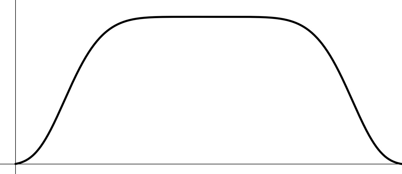
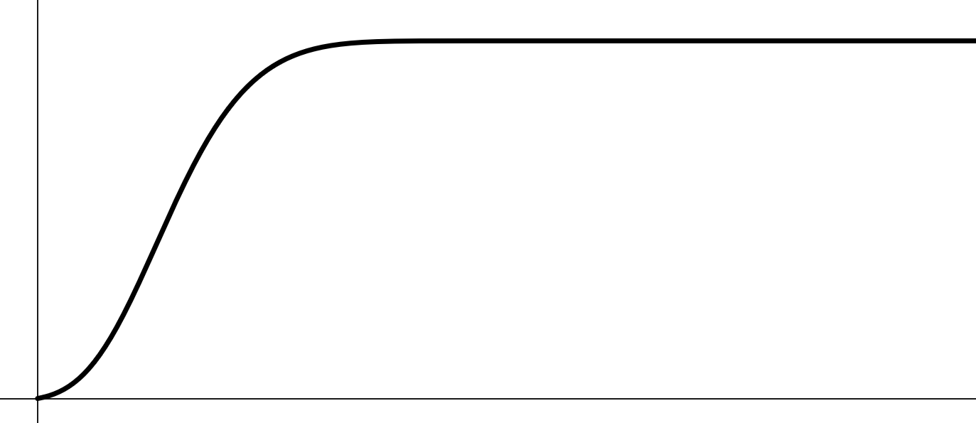
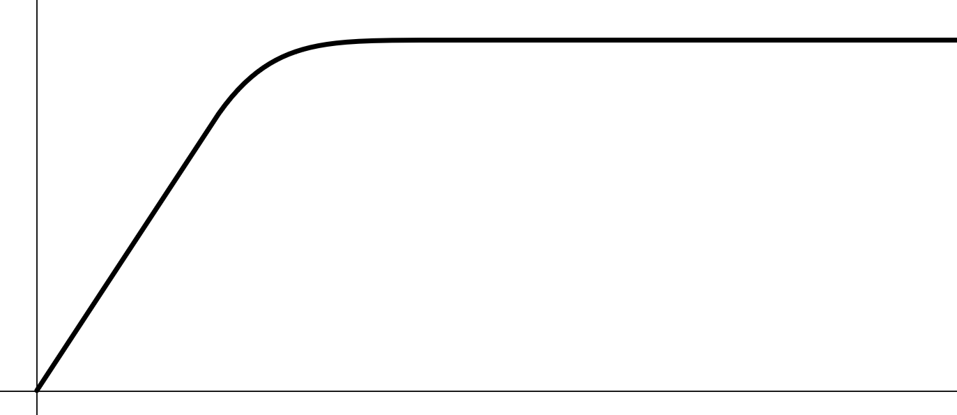
In Figure 6 we show an example of this construction process for a particular $I(x)$ (Fig. 6a), with equivalent nondecreasing oracle functions $J_{1}(x)$ (Fig. 6b), and the full simplification of the proposition, Fig. 6c. We next show that any $G|I$ with a nonzero cost of zero information can be shifted to an equivalent game for which $I(0)=0$.

For $G|I$, let $I(0)=c>0$, and note that $c\leq 1$. Define the following

$$N=M_{I(0)}=(1-c)M+cR,\qquad\qquad J(x)=\frac{I(x)-c}{1-c}$$

First note that the maximal matrix $R$ is the same for $M$ and $N$, since the highest payoff to A in each column of $M_{I}$ is the same for all values of $I$. Also, $J(x)$ will be continuous, nondecreasing, and concave down if $I(x)$ is, and $J(0)=0$ since $I(0)=c$. Additionally, $J(x)$ will reach 1 at the same $x$ value that $I(x)$ does.

Then for any $x$, $N_{J(x)}=(1-J(x))N+J(x)R$
= $(1-\frac{I(x)-c}{1-c})((1-c)M+cR)+\frac{I(x)-c}{1-c}R$
= $(1-c)M-(I(x)-c)M+cR-cR\frac{I(x)-c}{1-c}+R\frac{I(x)-c}{1-c}$
= $(1-I(x))M+cR+(I(x)-c)R$
= $(1-I(x))M+I(x)R$
Which is $M_{I(x)}$ by definition. $\blacksquare$
Therefore it is sufficient to only consider oracle functions with $I(0)=0$. For the remainder of this paper, we assume without loss of generality that all oracle functions are continuous, nondecreasing, (weakly) concave down, and satisfy $I(0)=0$.

We first show the conditions under which an equilibrium exists for an Oracle Game, followed by the conditions for a rational strategy to become dominated when enough information has been purchased. We then find the conditions and properties of the transitions occuring in these games as strategies become dominated or undominated.

Proof: Condition 1 holds if and only if player A or B have no incentive to change $s_{a}$ or $s_{b}$ respectively. If we express player A’s payoff as $E_{a}(s_{a},s_{b},I(x))-x$, then it suffices to find a global maximum of this function on its domain. Taking the derivative with respect to $x$ and setting equal to zero yields

$$\frac{\partial E_{a}}{\partial I}\frac{dI}{dx}-1=0$$

assuming that $s_{b}$ is constant. Since $V=\partial E_{a}/\partial I$ by definition, this is equivalent to condition 2, and shows that it yields a local maximum. $V\geq 0$ and $I$ is (weakly) concave down imply that $E_{a}(s_{a},s_{b},I(x))-x$ is also concave down with respect to $x$, so any local maximum must be a global maximum. $\blacksquare$

Proof: Although $I(x)$ will not be differentiable at the endpoints, (i.e. at $0$ and $x_{1}$ since player A cannot choose values of $x<0$ and gains no benefit beyond $I(x)=1$), we only need to look at the one sided limit in these cases. If $\lim_{x\rightarrow 0^{+}}I^{\prime}(x)\leq\frac{1}{V(s_{b})}$, then player A will gain less benefit from increasing the oracle payment than the increase in cost, and has no incentive to do so. Similarly, if $\lim_{x\rightarrow x_{1}^{-}}I^{\prime}(x)\geq\frac{1}{V(s_{b})}$, then player A will lose more benefit from decreasing the oracle payment than the reduction in cost, (and can gain no more benefit from increasing the cost, since $I$ is capped at 1), so has no incentive to change it. $\blacksquare$

We also note that, even if $I^{\prime}(x)$ has discontinuities, condition 2 of Theorem 1 can be modified to say that $c$ must equal the supremum over all points with $V(s_{b})\cdot I^{\prime}(x)\leq 1$.

For the remainder of the paper, we assume $M$ is a payoff matrix such that $M_{I(x)}$ has a unique Nash equilibrium for each $x$, except possibly at nodes. Then we can define $s_{a}(x)$ and $s_{b}(x)$ as the strategies $s_{a}$ and $s_{b}$ in the unique equilibrium of $M_{I(x)}$ for all $x$ except at nodes. If $x$ is a node and all equilibria at that node have the same $s_{a}$ or $s_{b}$, then $s_{a}(x)$ or $s_{b}(x)$ are defined as the appropriate strategy, while if $s_{a}$ or $s_{b}$ vary across equilibria, then the corresponding function is undefined at that node (in most games we consider, $s_{a}(x)$ will be defined at nodes and $s_{b}(x)$ will not).

We also add the assumption that $I$ is strictly increasing and strictly concave down.

Proof: First consider the case when $s$ becomes dominated by some pure strategy $p$. Let $r_{j}$ be the payoffs to B for strategy $j$ in the matrix $R$ (A’s best strategies when the oracle responds). Let $b_{i,j}$ be the entry in $M$ in the $i$th row and $j$th column for B’s payoff, then the entry in the $i$th row and $j$th column of $M_{I(x)}$ will be

$$c_{i,j,x}=(1-I(x))b_{i,j}+I(x)r_{j}.$$

Define $m_{i,j}=r_{j}-b_{i,j}$, then $c_{i,j,x}=b_{i,j}+I(x)m_{i,j}$. That is, the entries in the matrix will scale linearly with $I$, going from $b_{i,j}$ when $I=0$ and reaching $r_{j}$ when $I=1$. Thus if strategy $s$ is not dominated by $p$ when $x=0$ (and $I(0)=0$), this means there must be a row $k$ such that $b_{k,j}\geq b_{k,p}$. But if it is then dominated by $p$ for some nonzero payment $w$, this means that $b_{k,s}+m_{k,s}I(w)\leq b_{k,p}+m_{k,p}I(w)$. Together these imply that $m_{k,p}>m_{k,s}$ and thus $r_{p}>r_{s}$.

Then for any row $i$, $s$ dominated by $p$ at $w$ implies $b_{i,s}+m_{i,s}I(w)\leq b_{i,p}+m_{i,p}I(w)$.

Case 1: $b_{i,s}>b_{i,p}$. Using the same argument as above, we have $m_{k,p}>m_{k,s}$. Then each of $b_{i,s}+m_{i,s}I(w)$ and $b_{i,p}+m_{i,p}\cdot I(w)$ can be viewed as linear function dependent on $I$, with slope $m$. Then if line $p$ has a greater slope and is above line $s$ at $I(w)$, then for any $x>w$, it will also be greater at $I(x)$ since $I$ is an increasing function.

Case 2: $b_{i,s}\leq b_{i,p}$ Going back to $c_{i,j,x}=(1-I(x))b_{i,j}+I(x)r_{j}$, that is, for every $x$, the elements $c_{i,j,x}$ are weighted averages of $b_{i,j}$ and $r_{j}$. Then since $b_{i,s}\leq b_{i,p}$ and $r_{s}<r_{0}$, then

$$(1-I(x))b_{i,s}+I(x)r_{s}<(1-I(x))b_{i,p}+I(x)r_{p}$$

for all values of $x$.

For any mixed strategy $p$, we can consider a hypothetical pure strategy whose payoffs are the weighted averages of the payoffs of its components (proportional to the probability that they are played). If we let $r_{p}$ be the weighted average of the $r_{j}$ weighted by the frequencies of strategy $j$ in $p$ (instead of simply the best payoff to A in the hypothetical strategy), then the same analysis as above shows that if strategy $s$ becomes dominated by $p$ at some $w$, it will stay dominated by $p$ for all $x>w$. $\blacksquare$

Note that if a strategy starts out dominated at $x=0$, Proposition 4 does not apply. However, if such a strategy becomes undominated at some $x>0$, and then be redominated by another strategy at a greater $x$, Proposition 4 would apply, and that strategy would remain dominated. Thus each strategy corresponds to at most two nodes, and if $G|I$ has finitely many strategies implies, it has finitely many nodes.

Proof: Let M be the payoff matrix. Recall that the cross section matrix $M_{I(x)}$ has payoffs to B, $(1-I)b_{i,j}+Ir_{j}$ where $b_{i,j}$ are the payoffs to B in M, and $r_{j}$ are the payoffs to B corresponding A’s best response in column j. Suppose $s_{a}(x)=(A_{1},A_{2},...A_{m})$ is a mixed strategy of Player A. Then for each $j$, player B’s expected value when playing strategy $j$ is

$$E_{j}=\sum_{i=1}^{n}A_{i}[(1-I)b_{i,j}+Ir_{j}]$$

If we fix a particular interval between two nodes, then the set of B’s pure strategies which are undominated is constant on that interval. Let $n$ be the number of undominated pure strategies for B in that interval. Note that the condition that $M_{I(x)}$ has unique equilibria between nodes implies that A also has $n$ undominated pure strategies. Fix $k$ as the index of one of B’s undominated pure strategies. Then $s_{a}(x)$ can be expressed as the solutions to the simultaneous equations $E_{k}=E_{j}$ for all $j\neq$ 1, and $\sum_{i=1}^{n}A_{i}=1$.

Using the last condition, we obtain

$$A_{m}=1-\sum_{i=1}^{n-1}A_{i}$$

which when substituted into the $E_{j}$ gives

$$E_{j}=\sum_{i=1}^{n-1}A_{i}[(1-I)b_{i,j}+Ir_{j}]+(1-\sum_{i=1}^{n-1}A_{i})[(1-I)b_{n,j}+Ir_{j}]$$

$$=(1-I)b_{n,j}+Ir_{j}+\sum_{i=1}^{n-1}A_{i}(1-I)(b_{i,j}-b_{n,j})$$

Since every instance of $A_{i}$ is multiplied by $1-I$, we define $u_{i}=(1-I)A_{i}$ to get

$$E_{j}=(1-I)b_{n,j}+Ir_{j}+\sum_{i=1}^{n-1}u_{i}(b_{i,j}-b_{n,j})$$

Then we have $n-1$ simultaneous equations with $n-1$ variables $u_{i}$, with the coefficients on all $u_{i}$ in $\mathbb{R}$, and the constant terms have I with degree at most 1. It follows that the solutions must be of the form $u_{i}=a+bI$ for some $a_{i},b_{i}\in\mathbb{R}$. Thus all $A_{i}$ are of the form $\frac{a_{i}+b_{i}I}{(1-I)}$ for some $a_{i},b_{i}$ in $\mathbb{R}$. This suffices to prove the proposition. Additionally, if we have all $b_{i,j}\in\mathbb{Q}$, then $a_{i},b_{i}\in\mathbb{Q}$, and by using the least common denominator of $a_{i}$ and $b_{i}$ we can express this as

$$A_{i}=\frac{a_{i}+b_{i}I}{c_{i}(1-I)}$$

with $a_{i},b_{i},c_{i}\in\mathbb{Z}$ $\blacksquare$

Note that this implies that $s_{a}(x)$ is continuous between nodes. Additionally, the support of $s_{a}(x)$ must be constant between nodes because the support of $s_{b}(x)$ is.

References

- Antonioni et al. (2014) Alberto Antonioni, Maria Paula Cacault, Rafael Lalive, and Marco Tomassini. Know thy neighbor: Costly information can hurt cooperation in dynamic networks. PloS One, 9(10):e110788, 2014. doi: https://doi.org/10.1371/journal.pone.0110788.
- Asahina et al. (2008) Kenta Asahina, Viktoryia Pavlenkovich, and Leslie B Vosshall. The survival advantage of olfaction in a competitive environment. Current Biology, 18(15):1153–1155, 2008. doi: https://doi.org/10.1016/j.cub.2008.06.075.
- Ben-Porath and Kahneman (2003) Elchanan Ben-Porath and Michael Kahneman. Communication in repeated games with costly monitoring. Games and Economic Behavior, 44(2):227–250, 2003. doi: https://doi.org/10.1016/S0899-8256(03)00022-8.
- Chiappori et al. (2002) P.-A. Chiappori, S. Levitt, and T. Groseclose. Testing mixed-strategy equilibria when players are heterogeneous: The case of penalty kicks in soccer. American Economic Review, 92:1138–1151, 2002.
- Eliaz and Schotter (2010) Kfir Eliaz and Andrew Schotter. Paying for confidence: An experimental study of the demand for non-instrumental information. Games and Economic Behavior, 70(2):304–324, 2010. doi: https://doi.org/10.1016/j.geb.2010.01.006.
- Flesch and Perea (2009) János Flesch and Andrés Perea. Repeated games with voluntary information purchase. Games and Economic Behavior, 66(1):126–145, 2009. doi: https://doi.org/10.1016/j.geb.2008.04.015.
- Gabaix et al. (2006) Xavier Gabaix, David Laibson, Guillermo Moloche, and Stephen Weinberg. Costly information acquisition: Experimental analysis of a boundedly rational model. American Economic Review, 96(4):1043–1068, 2006. doi: https://doi.org/10.1257/aer.96.4.1043.
- González-Dıaz et al. (2010) Julio González-Dıaz, Ignacio Garcıa-Jurado, and M. Gloria Fiestras-Janeiro. An introductory course on mathematical game theory. American Mathematical Society, 2010.
- Halpern and Pass (2018) Joseph Y. Halpern and Rafael Pass. Game theory with translucent players. International Journal of Game Theory, 47(3):949–976, 2018. doi: https://doi.org/10.1007/s00182-018-0626-x.
- Harsanyi (1967) John C. Harsanyi. Games with incomplete information played by “Bayesian” players, i–iii: Part i. the basic model. Management Science, 14(3):159–182, 1967. doi: https://doi.org/10.1287/mnsc.14.3.159.
- Hellwig and Veldkamp (2009) Christian Hellwig and Laura Veldkamp. Knowing what others know: Coordination motives in information acquisition. The Review of Economic Studies, 76(1):223–251, 2009. doi: https://doi.org/10.1111/j.1467-937X.2008.00515.x.
- Hu et al. (2018) Youxin Hu, John Kagel, Huanxing Yang, and Lan Zhang. The effects of pre-play communication in a coordination game with incomplete information. SSRN, 2018. doi: http://dx.doi.org/10.2139/ssrn.3156442.
- Martinelli (2007) César Martinelli. Rational ignorance and voting behavior. International Journal of Game Theory, 35(3):315–335, 2007.
- McDonald (1996) John McDonald. Strategy in poker, business and war. WW Norton and Company, 1996.
- Miklós-Thal and Schumacher (2013) Jeanine Miklós-Thal and Heiner Schumacher. The value of recommendations. Games and Economic Behavior, 79:132–147, 2013. doi: https://doi.org/10.1016/j.geb.2013.01.005.
- Morris and Shin (2002) Stephen Morris and Hyun Song Shin. Social value of public information. American Economic Review, 92(5):1521–1534, 2002. doi: https://doi.org/10.1257/000282802762024610.
- Myatt and Wallace (2012) David P Myatt and Chris Wallace. Endogenous information acquisition in coordination games. The Review of Economic Studies, 79(1):340–374, 2012. doi: https://doi.org/10.1093/restud/rdr018.
- Myatt and Wallace (2015) David P Myatt and Chris Wallace. Cournot competition and the social value of information. Journal of Economic Theory, 158:466–506, 2015. doi: https://doi.org/10.1016/j.jet.2014.07.011.
- Reny and Robson (2004) Philip J. Reny and Arthur J. Robson. Reinterpreting mixed strategy equilibria: a unification of the classical and Bayesian views. Games and Economic Behavior, 48:355–384, 2004. doi: https://doi:10.1016/j.geb.2003.09.009.
- Rigos (2018) Alexandros Rigos. Flexible information acquisition in large coordination games. Preprint at https://swopec.hhs.se/lunewp/abs/lunewp2018_030.htm, 2018.
- Ruiz-Hernández et al. (2017) Diego Ruiz-Hernández, Javier Elizalde, and David Delgado-Gómez. Cournot–Stackelberg games in competitive delocation. Annals of Operations Research, 256(1):149–170, 2017. doi: https://doi.org/10.1007/s10479-016-2288-z.
- Sakai (1986) Yasuhiro Sakai. Cournot and Bertrand equilibria under imperfect information. Journal of Economics, 46(3):213–232, 1986. doi: https://doi.org/10.1007/BF01229301.
- Solan and Yariv (2004) Eilon Solan and Leeat Yariv. Games with espionage. Games and Economic Behavior, 47(1):172–199, 2004. doi: https://doi.org/10.1016/S0899-8256(03)00177-5.
- Szkup and Trevino (2015) Michal Szkup and Isabel Trevino. Information acquisition in global games of regime change. Journal of Economic Theory, 160:387–428, 2015. doi: https://doi.org/10.1016/j.jet.2015.10.005.
- Yang (2015) Ming Yang. Coordination with flexible information acquisition. Journal of Economic Theory, 158:721–738, 2015.