Span Recovery for Deep Neural Networks with Applications to Input Obfuscation

Consider the general framework in which we are given an unknown function $f:\mathbb{R}^{n}\to\mathbb{R}$, and we want to learn properties about this function given only access to the value $f(x)$ for different inputs $x$. There are many contexts where this framework is applicable, such as blackbox optimization in which we are learning to optimize $f(x)$ [DKC13], PAC learning in which we are learning to approximate $f(x)$ [Den98], adversarial attacks in which we are trying to find adversarial inputs to $f(x)$ [SZS+13], or structure recovery in which we are learning the structure of $f(x)$. For example in the case when $f(x)$ is a neural network, one might want to recover the underlying weights or architecture [ABGM14, ZPSR17]. In this work, we consider the setting when $f(x)=M(x)$ is a neural network that admits a latent low-dimensional structure, namely $M(x)=\sigma(\mathbf{A}x)$ where $\mathbf{A}\in\mathbb{R}^{k\times n}$ is a rank $k$ matrix for some $k<n$, and $\sigma:\mathbb{R}^{k}\to\mathbb{R}$ is some neural network. In this setting, we focus primarily on the goal of recovering the row-span of the weight matrix $\mathbf{A}$. We remark that all our results generalize in a straightforward manner to the case when $\mathbf{A}$ is rank $r<k$.

Span recovery of general functions $f(x)=g(\mathbf{A}x)$, where $g$ is arbitrary, has been studied in some contexts, and is used to gain important information about the underlying function $f$. By learning Span$(\mathbf{A})$, we in essence are capturing the relevant subspace of the input to $f$; namely, $f$ behaves identically on $x$ as it does on the projection of $x$ onto the row-span of $\mathbf{A}$. In statistics, this is known as effective dimension reduction or the multi-index model [Li91, XTLZ02]. Another important motivation for span recovery is for designing adversarial attacks. Given the span of $\mathbf{A}$, we compute the kernel of $\mathbf{A}$, which can be used to fool the function into behaving incorrectly on inputs which are perturbed by vectors in the kernel. Specifically, if $x$ is a legitimate input correctly classified by $f$ and $y$ is a large random vector in the kernel of $\mathbf{A}$, then $x+y$ will be indistinguishable from noise but we will have $f(x)=f(x+y)$.

Several works have considered the problem from an approximation-theoretic standpoint, where the goal is to output a hypothesis function $\widetilde{f}$ which approximates $f$ well on a bounded domain. For instance, in the case that $\mathbf{A}\in\mathbb{R}^{n}$ is a rank 1 matrix and $g(\mathbf{A}x)$ is a smooth function with bounded derivatives, [CDD+12] gives an adaptive algorithm to approximate $f$. Their results also give an approximation $\widetilde{\mathbf{A}}$ to $\mathbf{A}$, under the assumption that $\mathbf{A}$ is a stochastic vector ($\mathbf{A}_{i}\geq 0$ for each $i$ and $\sum_{i}\mathbf{A}_{i}=1$). Extending this result to more general rank $k$ matrices $\mathbf{A}\in\mathbb{R}^{k\times n}$, [TC14] and [FSV12] give algorithms with polynomial sample complexity to find approximations $\widetilde{f}$ to twice differentiable functions $f$. However, their results do not provide any guarantee that the original matrix $\mathbf{A}$ itself or a good approximation to its span will be recovered. Specifically, the matrix $\widetilde{\mathbf{A}}$ used in the hypothesis function $\widetilde{f}(x)=\widetilde{g}(\widetilde{\mathbf{A}}x)$ of [TC14] only has moderate correlation with the true row span of $\mathbf{A}$, and always admits some constant factor error (which can translate into very large error in any subspace approximation).

Furthermore, all aforementioned works require the strong assumption that the matrix of gradients is well-conditioned (and full rank) in order to obtain good approximations $\widetilde{f}$. In contrast, when $f(x)$ is a non-differentiable ReLU deep network with only mild assumptions on the weight matrices, we prove that the gradient matrix has rank at least $k/2$, which significantly strengthens span recovery guarantees since we do not make any assumptions on the gradient matrix. Finally, [HW13] gives an adaptive approximate span recovery algorithm with $\text{poly}(n)$ samples under the assumption that the function $g$ satisfies a norm-preserving condition, which is restrictive and need not (and does not) hold for the deep neural networks we consider here.

On the empirical side, the experimental results of [TC14] for function approximation were only carried out for simple one-layer functions, such as the logistic function in one dimension (where $\mathbf{A}$ has rank $k=1)$, and on linear functions $g^{T}(\mathbf{A}x+b)$, where $g\in\mathbb{R}^{k}$ has i.i.d. Gaussian entries. Moreover, their experiments only attempted to recover approximations $\widetilde{\mathbf{A}}$ to $\mathbf{A}$ when $\mathbf{A}$ was orthonormal. In addition, [FSV12] experimentally considers the approximation problem for $f$ when $f(\mathbf{A}x)$ is a third degree polynomial of the input. This leaves an experimental gap in understanding the performance of span recovery algorithms on non-smooth, multi-layer deep neural networks.

When $f(x)$ is a neural network, there have been many results that allow for weight or architecture recovery under additional assumptions; however nearly all such results are for shallow networks. [ABGM14] shows that layer-wise learning can recover the architecture of random sparse neural networks. [JSA15] applies tensor methods to recover the weights of a two-layer neural network with certain types of smooth activations and vector-valued output, whereas [GKLW19, BJW19] obtain weight recovery for ReLU activations. [ZPSR17] shows that SGD can learn the weights of two-layer neural networks with some specific activations. There is also a line of work for improperly two-layer networks, where the algorithm outputs an arbitrary hypothesis function which behaves similarly to the network under a fixed distribution [GKKT17, GK19].

Learning properties of the network can also lead to so-called model extraction attacks or enhance classical adversarial attacks on neural networks [JCB+19]. Adversarial attacks are often differentiated into two settings, the whitebox setting where the trained network weights are known or the blackbox setting where the network weights are unknown but attacks can still be achieved on external information, such as knowledge of the dataset, training algorithm, network architecture, or network predictions. Whitebox attacks are well-studied and usually use explicit gradients or optimization procedures to compute adversarial inputs for various tasks such as classification and reinforcement learning [SZS+13, HPG+17, GSS14]. However, blackbox attacks are more realistic and it is clear that model recovery can enhance these attacks. The work of [PMG+17] attacks practical neural networks upon observations of predictions of adaptively chosen inputs, trains a substitute neural network on the observed data, and applies a whitebox attack on the substitute. This setting, nicknamed the practical blackbox setting [CZS+17], is what we work in, as we only observe adaptively chosen predictions without knowledge of the network architecture, dataset, or algorithms. We note that perhaps surprisingly, some of our algorithms are in fact entirely non-adaptive.

In this section, we demonstrate that partial span recovery is possible for deep ReLU networks. Specifically, we consider neural networks $M(x):\mathbb{R}^{n}\to\mathbb{R}$ of the form

where $\phi(x)_{i}=\max\{x_{i},0\}$ is the RELU (applied coordinate-wise to each of its inputs), and $\mathbf{W}_{i}\in\mathbb{R}^{k_{i}\times k_{i+1}}$, and $w\in\mathbb{R}^{k_{d}}$, and $\mathbf{A}$ has rank $k$. We note that $k_{i}$ can be much smaller than $k$. In order to obtain partial span recovery, we make the following assumptions parameterized by a value $\gamma>0$ (our algorithms will by polynomial in $1/\gamma$):

• •

  Assumption 1: For every sign pattern $S\in\{0,1\}^{k}$, we have $\mathbf{Pr}_{g\sim\mathcal{N}(0,I_{n})}\left[\text{sign}(\phi(\mathbf{A}g))=S\right]\geq\gamma/2^{k}$.

• •

  Assumption 2: For any $S_{1},\dots,S_{d}\neq\emptyset$ where $S_{i}\subseteq[k_{i}]$, we have $w^{T}\left(\prod_{i=1}^{d}(\mathbf{W}_{i})_{S_{i}}\right)\in\mathbb{R}^{k}$ is entry-wise non-zero. Here $(\mathbf{W}_{i})_{S_{i}}$ is the matrix with the rows $j\notin S_{i}$ set equal to $0$. Moreover, we assume

  $$\mathbf{Pr}_{g\sim\mathcal{N}(0,I_{k})}\left[M(g)=0\right]\leq\frac{\gamma}{8}.$$

Our first assumption is an assumption on the orthant probabilities of the distribution $\mathbf{A}g$. Specifically, observe that $\mathbf{A}g\in\mathbb{R}^{k}$ follows a multi-variate Gaussian distribution with covariance matrix $\mathbf{A}\mathbf{A}^{T}$. Assumption $1$ then states that the probability that a random vector $x\sim\mathcal{N}(0,\mathbf{A}\mathbf{A}^{T})$ lies in a certain orthant of $\mathbb{R}^{k}$ is not too far from uniform. We remark that orthant probabilities of multivariate Gaussian distributions are well-studied (see e.g., [MHK03, Bac63, Abr64]), and thus may allow for the application of this assumption to a larger class of matrices. In particular, we show it is satisfied by both random matrices and orthogonal matrices. Our second assumption is a non-degeneracy condition on the weight matrices $\mathbf{W}_{i}$ – namely, that products of $w^{T}$ with non-empty sets of rows of the $\mathbf{W}_{i}$ result in entry-wise non-zero vectors. In addition, Assumption $2$ requires that the network is non-zero with probability that is not arbitrarily small, otherwise we cannot hope to find even a single $x$ with $M(x)\neq 0$.

In the following lemma, we demonstrate that these conditions are satisfied by randomly initialized networks, even when the entries of the $\mathbf{W}_{i}$ are not identically distributed. The proof can be found in Appendix A.

In this section, we consider networks that have a threshold function at the output node, as is done often for classification. Specifically, let $\tau:\mathbb{R}\to\{0,1\}$ be the threshold function: $\tau(x)=1$ if $x\geq 1$, and $\tau(x)=0$ otherwise. Again, we let $\mathbf{A}\in\mathbb{R}^{k\times n}$ where $k<n$, be the innermost weight matrix. The networks $M:\mathbb{R}^{n}\to\mathbb{R}$ we consider are then of the form:

where $\mathbf{W}_{i}\in\mathbb{R}^{k_{i}\times k_{i+1}}$ and each $\phi_{i}$ is a continuous, differentiable activation function applied entrywise to its input. We will demonstrate that even for such functions with a binary threshold placed at the end, giving us minimal information about the network, we can still achieve full span recovery of the weight matrix $\mathbf{A}$, albeit with the cost of an $\epsilon$-approximation to the subspace. Note that the latter fact is inherent, since the gradient of any function that is not linear in some ball around each point cannot be obtained exactly without infinitely small perturbations of the input, which we do not allow in our model.

We can simplify the above notation, and write $\sigma(x)=\mathbf{W}_{1}\phi_{1}(\mathbf{W}_{2}\phi_{2}(\dots\phi_{d}\mathbf{A}x))\dots)$, and thus $M(x)=\tau(\sigma(x))$. Our algorithm will involve building a subspace $V\subset\mathbb{R}^{n}$ which is a good approximation to the span of $\mathbf{A}$. At each step, we attempt to recover a new vector which is very close to a vector in Span$(\mathbf{A})$, but which is nearly orthogonal to the vectors in $V$. Specifically, after building $V$, on an input $x\in\mathbb{R}^{n}$, we will query $M$ for inputs $M((\mathbb{I}_{n}-\mathbf{P}_{V})x)$. Recall that $\mathbf{P}_{V}$ is the projection matrix onto $V$, and $\mathbf{P}_{V^{\bot}}$ is the projection matrix onto the subspace orthogonal to $V$. Thus, it will help here to think of the functions $M,\sigma$ as being functions of $x$ and not $(\mathbb{I}_{n}-\mathbf{P}_{V})x$, and so we define $\sigma_{V}(x)=\sigma(\mathbf{A}(\mathbb{I}_{n}-\mathbf{P}_{V})x)$, and similarly $M_{V}(x)=\tau(\sigma_{V}(x))$. For the results of this section, we make the following assumptions on the activation functions.

1. 1.

   The function $\phi_{i}:\mathbb{R}\to\mathbb{R}$ is continuous and twice differentiable, and $\phi_{i}(0)=0$.

2. 2.

   $\phi_{i}$ and $\phi_{i}^{\prime}$ are $L_{i}$-Lipschitz, meaning:

   $$\sup_{x\in\mathbb{R}}\left|\frac{d}{dx}\phi_{i}(x)\right|\leq L_{i},\;\;\;\sup_{x\in\mathbb{R}}\left|\frac{d^{2}}{d^{2}x}\phi_{i}(x)\right|\leq L_{i}$$

3. 3.

   The network is non-zero with bounded probability: for every subspace $V\subset\mathbb{R}^{n}$ of dimension dim$(V)<k$, we have that $\mathbf{Pr}_{g\sim\mathcal{N}(0,\mathbb{I}_{n})}\left[\sigma_{V}(g)\geq 1\right]\geq\gamma$ for some value $\gamma>0$.

4. 4.

   Gradients are not arbitrarily small near the boundary: for every subspace $V\subset\mathbb{R}^{n}$ of dimension dim$(V)<k$

   $$\mathbf{Pr}_{g\sim\mathcal{N}(0,\mathbb{I}_{n})}\left[\;\left|\nabla_{g}\sigma_{V}(cg)\right|\geq\eta,\forall c>0\text{ such that }\sigma_{V}(cg)=1,\text{ and }\sigma_{V}(g)\geq 1\right]\geq\gamma$$

   for some values $\eta,\gamma>0$, where $\nabla_{g}\sigma_{V}(cg)$ is the directional derivative of $\sigma_{V}$ in the direction $g$.
   

The first two conditions are standard and straightforward, namely $\phi_{i}$ is differentiable, and has bounded first and second derivatives (note that for our purposes, they need only be bounded in a ball of radius $\text{poly}(n)$). Since $M(x)$ is a threshold applied to $\sigma(x)$, the third condition states that it is possible to find inputs $x$ with non-zero network evaluation $M(x)$. Our condition is slightly stronger, in that we would like this to be possible even when $x$ is projected away from any $k^{\prime}<k$ dimensional subspace (note that this ensures that $\mathbf{A}x$ is non-zero, since $\mathbf{A}$ has rank $k$).

The last condition simply states that if we pick a random direction $g$ where the network is non-zero, then the gradients of the network are not arbitrarily small along that direction at the threshold points where $\sigma(c\cdot g)=1$. Observe that if the gradients at such points are vanishingly small, then we cannot hope to recover them. Moreover, since $M$ only changes value at these points, these points are the only points where information about $\sigma$ can be learned. Thus, the gradients at these points are the only gradients which could possibly be learned. We note that the running time of our algorithms will be polynomial in $\log(1/\eta)$, and thus we can even allow the gradient size $\eta$ to be exponentially small.

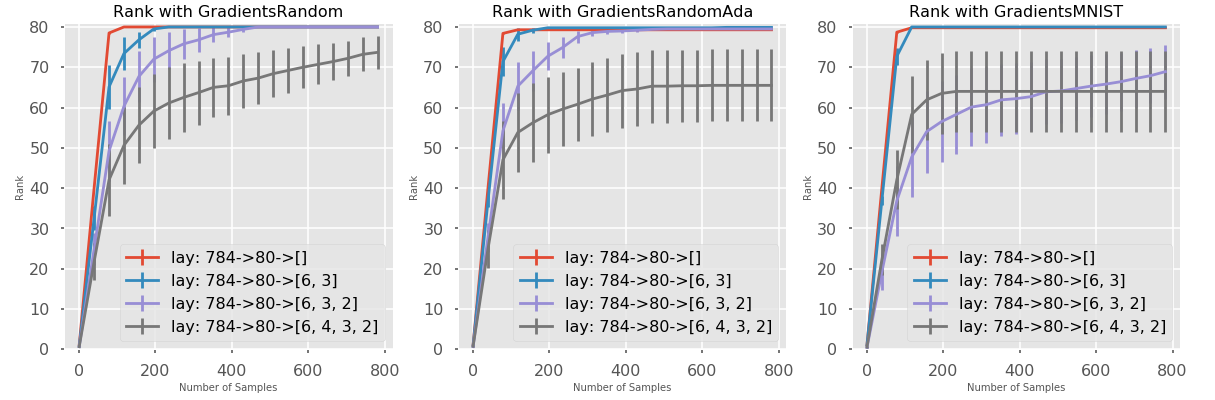
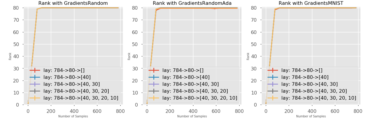
When applying span recovery for a given network, we first calculate the gradients analytically via auto-differentiation at a fixed number of sample points distributed according to a standard Gaussian. Our networks are feedforward, fully-connected with ReLU units; therefore, as mentioned above, using analytic gradients is as precise as using finite differences due to piecewise linearity. Then, we compute the rank of the resulting gradient matrix, where the rank is defined to be the number of singular values that are above 1e-5 of the maximum singular value. In our experiments, we attempt to recover the full span of a 784-by-80 matrix with decreasing layer sizes for varying sample complexity, as specified in the figures. For the MNIST dataset, we use a size 10 vector output and train according to the softmax cross entropy loss, but we only calculate the gradient with respect to the first output node.

Our recovery algorithms are GradientsRandom (Algorithm 1), GradientsRandomAda (Algorithm 2), and GradientsMNIST. GradientsRandom is a direct application of our first span recovery algorithm and calculates gradients via perturbations at random points for a random network. GradientsRandomAda uses our adaptive span recovery algorithm for a random network. Finally, GradientsMNIST is an application of GradientsRandom on a network with weights trained on MNIST data. In general, we note that the experimental outcomes are very similar among all three scenarios.

For networks with very small widths and multiple layers, we see that span recovery deteriorates as depth increases, supporting our theory (see Figure 1). This holds both in the case when the networks are randomly initialized with Gaussian weights or trained on a real dataset (MNIST) and whether we use adaptive or non-adaptive recovery algorithms. However, we note that these small networks have unrealistically small widths (less than 10) and when trained on MNIST, these networks fail to achieve high accuracy, all falling below 80 percent. The small width case is therefore only used to support, with empirical evidence, why our theory cannot possibly guarantee full span recovery under every network architecture.

For more realistic networks with moderate or high widths, however, full span recovery seems easy and implies a real possibility for attack (see Figure 2). Although we tried a variety of widths and depths, the results are robust to reasonable settings of layer sizes and depths. Therefore, we only present experimental results with sub-networks of a network with layer sizes [784, 80, 40, 30, 20, 10]. Note that full span recovery of the first-layer weight matrix with rank 80 is achieved almost immediately in all cases, with less than 100 samples.

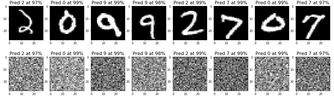
On the real dataset MNIST, we demonstrate the utility of span recovery algorithms as an attack to fool neural networks to misclassify noisy inputs (see Figure 3). We train a ReLU network (to around $95$ percent accuracy) and recover its span by computing the span of the resulting gradient matrix. Then, we recover the null space of the matrix and generate random Gaussian noise projected onto the null space. We see that our attack successfully converts images into noisy versions without changing the output of the network, implying that allowing a full (or even partial) span recovery on a classification network can lead to various adversarial attacks despite not knowing the exact weights of the network.

References

- [ABGM14] Sanjeev Arora, Aditya Bhaskara, Rong Ge, and Tengyu Ma. Provable bounds for learning some deep representations. In International Conference on Machine Learning, pages 584–592, 2014.
- [Abr64] IG Abrahamson. Orthant probabilities for the quadrivariate normal distribution. The Annals of Mathematical Statistics, 35(4):1685–1703, 1964.
- [Bac63] Ralph Hoyt Bacon. Approximations to multivariate normal orthant probabilities. The Annals of Mathematical Statistics, 34(1):191–198, 1963.
- [BJW19] Ainesh Bakshi, Rajesh Jayaram, and David P Woodruff. Learning two layer rectified neural networks in polynomial time. In Proceedings of the Thirty-Second Conference on Learning Theory (COLT), volume 99 of Proceedings of Machine Learning Research, pages 195–268, Phoenix, USA, 25–28 Jun 2019. PMLR.
- [CDD+12] Albert Cohen, Ingrid Daubechies, Ronald DeVore, Gerard Kerkyacharian, and Dominique Picard. Capturing ridge functions in high dimensions from point queries. Constructive Approximation, 35(2):225–243, 2012.
- [Coo18] Nicholas Cook. Lower bounds for the smallest singular value of structured random matrices. The Annals of Probability, 46(6):3442–3500, 2018.
- [CZS+17] Pin-Yu Chen, Huan Zhang, Yash Sharma, Jinfeng Yi, and Cho-Jui Hsieh. Zoo: Zeroth order optimization based black-box attacks to deep neural networks without training substitute models. In Proceedings of the 10th ACM Workshop on Artificial Intelligence and Security, pages 15–26. ACM, 2017.
- [Den98] François Denis. Pac learning from positive statistical queries. In International Conference on Algorithmic Learning Theory, pages 112–126. Springer, 1998.
- [DKC13] Josip Djolonga, Andreas Krause, and Volkan Cevher. High-dimensional gaussian process bandits. In Advances in Neural Information Processing Systems, pages 1025–1033, 2013.
- [FSV12] Massimo Fornasier, Karin Schnass, and Jan Vybiral. Learning functions of few arbitrary linear parameters in high dimensions. Foundations of Computational Mathematics, 12(2):229–262, 2012.
- [GK19] Surbhi Goel and Adam R. Klivans. Learning neural networks with two nonlinear layers in polynomial time. In Proceedings of the Thirty-Second Conference on Learning Theory (COLT), volume 99 of Proceedings of Machine Learning Research, pages 1470–1499, Phoenix, USA, 25–28 Jun 2019. PMLR.
- [GKKT17] Surbhi Goel, Varun Kanade, Adam Klivans, and Justin Thaler. Reliably learning the relu in polynomial time. In Conference on Learning Theory, pages 1004–1042, 2017.
- [GKLW19] Rong Ge, Rohith Kuditipudi, Zhize Li, and Xiang Wang. Learning two-layer neural networks with symmetric inputs. In International Conference on Learning Representations, 2019.
- [GSS14] Ian J Goodfellow, Jonathon Shlens, and Christian Szegedy. Explaining and harnessing adversarial examples. arXiv preprint arXiv:1412.6572, 2014.
- [HHMS10] H Tracy Hall, Leslie Hogben, Ryan Martin, and Bryan Shader. Expected values of parameters associated with the minimum rank of a graph. Linear Algebra and its Applications, 433(1):101–117, 2010.
- [HPG+17] Sandy Huang, Nicolas Papernot, Ian Goodfellow, Yan Duan, and Pieter Abbeel. Adversarial attacks on neural network policies. arXiv preprint arXiv:1702.02284, 2017.
- [HW13] Moritz Hardt and David P Woodruff. How robust are linear sketches to adaptive inputs? In Proceedings of the forty-fifth annual ACM symposium on Theory of computing, pages 121–130. ACM, 2013.
- [JCB+19] Matthew Jagielski, Nicholas Carlini, David Berthelot, Alex Kurakin, and Nicolas Papernot. High-fidelity extraction of neural network models. arXiv preprint arXiv:1909.01838, 2019.
- [JSA15] Majid Janzamin, Hanie Sedghi, and Anima Anandkumar. Beating the perils of non-convexity: Guaranteed training of neural networks using tensor methods. arXiv preprint arXiv:1506.08473, 2015.
- [Li91] Ker-Chau Li. Sliced inverse regression for dimension reduction. Journal of the American Statistical Association, 86(414):316–327, 1991.
- [LM00] B. Laurent and P. Massart. Adaptive estimation of a quadratic functional by model selection. Ann. Statist., 28(5):1302–1338, 10 2000.
- [MHK03] Tetsuhisa Miwa, AJ Hayter, and Satoshi Kuriki. The evaluation of general non-centred orthant probabilities. Journal of the Royal Statistical Society: Series B (Statistical Methodology), 65(1):223–234, 2003.
- [PMG+17] Nicolas Papernot, Patrick McDaniel, Ian Goodfellow, Somesh Jha, Z Berkay Celik, and Ananthram Swami. Practical black-box attacks against machine learning. In Proceedings of the 2017 ACM on Asia conference on computer and communications security, pages 506–519. ACM, 2017.
- [SZS+13] Christian Szegedy, Wojciech Zaremba, Ilya Sutskever, Joan Bruna, Dumitru Erhan, Ian Goodfellow, and Rob Fergus. Intriguing properties of neural networks. arXiv preprint arXiv:1312.6199, 2013.
- [TC14] Hemant Tyagi and Volkan Cevher. Learning non-parametric basis independent models from point queries via low-rank methods. Applied and Computational Harmonic Analysis, 37(3):389–412, 2014.
- [Ver10] Roman Vershynin. Introduction to the non-asymptotic analysis of random matrices. arXiv preprint arXiv:1011.3027, 2010.
- [XTLZ02] Yingcun Xia, Howell Tong, Wai Keungxs Li, and Li-Xing Zhu. An adaptive estimation of dimension reduction space. Journal of the Royal Statistical Society: Series B (Statistical Methodology), 64(3):363–410, 2002.
- [ZPSR17] Qiuyi Zhang, Rina Panigrahy, Sushant Sachdeva, and Ali Rahimi. Electron-proton dynamics in deep learning. arXiv preprint arXiv:1702.00458, pages 1–31, 2017.
Appendix A Missing Proofs from Section 3
We first restate the results which have had their proofs omitted, and include their proofs subsequently.
Lemma 3.1
If has orthogonal rows, or if and has entries that are drawn i.i.d. from some sub-Gaussian distribution with expectation , unit variance, and constant sub-gaussian norm then with probability at least , satisfies Assumption 1 with .
Moreover, if the weight matrices with have entries that are drawn independently (and possibly non-identically) from continuous symmetric distributions, and if for each , then Assumption holds with probability .
Proof.
By Theorem 5.58 of [Ver10], if the entries are drawn i.i.d. from some sub-Gaussian isotropic distribution over such that almost surely, then with probability at least , for some constants depending only on . Since the entries are i.i.d. with variance , it follows that the rows of are isotropic. Moreover, we can always condition on the rows having norm exactly , and pulling out a positive diagonal scaling through the first Relu of , and absorbing this scaling into . It follows that the conditions of the theorem hold, and we have with probability at least for a suitably large re scaling of the constant . Setting , it follows that , which holds immediately if has orthogonal rows.
Now observe that is distributed as a multi-variate Gaussian with co-variance , and is therefore given by the probability density function (pdf)
Let be the pdf of an identity covariance Gaussian . We lower bound for with . In this case, we have