First order least-squares formulations for eigenvalue problems

Fleurianne Bertrand Address: Humboldt-Universität zu Berlin, Germany and King Abdullah University of Science and Technology, Saudi Arabia Current address: Email address: and Daniele Boffi Address: King Abdullah University of Science and Technology, Saudi Arabia, and University of Pavia, Italy Current address: Email address:

Abstract.

In this paper we discuss spectral properties of operators associated with the least-squares finite element approximation of elliptic partial differential equations. The convergence of the discrete eigenvalues and eigenfunctions towards the corresponding continuous eigenmodes is studied and analyzed with the help of appropriate $L^{2}$ error estimates. A priori and a posteriori estimates are proved.

1. Introduction

Least-squares finite element formulations have been successfully used for the approximation of several problems described in terms of partial differential equations.

In particular, we are considering formulations that approximate simultaneously scalar (potential) and vector (flux) variables in the spirit of first-order system least squares [4]. While least-squares schemes posses an inherent error control and are particularly suited for problems involving coupling conditions, other approaches involving mixed or hybrid schemes [6] enjoy good conservation properties. The closedness property from [10] show how sometimes results from one approach can be transferred to the other one.

Only few papers deal with eigenvalue problems associated with least-squares formulations. In [8] the authors apply their theory to a second order least-squares formulation of a Dirichlet eigenvalue problem. In [9] a first order least-squares formulation is introduced for the approximation of the eigenvalues of Maxwell’s equations.

In this paper we aim at investigating the least-squares finite element approximation of the eigensolutions of operators associated with second order elliptic equations. Even if the proposed method may be not competitive with other solution techniques, the presented analysis sheds some light on fundamental properties of least-squares formulations, in particular in connection with the simulation of evolution problems.

We start with presenting several least-squares formulations for the approximation of the eigensolutions of the Diriclet Laplace problem. For each formulation we characterize the eigenmodes obtained after finite element discretization and we describe the structure of the underlined algebraic systems.

We then discuss the convergence of the discrete solutions towards the continuous eigenmodes. We use the standard theory of the approximation of compact operators (see [3, 5] and the references therein); it can be easily seen that standard energy estimates (in the graph norm) are not enough to guarantee the uniform convergence of the discrete solution operator sequence to the continuous solution operator. This is a consequence of the known lack of compactness of the solution operator in the energy norm; for this reason, we consider the solution operator in $L^{2}(\Omega)$ and we discuss various $L^{2}(\Omega)$ error estimates. It turns out that in the case of $\operatorname{\mathrm{div}}$ formulations for FOSLS (First order system least-squares) and LL^∗ formulations, if the flux variable is approximated with Raviart–Thomas spaces (or, in general, with other mixed spaces [6]) then the presented approximations are optimally convergent. On the other hand, the corresponding $\operatorname{\mathrm{div}}$ – $\operatorname{\mathbf{curl}}$ formulations suffer, as expected, from serious issues when applied to singular solutions such as those occurring when the computational domain presents reentrant corners; in this case continuous finite elements cannot correctly approximate the flux which is not $\mathbf{H}^{1}(\Omega)$ regular and the corresponding eigenvalues converge to a wrong solution.

A priori and a posteriori error estimates are presented and rigorously proved for the proposed formulations.

Several numerical tests conclude the paper, confirming our results and investigating situations not covered by the theory.

2. The Laplace eigenvalue problem

The problem we are considering is to find $\lambda\in\mathbb{R}$ and $u$ non vanishing such that

\left\{\begin{aligned} &-\Delta u=\lambda u&&\text{in }\Omega\\ &u=0&&\text{on }\partial\Omega\end{aligned}\right.

Our problem can be written in the following standard first order formulation: find $\lambda\in\mathbb{R}$ and $u$ non vanishing such that for some $\boldsymbol{\sigma}$

\left\{\begin{aligned} &\boldsymbol{\sigma}-\operatorname{\nabla}u=0&&\text{in }\Omega\\ &\operatorname{\mathrm{div}}\boldsymbol{\sigma}=-\lambda u&&\text{in }\Omega\\ &u=0&&\text{on }\partial\Omega\end{aligned}\right.

More general symmetric elliptic problems in divergence form could be considered, as well as different homogeneous boundary conditions. Since all our analysis applies with standard modifications to more general situations, we describe our theory in the simplest possible setting.

2.1. FOSLS formulation

The simplest least squares formulation for the source problem is given by the minimization of the following functional [20]:

\mathcal{F}(\boldsymbol{\tau},v)=\|\boldsymbol{\tau}-\operatorname{\nabla}v\|^{2}+\|\operatorname{\mathrm{div}}\boldsymbol{\tau}+f\|^{2}

If the $L^{2}(\Omega)$ norm is considered, this leads to the following variational formulation: find $\boldsymbol{\sigma}\in\mathbf{H}(\operatorname{\mathrm{div}};\Omega)$ and $u\in H^{1}_{0}(\Omega)$ such that

(1)

\left\{\begin{aligned} &(\boldsymbol{\sigma},\boldsymbol{\tau})+(\operatorname{\mathrm{div}}\boldsymbol{\sigma},\operatorname{\mathrm{div}}\boldsymbol{\tau})-(\operatorname{\nabla}u,\boldsymbol{\tau})=-(f,\operatorname{\mathrm{div}}\boldsymbol{\tau})&&\forall\boldsymbol{\tau}\in\mathbf{H}(\operatorname{\mathrm{div}};\Omega)\\ &-(\boldsymbol{\sigma},\operatorname{\nabla}v)+(\operatorname{\nabla}u,\operatorname{\nabla}v)=0&&\forall v\in H^{1}_{0}(\Omega)\end{aligned}\right.

This formulation can be used in a naturally way to consider the following eigenvalue problem: find $\lambda\in\mathbb{C}$ and $u\in H^{1}_{0}(\Omega)$ with $u\neq 0$ such that for some $\boldsymbol{\sigma}\in\mathbf{H}(\operatorname{\mathrm{div}};\Omega)$ it holds

(F1)

\left\{\begin{aligned} &(\boldsymbol{\sigma},\boldsymbol{\tau})+(\operatorname{\mathrm{div}}\boldsymbol{\sigma},\operatorname{\mathrm{div}}\boldsymbol{\tau})-(\operatorname{\nabla}u,\boldsymbol{\tau})=-\lambda(u,\operatorname{\mathrm{div}}\boldsymbol{\tau})&&\forall\boldsymbol{\tau}\in\mathbf{H}(\operatorname{\mathrm{div}};\Omega)\\ &-(\boldsymbol{\sigma},\operatorname{\nabla}v)+(\operatorname{\nabla}u,\operatorname{\nabla}v)=0&&\forall v\in H^{1}_{0}(\Omega)\end{aligned}\right.

Even if the formulation is not symmetric, it can be easily shown that the eigenvalues are real. We state this result in the next proposition since its proof might have interesting consequences for the numerical approximation of our problem.

Proposition 1.

Problem (F1) admits a sequence of positive eigenvalues

0<\lambda_{1}<\lambda_{2}\leq\lambda_{3}\leq\dots

diverging to $+\infty$ . The corresponding eigenspaces span the space $H^{1}_{0}(\Omega)$ .

Proof.

The result follows by the simple observation that the solution operator associated with problem (1) is exactly the same as for the standard Laplace equation. We would like however to show explicitly that the eigenvalues of (F1) are real since this has interesting implications for the finite element discretization.

The (non symmetric) operator form of problem (F1), with natural notation, is given by

(2)

\left(\begin{matrix}\mathsf{A}&\mathsf{B}^{\top}\\ \mathsf{B}&\mathsf{C}\end{matrix}\right)\left(\begin{matrix}\mathsf{x}\\ \mathsf{y}\end{matrix}\right)=\lambda\left(\begin{matrix}\mathsf{0}&\mathsf{D}\\ \mathsf{0}&\mathsf{0}\end{matrix}\right)\left(\begin{matrix}\mathsf{x}\\ \mathsf{y}\end{matrix}\right)

After integration by parts, thanks to the boundary conditions we have $\mathsf{D}=-\mathsf{B}^{\top}$ so that (2) can be reduced to the following equivalent symmetric Schur complement formulation

(3)

\mathsf{A}\mathsf{x}=(\lambda+1)\mathsf{B}^{\top}\mathsf{C}^{-1}\mathsf{B}\mathsf{x},

where we have used the equality $\mathsf{y}=-\mathsf{C}^{-1}\mathsf{B}\mathsf{x}$ .

Another possible way of observing that (2) corresponds to a symmetric problem is to rearrange its terms as follows

\left(\begin{matrix}\mathsf{A}&\mathsf{0}\\ (\lambda+1)\mathsf{B}&(\lambda+1)\mathsf{C}\end{matrix}\right)\left(\begin{matrix}\mathsf{x}\\ \mathsf{y}\end{matrix}\right)=(\lambda+1)\left(\begin{matrix}\mathsf{0}&-\mathsf{B}^{\top}\\ \mathsf{0}&\mathsf{0}\end{matrix}\right)\left(\begin{matrix}\mathsf{x}\\ \mathsf{y}\end{matrix}\right)

obtaining finally

\left(\begin{matrix}\mathsf{A}&\mathsf{0}\\ \mathsf{0}&\mathsf{0}\end{matrix}\right)\left(\begin{matrix}\mathsf{x}\\ \mathsf{y}\end{matrix}\right)=(\lambda+1)\left(\begin{matrix}\mathsf{0}&-\mathsf{B}^{\top}\\ -\mathsf{B}&-\mathsf{C}\end{matrix}\right)\left(\begin{matrix}\mathsf{x}\\ \mathsf{y}\end{matrix}\right)

∎

Remark 1.

One might think that problem (F1) (see in particular formulation (2)) gives a number of infinite eigenvalues; however, in our formulation of problem (F1) the eigenfunctions we are looking for correspond to the component $u$ of the solution only. We will go back to this remark later when the approximation of (F1) is considered.

2.2. The transpose FOSLS formulation

Since our problem is self-adjoint, another possibility is to consider the transpose of (F1): find $\lambda\in\mathbb{R}$ and $\boldsymbol{\sigma}\in\mathbf{H}(\operatorname{\mathrm{div}};\Omega)$ with $\boldsymbol{\sigma}\neq\mathbf{0}$ such that for some $u\in H^{1}_{0}(\Omega)$ it holds

(F1*)

\left\{\begin{aligned} &(\boldsymbol{\sigma},\boldsymbol{\tau})+(\operatorname{\mathrm{div}}\boldsymbol{\sigma},\operatorname{\mathrm{div}}\boldsymbol{\tau})-(\operatorname{\nabla}u,\boldsymbol{\tau})=0&&\forall\boldsymbol{\tau}\in\mathbf{H}(\operatorname{\mathrm{div}};\Omega)\\ &-(\boldsymbol{\sigma},\operatorname{\nabla}v)+(\operatorname{\nabla}u,\operatorname{\nabla}v)=-\lambda(\operatorname{\mathrm{div}}\boldsymbol{\sigma},v)&&\forall v\in H^{1}_{0}(\Omega)\end{aligned}\right.

This leads to the following operator form

(4)

\left(\begin{matrix}\mathsf{A}&\mathsf{B}^{\top}\\ \mathsf{B}&\mathsf{C}\end{matrix}\right)\left(\begin{matrix}\mathsf{x}\\ \mathsf{y}\end{matrix}\right)=\lambda\left(\begin{matrix}\mathsf{0}&\mathsf{0}\\ \mathsf{D}^{\top}&\mathsf{0}\end{matrix}\right)\left(\begin{matrix}\mathsf{x}\\ \mathsf{y}\end{matrix}\right)

and to the corresponding symmetric Schur complement form

(5)

\mathsf{C}\mathsf{y}=(\lambda+1)\mathsf{B}\mathsf{A}^{-1}\mathsf{B}^{\top}\mathsf{y}

Proposition 2.

Problems (3) and (5) (and hence formulations (F1) and (F1*)) are equivalent.

Proof.

The equivalence can be seen, for instance, by solving the matrix problem (2) for $\mathsf{x}$ , thus obtaining $\mathsf{x}=\mathsf{A}^{-1}(\lambda\mathsf{D}\mathsf{y}-\mathsf{B}^{\top}\mathsf{y})$ which gives $\mathsf{C}\mathsf{y}=(\lambda+1)\mathsf{B}\mathsf{A}^{-1}\mathsf{B}^{\top}\mathsf{y}$ , that is (5). ∎

2.3. The LL^∗ formulation

Another popular choice for the approximation of the problem under consideration is the so called LL^∗ formulation [11]. One of the reasons for its introduction is the possibility to deal with less regular right hand sides; moreover, it gives rise to an intrinsically symmetric formulation, which makes it appealing for the application to eigenvalue problems. In the case of the source problem it reads: find $\boldsymbol{\chi}\in\mathbf{H}(\operatorname{\mathrm{div}};\Omega)$ and $p\in H^{1}_{0}(\Omega)$ such that

(6)

\left\{\begin{aligned} &(\boldsymbol{\chi},\boldsymbol{\xi})+(\operatorname{\mathrm{div}}\boldsymbol{\chi},\operatorname{\mathrm{div}}\boldsymbol{\xi})-(\operatorname{\nabla}p,\boldsymbol{\xi})=0&&\forall\boldsymbol{\xi}\in\mathbf{H}(\operatorname{\mathrm{div}};\Omega)\\ &-(\boldsymbol{\chi},\operatorname{\nabla}q)+(\operatorname{\nabla}p,\operatorname{\nabla}q)=(f,q)&&\forall q\in H^{1}_{0}(\Omega)\end{aligned}\right.

It turns out that this formulation is related to our original Laplace problem by the following relation:

(7)			$\displaystyle-\Delta u=f$
			$\displaystyle-\Delta p=f-u$
			$\displaystyle\boldsymbol{\chi}=\operatorname{\nabla}(p-u)$
			$\displaystyle\operatorname{\mathrm{div}}\boldsymbol{\chi}=u$

The eigenvalue problem associated with (6) is: find $\mu\in\mathbb{R}$ and $p\in H^{1}_{0}(\Omega)$ , with $p\neq 0$ , such that for some $\boldsymbol{\chi}\in\mathbf{H}(\operatorname{\mathrm{div}};\Omega)$ it holds

(LL*)

\left\{\begin{aligned} &(\boldsymbol{\chi},\boldsymbol{\xi})+(\operatorname{\mathrm{div}}\boldsymbol{\chi},\operatorname{\mathrm{div}}\boldsymbol{\xi})-(\operatorname{\nabla}p,\boldsymbol{\xi})=0&&\forall\boldsymbol{\xi}\in\mathbf{H}(\operatorname{\mathrm{div}};\Omega)\\ &-(\boldsymbol{\chi},\operatorname{\nabla}q)+(\operatorname{\nabla}p,\operatorname{\nabla}q)=\mu(p,q)&&\forall q\in H^{1}_{0}(\Omega)\end{aligned}\right.

As already anticipated, this problem is symmetric and it can be written in the following form in terms of the underlined operators:

\left(\begin{matrix}\mathsf{A}&\mathsf{B}^{\top}\\ \mathsf{B}&\mathsf{C}\end{matrix}\right)\left(\begin{matrix}\mathsf{x}\\ \mathsf{y}\end{matrix}\right)=\mu\left(\begin{matrix}\mathsf{0}&\mathsf{0}\\ \mathsf{0}&\mathsf{M}\end{matrix}\right)\left(\begin{matrix}\mathsf{x}\\ \mathsf{y}\end{matrix}\right)

By using the links between the LL^∗ formulation and the original problem, as stated in (7), we can see how to relate the eigenvalues of (LL*) to the ones of the problem we are interested in.

Proposition 3.

The eigenvalues $\mu$ of (LL*) are in one-to-one correspondence with the eigenvalues $\lambda$ of the Laplace eigenproblem using the relation

\lambda=\frac{\mu+\sqrt{\mu^{2}+4}}{2}

Moreover, the eigenfunctions $u$ of the Laplace eigenproblem are given by $\operatorname{\mathrm{div}}\boldsymbol{\chi}$ and their gradients $\operatorname{\nabla}u$ are equal to $\operatorname{\nabla}p-\boldsymbol{\chi}$ .

2.4. Enriching the formulations with $\operatorname{\mathbf{curl}}\boldsymbol{\sigma}$

Since $\boldsymbol{\sigma}$ is a gradient, it satisfies $\operatorname{\mathbf{curl}}\boldsymbol{\sigma}=0$ ; a commonly used modification of the FOSLS methods consists in using a least-squares functional that contains the term $\operatorname{\mathbf{curl}}\boldsymbol{\sigma}$ , that is,

\mathcal{F}(\boldsymbol{\tau},v)=\|\boldsymbol{\tau}-\operatorname{\nabla}v\|^{2}+\|\operatorname{\mathbf{curl}}\boldsymbol{\sigma}\|^{2}+\|\operatorname{\mathrm{div}}\boldsymbol{\tau}+f\|^{2}

With natural modifications the two corresponding formulations read: find $\lambda\in\mathbb{R}$ and $u\in H^{1}_{0}(\Omega)$ with $u\neq 0$ such that for some $\boldsymbol{\sigma}\in\mathbf{H}(\operatorname{\mathrm{div}};\Omega)\cap\mathbf{H}(\operatorname{\mathbf{curl}};\Omega)$ it holds

(F1curl)

\left\{\begin{aligned} &(\boldsymbol{\sigma},\boldsymbol{\tau})+(\operatorname{\mathrm{div}}\boldsymbol{\sigma},\operatorname{\mathrm{div}}\boldsymbol{\tau})+(\operatorname{\mathbf{curl}}\boldsymbol{\sigma},\operatorname{\mathbf{curl}}\boldsymbol{\tau})-(\operatorname{\nabla}u,\boldsymbol{\tau})=-\lambda(u,\operatorname{\mathrm{div}}\boldsymbol{\tau})\\ &\hskip 170.71652pt\forall\boldsymbol{\tau}\in\mathbf{H}(\operatorname{\mathrm{div}};\Omega)\cap\mathbf{H}(\operatorname{\mathbf{curl}};\Omega)\\ &-(\boldsymbol{\sigma},\operatorname{\nabla}v)+(\operatorname{\nabla}u,\operatorname{\nabla}v)=0\hskip 51.21504pt\forall v\in H^{1}_{0}(\Omega)\end{aligned}\right.

and find $\lambda\in\mathbb{R}$ and $\boldsymbol{\sigma}\in\mathbf{H}(\operatorname{\mathrm{div}};\Omega)\cap\mathbf{H}(\operatorname{\mathbf{curl}};\Omega)$ with $\boldsymbol{\sigma}\neq\mathbf{0}$ such that for some $u\in H^{1}_{0}(\Omega)$ it holds

(F1*curl)

\left\{\begin{aligned} &(\boldsymbol{\sigma},\boldsymbol{\tau})+(\operatorname{\mathrm{div}}\boldsymbol{\sigma},\operatorname{\mathrm{div}}\boldsymbol{\tau})+(\operatorname{\mathbf{curl}}\boldsymbol{\sigma},\operatorname{\mathbf{curl}}\boldsymbol{\tau})-(\operatorname{\nabla}u,\boldsymbol{\tau})=0\\ &\hskip 196.32384pt\forall\boldsymbol{\tau}\in\mathbf{H}(\operatorname{\mathrm{div}};\Omega)\cap\mathbf{H}(\operatorname{\mathbf{curl}};\Omega)\\ &-(\boldsymbol{\sigma},\operatorname{\nabla}v)+(\operatorname{\nabla}u,\operatorname{\nabla}v)=-\lambda(\operatorname{\mathrm{div}}\boldsymbol{\sigma},v)\hskip 28.45274pt\forall v\in H^{1}_{0}(\Omega)\end{aligned}\right.

which lead to reduced formulations analogous to the previous ones with appropriate modification of the matrix $\mathsf{A}$ .

Remark 2.

Sometimes formulation (F1curl) is presented in the literature with a different choice of functional spaces, that is $\{\boldsymbol{\sigma},\boldsymbol{\tau}\}\in\mathbf{H}^{1}(\Omega)$ instead of $\{\boldsymbol{\sigma},\boldsymbol{\tau}\}\in\mathbf{H}(\operatorname{\mathrm{div}};\Omega)\cap\mathbf{H}(\operatorname{\mathbf{curl}};\Omega)$ . Although for smooth domains the two spaces are the same, this is not the case when singular solutions are presented, that could be in $\mathbf{H}(\operatorname{\mathrm{div}};\Omega)\cap\mathbf{H}(\operatorname{\mathbf{curl}};\Omega)$ but not in $\mathbf{H}^{1}(\Omega)$ .

In a natural way it is possible to consider the LL^∗ formulation associated to the formulation enriched with $\operatorname{\mathbf{curl}}\boldsymbol{\sigma}$ : find $\boldsymbol{\chi}\in\mathbf{H}(\operatorname{\mathrm{div}};\Omega)\cap\mathbf{H}(\operatorname{\mathbf{curl}};\Omega)$ , $p\in H^{1}_{0}(\Omega)$ , and $z\in H^{1}(\Omega)$ , such that

\left\{\begin{aligned} &(\boldsymbol{\chi},\boldsymbol{\xi})+(\operatorname{\mathrm{div}}\boldsymbol{\chi},\operatorname{\mathrm{div}}\boldsymbol{\xi})+(\operatorname{\mathbf{curl}}\boldsymbol{\chi},\operatorname{\mathbf{curl}}\boldsymbol{\xi})\\ &\hskip 85.35826pt-(\operatorname{\nabla}p,\boldsymbol{\xi})+(\operatorname{\mathbf{curl}}z,\boldsymbol{\xi})=0&&\forall\boldsymbol{\xi}\in\mathbf{H}(\operatorname{\mathrm{div}};\Omega)\cap\mathbf{H}(\operatorname{\mathbf{curl}};\Omega)\\ &-(\boldsymbol{\chi},\operatorname{\nabla}q)+(\operatorname{\nabla}p,\operatorname{\nabla}q)-(\operatorname{\mathbf{curl}}z,\operatorname{\nabla}q)=(f,q)&&\forall q\in H^{1}_{0}(\Omega)\\ &(\boldsymbol{\chi},\operatorname{\mathbf{curl}}w)-(\operatorname{\nabla}p,\operatorname{\mathbf{curl}}w)+(\operatorname{\mathbf{curl}}z,\operatorname{\mathbf{curl}}w)=0&&\forall w\in H^{1}(\Omega)\end{aligned}\right.

The corresponding eigenvalue problem is then: find $\lambda\in\mathbb{R}$ and $p\in H^{1}_{0}(\Omega)$ , with $p\neq 0$ , such that for some $\boldsymbol{\chi}\in\mathbf{H}(\operatorname{\mathrm{div}};\Omega)\cap\mathbf{H}(\operatorname{\mathbf{curl}};\Omega)$ and $z\in H^{1}(\Omega)$ it holds

(LL*curl)

\left\{\begin{aligned} &(\boldsymbol{\chi},\boldsymbol{\xi})+(\operatorname{\mathrm{div}}\boldsymbol{\chi},\operatorname{\mathrm{div}}\boldsymbol{\xi})+(\operatorname{\mathbf{curl}}\boldsymbol{\chi},\operatorname{\mathbf{curl}}\boldsymbol{\xi})\\ &\hskip 85.35826pt-(\operatorname{\nabla}p,\boldsymbol{\xi})+(\operatorname{\mathbf{curl}}z,\boldsymbol{\xi})=0&&\forall\boldsymbol{\xi}\in\mathbf{H}(\operatorname{\mathrm{div}};\Omega)\cap\mathbf{H}(\operatorname{\mathbf{curl}};\Omega)\\ &-(\boldsymbol{\xi},\operatorname{\nabla}q)+(\operatorname{\nabla}p,\operatorname{\nabla}q)-(\operatorname{\mathbf{curl}}z,\operatorname{\nabla}q)=\lambda(p,q)&&\forall q\in H^{1}_{0}(\Omega)\\ &(\boldsymbol{\chi},\operatorname{\mathbf{curl}}w)-(\operatorname{\nabla}p,\operatorname{\mathbf{curl}}w)+(\operatorname{\mathbf{curl}}z,\operatorname{\mathbf{curl}}w)=0&&\forall w\in H^{1}(\Omega)\end{aligned}\right.

The operators structure of this problem is now

\left(\begin{matrix}\mathsf{A}&\mathsf{B}^{\top}&\mathsf{C}^{\top}\\ \mathsf{B}&\mathsf{D}&\mathsf{E}^{\top}\\ \mathsf{C}&\mathsf{E}&\mathsf{F}\end{matrix}\right)\left(\begin{matrix}\mathsf{x}\\ \mathsf{y}\\ \mathsf{z}\end{matrix}\right)=\mu\left(\begin{matrix}\mathsf{0}&\mathsf{0}&\mathsf{0}\\ \mathsf{0}&\mathsf{M}&\mathsf{0}\\ \mathsf{0}&\mathsf{0}&\mathsf{0}\end{matrix}\right)\left(\begin{matrix}\mathsf{x}\\ \mathsf{y}\\ \mathsf{z}\end{matrix}\right)

3. Galerkin discretizazion

We now discuss the Galerkin discretization of the problems we have introduced in the previous section.

3.1. Approximation of the FOSLS formulations

Let $\Sigma_{h}\subset\mathbf{H}(\operatorname{\mathrm{div}};\Omega)$ and $U_{h}\subset H^{1}_{0}(\Omega)$ be conforming finite element spaces. The discretization of (F1) reads: find $\lambda_{h}\in\mathbb{R}$ and $u_{h}\in U_{h}$ with $u_{h}\neq 0$ such that for some $\boldsymbol{\sigma}_{h}\in\Sigma_{h}$ it holds

(F1h)

\left\{\begin{aligned} &(\boldsymbol{\sigma}_{h},\boldsymbol{\tau})+(\operatorname{\mathrm{div}}\boldsymbol{\sigma}_{h},\operatorname{\mathrm{div}}\boldsymbol{\tau})-(\operatorname{\nabla}u_{h},\boldsymbol{\tau})=-\lambda_{h}(u_{h},\operatorname{\mathrm{div}}\boldsymbol{\tau})&&\forall\boldsymbol{\tau}\in\Sigma_{h}\\ &-(\boldsymbol{\sigma}_{h},\operatorname{\nabla}v)+(\operatorname{\nabla}u_{h},\operatorname{\nabla}v)=0&&\forall v\in U_{h}\end{aligned}\right.

Analogously, the approximation of (F1*) has the following form: find $\lambda_{h}\in\mathbb{R}$ and $\boldsymbol{\sigma}_{h}\in\Sigma_{h}$ with $\boldsymbol{\sigma}_{h}\neq\mathbf{0}$ such that for some $u_{h}\in U_{h}$ it holds

(F1*h)

\left\{\begin{aligned} &(\boldsymbol{\sigma}_{h},\boldsymbol{\tau})+(\operatorname{\mathrm{div}}\boldsymbol{\sigma}_{h},\operatorname{\mathrm{div}}\boldsymbol{\tau})-(\operatorname{\nabla}u_{h},\boldsymbol{\tau})=0&&\forall\boldsymbol{\tau}\in\Sigma_{h}\\ &-(\boldsymbol{\sigma}_{h},\operatorname{\nabla}v)+(\operatorname{\nabla}u_{h},\operatorname{\nabla}v)=-\lambda_{h}(\operatorname{\mathrm{div}}\boldsymbol{\sigma}_{h},v)&&\forall v\in U_{h}\end{aligned}\right.

After introducing basis functions of $\Sigma_{h}$ and $U_{h}$ , the matrix structure of Problems (F1h) and (F1*h) are the ones already anticipated in (2) and (4) and that will be repeated in the next two propositions, where we characterize their eigensolutions. We will then show that the relevant eigenmodes of the two formulations are identical.

Before giving a characterization of the eigenvalues of our discrete formulation, we discuss in the following remark the solution of (possibly degenerate) generalized eigenvalue problems.

Remark 3.

In general our discrete problems have the form of a generalized eigenvalue problem

(8)

\mathcal{A}x=\lambda\mathcal{B}x

where the matrices $\mathcal{A}$ and/or $\mathcal{B}$ may be singular. The solution of this problem satisfies the following properties.

(1)

If the matrix $\mathcal{B}$ is invertible, then (8) is equivalent to the standard eigenvalue problem $\mathcal{B}^{-1}\mathcal{A}x=\lambda x$ .
(2)

If $\mathcal{K}=\ker\mathcal{A}\cap\ker\mathcal{B}$ is not trivial then the eigenvalue problem is degenerate and vectors in $\mathcal{K}$ do not correspond to any eigenvalue of (8).
(3)

If the matrix $\mathcal{B}$ has a non-trivial kernel $\ker(\mathcal{B})$ which does not contain any nonzero vector of $\ker(\mathcal{A})$ then it is conventionally assumed that (8) has an eigenvalue $\lambda=\infty$ with eigenspace equal to $\ker(\mathcal{B})$ .
(4)

If $\mathcal{B}$ is singular and $\mathcal{A}$ is not (which is the most common situation in our framework) then it may be convenient to switch the roles of the two matrices and to consider the problem

$\mathcal{B}x=\mu\mathcal{A}x$

Then $(\mu,x)$ with $\mu=0$ corresponds to the eigenmode $(\infty,x)$ of (8); the remaining eigenmodes are $(\lambda,x)$ with $\lambda=1/\mu$ .

The next proposition is related to the eigensolutions to (F1h).

Proposition 4.

Let us consider the following matrices associated with Problem (F1h).

•

$\mathsf{A}$ is the matrix associated with the bilinear form $(\boldsymbol{\sigma},\boldsymbol{\tau})+(\operatorname{\mathrm{div}}\boldsymbol{\sigma},\operatorname{\mathrm{div}}\boldsymbol{\tau})$ ,
•

$\mathsf{B}$ is the matrix associated with the bilinear form $-(\boldsymbol{\sigma},\operatorname{\nabla}v)$ ,
•

$\mathsf{C}$ is the matrix associated with the bilinear form $(\operatorname{\nabla}u,\operatorname{\nabla}v)$ .

Then the following generalized problem (see (2))

\left(\begin{matrix}\mathsf{A}&\mathsf{B}^{\top}\\ \mathsf{B}&\mathsf{C}\end{matrix}\right)\left(\begin{matrix}\mathsf{x}\\ \mathsf{y}\end{matrix}\right)=\lambda_{h}\left(\begin{matrix}\mathsf{0}&-\mathsf{B}^{\top}\\ \mathsf{0}&\mathsf{0}\end{matrix}\right)\left(\begin{matrix}\mathsf{x}\\ \mathsf{y}\end{matrix}\right)

has three families of eigenvalues. More precisely:

(1)

$\lambda_{h}=\infty$ with multiplicity equal to $\dim\Sigma_{h}$ ,
(2)

$\lambda_{h}=\infty$ with multiplicity equal to $\dim\ker(B^{\top})$ ,
(3)

a number of positive eigenvalues $\lambda_{h}$ (counted with their multiplicities) equal to $\operatorname{\mathrm{rank}}(B^{\top})$ .

Proof.

The dimension of the eigenproblem is $\dim\Sigma_{h}+\dim U_{h}$ which is clearly equal to the number of eigenvalues in the three families since $\dim U_{h}=\dim\ker(B^{\top})+\operatorname{\mathrm{rank}}(B^{\top})$ .

The eigenvalues of the first and of the second family are associated to eigenvectors in the kernel of the matrix on the right hand side. Those are of the form $(\mathsf{x},\mathsf{y})^{\top}$ with $\mathsf{x}$ corresponding to any element in $\Sigma_{h}$ and $\mathsf{y}$ corresponding to elements of $U_{h}$ in $\ker(B^{\top})$ .

The eigenvalues of the third family are characterized by looking at the Schur complement

\mathsf{A}\mathsf{x}=(\lambda_{h}+1)\mathsf{B}^{\top}\mathsf{C}^{-1}\mathsf{B}\mathsf{x}

∎

The following proposition is related to the eigensolutions to (F1*h).

Proposition 5.

Let $\mathsf{A}$ , $\mathsf{B}$ , and $\mathsf{C}$ be the matrices introduced in Proposition 4. Then the following generalized eigenvalue problem associated with Problem (F1*h)

\left(\begin{matrix}\mathsf{A}&\mathsf{B}^{\top}\\ \mathsf{B}&\mathsf{C}\end{matrix}\right)\left(\begin{matrix}\mathsf{x}\\ \mathsf{y}\end{matrix}\right)=\lambda_{h}\left(\begin{matrix}\mathsf{0}&\mathsf{0}\\ -\mathsf{B}&\mathsf{0}\end{matrix}\right)\left(\begin{matrix}\mathsf{x}\\ \mathsf{y}\end{matrix}\right)

has three families of eigenvalues. More precisely:

(1)

$\lambda_{h}=\infty$ with multiplicity $\dim U_{h}$ ,
(2)

$\lambda_{h}=\infty$ with multiplicity $\dim\ker(B)$ ,
(3)

a number of positive eigenvalues $\lambda_{h}$ (counted with their multiplicities) equal to $\operatorname{\mathrm{rank}}(B)$ .

Proof.

The proof is analogous to the one of Proposition 4 by considering the corresponding Schur complement

\mathsf{C}\mathsf{y}=(\lambda_{h}+1)\mathsf{B}\mathsf{A}^{-1}\mathsf{B}^{\top}\mathsf{y}

∎

Since we started from a self-adjoint problem, it is not surprising that formulations (F1h) and (F1*h) are indeed equivalent. This will be shown in the next proposition.

Proposition 6.

The eigenmodes of the third families in Propositions (4) and (5) are the same.

Proof.

Solving the matrix formulation of (F1h) (see (2) and Proposition 4) for $\mathsf{x}$ gives $\mathsf{x}=-\mathsf{A}^{-1}(\lambda_{h}\mathsf{B}^{\top}\mathsf{y}+\mathsf{B}^{\top}\mathsf{y})$ , yielding

\mathsf{C}\mathsf{y}=(\lambda_{h}+1)\mathsf{B}\mathsf{A}^{-1}\mathsf{B}^{\top}\mathsf{y},

that is, the Schur complement of the matrix formulation of (F1*h) (see the proof of Proposition 5). ∎

We conclude this section with another equivalent matrix formulation of (F1h) and (F1*h).

Starting from

\left(\begin{matrix}\mathsf{A}&\mathsf{B}^{\top}\\ \mathsf{B}&\mathsf{C}\end{matrix}\right)\left(\begin{matrix}\mathsf{x}\\ \mathsf{y}\end{matrix}\right)=\lambda_{h}\left(\begin{matrix}\mathsf{0}&-\mathsf{B}^{\top}\\ \mathsf{0}&\mathsf{0}\end{matrix}\right)\left(\begin{matrix}\mathsf{x}\\ \mathsf{y}\end{matrix}\right)

we get

\left(\begin{matrix}\mathsf{A}&\mathsf{0}\\ \mathsf{B}&\mathsf{C}\end{matrix}\right)\left(\begin{matrix}\mathsf{x}\\ \mathsf{y}\end{matrix}\right)=(\lambda_{h}+1)\left(\begin{matrix}\mathsf{0}&-\mathsf{B}^{\top}\\ \mathsf{0}&\mathsf{0}\end{matrix}\right)\left(\begin{matrix}\mathsf{x}\\ \mathsf{y}\end{matrix}\right)

and

\left(\begin{matrix}\mathsf{A}&\mathsf{0}\\ (\lambda_{h}+1)\mathsf{B}&(\lambda_{h}+1)\mathsf{C}\end{matrix}\right)\left(\begin{matrix}\mathsf{x}\\ \mathsf{y}\end{matrix}\right)=(\lambda_{h}+1)\left(\begin{matrix}\mathsf{0}&-\mathsf{B}^{\top}\\ \mathsf{0}&\mathsf{0}\end{matrix}\right)\left(\begin{matrix}\mathsf{x}\\ \mathsf{y}\end{matrix}\right)

leading finally to

\left(\begin{matrix}\mathsf{A}&\mathsf{0}\\ \mathsf{0}&\mathsf{0}\end{matrix}\right)\left(\begin{matrix}\mathsf{x}\\ \mathsf{y}\end{matrix}\right)=(\lambda_{h}+1)\left(\begin{matrix}\mathsf{0}&-\mathsf{B}^{\top}\\ -\mathsf{B}&-\mathsf{C}\end{matrix}\right)\left(\begin{matrix}\mathsf{x}\\ \mathsf{y}\end{matrix}\right)

Remark 4.

The analysis presented in this section applies without modifications to the formulations enriched with the curl. The only change is the definition of the matrix $\mathsf{A}$ which corresponds to the bilinear form $(\boldsymbol{\sigma},\boldsymbol{\tau})+(\operatorname{\mathrm{div}}\boldsymbol{\sigma},\operatorname{\mathrm{div}}\boldsymbol{\tau})+(\operatorname{\mathbf{curl}}\boldsymbol{\sigma},\operatorname{\mathbf{curl}}\boldsymbol{\tau})$ .

3.2. Approximation of the LL^∗ formulation

The discretization of the LL^∗ formulation (LL*) is obtained after introducing discrete spaces $\Sigma_{h}\subset\mathbf{H}(\operatorname{\mathrm{div}};\Omega)$ and $U_{h}\subset H^{1}_{0}(\Omega)$ . The discrete problem is: find $\mu_{h}\in\mathbb{R}$ and $p_{h}\in U_{h}$ , with $p_{h}\neq 0$ , such that for some $\boldsymbol{\chi}_{h}\in\Sigma_{h}$ it holds

(LL*h)

\left\{\begin{aligned} &(\boldsymbol{\chi}_{h},\boldsymbol{\xi})+(\operatorname{\mathrm{div}}\boldsymbol{\chi}_{h},\operatorname{\mathrm{div}}\boldsymbol{\xi})-(\operatorname{\nabla}p_{h},\boldsymbol{\xi})=0&&\forall\boldsymbol{\xi}\in\Sigma_{h}\\ &-(\boldsymbol{\chi}_{h},\operatorname{\nabla}q)+(\operatorname{\nabla}p_{h},\operatorname{\nabla}q)=\mu_{h}(p_{h},q)&&\forall q\in U_{h}\end{aligned}\right.

As already observed, this problem is symmetric and it can be written in the following matrix form

(9)

\left(\begin{matrix}\mathsf{A}&\mathsf{B}^{\top}\\ \mathsf{B}&\mathsf{C}\end{matrix}\right)\left(\begin{matrix}\mathsf{x}\\ \mathsf{y}\end{matrix}\right)=\mu_{h}\left(\begin{matrix}\mathsf{0}&\mathsf{0}\\ \mathsf{0}&\mathsf{M}\end{matrix}\right)\left(\begin{matrix}\mathsf{x}\\ \mathsf{y}\end{matrix}\right)

after introducing in a natural way the following matrices:

•

$\mathsf{A}$ associated with the bilinear form $(\boldsymbol{\chi},\boldsymbol{\xi})+(\operatorname{\mathrm{div}}\boldsymbol{\chi},\operatorname{\mathrm{div}}\boldsymbol{\xi})$ ,
•

$\mathsf{B}$ associated with the bilinear form $-(\boldsymbol{\chi},\operatorname{\nabla}q)$ ,
•

$\mathsf{C}$ associated with the bilinear form $(\operatorname{\nabla}p,\operatorname{\nabla}q)$ ,
•

$\mathsf{M}$ associated with the bilinear form $(p,q)$ .

The Schur complement associated with the LL^∗ formulation is easily seen to be equal to

(-\mathsf{B}\mathsf{A}^{-1}\mathsf{B}^{\top}+\mathsf{C})\mathsf{y}=\mu_{h}\mathsf{M}\mathsf{y}

The next proposition, whose proof is immediate, characterizes the eigenvalues of the LL^∗ formulation.

Proposition 7.

The generalized eigenvalue problem (9) has the following two families of eigensolutions:

(1)

$\mu_{h}=+\infty$ with multiplicity equal to $\dim\Sigma_{h}$ ,
(2)

a number of positive eigenvalues $\mu_{h}$ equal to $\dim U_{h}$ .

4. Convergence analysis

The convergence analysis of the proposed schemes can be performed within the standard abstract setting presented in [3] (see also [5]). We first consider the convergence of the eigenmodes (and absence of spurious modes), then we discuss the rate of convergence.

4.1. Analysis of the FOSLS formulations

We start with the analysis of the first formulation that we have considered in (F1). Thanks to the equivalence shown in Proposition 6, the same analysis applies to formulation (F1*) as well.

We introduce a suitable solution operator $T_{F1}:L^{2}(\Omega)\to L^{2}(\Omega)$ associated with the FOSLS formulation presented in (F1). Given $f\in L^{2}(\Omega)$ we define $T_{F1}f\in H^{1}_{0}(\Omega)$ as the second component of the solution of (1), so that it solves the following problem for some $\boldsymbol{\sigma}\in\mathbf{H}(\operatorname{\mathrm{div}};\Omega)$ :

\left\{\begin{aligned} &(\boldsymbol{\sigma},\boldsymbol{\tau})+(\operatorname{\mathrm{div}}\boldsymbol{\sigma},\operatorname{\mathrm{div}}\boldsymbol{\tau})-(\operatorname{\nabla}T_{F1}f,\boldsymbol{\tau})=-(f,\operatorname{\mathrm{div}}\boldsymbol{\tau})&&\forall\boldsymbol{\tau}\in\mathbf{H}(\operatorname{\mathrm{div}};\Omega)\\ &-(\boldsymbol{\sigma},\operatorname{\nabla}v)+(\operatorname{\nabla}T_{F1}f,\operatorname{\nabla}v)=0&&\forall v\in H^{1}_{0}(\Omega)\end{aligned}\right.

It is easily seen that the operator $T_{F1}$ is compact (its range is included in $H^{1}_{0}(\Omega)$ which is compact in $L^{2}(\Omega)$ and self-adjoint (it is the solution operator associated with the Laplace problem). We enumerate the reciprocals of its non-vanishing eigenvalues in increasing order so that they form a sequence tending to $+\infty$

0<\lambda_{1}\leq\lambda_{2}\leq\dots\leq\lambda_{i}\leq\cdots

The corresponding eigenfunctions are denoted by $\{u_{i}\}$ , $i=1,2,\dots,i,\dots$ . We consider eigenfunctions normalized in $L^{2}(\Omega)$ and we repeat the $\lambda_{i}$ ’s according to their multiplicities.

Let $\Sigma_{h}\subset\mathbf{H}(\operatorname{\mathrm{div}};\Omega)$ and $U_{h}\subset H^{1}_{0}(\Omega)$ be conforming finite element spaces. The discrete counterpart of $T_{F1}$ is the operator $T_{F1,h}:L^{2}(\Omega)\to L^{2}(\Omega)$ defined as follows. Given $f\in L^{2}(\Omega)$ , we define $T_{F1,h}f\in U_{h}$ as the second component of the solution of the Galerkin approximation of (1), so that is solves the following problem for some $\boldsymbol{\sigma}_{h}\in\Sigma_{h}$ :

\left\{\begin{aligned} &(\boldsymbol{\sigma}_{h},\boldsymbol{\tau})+(\operatorname{\mathrm{div}}\boldsymbol{\sigma}_{h},\operatorname{\mathrm{div}}\boldsymbol{\tau})-(\operatorname{\nabla}T_{F1,h}f,\boldsymbol{\tau})=-(f,\operatorname{\mathrm{div}}\boldsymbol{\tau})&&\forall\boldsymbol{\tau}\in\Sigma_{h}\\ &-(\boldsymbol{\sigma}_{h},\operatorname{\nabla}v)+(\operatorname{\nabla}T_{F1,h}f,\operatorname{\nabla}v)=0&&\forall v\in U_{h}\end{aligned}\right.

Since $U_{h}$ is finite dimensional, the operator $T_{F1,h}$ is compact; moreover, it is self-adjoint (see, for instance, all equivalent matrix characterizations presented in the previous section). We denote the reciprocals of its non-vaninshing eigenvalues in analogy to what we have done for the continuous operator $T_{F1}$ :

0<\lambda_{1,h}\leq\lambda_{2,h}\leq\dots\leq\lambda_{i,h}\leq\cdots\leq\lambda_{N(h),h},

where $N(h)\leq\dim(U_{h})$ is the rank of the matrix $\mathsf{B}^{\top}$ in Proposition 4. The corresponding eigenfunctions are denoted by $\{u_{i,h}\}$ , $i=1,2,\dots,N(h)$ , with the same convention for normalization and multiple eigenvalues.

We summarize in the following proposition what is needed in order to show the convergence of the discrete eigenmodes to the continuous ones (see [3] and [5]).

Proposition 8.

Let us assume that the operator sequence $T_{F1,h}$ converges in norm to $T_{F1}$ as $h$ goes to zero, that is,

(10)

\|T_{F1}f-T_{F1,h}f\|_{0}\leq\rho(h)\|f\|_{0}\quad\forall f\in L^{2}(\Omega)

with $\rho(h)$ tending to zero as $h$ goes to zero. Let $\lambda_{i}=\lambda_{i+1}=\dots=\lambda_{i+m-1}$ be an eigenvalue of multiplicity $m$ associated with the operator $T_{F1}$ . Then, for $h$ small enough, so that $N(h)\geq i+m-1$ , the $m$ discrete eigenvalues $\lambda_{j,h}$ ( $j=i,\dots,i+m-1$ ) associated with the operator $T_{F1,h}$ converge to $\lambda_{i}$ . Moreover, the corresponding eigenfunctions converge, that is

\delta(E,E_{h})\to 0\quad\text{as $h$ goes to zero},

where $\delta$ denote as usual the gap between Hilbert subspaces, $E$ is the continuous eigenspace spanned by $\{u_{i},\dots,u_{i+m-1}\}$ , and $E_{h}$ is its discrete counterpart spanned by $\{u_{i,h},\dots,u_{i+m-1,h}\}$ .

We recall the standard a priori error estimate for the solution of the source problem (F1). It follows with standard arguments since the formulation is coercive that we have

(11)

\|\boldsymbol{\sigma}-\boldsymbol{\sigma}_{h}\|_{\mathbf{H}(\operatorname{\mathrm{div}};\Omega)}+\|u-u_{h}\|_{H^{1}}\leq C\inf_{\begin{subarray}{c}\boldsymbol{\tau}_{h}\in\Sigma_{h}\\ v_{h}\in U_{h}\end{subarray}}(\|\boldsymbol{\sigma}-\boldsymbol{\tau}_{h}\|_{\mathbf{H}(\operatorname{\mathrm{div}};\Omega)}+\|u-v_{h}\|_{H^{1}})

Let us assume that the domain is a Lipschitz polygon/polyhedron, then we know that if $f$ is in $L^{2}(\Omega)$ then the solution $u$ belongs to $H^{1+s}(\Omega)$ for some $s\in(1/2,1]$ .

Unfortunately, estimate (11) is not enough to obtain the uniform convergence (10) of $T_{F1,h}$ to $T_{F1}$ . Take, for instance, standard finite element spaces, so that the best approximation properties on the right hand side of (11) read as follows

		$\displaystyle\inf_{\boldsymbol{\tau}_{h}\in\Sigma_{h}}\\|\boldsymbol{\sigma}-\boldsymbol{\tau}_{h}\\|_{\mathbf{H}(\operatorname{\mathrm{div}};\Omega)}\leq Ch^{s}\\|\boldsymbol{\sigma}\\|_{\mathbf{H}^{1+s}}$
		$\displaystyle\inf_{v_{h}\in U_{h}}\\|u-v_{h}\\|_{H^{1}}\leq Ch^{s}\\|u\\|_{H^{1+s}}$

Clearly, the regularity of $\boldsymbol{\sigma}$ is not enough to guarantee a rate of convergence, since $\operatorname{\mathrm{div}}\boldsymbol{\sigma}=-f$ cannot be assumed more regular than $L^{2}(\Omega)$ , whence $\boldsymbol{\sigma}$ in general is not in $\mathbf{H}^{1+s}$ .

The approximation of $\boldsymbol{\sigma}$ could be improved when using more natural discretization of $\mathbf{H}(\operatorname{\mathrm{div}};\Omega)$ , such as the Raviart–Thomas spaces, as follows:

\inf_{\boldsymbol{\tau}_{h}\in\Sigma_{h}}\|\boldsymbol{\sigma}-\boldsymbol{\tau}_{h}\|_{\mathbf{H}(\operatorname{\mathrm{div}};\Omega)}\leq Ch^{s}(\|\boldsymbol{\sigma}\|_{\mathbf{H}^{s}}+\|\operatorname{\mathrm{div}}\boldsymbol{\sigma}\|_{H^{s}})

However, also in this case we see that we cannot get a rate of convergence out of this estimate for the same reason as before.

What we have observed is a well known fact due to the lack of compactness of the problem we are studying, when considered in terms of both component of the solution.

On the other hand, the a priori estimate (11) is a very strong result, since it involves the error in the $\mathbf{H}(\operatorname{\mathrm{div}};\Omega)$ norm of $\boldsymbol{\sigma}$ and the error in the $H^{1}(\Omega)$ norm of $u$ combined together. For the uniform convergence it is enough to estimate the error in the $L^{2}(\Omega)$ of the only component $u$ . This can be done by using a standard duality argument and the corresponding result is stated in the next lemma.

Lemma 9.

Let $u\in H^{1+s}(\Omega)$ ( $s>1/2$ ) be the second component of the solution to (1) and $u_{h}\in U_{h}$ the corresponding numerical solution. Assume that the finite element spaces $\Sigma_{h}$ and $U_{h}$ satisfy the following approximation properties

		$\displaystyle\inf_{\boldsymbol{\tau}\in\Sigma_{h}}\\|\boldsymbol{\chi}-\boldsymbol{\tau}\\|_{\mathbf{H}(\operatorname{\mathrm{div}};\Omega)}\leq Ch^{s}\\|\boldsymbol{\chi}\\|_{\mathbf{H}^{s}(\Omega)}+\\|\operatorname{\mathrm{div}}\boldsymbol{\chi}\\|_{H^{1+s}(\Omega)}$
		$\displaystyle\inf_{v\in U_{h}}\\|p-v\\|_{H^{1}(\Omega)}\leq Ch^{s}\\|p\\|_{H^{1+s}(\Omega)}$

Then the following estimate holds true

\|u-u_{h}\|_{L^{2}(\Omega)}\leq Ch^{s}(\|\boldsymbol{\sigma}-\boldsymbol{\sigma}_{h}\|_{\mathbf{H}(\operatorname{\mathrm{div}};\Omega)}+\|u-u_{h}\|_{H^{1}})

Proof.

This proof has been essentially already presented in [2, Sec. 7] in a different context for convex domains (see also [12]).

We aim at providing a refined $L^{2}$ estimate of the error $\|u-u_{h}\|$ of the formulation (1) and of its corresponding discretization (with appropriate choice of the finite element spaces). The error will be estimated in terms of the natural error $\|\boldsymbol{\sigma}-\boldsymbol{\sigma}_{h}\|_{\mathbf{H}(\operatorname{\mathrm{div}};\Omega)}+\|u-u_{h}\|_{H^{1}}$ .

We consider the following dual problem (which is pretty much related to the formulation (6)): find $\boldsymbol{\chi}\in\mathbf{H}(\operatorname{\mathrm{div}};\Omega)$ and $p\in H^{1}_{0}(\Omega)$ such that

(12)

\left\{\begin{aligned} &(\boldsymbol{\chi},\boldsymbol{\xi})+(\operatorname{\mathrm{div}}\boldsymbol{\chi},\operatorname{\mathrm{div}}\boldsymbol{\xi})-(\operatorname{\nabla}p,\boldsymbol{\xi})=0&&\forall\boldsymbol{\xi}\in\mathbf{H}(\operatorname{\mathrm{div}};\Omega)\\ &-(\boldsymbol{\chi},\operatorname{\nabla}q)+(\operatorname{\nabla}p,\operatorname{\nabla}q)=(u-u_{h},q)&&\forall q\in H^{1}_{0}(\Omega)\end{aligned}\right.

If the domain is convex (or in general if the domain is smooth enough so that the Poisson problem has $H^{2}$ regularity), the solution of the above problem satisfies

(13)	$\displaystyle\boldsymbol{\chi}=\operatorname{\nabla}(p+g)$	$\displaystyle\text{with $g\in H^{2}(\Omega)\cap H^{1}_{0}(\Omega)$ s.t.}$
	$\displaystyle\Delta g=u-u_{h}$
	$\displaystyle\Delta p=g-u+u_{h}$

so that, in particular, $\operatorname{\mathrm{div}}\boldsymbol{\chi}=g$ ; moreover, the following stability bound is valid:

\|p\|_{H^{2}}+\|\boldsymbol{\chi}\|_{H^{1}}+\|\operatorname{\mathrm{div}}\boldsymbol{\chi}\|_{H^{2}}\leq C\|u-u_{h}\|_{L^{2}}

In the case of the regularity assumed in our case ( $s>1/2$ ) we have that (13) is valid in variational form with $g\in H^{1+s}(\Omega)\cap H^{1}_{0}(\Omega)$ and we obtain the following bound:

(14)

\|p\|_{H^{1+s}}+\|\boldsymbol{\chi}\|_{H^{s}}+\|\operatorname{\mathrm{div}}\boldsymbol{\chi}\|_{H^{1+s}}\leq C\|u-u_{h}\|_{L^{2}}

Taking as test functions in (12) $\boldsymbol{\xi}=\boldsymbol{\sigma}-\boldsymbol{\sigma}_{h}$ and $q=u-u_{h}$ in (12), summing the two equations, and using the error equations related to (1) and its discretization, we obtain

	$\displaystyle\\|u-u_{h}\\|^{2}_{L^{2}}={}$	$\displaystyle(\boldsymbol{\chi},\boldsymbol{\sigma}-\boldsymbol{\sigma}_{h})+(\operatorname{\mathrm{div}}\boldsymbol{\chi},\operatorname{\mathrm{div}}(\boldsymbol{\sigma}-\boldsymbol{\sigma}_{h}))-(\operatorname{\nabla}p,\boldsymbol{\sigma}-\boldsymbol{\sigma}_{h})$
		$\displaystyle-(\boldsymbol{\chi},\operatorname{\nabla}(u-u_{h}))+(\operatorname{\nabla}p,\operatorname{\nabla}(u-u_{h}))$
	$\displaystyle={}$	$\displaystyle(\boldsymbol{\chi}-\boldsymbol{\tau}_{h},\boldsymbol{\sigma}-\boldsymbol{\sigma}_{h})+(\operatorname{\mathrm{div}}(\boldsymbol{\chi}-\boldsymbol{\tau}_{h}),\operatorname{\mathrm{div}}(\boldsymbol{\sigma}-\boldsymbol{\sigma}_{h}))$
		$\displaystyle-(\operatorname{\nabla}(p-v_{h}),\boldsymbol{\sigma}-\boldsymbol{\sigma}_{h})$
		$\displaystyle-(\boldsymbol{\chi}-\boldsymbol{\tau}_{h},\operatorname{\nabla}(u-u_{h}))+(\operatorname{\nabla}(p-v_{h}),\operatorname{\nabla}(u-u_{h}))$

for all $\boldsymbol{\tau}_{h}\in\Sigma_{h}$ and $v_{h}\in U_{h}$ .

It follows

\|u-u_{h}\|^{2}_{L^{2}}\leq C(\|\boldsymbol{\chi}-\boldsymbol{\tau}_{h}\|_{\mathbf{H}(\operatorname{\mathrm{div}};\Omega)}+\|p-v_{h}\|_{H^{1}})(\|\boldsymbol{\sigma}-\boldsymbol{\sigma}_{h}\|_{\mathbf{H}(\operatorname{\mathrm{div}};\Omega)}+\|u-u_{h}\|_{H^{1}})

Using the approximation estimates assumed for $\Sigma_{h}$ and $U_{h}$ and the bound in (14) we finally get

\|u-u_{h}\|_{L^{2}}\leq Ch^{s}(\|\boldsymbol{\sigma}-\boldsymbol{\sigma}_{h}\|_{\mathbf{H}(\operatorname{\mathrm{div}};\Omega)}+\|u-u_{h}\|_{H^{1}})

∎

The results of the previous lemma gives directly the uniform convergence that implies the convergence of the eigenvalues according to Proposition 8.

Theorem 10.

Under the same hypotheses as in Lemma 9 the uniform convergence (10) holds true.

Proof.

We have

	$\displaystyle\\|T_{F1}f-T_{F1,h}f\\|_{L^{2}}={}$	$\displaystyle\\|u-u_{h}\\|_{L^{2}}\leq Ch^{s}(\\|\boldsymbol{\sigma}-\boldsymbol{\sigma}_{h}\\|_{\mathbf{H}(\operatorname{\mathrm{div}};\Omega)}+\\|u-u_{h}\\|_{H^{1}})$
		$\displaystyle\leq Ch^{s}\\|f\\|_{L^{2}}$

∎

Let us now move to the analysis of the rate of convergence.

We start with the estimate of the eigenfunctions. Standard Babuška–Osborn theory (see [3] or [5, Th. 9.10]) implies the following result.

Proposition 11.

Let $\lambda_{i}=\lambda_{i+1}=\dots=\lambda_{i+m-1}$ be an eigenvalue of multiplicity $m$ and denote by $E=\operatorname{\mathrm{span}}\{u_{i},\dots,u_{i+m-1}\}$ the corresponding eigenspace. Then

(15)

\delta(E,E_{h})\leq C\|(T_{F1}-T_{F1,h})|_{E}\|_{\mathcal{L}(H^{1})},

where $E_{h}=\operatorname{\mathrm{span}}\{u_{i,h},\dots,u_{i+m-1,h}\}$ is the space generated by the corresponding discrete eigenfunctions.

In order to bound the right hand side in (15) we can use the standard energy norm estimate for (1) which reads

\|\boldsymbol{\sigma}-\boldsymbol{\sigma}_{h}\|_{\mathbf{H}(\operatorname{\mathrm{div}};\Omega)}+\|u-u_{h}\|_{H^{1}}\leq\inf_{\begin{subarray}{c}\boldsymbol{\tau}\in\Sigma_{h}\\ v\in U_{h}\end{subarray}}(\|\boldsymbol{\sigma}-\boldsymbol{\tau}\|_{\mathbf{H}(\operatorname{\mathrm{div}};\Omega)}+\|u-v\|_{H^{1}})

The final estimate is summarized in the following theorem.

Theorem 12.

Let $\lambda_{i}=\lambda_{i+1}=\dots=\lambda_{i+m-1}$ be an eigenvalue of multiplicity $m$ ; denote by $E=\operatorname{\mathrm{span}}\{u_{i},\dots,u_{i+m-1}\}$ its eigenspace and by $E_{h}=\operatorname{\mathrm{span}}\{u_{i,h},\dots,u_{i+m-1,h}\}$ the space generated by the corresponding discrete eigenfunctions. Then for all $j=i,\dots,i+m-1$ there exists $u_{h}\in E_{h}$ such that

(16)

\|u_{j}-u_{h}\|_{H^{1}}\leq C\sup_{\begin{subarray}{c}u\in E\\ \|u\|=1\end{subarray}}\inf_{\begin{subarray}{c}\boldsymbol{\tau}\in\Sigma_{h}\\ v\in U_{h}\end{subarray}}(\|\operatorname{\nabla}u-\boldsymbol{\tau}\|_{\mathbf{H}(\operatorname{\mathrm{div}};\Omega)}+\|u-v\|_{H^{1}})

Once we have the optimal estimate for the eigenfunctions, it is straightforward to obtain the analogous optimal estimate for the eigenvalues. In this case, since we have seen that our formulation is symmetric (see for instance the Schur complement formulation (3)), we obtain as usual double order of convergence.

Theorem 13.

Let $\lambda_{i}=\lambda_{i+1}=\dots=\lambda_{i+m-1}$ be an eigenvalue of multiplicity $m$ and denote by $\epsilon_{\lambda}(h)$ the quantity appearing on the right hand side of estimate (16). Then

|\lambda-\lambda_{j}|\leq C\epsilon_{\lambda}(h)^{2}\qquad\forall j=i,\dots,i+m-1

Remark 5.

One of the most commonly used scheme used for the approximation of (1), based on Ravart–Thomas spaces, is $RT_{k-1}-P_{k}$ ( $k\geq 1$ ). In this case the rate of convergence predicted by (16) is $O(h^{k})$ provided $u$ belongs to $H^{k+1}(\Omega)$ . In particular, for the lowest order choice, $u\in H^{2}(\Omega)$ implies first order convergence $O(h)$ for the eigenfunctions and second order convergence $O(h^{2})$ for the eigenvalues.

Remark 6.

If standard (nodal) finite elements are used for the definition of $\Sigma_{h}$ , then the approximation properties assumed in Lemma 9 are not valid anymore. It is not clear in this case if the uniform convergence (10) is satisfied and if the eigenmodes are well approximated. We are going to present some numerical experiments in Section 6 where it is shown that the method seems to work in simple cases.

4.2. Analysis of the LL^∗ formulation

The analysis of the convergence for the LL^∗ formulation can be performed in a similar way as for the FOSLS formulation. We consider the solution operator $T_{LL*}$ associated with the LL^∗ formulation: $T_{LL*}f\in H^{1}_{0}(\Omega)$ solves the following problem for some $\boldsymbol{\chi}\in\mathbf{H}(\operatorname{\mathrm{div}};\Omega)$

\left\{\begin{aligned} &(\boldsymbol{\chi},\boldsymbol{\xi})+(\operatorname{\mathrm{div}}\boldsymbol{\chi},\operatorname{\mathrm{div}}\boldsymbol{\xi})-(\operatorname{\nabla}T_{LL*}f,\boldsymbol{\xi})=0&&\forall\boldsymbol{\xi}\in\mathbf{H}(\operatorname{\mathrm{div}};\Omega)\\ &-(\boldsymbol{\chi},\operatorname{\nabla}q)+(\operatorname{\nabla}T_{LL*}f,\operatorname{\nabla}q)=(f,q)&&\forall q\in H^{1}_{0}(\Omega)\end{aligned}\right.

The corresponding discrete operator $T_{LL*,h}$ is defined by $T_{LL*,h}f\in U_{h}$ that solves the following problem for some $\boldsymbol{\chi}_{h}\in\Sigma_{h}$

\left\{\begin{aligned} &(\boldsymbol{\chi}_{h},\boldsymbol{\xi})+(\operatorname{\mathrm{div}}\boldsymbol{\chi}_{h},\operatorname{\mathrm{div}}\boldsymbol{\xi})-(\operatorname{\nabla}T_{LL*,h}f,\boldsymbol{\xi})=0&&\forall\boldsymbol{\xi}\in\Sigma_{h}\\ &-(\boldsymbol{\chi}_{h},\operatorname{\nabla}q)+(\operatorname{\nabla}T_{LL*,h}f,\operatorname{\nabla}q)=(f,q)&&\forall q\in U_{h}\end{aligned}\right.

As for the FOSLS formulation the uniform convergence of $T_{LL*,h}$ to $T_{LL*}$ is related to an $L^{2}(\Omega)$ estimate for the LL^∗ formulation that can be derived by using a duality argument which makes use of the following auxiliary problem: find $\tilde{\boldsymbol{\chi}}\in\mathbf{H}(\operatorname{\mathrm{div}};\Omega)$ and $\tilde{p}\in H^{1}_{0}(\Omega)$ such that

\left\{\begin{aligned} &(\tilde{\boldsymbol{\chi}},\boldsymbol{\xi})+(\operatorname{\mathrm{div}}\tilde{\boldsymbol{\chi}},\operatorname{\mathrm{div}}\boldsymbol{\xi})-(\operatorname{\nabla}\tilde{p},\boldsymbol{\xi})=0&&\forall\boldsymbol{\xi}\in\mathbf{H}(\operatorname{\mathrm{div}};\Omega)\\ &-(\tilde{\boldsymbol{\chi}},\operatorname{\nabla}q)+(\operatorname{\nabla}\tilde{p},\operatorname{\nabla}q)=(T_{LL*}f-T_{LL*,h}f,q)&&\forall q\in H^{1}_{0}(\Omega)\end{aligned}\right.

Then the following theorem can be proved as in Lemma 9.

Theorem 14.

Let us assume the same regularity for the solution of our problem as in Lemma 9. Then the following uniform convergence holds true

\|T_{LL*}f-T_{LL*,h}f\|_{L^{2}(\Omega)}\leq\rho(h)\|f\|_{L^{(}\Omega)}

where $\rho(h)$ tends to zero as $h$ goes to zero.

Remark 7.

Using the previous theorem and the abstract results about the approximation of eigenvalue problems (see Proposition 8, and [3, 5]), together with the equivalence stated in Proposition 3, Theorems analogous to 16 and to 13 can be obtained.

4.3. Remarks on the formulation enriched with $\operatorname{\mathbf{curl}}\boldsymbol{\sigma}$

In this section we recall some issues related to the formulations presented in Subsection 2.4.

First of all we observe that in this case it is not possible to use Raviart–Thomas elements for the definition of $\Sigma_{h}$ . Indeed, the conformity in $\mathbf{H}(\operatorname{\mathrm{div}};\Omega)$ implies the continuity of the normal trace across elements (which is compatible with Raviart–Thomas elements), while the conformity in $\mathbf{H}(\operatorname{\mathbf{curl}};\Omega)$ requires the continuity of the tangential trace. In practice, if $\Sigma_{h}$ contains piecewise polynomials, if must be made of continuous elements, so that we have $\Sigma_{h}\subset\mathbf{H}^{1}(\Omega)$ .

A duality argument leading to a refined $\L^{2}(\Omega)$ estimate for the div-curl source problem associated with formulation (F1curl) was presented in [19]. Under certain hypothesis on the domain the following estimate was shown: there exists $t>1$ such that

\|\boldsymbol{\sigma}-\boldsymbol{\sigma}_{h}\|_{\mathbf{L}^{2}(\Omega)}+\|u-u_{h}\|_{L^{2}(\Omega)}\leq Ch^{t-1}(\|\boldsymbol{\sigma}-\boldsymbol{\sigma}_{h}\|_{\mathbf{H}^{1}(\Omega)}+\|u-u_{h}\|_{H^{1}(\Omega)})

On the other hand, in [14] is was shown that the space $\mathbf{H}^{1}(\Omega)\cap\mathbf{H}_{0}(\operatorname{\mathbf{curl}};\Omega)$ is closed in $\mathbf{H}(\operatorname{\mathrm{div}};\Omega)\cap\mathbf{H}_{0}(\operatorname{\mathbf{curl}};\Omega)$ . This fact has negative consequences for the finite element approximation of the solution of (F1curl) and of (LL*curl) when $\boldsymbol{\sigma}$ does not belong to $\mathbf{H}^{1}(\Omega)$ . This fact has been observed, in the case of least-squares finite element methods, in [18, 16] and later in the case of finite element approximation of Maxwell’s eigenvalues in [15].

In Section 6 we show an example of bad behavior of the discrete solution in presence of singularity. We believe that a modification of the scheme in the spirit of what has been proposed in [18, 16] and [15] could lead to good results.

5. A posteriori analysis

In this section we show how it is possible to define a residual based a posteriori error estimator and to show its equivalence to the actual error. For simplicity, we will only discuss the case of the FOSLS formulation (F1) even if analogous constructions can be performed by the other formulations.

Usually, least-squares finite element formulations come with an intrinsic a posteriori estimator which is based on the functional used for the definition of the method. However, in the case of the eigenvalue problem that we presented, we are computing eigensolutions of the operator associated with the least-square formulations of the source problem. It follows that the construction and the analysis of our posteriori error estimator will be performed in a more conventional way like for standard variational formuations.

The analysis we are presenting is using arguments that have been already adopted in the literature for analogous problems. We refer, in particular, to [17] for the approximation of standard Laplace eigenproblem and to [1, 13] for the source Laplace problem in mixed form. The interested reader is also referred to [7] for the Laplace eigenproblem in mixed form.

We consider the following estimator on a single element $T$

	$\displaystyle\eta^{2}_{T}$	$\displaystyle}{\displaystyle=h^{2}_{T}\\|\operatorname{\mathrm{div}}\boldsymbol{\sigma}_{h}-\Delta u_{h}\\|_{L^{2}(T)}^{2}+h^{2}_{T}\\|\operatorname{\mathbf{curl}}\boldsymbol{\sigma}\\|_{L^{2}(T)}^{2}$
		$\displaystyle+\sum_{e\in\partial T}h_{e}\left(\\|\llbracket\boldsymbol{\sigma}\cdot\mathbf{t}\rrbracket\\|_{L^{2}(e)}^{2}+\\|\llbracket\operatorname{\nabla}u_{h}\cdot\mathbf{n}\rrbracket\\|_{L^{2}(e)}^{2}\right)$

which gives as usual the global estimator

\eta_{h}^{2}=\sum_{T}\eta_{T}^{2}

The next theorem shows the reliability of the proposed error indicator. For the sake of readability we state the result in the case of a simple eigenvalue. More general situations can be handled with standard arguments. We consider the approximation of (F1) where the spaces $\Sigma_{h}$ and $U_{h}$ are one of the standard mixed families (Raviart–Thomas, Brezzi–Douglas–Marini, etc.) and a standard finite element space of continuous piecewise polynomials in $H^{1}_{0}(\Omega)$ , respectively. We do not impose any condition on the polynomial order of $\Sigma_{h}$ and $U_{h}$ .

Theorem 15 (Reliability).

Let $\lambda\in\mathbb{R}$ be a simple eigenvalue of (F1) with eigenfunction $u\in H^{1}_{0}(\Omega)$ and let $\boldsymbol{\sigma}\in\mathbf{H}(\operatorname{\mathrm{div}};\Omega)$ be the other component of the solution. Consider the approximation $\lambda_{h}$ of $\lambda$ with eigenfunction $u_{h}\in U_{h}$ converging to $u$ (this can be obtained by appropriate normalization and choice of the sign) and let $\boldsymbol{\sigma}_{h}\in\Sigma_{h}$ be converging analogously to $\boldsymbol{\sigma}$ . Then there exists a constant $C$ , depending only on the choice of the spaces $\Sigma_{h}$ and $U_{h}$ , and on the shape of the elements, such that

\|\boldsymbol{\sigma}-\boldsymbol{\sigma}_{h}\|_{\mathbf{L}^{2}(\Omega)}+\|u-u_{h}\|_{H^{1}(\Omega)}\leq C(\eta_{h}+h\|\operatorname{\mathrm{div}}(\boldsymbol{\sigma}-\boldsymbol{\sigma}_{h})\|_{L^{2}(\Omega)})

Proof.

Let us start with the estimate of $\|\boldsymbol{\sigma}-\boldsymbol{\sigma}_{h}\|_{L^{2}(\Omega)}$ . We consider the Helmholtz decomposition of $\boldsymbol{\sigma}_{h}$

\boldsymbol{\sigma}_{h}=\operatorname{\nabla}\alpha+\operatorname{\mathbf{curl}}\beta

with $\alpha\in H^{1}_{0}(\Omega)$ . Then we have $\boldsymbol{\sigma}-\boldsymbol{\sigma}_{h}=\operatorname{\nabla}z-\operatorname{\mathbf{curl}}\beta$ with $z=u-\alpha$ and

\|\boldsymbol{\sigma}-\boldsymbol{\sigma}_{h}\|_{L^{2}(\Omega)}^{2}=\|\operatorname{\nabla}z\|_{L^{2}(\Omega)}^{2}+\|\operatorname{\mathbf{curl}}\beta\|_{L^{2}(\Omega)}^{2}

It is then standard to estimate $\operatorname{\nabla}z$ as follows

	$\displaystyle\\|\operatorname{\nabla}z\\|_{L^{2}(\Omega)}^{2}$	$\displaystyle}{\displaystyle=(\operatorname{\nabla}z,\boldsymbol{\sigma}-\boldsymbol{\sigma}_{h})=-(z,\operatorname{\mathrm{div}}(\boldsymbol{\sigma}-\boldsymbol{\sigma}_{h})$
		$\displaystyle=-=(z-z^{I},\operatorname{\mathrm{div}}(\boldsymbol{\sigma}-\boldsymbol{\sigma}_{h})-(\operatorname{\nabla}(u-u_{h}),\operatorname{\nabla}z^{I})$
		$\displaystyle\leq Ch\\|\operatorname{\nabla}z\\|_{L^{2}(\Omega)}\\|\operatorname{\mathrm{div}}(\boldsymbol{\sigma}-\boldsymbol{\sigma}_{h})\\|_{\mathbf{H}(\operatorname{\mathrm{div}};\Omega)}+\\|\operatorname{\nabla}(u-u_{h})\\|_{L^{2}(\Omega)}\\|\operatorname{\nabla}z^{I}\\|_{L^{2}(\Omega)}$

where $z^{I}$ is an approximation of $z$ in $U_{h}$ and where we used the error equation associated with our formulation.

The estimate of $\operatorname{\mathbf{curl}}\beta$ is performed as usual by considering the Scott–Zhang interpolant $\beta^{I}$ of $\beta$ ; we observe that we have

(\operatorname{\mathbf{curl}}\beta,\operatorname{\mathbf{curl}}\beta^{I})=-(\boldsymbol{\sigma}-\boldsymbol{\sigma}_{h},\operatorname{\mathbf{curl}}\beta^{I})=0

Indeed choosing $\boldsymbol{\tau}=\operatorname{\mathbf{curl}}\beta^{I}$ in the following error equation

(\boldsymbol{\sigma}-\boldsymbol{\sigma}_{h},\boldsymbol{\tau})+(\operatorname{\mathrm{div}}(\boldsymbol{\sigma}-\boldsymbol{\sigma}_{h}),\operatorname{\mathrm{div}}\boldsymbol{\tau})-(\operatorname{\nabla}(u-u_{h}),\boldsymbol{\tau})=(\lambda u-\lambda_{h}u_{h},\operatorname{\mathrm{div}}\boldsymbol{\tau})

gives

(\boldsymbol{\sigma}-\boldsymbol{\sigma}_{h},\operatorname{\mathbf{curl}}\beta^{I})-(\operatorname{\nabla}(u-u_{h}),\operatorname{\mathbf{curl}}\beta^{I})=(\boldsymbol{\sigma}-\boldsymbol{\sigma}_{h},\operatorname{\mathbf{curl}}\beta^{I})=0

Hence we have

	$\displaystyle\\|\operatorname{\mathbf{curl}}\beta\\|_{L^{2}(\Omega)}^{2}$	$\displaystyle}{\displaystyle=(\operatorname{\mathbf{curl}}\beta,\operatorname{\mathbf{curl}}(\beta-\beta^{I}))=-(\boldsymbol{\sigma}-\boldsymbol{\sigma}_{h},\operatorname{\mathbf{curl}}\beta)$
		$\displaystyle=\sum_{T}\left(\int_{T}\operatorname{\mathbf{curl}}(\boldsymbol{\sigma}-\boldsymbol{\sigma}_{h})(\beta-\beta^{I})-\int_{\partial T}(\boldsymbol{\sigma}-\boldsymbol{\sigma}_{h})\cdot\mathbf{t}(\beta-\beta^{I})\right)$
		$\displaystyle\leq C\left(\sum_{T}h_{T}\\|\operatorname{\mathbf{curl}}\boldsymbol{\sigma}_{h}\\|_{L^{2}(T)}+\sum_{e}h_{e}^{1/2}\\|\llbracket\boldsymbol{\sigma}_{h}\cdot\mathbf{t}_{e}\rrbracket\\|_{L^{2}(e)}\right)\\|\operatorname{\mathbf{curl}}\beta\\|_{L^{2}(\Omega)}$

Let us now move to the estimate of $\operatorname{\nabla}(u-u_{h})$ . We observe that from our error equation we have

(\operatorname{\nabla}(u-u_{h}),v_{h})=(\boldsymbol{\sigma}-\boldsymbol{\sigma}_{h},\operatorname{\nabla}v_{h})

for all $v\in U_{h}$ . It follows

\|\operatorname{\nabla}(u-u_{h})\|_{L^{2}(\Omega)}^{2}=(\operatorname{\nabla}(u-u_{h}),\operatorname{\nabla}((u-u_{h})-w))+(\boldsymbol{\sigma}-\boldsymbol{\sigma}_{h},\operatorname{\nabla}w)

where $w\in U_{h}$ is the Scott–Zhang interpolant of $u-u_{h}$ . The second term in the last expression can be easily be bounded by $\|\boldsymbol{\sigma}-\boldsymbol{\sigma}_{h}\|_{L^{2}(\Omega)}\|\operatorname{\nabla}(u-u_{h})\|_{L^{2}(\Omega)}$ , so that we have to estimate the first one. By standard arguments we have

	$\displaystyle(\operatorname{\nabla}(u-u_{h}),\operatorname{\nabla}((u-u_{h})-w))$	$\displaystyle}{\displaystyle=\sum_{T}\Big(-\int_{T}(\operatorname{\mathrm{div}}\boldsymbol{\sigma}-\operatorname{\mathrm{div}}\operatorname{\nabla}u_{h})((u-u_{h})-w)$
		$\displaystyle+\int_{\partial T}\operatorname{\nabla}u_{h}\cdot\mathbf{n}((u-u_{h})-w)\Big)$

Hence we have

	$\displaystyle\\|\operatorname{\nabla}(u-u_{h})\\|_{L^{2}(\Omega)}^{2}$	$\displaystyle}{\displaystyle\leq C\Big(\\|\boldsymbol{\sigma}-\boldsymbol{\sigma}_{h}\\|_{L^{2}(\Omega)}+\sum_{T}h_{T}\\|\operatorname{\mathrm{div}}\boldsymbol{\sigma}_{h}-\Delta u_{h}\\|_{L^{2}(\Omega)}$
		$\displaystyle+\sum_{e}h_{e}^{1/2}\\|\llbracket\operatorname{\nabla}u_{h}\cdot\mathbf{n}\rrbracket\\|_{L^{2}(e)}+h\\|\operatorname{\mathrm{div}}(\boldsymbol{\sigma}-\boldsymbol{\sigma}_{h})\\|_{L^{2}(\Omega)}\Big)$
		$\displaystyle\\|\operatorname{\nabla}(u-u_{h})\\|_{L^{2}(\Omega)}$

which together with the obtained estimate for $\|\boldsymbol{\sigma}-\boldsymbol{\sigma}_{h}\|_{L^{2}(\Omega)}$ implies the result. ∎

The efficiency of the proposed estimator can be shown as it is standard by local inverse inequalities and the use of suitable bubble functions. Without giving any additional detail we state the final result.

Theorem 16 (Efficiency).

We the same hypotheses as for the reliability result, we have that the error is an upper bound for our estimator, that is

\eta_{h}\leq C\left(\|\boldsymbol{\sigma}-\boldsymbol{\sigma}_{h}\|_{\mathbf{H}(\operatorname{\mathrm{div}};\Omega)}+\|u-u_{h}\|_{H^{1}(\Omega)}\right)

6. Numerical examples

In this section we report some numerical examples that confirm the theoretical results of this paper. Moreover, we shall show how the a posteriori analysis developed in Section 5 can be used in the framework of an adaptive scheme.

6.1. A priori convergence: FOSLS formulation

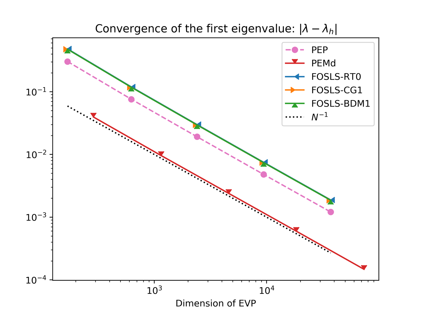
In order to confirm the convergence rates stated in Theorems 16 and 13 we first consider a square domain $\Omega=]0,1[^{2}$ where the solution of the Laplace eigenvalue problems is well known. We compare the solutions computed with a standard finite element formulation (continuous Lagrangian elements of order one), a standard mixed finite element formulation (based on lowest order Raviart–Thomas elements) and the FOSLS formulation (F1h), where we have made three choices for the space $\Sigma_{h}$ : Raviart–Thomas element, Brezzi–Douglas–Marini element, and standard Lagrangian element of lowest order; in all cases we use continuous piecewise linear polynomials for the space $U_{h}$ in the FOSLS formulation. It turns out that the results are pretty much comparable and that also in the case of the FOSLS formulation with Lagrangian elements, which is not covered by our theory, we obtain reasonable results.

Figure 1 shows various error quantities related to the approximation of the smallest eigenvalue with the considered numerical schemes.

Refer to caption — Figure 1. Error of the eigenvalue $\lambda$ and error in the $L^{2}$ -norm of $u$ , $\operatorname{\nabla}u$ , $\boldsymbol{\sigma}$ , and $\operatorname{\mathrm{div}}\boldsymbol{\sigma}$ . The used methods are the standard Galerkin formulation (PEP), the mixed formulation (PEMd), the FOSLS formulation with lowest-order Raviart–Thomas (FOSLS-RT0), continuous Lagrangian (FOSLS-CG1), and Brezzi–Douglas–Marini (FOSLS-BDM1) elements

6.2. Formulation enriched with $\operatorname{\mathbf{curl}}\boldsymbol{\sigma}$

In Subsection 2.4 we discussed how to enrich the FOSLS formulation by explicitly imposing that $\operatorname{\mathbf{curl}}\boldsymbol{\sigma}$ is zero. We observed in Subsection 4.3 that the resulting formulation is not expected to provide good results in presence of solutions where the variable $\boldsymbol{\sigma}$ is not sufficiently regular. We computed the eigenvalues of our problem on an L-shaped domain with continuous piecewise polynomials for both variables. From the convergence plots, shown in Figure 2, it is clear the first five eigenvalues have different convergence properties. In particular, the first (singular) eigenvalue is not converging; it could be actually shown that it converges optimally towards a wrong value. This is a similar behavior as what as been previously observed for other formulations involving $\operatorname{\mathrm{div}}$ and $\operatorname{\mathbf{curl}}$ of $\boldsymbol{\sigma}$ (see, for instance, [18, 16, 15].

6.3. A posteriori analysis and adaptive algorithm

The a posteriori error estimator studied in Section 5 can be naturally used in order to drive an adaptive scheme within the usual SOLVE–ESTIMATE–MARK–REFINE cycle, when Dörfler marking is adopted. We used the FOSLS formulation with Raviart–Thomas elements in order to approximate the fundamental mode of the Laplace eigenvalue problems on an L-shaped domain. Figure 3 shows the error plots as a function of the number of degrees of freedom corresponding to different choices of the Dörfler bulk parameter $\vartheta$ . Uniform refinement corresponds to the choice $\vartheta=1$ . The results show that the choice $\vartheta=0.3$ gives optimal convergence.

References

[1] A. Alonso, Error estimators for a mixed method, Numer. Math. 74 (1996), no. 4, 385–395. MR 1414415 (97g:65212)
[2] Douglas N. Arnold, Daniele Boffi, and Richard S. Falk, Quadrilateral $H({\rm div})$ finite elements, SIAM J. Numer. Anal. 42 (2005), no. 6, 2429–2451. MR 2139400
[3] I. Babuška and J. Osborn, Eigenvalue problems, Handbook of numerical analysis, Vol. II, Handb. Numer. Anal., II, North-Holland, Amsterdam, 1991, pp. 641–787.
[4] Pavel B. Bochev and Max D. Gunzburger, Least-squares finite element methods, Applied Mathematical Sciences, vol. 166, Springer, New York, 2009. MR 2490235
[5] D. Boffi, Finite element approximation of eigenvalue problems, Acta Numer. 19 (2010), 1–120. MR 2652780
[6] Daniele Boffi, Franco Brezzi, and Michel Fortin, Mixed finite element methods and applications, Springer Series in Computational Mathematics, vol. 44, Springer, Heidelberg, 2013. MR 3097958
[7] Daniele Boffi, Dietmar Gallistl, Francesca Gardini, and Lucia Gastaldi, Optimal convergence of adaptive FEM for eigenvalue clusters in mixed form, Math. Comp. 86 (2017), no. 307, 2213–2237. MR 3647956
[8] J. H. Bramble and J. E. Osborn, Rate of convergence estimates for nonselfadjoint eigenvalue approximations, Math. Comp. 27 (1973), 525–549. MR 366029
[9] James H. Bramble, Tzanio V. Kolev, and Joseph E. Pasciak, The approximation of the Maxwell eigenvalue problem using a least-squares method, Math. Comp. 74 (2005), no. 252, 1575–1598. MR 2164087
[10] Jan Brandts, Yanping Chen, and Julie Yang, A note on least-squares mixed finite elements in relation to standard and mixed finite elements, IMA J. Numer. Anal. 26 (2006), no. 4, 779–789. MR 2269196
[11] Z. Cai, T. A. Manteuffel, S. F. McCormick, and J. Ruge, First-order system $\mathscr{L}\mathscr{L}^{*}$ $({\rm FOSLL}^{*})$ : scalar elliptic partial differential equations, SIAM J. Numer. Anal. 39 (2001), no. 4, 1418–1445. MR 1870849
[12] Zhiqiang Cai and Jaeun Ku, The $L^{2}$ norm error estimates for the div least-squares method, SIAM J. Numer. Anal. 44 (2006), no. 4, 1721–1734. MR 2257124
[13] Carsten Carstensen, A posteriori error estimate for the mixed finite element method, Math. Comp. 66 (1997), no. 218, 465–476. MR 1408371 (98a:65162)
[14] M. Costabel, A coercive bilinear form for Maxwell’s equations, J. Math. Anal. Appl. 157 (1991), no. 2, 527–541.
[15] Martin Costabel and Monique Dauge, Maxwell and Lamé eigenvalues on polyhedra, Math. Methods Appl. Sci. 22 (1999), no. 3, 243–258. MR 1672271
[16] C. L. Cox and G. J. Fix, On the accuracy of least squares methods in the presence of corner singularities, Comput. Math. Appl. 10 (1984), no. 6, 463–475 (1985). MR 783520
[17] Ricardo G. Durán, Claudio Padra, and Rodolfo Rodríguez, A posteriori error estimates for the finite element approximation of eigenvalue problems, Math. Models Methods Appl. Sci. 13 (2003), no. 8, 1219–1229. MR 1998821
[18] George J. Fix and Ernst Stephan, On the finite element-least squares approximation to higher order elliptic systems, Arch. Rational Mech. Anal. 91 (1985), no. 2, 137–151. MR 806419
[19] T. Manteuffel, S. McCormick, and C. Pflaum, Improved discretization error estimates for first-order system least squares, J. Numer. Math. 11 (2003), no. 2, 163–177. MR 1987593
[20] A. I. Pehlivanov, G. F. Carey, and R. D. Lazarov, Least-squares mixed finite elements for second-order elliptic problems, SIAM J. Numer. Anal. 31 (1994), no. 5, 1368–1377. MR 1293520

	$\displaystyle\\|\operatorname{\nabla}(u-u_{h})\\|_{L^{2}(\Omega)}^{2}$	$\displaystyle}{\displaystyle\leq C\Big(\\|\boldsymbol{\sigma}-\boldsymbol{\sigma}_{h}\\|_{L^{2}(\Omega)}+\sum_{T}h_{T}\\|\operatorname{\mathrm{div}}\boldsymbol{\sigma}_{h}-\Delta u_{h}\\|_{L^{2}(\Omega)}$
		$\displaystyle+\sum_{e}h_{e}^{1/2}\\|\llbracket\operatorname{\nabla}u_{h}\cdot\mathbf{n}\rrbracket\\|_{L^{2}(e)}+h\\|\operatorname{\mathrm{div}}(\boldsymbol{\sigma}-\boldsymbol{\sigma}_{h})\\|_{L^{2}(\Omega)}\Big)$
		$\displaystyle\\|\operatorname{\nabla}(u-u_{h})\\|_{L^{2}(\Omega)}$

First order least-squares formulations for eigenvalue problems

Abstract.

1. Introduction

2. The Laplace eigenvalue problem

2.1. FOSLS formulation

Proposition 1.

Proof.

Remark 1.

2.2. The transpose FOSLS formulation

Proposition 2.

Proof.

2.3. The LL∗ formulation

Proposition 3.

2.4. Enriching the formulations with 𝐜𝐮𝐫𝐥⁡𝝈\operatorname{\mathbf{curl}}\boldsymbol{\sigma}

Remark 2.

3. Galerkin discretizazion

3.1. Approximation of the FOSLS formulations

Remark 3.

Proposition 4.

Proof.

Proposition 5.

Proof.

Proposition 6.

Proof.

Remark 4.

3.2. Approximation of the LL∗ formulation

Proposition 7.

4. Convergence analysis

4.1. Analysis of the FOSLS formulations

Proposition 8.

Lemma 9.

Proof.

Theorem 10.

Proof.

Proposition 11.

Theorem 12.

Theorem 13.

Remark 5.

Remark 6.

4.2. Analysis of the LL∗ formulation

Theorem 14.

Remark 7.

4.3. Remarks on the formulation enriched with 𝐜𝐮𝐫𝐥⁡𝝈\operatorname{\mathbf{curl}}\boldsymbol{\sigma}

5. A posteriori analysis

Theorem 15 (Reliability).

Proof.

Theorem 16 (Efficiency).

6. Numerical examples

6.1. A priori convergence: FOSLS formulation

6.2. Formulation enriched with 𝐜𝐮𝐫𝐥⁡𝝈\operatorname{\mathbf{curl}}\boldsymbol{\sigma}

6.3. A posteriori analysis and adaptive algorithm

References

2.3. The LL^∗ formulation

2.4. Enriching the formulations with $\operatorname{\mathbf{curl}}\boldsymbol{\sigma}$

3.2. Approximation of the LL^∗ formulation

4.2. Analysis of the LL^∗ formulation

4.3. Remarks on the formulation enriched with $\operatorname{\mathbf{curl}}\boldsymbol{\sigma}$

6.2. Formulation enriched with $\operatorname{\mathbf{curl}}\boldsymbol{\sigma}$