Gradient-Adjusted Neuron Activation Profiles for Comprehensive Introspection of Convolutional Speech Recognition Models

CNN are not uncommon in ASR [8]. Here, we demonstrate our model using a simple, fully-convolutional architecture based on Wav2Letter [9]. This architecture is useful for low-resource ASR model training and transfer learning [10]. Moreover, introspection methods from computer vision can easily be adapted to it [11]. For comparability, we use a pre-trained model from our previous work [12]. The 11-layer 1D-convolutional network predicts graphemes from spectrograms. The model was trained on z-normalized spectrograms, which were scaled to 128 mel-frequency bins. Whole sequence audio recordings from the LibriSpeech corpus [13] were used as training data. The acoustic model predicts sequences of graphemes, which are decoded by a CTC (CTC) beam search decoder.

Introspection describes the process of analyzing or visualizing internal structures or processes of computational models. This is of particular interest in DL (DL) models, as these work as black-boxes [2]. Several introspection techniques have been proposed, mostly in the field of computer vision [3, 4, 14]. A common way of explaining ANN is to visualize learned features by optimizing the input to maximally activate certain neurons or sets of neurons [2, 15, 16]. Optimal inputs do not always look natural. This problem can be tackled by regularizing the optimization. Another typical introspection strategy is to determine parts of the input, which are relevant for a certain prediction [3, 4, 15]. Those techniques visualize saliency maps on top of the input, which are easy to interpret. However, as those methods work on single examples, it is hard to assess the model comprehensively. Moreover, one has to choose such introspection techniques carefully, as some can be misleading [17]. More comprehensive insight into ANN is provided by analyzing representations of different classes using the complete data set. This can be done by training linear classifiers on intermediate representations [18], through CCA (CCA) of representations or by clustering class-specific neuron activations [19]. In speech, the latter type of analysis was conducted for MLP for speech-to-phoneme prediction [19, 20] and for convolutional ASR [11, 12].

For comparability with our previous work [12], we use the same model and data set. The architecture is based on Wav2Letter [9] and was trained on the LibriSpeech corpus [13]. This data set does not contain phoneme mappings. Therefore, in our earlier work, we obtained them through a grapheme-to-phoneme translation model using an attention-based encoder-decoder architecture, trained on the CMUDict (CMUDict) [21].

We introduce GradNAP as a way to compute characteristic neuron responses of an ANN to groups of inputs. GradNAP are an adaptation of the ERP technique to ANN. Our method combines and extends two of our previously described introspection methods for ASR: NAvAI (NAvAI) [11] and NAP [12]. We will first describe, how GradNAP analysis differs from our previous work. Afterwards, we explain our technique in detail.

As in our previous work, we adopt normalized averaging to obtain group-specific network responses. To preserve more information than NAP, we do not create time-independence by sorting on the time axis, but by sensitivity-based alignment like in NAvAI. Different to NAvAI, we incorporate the activation strength into the alignment, as predictions can be highly sensitive to changes in inactive neurons. On top of that, we mask out activations of low relevance for the prediction. As these improvements utilize gradients, we call our method Gradient-adjusted NAP (GradNAP).

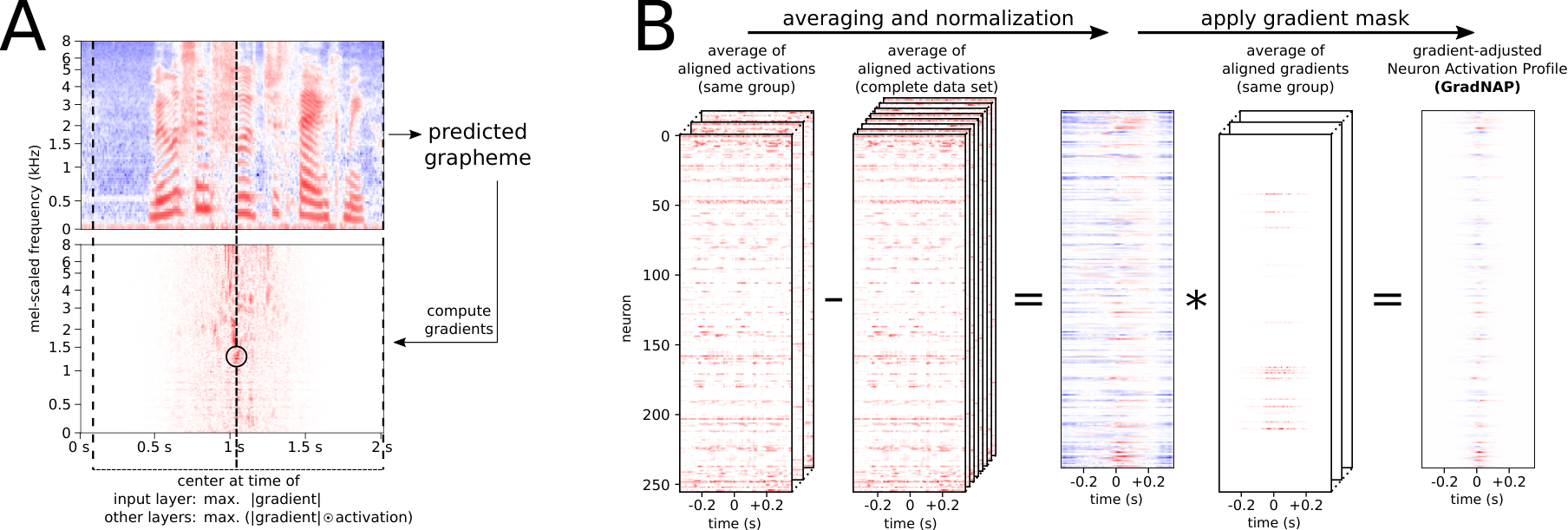
To properly apply an averaging approach, it is necessary that the different recordings are temporally aligned, similar to time-locked data in ERP analysis. To achieve this, we first center each layer’s activations and the spectrogram frames at the time of highest importance for the prediction. We refer to this step as “alignment” (Figure 1A). We compute neuron activations and sensitivity values in every layer for each spectrogram frame. Sensitivity is the gradient of a one-hot-vector for the predicted grapheme with respect to each layer’s activations. We identify importance for a prediction by strong activation with high absolute sensitivity value. Hence, we center activations at time point $t$ of maximum $(|\mathrm{gradient}|\odot\mathrm{activation})$. As zeros in z-normalized spectrograms do not represent absence of the corresponding frequency, we center spectrogram inputs at time $t$ of maximum $|\mathrm{gradient}|$, The centering is implemented by cropping. Equivalently, we center the gradients, so they remain aligned to the activations.

Figure 1B visualizes how to obtain a GradNAP in a layer. We average aligned activations and gradients over a group to obtain a group-specific profile. As some neurons show baseline activations and some information are common to all inputs, we normalize activations by subtracting the average over the complete data set. We do not normalize gradients this way, because zero-gradients would lose their meaning. Instead, we scale them to a range of $[0,1]$. Finally, we apply this gradient mask to the normalized averaged activations to obtain a GradNAP. Input layer GradNAP are computed using spectrogram frames instead of activations.

Here, we visualize GradNAP as line plots, inspired by typical action potential plots of real neurons. We compute group-responsiveness $r$ of neurons as the neuron-wise sum of absolute values in the corresponding GradNAP. A neuron $n$ can be positively or negatively responsive to a group. Hence, we multiply $r$ by the sign of the sum of GradNAP values (Equation 1).

We obtain the 5 most responsive neurons in terms of $|r_{n}|$ and compute a common optimal input. The optimization target is the joint pre-activation of those neurons at a single time point. Pre-activations of positively and negatively responsive neurons are maximized and minimized, respectively (Equation 2). We did not optimize for each responsive neuron separately, as class-specificity is distributed across multiple neurons [22].

We apply L1 and L2 regularization on the input values, scaled depending on the receptive field size $RF$ in the respective layer $l$. We scale L1 regularization by $15/RF_{l}$ and L2 by $0.1/RF_{l}$. This dependence on $RF$ avoids that regularization becomes stronger for deeper layers. Optimization is performed using Adam [23] with learning rate $0.05$ for 16 steps, initializing the input with random values from a normal distribution with $\mu=0$ and $\sigma=0.001$.

We apply hierarchical clustering with Euclidean distance and complete linkage to GradNAP of graphemes and phonemes, like in our previous work [12]. Differently, instead of using a fixed distance threshold for emergence of clusters, we apply different distance thresholds using percentiles 75% to 95% in steps of 5%. We evaluate the resulting clusterings by computing their Silhouette score [24]. This score is based on the difference between distances within clusters compared to the nearest other cluster. Moreover, we average Silhouette scores over those 5 thresholds in each layer. This ensures that the information is not specific to a particular parameter choice. We compare those results between graphemes and phonemes.

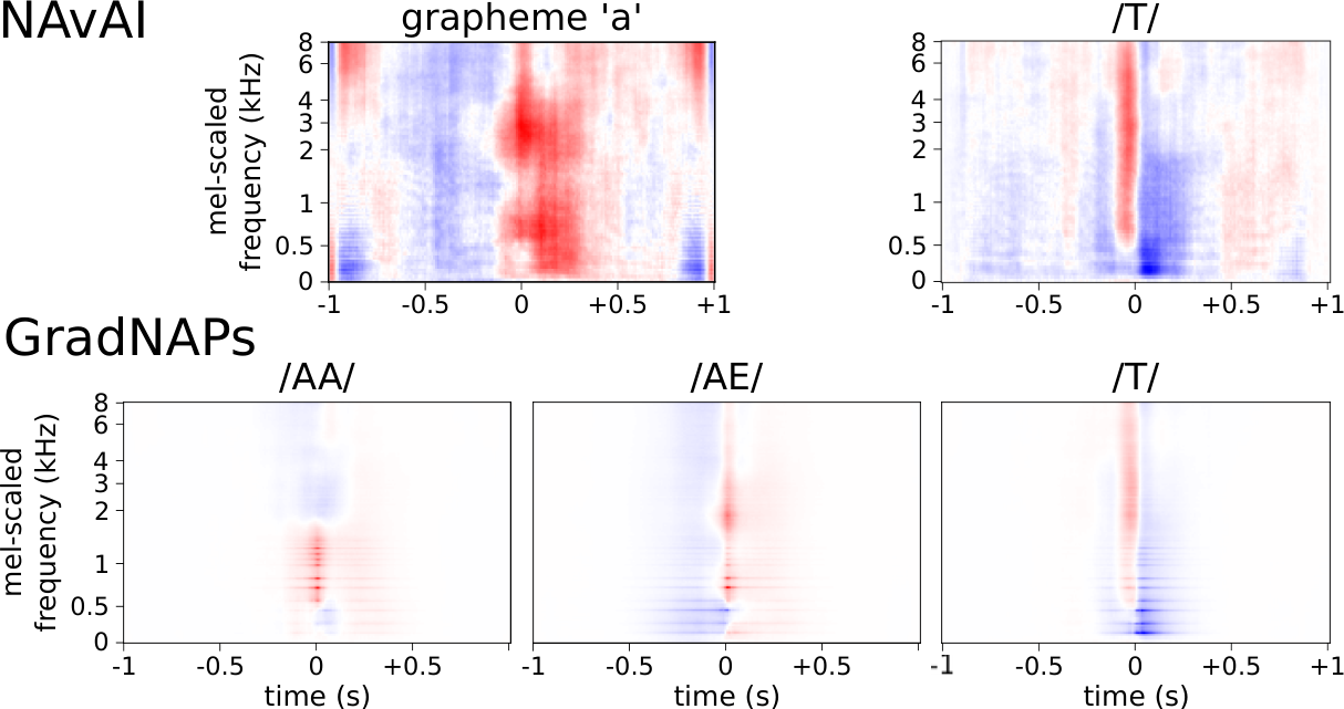
GradNAP in the input layer are an improvement of NAvAI [11]. Examples of GradNAP in the input layer compared to exemplary NAvAI results are shown in Figure 2. GradNAP in the input layer are directly interpretable. They show how the intensity of frequencies differs from the average over the complete data set. The gradient-based masking guarantees that the GradNAP only shows regions, which are important for the prediction. This advantage over NAvAI is demonstrated for /T/ in Figure 2 (right). While NAvAI shows a pattern over the whole receptive field size, the corresponding GradNAP also identified prediction-relevant parts of it.

We observe phoneme-typical patterns in input layer GradNAP (Figure 2 bottom). Phonemes /AA/ and /AE/ share a high intensity formant at around 700 Hz. A second formant is identified at around 1200 Hz and 1900 Hz for /AA/ and /AE/, respectively. The input pattern for /T/ (right) shows a change of high to low intensities of all frequencies at the alignment time. Those patterns match the expectation well. However, identified formants are spreading a wider range of frequencies. This is probably due to speaker variation. The grapheme-specific NAvAI result for a (as in [11]) is most similar to the input GradNAP for /AE/. This indicates that grapheme a was pronounced as /AE/ in the majority of the data.

In deeper layers, neuron order does not have a meaning. Therefore, corresponding GradNAP cannot be interpreted by visual inspection. An example can be seen in Figure 1B (rightmost). Instead, we visualize features by optimizing inputs for the most responsive neurons. Those results are shown in Section 4.2.

In all layers, we observed that GradNAP values become smaller and drop to 0 the further away from the alignment time. This indicates that the model did not use the complete receptive field for prediction. Thus, compressing the model in terms of choosing smaller kernel sizes, fewer filters or layers is possible.

Again inspired by neuroscience, we visualize GradNAP as neuron action potentials. Figure 3 shows GradNAP of exemplary phonemes /AE/ and /T/ in the 2^nd layer as action potential plots.

The plots show phoneme-specific neuron activations for all neurons in the same layer superimposed. The 5 most responsive neurons are highlighted with different colors (those do not represent the identity of the neuron). We observed that neuron responses to both the vowel phoneme /AE/ and the plosive /T/ are close to the center. This indicates that the network focuses on acoustic features of the phoneme, instead of correlating features in their context. Next to each action potential plot in Figure 3, the optimal input to the set of 5 most responsive neurons is shown. The optimal input for neurons which are responsive to /AE/ shows high intensities for frequencies around 700 Hz and 1900 Hz. This corresponds to the /AE/-typical formants (also in agreement with Figure 2). The visualized features for /T/-responsive neurons show several quick transitions from high to low intensities of most frequencies. As no neuron peaks twice, it is likely that the multiple occurrence of the plosive pattern is related to detecting it in different contexts. Because optimal inputs are not aligned, it is reasonable that features occur at more than one time point. This also causes repetitive patterns in optimal inputs for deeper layers, which are distinguishable but not natural. We omit them here, because unnatural feature visualization is not easily interpretable. This problem could be tackled with stronger regularization, but could also lead to misleading interpretations.

We analyze, which layers represent graphemes and phonemes best by clustering of GradNAP. In each layer, we compute Silhouette scores for cluster assignments using different distance thresholds. Higher scores correspond to more distinct clusters, indicating better representation of the respective group. Figure 4 (top) shows Silhouette scores for graphemes (left), phonemes (center) and the averages over distance thresholds for both groupings (right). Higher percentiles mostly lead to higher Silhouette scores. This is reasonable, as we expect a hierarchy of similar phonemes rather than large clusters. Surprisingly, representation quality does not consistently increase from lower to deeper layers. Silhouette scores even decrease for phonemes from the input layer to the 5^th layer. Deeper layers of the network show better clustering for phonemes than for graphemes over all distance thresholds. The highest Silhouette score can be observed for phonemes in the 9^th layer. However, the corresponding clusters are large and do not separate phonemic categories. Layers 10 and 11 have a much larger number of neurons than the others. This results in differently distributed distance matrices, which probably causes the drop of cluster quality from layer 9 to layer 10.

Silhouette scores indicate that in higher layers, phonemes are better represented than graphemes. However, they are not suitable for detecting the exact layer, where clusters of meaningful phonemic categories emerge. This indicates that phoneme similarity is not the strongest factor for distinguishing neuron responses. Nevertheless, we observe similar phonemic categories in clusterings from the 10^th layer on, which is shown in Figure 4 (bottom). In an earlier work, we performed clustering analysis of NAP [12]. We confirm the prior finding, that phonemic categories are represented well from the 10^th layer on and that the phoneme clustering is identifying more sub-categories. However, the differences between grapheme and phoneme clustering are smaller than in our earlier work. Most likely, this is an effect of gradient masking, which scales down a lot of prediction-irrelevant values.

References

- [1] Christian Szegedy, Wei Liu, Yangqing Jia, Pierre Sermanet, Scott Reed, Dragomir Anguelov, Dumitru Erhan, Vincent Vanhoucke, and Andrew Rabinovich, “Going deeper with convolutions,” in Proceedings of the IEEE conference on computer vision and pattern recognition, 2015, pp. 1–9.
- [2] Jason Yosinski, Jeff Clune, Anh Nguyen, Thomas Fuchs, and Hod Lipson, “Understanding neural networks through deep visualization,” arXiv preprint arXiv:1506.06579, 2015.
- [3] Matthew D Zeiler and Rob Fergus, “Visualizing and understanding convolutional networks,” in European conference on computer vision. Springer, 2014, pp. 818–833.
- [4] Ramprasaath R. Selvaraju, Abhishek Das, Ramakrishna Vedantam, Michael Cogswell, Devi Parikh, and Dhruv Batra, “Grad-CAM: Visual explanations from deep networks via gradient-based localization,” arXiv preprint arXiv:1610.02391, 2016.
- [5] Andreas Krug and Sebastian Stober, “Adaptation of the event-related potential technique for analyzing artificial neural networks,” in Cognitive Computational Neuroscience (CCN), 2017.
- [6] Scott Makeig, Julie Onton, et al., “ERP features and EEG dynamics: an ICA perspective,” in Oxford handbook of event-related potential components, pp. 51–87. Oxford, 2009.
- [7] Steven J. Luck, “An Introduction to the Event-Related Potential Technique,” Monographs of the Society for Research in Child Development, vol. 78, no. 3, pp. 388, 2005.
- [8] Ossama Abdel-Hamid, Abdel-rahman Mohamed, Hui Jiang, Li Deng, Gerald Penn, and Dong Yu, “Convolutional neural networks for speech recognition,” IEEE/ACM Transactions on audio, speech, and language processing, vol. 22, no. 10, pp. 1533–1545, 2014.
- [9] Ronan Collobert, Christian Puhrsch, and Gabriel Synnaeve, “Wav2letter: an end-to-end convnet-based speech recognition system,” arXiv preprint arXiv:1609.03193, 2016.
- [10] Julius Kunze, Louis Kirsch, Ilia Kurenkov, Andreas Krug, Jens Johannsmeier, and Sebastian Stober, “Transfer learning for speech recognition on a budget,” in Proceedings of the 2nd Workshop on Representation Learning for NLP. 2017, pp. 168–177, Association for Computational Linguistics.
- [11] Andreas Krug and Sebastian Stober, “Introspection for convolutional automatic speech recognition,” in Proceedings of the 2018 EMNLP Workshop BlackboxNLP: Analyzing and Interpreting Neural Networks for NLP, 2018, pp. 187–199.
- [12] Andreas Krug, René Knaebel, and Sebastian Stober, “Neuron activation profiles for interpreting convolutional speech recognition models,” in Proceedings of the 2018 NeurIPS Workshop IRASL: Interpretability and Robustness for Audio, Speech, and Language, 2018.
- [13] Vassil Panayotov, Guoguo Chen, Daniel Povey, and Sanjeev Khudanpur, “Librispeech: an ASR corpus based on public domain audio books,” in Acoustics, Speech and Signal Processing (ICASSP), 2015 IEEE International Conference on. IEEE, 2015, pp. 5206–5210.
- [14] Sebastian Bach, Alexander Binder, Grégoire Montavon, Frederick Klauschen, Klaus-Robert Müller, and Wojciech Samek, “On pixel-wise explanations for non-linear classifier decisions by layer-wise relevance propagation,” PloS one, vol. 10, no. 7, pp. e0130140, 2015.
- [15] Dumitru Erhan, Yoshua Bengio, Aaron Courville, and Pascal Vincent, “Visualizing higher-layer features of a deep network,” University of Montreal, vol. 1341, no. 3, pp. 1, 2009.
- [16] Alexander Mordvintsev, Christopher Olah, and Mike Tyka, “Inceptionism: Going deeper into neural networks,” Google Research Blog. Retrieved June, vol. 20, no. 14, pp. 5, 2015.
- [17] Julius Adebayo, Justin Gilmer, Michael Muelly, Ian Goodfellow, Moritz Hardt, and Been Kim, “Sanity checks for saliency maps,” in Advances in Neural Information Processing Systems, 2018, pp. 9525–9536.
- [18] Guillaume Alain and Yoshua Bengio, “Understanding intermediate layers using linear classifier probes,” arXiv preprint arXiv:1610.01644, 2016.
- [19] Tasha Nagamine, Michael L Seltzer, and Nima Mesgarani, “Exploring how deep neural networks form phonemic categories,” in Sixteenth Annual Conference of the International Speech Communication Association, 2015.
- [20] Tasha Nagamine and Nima Mesgarani, “Understanding the representation and computation of multilayer perceptrons: A case study in speech recognition,” in International Conference on Machine Learning, 2017, pp. 2564–2573.
- [21] Kevin Lenzo, “The CMU pronouncing dictionary,” Carnegie Melon University, 2007.
- [22] Ari S Morcos, David GT Barrett, Neil C Rabinowitz, and Matthew Botvinick, “On the importance of single directions for generalization,” arXiv preprint arXiv:1803.06959, 2018.
- [23] Diederik P Kingma and Jimmy Ba, “Adam: A method for stochastic optimization,” arXiv preprint arXiv:1412.6980, 2014.
- [24] Peter J Rousseeuw, “Silhouettes: a graphical aid to the interpretation and validation of cluster analysis,” Journal of computational and applied mathematics, vol. 20, pp. 53–65, 1987.