Architecture of three-planet systems predicted from the observed protoplanetary disk of HL TauJournal: ApJ

For a planet within a disk, in addition to the gravitational forces exerted by the central star and other planets, the planet will experience forces due to planet-disk interactions. Consider the forces acting on the i-th planet, the equation of motion can be written as

where $\boldsymbol{r}_{i}$ is the position vector of the i-th planet. The $\boldsymbol{f}$ notations on the right hand side of the equation are respective forces per unit mass exerting on the i-th planet. We assume the planets to be co-planar, and thus $\boldsymbol{r}_{i}$ can be replaced by the position vector $\boldsymbol{R}_{i}(R_{i},\phi_{i})$ in cylindrical coordinate system. We use $\boldsymbol{R}$ to denote the cylindrical position vector unless stated otherwise.

The first term, $\boldsymbol{f}_{\text{grav}}$, of the right-hand-side of equation (1) denotes gravitational force exerted by the central star and other planets, and is given by (Murray & Dermott 2000, e.g.):

where $M_{*}$ is the mass of the central star, $M_{i}$ is the mass of the $i$-th planet, $R=\lvert\boldsymbol{R}\rvert$, and $\mathcal{G}$ is the gravitational constant.

The second term, $\boldsymbol{f}_{a,i}$, denotes the force driving the migration of planet. A planet with index $i$ embedded in the disk experiences an effective torque $\Gamma_{i}$, and migrates inwards. To describe the motion, it is convenient to introduce an e-folding inward migration time-scale $\tau_{a,i}$:

where $a_{i}$ is the semi-major axis of the $i$-th planet. In the case of a co-planar and near circular orbit, $|\boldsymbol{R}_{i}|\approx a_{i}$, and equation (4) reduces to

in terms of the angular momentum $L_{i}$ and the torque $\Gamma_{i}$ acting on the planet from the disk. Thus, the effective migration force, $\boldsymbol{f}_{a,i}$, is simply given by

The disk tends to circularise a planetary orbit. Similarly as equation (4), we define the eccentricity damping time-scale, $\tau_{e,i}$. Following Lee & Peale 2002; Kley et al. 2004, we further assume the following expression:

where $C$ is a constant, and $h_{i}/R_{i}$ is the aspect ratio of the disk at the location of the $i$-th planet. Then the eccentricity damping force is computed as

where $\hat{\mathbf{\boldsymbol{\ell}}}_{i}$ is the unit vector of the specific angular momentum of the $i$-th planet. (See Appendix A of Lee & Peale 2002).

In section III.1 we have defined the migration time-scale $\tau_{a,i}$ to capture the physics of the migration process. In practice, we adopt an empirical model $\tau_{a,i}$ by Kanagawa et al. 2018. Since this is one of the most important processes that we implement in the current simulation, we summarise the explicit formulae in this subsection.

Kanagawa et al. 2018 performed two-dimensional hydrodynamical simulations, and investigated the planetary migration by varying disk parameters. They found that the migration slows down as the gap becomes deeper. The depth of the gap, defined as the ratio between the minimum bottom density of the gap $\Sigma_{{\rm min},i}$ and the surface density of the unperturbed vicinity $\Sigma_{g}(R_{i})$, can be characterised by a dimensionless factor $K_{i}$ as

where

A small value of $K_{i}$ corresponds to the case of a small planet mass ($M_{i}$), in which the planetary migration is in Type I regime. As the planet mass grows due to accretion from disk, the gap depth and therefore $K_{i}$ gradually increase, and the migration becomes slower (Type II regime).

Adopting this gap parametrisation, Kanagawa et al. 2018 found the following empirical expression of $\tau_{a,i}$ that incorporates the slower migration for the deeper gap:

In equation (11), $\gamma_{C,i}=\Gamma_{C,i}/\Gamma_{0,i}$ and $\gamma_{L,i}=\Gamma_{L,i}/\Gamma_{0,i}$, where $\Gamma_{C,i}$, $\Gamma_{L,i}$, and $\Gamma_{0,i}$ denote the co-rotation, Lindblad, and characteristic torque for the $i$-th planet, respectively. The characteristic torque $\Gamma_{0,i}$ is defined as

Here $K_{t}$ is the co-rotational cut-off value of $K_{i}$, $\Omega_{K,i}$ is the Keplerian angular velocity of the $i$-th planet, and $\tau_{0,i}$ is the characteristic time-scale defined as $\tau_{0,i}=L_{i}/(2\Gamma_{0,i})$. For a deep gap ($K_{i}\gg K_{t}$), equation (11) reduces to

which reflects the fact that the migration becomes slower for a deeper gap.

We further adopt the following explicit expressions for the dimensionless torques, which are derived by Paardekooper et al. 2010 assuming that the disk is locally isothermal:

where $s=-\ln\Sigma_{g}/\ln R$ and $\beta=-\ln T/\ln R$ are the power-law indices of the surface density and temperature profiles. The dimensionless factor $b_{i}$ was originally introduced by Paardekooper et al. 2010. The value of $b_{i}$ is fixed to be $2/3$ in our simulation, following Kanagawa et al. 2018.

Tanigawa & Tanaka 2016 studied the mass growth of a giant planet and obtained a semi-empirical model of the gas accretion rate onto the planet, which is in reasonable agreement with the results of hydrodynamic simulations. We adopt their model of planetary accretion and hereby summarise key expressions relevant to our simulation.

The model of Tanigawa & Tanaka 2016 states that the accretion rate of the $i$-th planet, $\dot{M}_{i}$, can be expressed in terms of the accretion area per unit time $D_{i}$ and the disk surface density of the accretion channel $\Sigma_{{\rm acc},i}$ at its location $R_{i}$. Since the gas accretion only takes place at the close vicinity of the planet (gas can accrete at around two Hill radii from the planet), we can replace $\Sigma_{\rm acc,i}$ to $\Sigma_{\rm min,i}$ given by Equation (9). $\dot{M}_{i}$ is then written as²² 2 Instead of Equation (9), Tanigawa & Tanaka 2016 adopt a slightly different formula $\Sigma_{\rm min,i}=1/(1+0.034K_{i})$. This difference does not change our main results.

We compute $\dot{M}_{i}$ iteratively for a given $\dot{M}_{\rm glob}$ and other planetary configuration.

The planetary migration and accretion require a disk profile model. For a static and axisymmetric disk surrounding a star, the surface density profile is given by

where $\dot{M}_{*}$ is the stellar accretion rate, and $\nu$ is the kinematic viscosity (Pringle 1981).

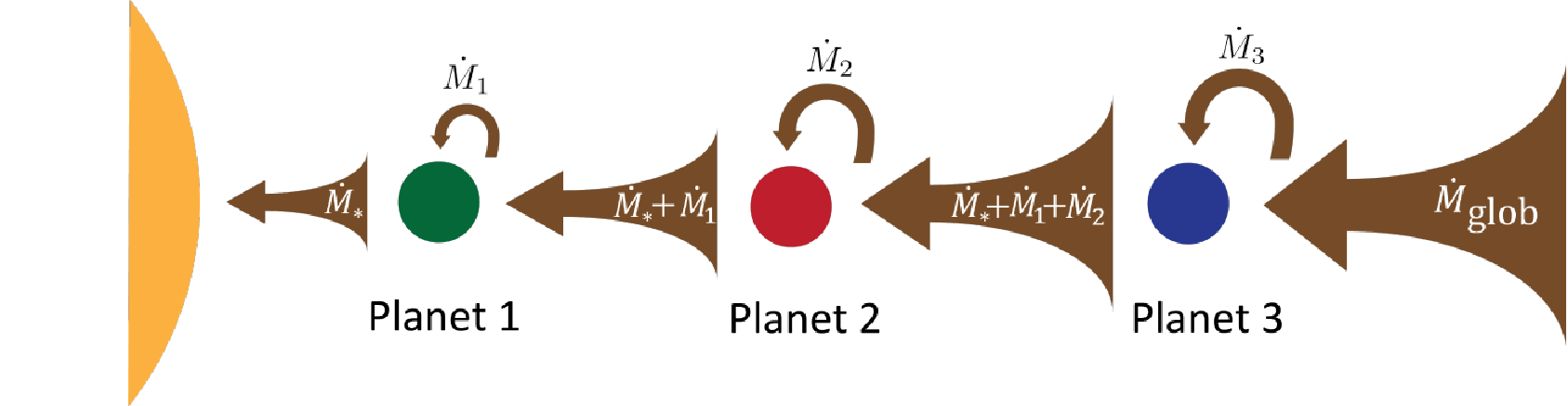
Equation (18) assumes that the disk mass accretes on the central star only and neglects the accretion on planets. Tanigawa & Tanaka 2016 incorporates the mass accretion onto a single planet by approximating the planet as a sink for mass and angular momentum within an inward disk mass flow. We generalise their model for a multi-planetary system, as schematically illustrated in Figure 1.

To be more specific, we consider a quasi-steady disk with the $i$-th planet located at $R_{i}$ with its accretion rate $\dot{M}_{i}$ ($i=1,2,\cdots,N$). We define a global accretion rate as the sum of all the accretion rates:

Moreover we assume that the initial value of $\dot{M}_{\rm glob}$ only depends on global parameters of the disk, which are unaffected by the migration and accretion of the planets (see later section III.5). Then the surface density profile $\Sigma_{\rm g}(R)$ between the $n$-th and $(n+1)$-th planets ($R_{n}\leq R<R_{n+1}$) is modelled as

(see Appendix A). The above formula shows that the surface density profile couples with the migration and accretion of the planet. Particularly, when $R$ is large, the profile reduces to the form of equation (18), i.e., $\Sigma_{g}(R)\simeq\dot{M}_{\rm glob}/(3\pi\nu)$.

Since the location that we consider is far away from the star ($R\gg R_{*}$), the bracket of the first term on the right-hand-side of equation (20) is unity in practice. If the position and mass of each planet are specified, we can first express the accretion rate of each planet in terms of $\dot{M}_{\rm glob}$ by evaluating equation (20) at each $R_{i}$ and then substituting to equation (16). Once $\dot{M}_{\rm glob}$ is given, we can then compute the explicit mass accretion rate of each planet as well as surface density at an arbitrary distance $R$.

We take account of the gas removal from the disk, simply adopting an exponentially decaying model:

where $\dot{M}_{\rm glob}^{\rm ini}$ is the initial value of the global mass acrretion rate, and $\tau_{disk}$ is the e-folding decay time of the disk mass.

Due to the large uncertainty of the disk lifetime, we treat $\tau_{\rm disk}$ as a free parameter in the simulation and consider $\tau_{\rm disk}=1$, 2 and 3 Myr. Note that for simplicity, the surface density profile given by equation (20) does not include the shape of the gap induced by the planet. Equation (20) gives $\Sigma_{\rm g}(R_{i})$ in equation (9).

We evolve each system numerically including the planet-disk interaction and mass accretion on the basis of the public $N$-body code REBOUND (Rein & Liu 2012) and its extension REBOUNDx. We choose an adaptive time-step integrator integrator ias15 (Rein & Spiegel 2014). Within the framework of REBOUNDx, we implement additional forces and modify the disk mass according to the surface density.

Our simulation starts from initial conditions following the observed structure of the HL Tau disk (see section II). Table 1 summarizes the disk initial conditions that we adopted. We take $0.105\text{\,}\mathrm{M}_{\odot}$ as the disk mass from Kwon et al. 2015 and set the inner edge and outer edge to be $10\text{\,}\mathrm{a}\mathrm{u}$ and $80\text{\,}\mathrm{a}\mathrm{u}$. For simplicity, we assume the stellar mass of HL Tau is $1\text{\,}\mathrm{M}_{\odot}$.

We use a simple power law model to characterise the vertical geometry of the HL Tau disk. The aspect ratio is expressed as

where $f$ is the flaring index. We consider five flaring indices from $0.15$ to $0.35$. The reference aspect ratio at $1\text{\,}\mathrm{a}\mathrm{u}$ is fixed to be $0.03$, which is roughly consistent with the values used in previous studies (Dipierro et al. 2015; Kanagawa et al. 2015, e.g.).

We assume that the disk viscosity $\alpha$ does not vary with time and position. Considering the low turbulence level suggested by the dust settling, we follow Pinte et al. 2015 and take the fiducial $\alpha$ value to be $3\text{\times}{10}^{-4}$. We also consider $\alpha=$ $2\text{\times}{10}^{-4}$, $4\text{\times}{10}^{-4}$, $5\text{\times}{10}^{-4}$, and $6\text{\times}{10}^{-4}$ so as to see the dependence on $\alpha$.

We normalise the initial global accretion rate $\dot{M}_{\rm glob}^{\rm ini}$ using the initial disk mass calculated from the unperturbed surface density profile(equation 18)

Therefore,

where $\nu_{\rm 1au}=\alpha\left(\frac{h}{R}\right)^{2}_{\rm 1au}\Omega_{K,$1\text{\,}\mathrm{a}\mathrm{u}$}$. Note that in the present simulation, we adopt $M_{\rm disk}^{\rm ini}=0.105M_{\odot}$, which is the initial mass of the disk within the range from $R_{\rm in}=$10\text{\,}\mathrm{a}\mathrm{u}$$ to $R_{\rm out}=$80\text{\,}\mathrm{a}\mathrm{u}$$. In the fiducial case, $\dot{M}_{\rm glob}^{\rm ini}=$3.82\text{\times}{10}^{-9}\text{\,}\mathrm{M}_{\odot}\mathrm{y}\mathrm{r}^{-1}$$.

Table 2 summarises the planet-related initial conditions. 68 interpreted the HL Tau disk substructure as the existence of four or five planets. Since hydrodynamic simulations (Dipierro et al. 2015; Jin et al. 2016) have shown that the major substructures of the HL tau disk can be well reproduced by three planets, we consider three planets initially located at $13.2\text{\,}\mathrm{a}\mathrm{u}$, $32.3\text{\,}\mathrm{a}\mathrm{u}$ and $73.7\text{\,}\mathrm{a}\mathrm{u}$, corresponding to the first, second and fourth planets in 68. For reference, the mid-plane disk temperature at the location of each planet is $45\text{\,}\mathrm{K}$, $29\text{\,}\mathrm{K}$ and $19\text{\,}\mathrm{K}$ from inner to outer, if the temperature at $13.2\text{\,}\mathrm{a}\mathrm{u}$ gap is taken as $45\text{\,}\mathrm{K}$ (Table 2, Pinte et al. 2015) and the flaring index is the fiducial value $0.25$.

We assume that the planets are co-planar and initially in near-circular orbits by setting the initial eccentricity to be ${10}^{-7}$ for all the three planets. The adopted planetary masses are given from the width of the gap to the planetary mass using an empirical formula following Kanagawa et al. 2016. We choose the planetary masses to be $0.77\text{\,}\mathrm{M}_{\mathrm{J}}$, $0.11\text{\,}\mathrm{M}_{\mathrm{J}}$, and $0.27\text{\,}\mathrm{M}_{\mathrm{J}}$ for our fiducial model of $\alpha=$ $3\text{\times}{10}^{-4}$, and scale them by $\propto\alpha^{1/2}$ (See Equation (5) of Kanagawa et al. 2015 and also Table 2).

As shown in Table 1, we perform $5\times 3\times 5=75$ simulation runs by varying disk parameters. The simulation stops at $t=3\tau_{\rm disk}$ when the gas component of the disk is sufficiently removed from the system.

Figure 2 shows an example of planetary evolution with fiducial parameters: flaring index $f=0.25$, disk lifetime $\tau_{\rm disk}=$2\text{\,}\mathrm{M}\mathrm{y}\mathrm{r}$$ and viscosity $\alpha=$3\text{\times}{10}^{-4}$$. In $6\text{\,}\mathrm{M}\mathrm{y}\mathrm{r}$, orbits of planets $1,2,3$ shrink from $(13.2,32.3,73.7)$\mathrm{a}\mathrm{u}$$ to $(11.6,22.5,40.7)$\mathrm{a}\mathrm{u}$$, respectively, which remain widely separated. Their masses increase from $(0.77,0.11,0.27)$\mathrm{M}_{\mathrm{J}}$$ to $(1.6,2.3,4.6)$\mathrm{M}_{\mathrm{J}}$$. The relation between semi-major axis and mass agrees with the result of Tanaka et al. 2019 who have investigated the evolution of a single planet within the disk.

Due to the large initial mass and the low surface density, the innermost planet (Planet 1) barely migrates throughout the disk stage. The outer two planets (Planet 2 and 3) quickly grow and migrate inward for the first $0.5\text{\,}\mathrm{M}\mathrm{y}\mathrm{r}$. As the mass of planets keep growing, the migration of the two planets gradually slows down, and they eventually approach their final positions as the disk surface density decays.

Over the entire migration, eccentricities of the three planets are very small since the slow Type II migration does not lead to any close encounter between the planets. The eccentricities of all three planets are below $0.01$ for $t<$2\text{\,}\mathrm{G}\mathrm{y}\mathrm{r}$$. For Planet 2, there is a slight excitation of eccentricity at around $3.6\text{\,}\mathrm{M}\mathrm{y}\mathrm{r}$ due to the approach of Planet 3. Even after the excitation, eccentricities of Planet 2 and 3 fluctuate around $0.025$ and $0.015$ and nearly stop growing.

The migration time-scales in Figure 2 indicate that the outer planet initially migrates faster than the inner planet. In the first $\mathrm{M}\mathrm{y}\mathrm{r}$, the migration time-scales of Planet 2 and Planet 3 gradually increase, as their gaps become deeper due to the mass growth. The accretion rates of the outer planets also drop, so more mass can flow inside and boost the migration of Planet 1, which explains the decrease of the migration time-scale of Planet 1. The migration time-scales of all the three planets exceed $10\text{\,}\mathrm{M}\mathrm{y}\mathrm{r}$ at $t=$2\text{\,}\mathrm{M}\mathrm{y}\mathrm{r}$$. They eventually exceed $100\text{\,}\mathrm{M}\mathrm{y}\mathrm{r}$ at $t=$6\text{\,}\mathrm{M}\mathrm{y}\mathrm{r}$$, and their migration ceases practically.

Figure 3 plots the global surface density profile (cf. equation 20) at four different epochs of the fiducial run, while Figure 4 is the evolution of the surface density evaluated at the location of each planet. At $t=0$, the strong mass accretion onto planets 2 and 3 creates steep bumps on the density profile, and the surface density around Planet 1 is quenched to less than $1\text{\,}\mathrm{\%}$ of the unperturbed value. As Planets 2 and 3 continue to grow, their accretion rates drop as $\dot{M}_{i}\propto M_{i}^{-2/3}$. Thus the mass flows through the outer planets and accretes inward preferentially on planet 1 and the star. At $t=$2\text{\,}\mathrm{M}\mathrm{y}\mathrm{r}$$, the planetary system becomes more closely packed and accretion rates of all the planets drop. As a result, density bumps around the planets almost vanish, while the density at the vicinity of each planet reaches the maximum at this epoch. At $t=$6\text{\,}\mathrm{M}\mathrm{y}\mathrm{r}$$, the density bumps become further negligible and the surface densities at three planets become nearly identical.

Figure 5 illustrates the configurations of the planetary systems at $3\tau_{\rm disk}$ with different disk parameters. For each plot, we vary only one free parameter while the other two are fixed as their fiducial values. Overall the mass of the outer planet is larger than that of inner one, because the outer planet grows faster than the inner one. The gas accretion onto the outer planet decreases the gas surface density around the inner planets. Because of the lower gas density, the migration and mass growth of the inner ones are suppressed until the gas accretion onto the outer planet becomes small due to the formation of the deep gap. This is why the evolution of the inner planet is less sensitive to the disk parameters compared to the outer planet. The final semi-major axis and planetary mass change monotonically with the value of each parameter.

When the flaring index $f$ increases from $0.15$ to $0.35$, the final semi-major axis decreases and final mass increases. As the flaring index become larger, the aspect ratio of the disk increases quickly with radii, resulting in a much shallower gap since the gap depth is sensitive to the aspect ratio to the fifth power (see equations 9 and 10). While the ratio of Lindblad torque decreases with the flaring index since $T\propto R^{-(1-2f)}$ and $\Sigma\propto R^{-(0.5+2f)}$ (see equation 15), the effects caused by a shallower gap dominates both the migration time-scale (see equation 13) and accretion rate. Consequently, the planets experience stronger migration and accretion, and eventually move further inward and become more massive. This effect is stronger at large radii, and hence the outermost planet is most affected, as shown by Figure 5.

When $\tau_{disk}$ increases from $1\text{\,}\mathrm{M}\mathrm{y}\mathrm{r}$ to $3\text{\,}\mathrm{M}\mathrm{y}\mathrm{r}$, the final semi-major axis decreases and final mass increases monotonically. Since $\tau_{\rm disk}$ is basically a disk lifetime, the above trend is easily understood as planets in a long-lived disk simply have longer time for migration and accretion.

Finally, a higher viscosity implies that planets experience stronger migration and accretion, as evidenced by the decreasing semi-major axis and increasing final mass. Physically, it is because the angular momentum transfer becomes more efficient with a higher viscosity. A more quantitative discussion can be made from equation (10), which is similar to the explanation of flaring index dependence. Since the diffusion time-scale is proportional to $\nu^{-1}\propto\alpha^{-1}$, a larger value of $\alpha$ leads to a faster gas diffusion, resulting in a shallower gap carved by a planet with the same given mass, i.e., the $K$ value is smaller. Thus the migration time-scale is shorter and migration is faster. The mass accretion dependence on $K$ is understood similarly: the accretion density $\Sigma_{acc}$ is higher for a shallower gap, and therefore a planet grows factor with a higher accretion rate and becomes more massive.

We find that 74 out of our $75$ runs remain stable until the end of the disk gas removal at $3\tau_{\rm disk}$, but the remaining run with $f=0.35$, $\tau_{\rm disk}=$3\text{\,}\mathrm{M}\mathrm{y}\mathrm{r}$$, and $\alpha=$6\text{\times}{10}^{-4}$$ turns out to be unstable before the epoch. In this case, the innermost Planet 1 is ejected due to gravitational scattering, and the remaining Planet 2 and 3 are in fairly eccentric orbits($e_{2}=0.55,e_{3}=0.21$). We therefore exclude this single unstable case in our follow-up analysis. Nevertheless, this unstable case stresses the importance of the planet-planet interaction even before the dispersal of the disk, which is absorbed in our N-body approach. When planets are close to each other, particularly inside the resonance overlapping region, planet-planet interactions can couple with the planet-disk interactions and play an important role in shaping the stability of the configuration.

We continue evolving the $74$ systems from the final planetary configurations at $3\tau_{\rm disk}$ of the previous disk stage using purely $N$-body simulation after the disk dispersal. When one of the planets is ejected from the system or collide with star/other planet, we stop the simulation and mark the run unstable. Otherwise the system is integrated up to $10\text{\,}\mathrm{G}\mathrm{y}\mathrm{r}$. The simulation runs are effectively 2D simulation since no inclination has been introduced throughout our simulations.

Figure 6 shows the orbital evolution of the planets in our fiducial case after the disk dispersal. Clearly there is no significant change in the semi-major axis and eccentricity of the planet during $10\text{\,}\mathrm{G}\mathrm{y}\mathrm{r}$. We also confirmed that the majority of the systems ($69$ out of $74$) remain stable until $10\text{\,}\mathrm{G}\mathrm{y}\mathrm{r}$ as in the case shown in Figure 6.

A low fraction of unstable systems may imply that most of the planetary configuration achieved through physical disk-planet evolution is indeed stable. This is in contrast to the fact that a significant fraction of numerical simulations exhibit unstable outcomes, most likely due to their relatively artificial initial conditions. Our result indicates that the production of misaligned planets and Hot Jupiters via the instability channel is rather inefficient, at least for the HL Tau disk.

The remaining $5$ systems become unstable within $0.004\text{\,}\mathrm{G}\mathrm{y}\mathrm{r}$ to $5.7\text{\,}\mathrm{G}\mathrm{y}\mathrm{r}$. We find that the instability time is extremely sensitive to the numerical treatment because of the chaotic nature of such systems, and even a tiny numerical truncation error could result in a $50\text{\,}\mathrm{\%}$ change of the instability time. The precise value of the instability time can be trusted roughly within an order of magnitude. More detailed discussions on the instability is given in section V.1 below.

The stability criterion of a multi-planetary system has been extensively investigated. In particular, a number of previous work (Gladman 1993; Chambers et al. 1996; Marzari & Weidenschilling 2002; Quillen 2011; Tamayo et al. 2016; Wu et al. 2019, e.g.) pointed out on the basis of the Hill stability argument that a mutual orbital separation of planets plays an important role in their long-term stability. However, when the planetary mass is large, the mean resonance becomes important and those empirical relations based on mutual Hill radius are not directly applicable. We found that the instability time predictions given by Chambers et al. 1996 and Marzari & Weidenschilling 2002 significantly underestimate the lifetime of our simulated systems. For instance, the criterion given by Marzari & Weidenschilling 2002 predicts half of the systems to be unstable, though most of the systems are stable in our simulations. This discrepancy is originated from the planetary mass dependence of the stability criterion.

Morrison & Kratter 2016 performed a series of simulations with three and five equal-mass planets and found that the mean resonance overlap is a better measure of the orbital stability in the high mass regime larger than Jupiter. On the basis of their argument, we consider the following empirical log-linear relation between an orbital instability time $T_{\rm ins}$ and a dimensionless orbital spacing $\zeta$:

where $P_{\rm inner}$ is the orbital period of the inner-most planet, $M_{p}$ is the planetary mass, $\delta a_{{\rm ro},i}$ is the separation where two first-order mean resonances overlap, and $c$ and $d$ are numerical constants.

Note that the initial conditions of the simulations of Morrison & Kratter 2016 are such that $\zeta_{i}$ are independent of $i$ for a given system, and thus $\zeta_{\rm min}=\zeta_{i}$. Then we fit equation (25) to their result (left panel of their Figure 3 with three equal-mass planets), and found that $c\approx 15.3$ and $d\approx-16.1$ for planets more massive than ${10}^{-3}\text{\,}\mathrm{M}_{\odot}$ reproduce their data roughly within one order-of-magnitude.

Since our systems consist of three unequal-mass planets, and $\zeta_{i}$ depend on $i$, we cannot directly adopt equation (25) for the stability condition. Deck et al. 2013 found the same relation hold if the mass ratio in the original $\delta a_{{\rm ro},i}$ is replaced by the sum of the mass ratios of two planets, i.e., $\delta a_{{\rm ro},i}^{\prime}$. We compared both scaling factors and found $\delta a_{{\rm ro},i}^{\prime}$ is more consistent with our results with unequal planetary mass. Thus we extrapolate equation (25) and rewrite it in terms of $\delta a_{{\rm ro},i}^{\prime}$ as follows:

In the above expression, $a_{\rm inner}$ is the semi-major axis of the innermost planet evaluated at the initial epoch for the $N$-body simulation (i.e., at the end of the disk-planet interaction run), and

Figure 7 plots $\zeta_{min}$ against the $a_{\rm inner}$ for 74 runs. Circles indicate 69 systems that are stable until $t=$10\text{\,}\mathrm{G}\mathrm{y}\mathrm{r}$$, while the remaining 5 systems (crosses) become unstable within the integration time. As a reference, equation (29) predicts that $62$ systems are stable, and our simulation confirmed that $59$ out of the $62$ systems ($95.2\%$) are indeed stable. On the other hand, among the $12$ systems that are predicted to be unstable within $10\text{\,}\mathrm{G}\mathrm{y}\mathrm{r}$, only $2$ systems become unstable, indicating that equation (29) systematically underestimates the instability time to some extent. Although the actual instability time can deviate up to two or three orders of magnitude from the predicted line, equation (29) outperforms other criteria and is roughly consistent with our result that most of systems are stable within $10\text{\,}\mathrm{G}\mathrm{y}\mathrm{r}$.

The stability of systems emerging from the HL Tau disk may be understood as well in the context of the mean-motion resonance (MMR) capture during a convergent migration (Mustill & Wyatt 2011; Goldreich & Schlichting 2014; Deck & Batygin 2015; Tamayo et al. 2017). Obertas et al. 2017 found that the stability of a planetary system is enhanced if a pair of planets are in a near-resonant state. Tamayo et al. 2017 performed simulations for the TRAPPIST-1 planetary system, and concluded that the disk migration can produce a resonant chain of planets, which significantly stabilises the system.

Motivated by these studies, we plot the histogram of period ratios between adjacent planets, $P_{2}/P_{1}$ and $P_{3}/P_{2}$, at the initial epoch (Figure 8). The period ratios fall within the range from $2.1$ to $3.0$. The minimum period ratio is clearly above $2.0$, indicating that no planet pair has ever entered the strongest first-order resonance region. The cut-off implies the existence of a strong co-migration between two planets; when the outer planet approaches the inner planet from outside of 2:1 period ratio, the inner planet is forced to migrate together, which prevents the planet pair from further approaching and entering the first-order MMR region.

The period ratios of the two adjacent pairs also exhibit different statistical distributions. The period ratios of the outer pair ($P_{3}/P_{2}$) are widely distributed between $2.1$ and $2.9$ range, while those of the inner pair ($P_{2}/P_{1}$) are in a narrow range between $2.5$ and $2.8$ with a peak at $2.6$. These distributions indicate that the outer pairs are more closely-packed than the inner pairs on average. One possible explanation is that the period ratio is determined by the migration speed difference of the pair. In the case of the outer pair, the faster migration speed of Planet 3 allows Planet 3 to reach the region closer to the 2:1 resonance before the co-migration starts. In the case of the inner pair, however, the migration speed of Planet 2 slows down and their orbital separation is wider before Planet 2 approaches Planet 1.

In order to see the depth of the resonance, we plot in Figure 9 the 2:1 resonant argument of the inner planet in the fiducial run; upper and lower panels correspond to the inner and outer planet-pairs, respectively. The 2:1 resonant argument of the inner planet is defined as

where $\lambda$ is the mean longitude and $\varpi$ is the longitude of periastron with subscripts “in” and “out” denoting the inner and outer planet, respectively.

The resonant argument of Planet 1 in the inner planet-pair shows significant fluctuation around $\theta=$0\text{\,}\mathrm{\SIUnitSymbolDegree}$$ with an amplitude of nearly $180\text{\,}\mathrm{\SIUnitSymbolDegree}$. The resonant argument of Planet 2 in the outer planet-pair shows a much ‘well-behaved’ oscillation at an amplitude of $90\text{\,}\mathrm{\SIUnitSymbolDegree}$, with sporadic spikes almost touching $\pm$180\text{\,}\mathrm{\SIUnitSymbolDegree}$$. It is expected that the outer pair of planets are in a deeper resonance state because they are closer to each other than the inner pair, shown by the period ratio histograms. Both of the resonant arguments indicate that the planets are neither in deep resonance nor totally out-of-resonance, since both arguments are not librating between $\pm$180\text{\,}\mathrm{\SIUnitSymbolDegree}$$ throughout the time. It is not clear that how much such a weak resonance state can contribute to the long-term stability. However, as already pointed out by dynamical stability studies concerning the system HR 8799 (see section V.3), being in deep resonance state is not a necessary condition for long-term stability.

Our simulation shows that a stable, widely-separated super-Jupiter system is the dominant outcome of the three-planet configuration that we extracted from the current HL Tau observation, within the parameter space that we explored. Such a configuration is beyond the detection range of the previous prolific planet-hunting telescopes like Kepler, and therefore our result is largely different from the majority of multi-planetary systems known to-date, which are generally closely-packed with earth-size planets. There are a couple of such systems, HR 8799 and PDS 70, which have been detected so far via direct imaging or high-resolution spectroscopy.

Both HR 8799 and PDS 70 host planets several times massive than Jupiter separated by a large distance. The HR 8799 system is known as the first multi-planetary system discovered via direct imaging (Marois et al. 2008; Marois et al. 2010). It consists of four giant planets located at $16.4\text{\,}\mathrm{a}\mathrm{u}$, $27\text{\,}\mathrm{a}\mathrm{u}$, $42.9\text{\,}\mathrm{a}\mathrm{u}$ and $68\text{\,}\mathrm{a}\mathrm{u}$, with estimated mass ranging from $7\text{\,}\mathrm{M}_{\mathrm{J}}$ to $10\text{\,}\mathrm{M}_{\mathrm{J}}$ (Marois et al. 2010; Soummer et al. 2011). The best-fit model shows that the orbits are near co-planar with a low eccentricity $\sim 0.1$. PDS 70 hosts two planets with semi-major axes $20.6\text{\,}\mathrm{a}\mathrm{u}$ and $34.5\text{\,}\mathrm{a}\mathrm{u}$ and planetary masses estimated to be $7\text{\,}\mathrm{M}_{\mathrm{J}}$ to $8\text{\,}\mathrm{M}_{\mathrm{J}}$ (Keppler et al. 2018; Haffert et al. 2019). Results of our simulations show the mass of the outer planet is likely to be larger than that of the inner planet. Moreover, the period ratios of the planet pair can be close to but outside the 2:1 mean-motion resonance. The systems of HR 8799 and PDS 70 satisfy the above features, which may indicate that these planets may be formed in protoplanetary disks similar to HL Tau.

In terms of the planet formation picture, PDS 70 agrees with what we assume for HL Tau. Its two planets are observed inside a gap of the transiting disk, and the H$\alpha$ emission indicates that gas accretion onto the planets is still ongoing (Keppler et al. 2018). The formation channel of HR 8799, however, remains to be understood. Previous studies (Boss 2011; Vorobyov 2013, e.g.) suggest that planets in HR 8799 are likely to be produced via in-situ gravitational fragmentation, due to the difficulty to apply the standard core accretion model at such a large distance. Our simulation shows it is physically possible to form such wide-separated systems similar to HR 8799 via migration and accretion, if our planetary interpretation on the current substructure of the HL Tau disk is adopted. However, such a initial condition bypasses the fundamental difficulty of forming planets at large distances from the star, and may only be an intermediate state in a larger evolution picture.

The dynamical stability of HR 8799 remains as yet another unsolved question. Fabrycky & Murray-Clay 2010 pointed out that HR 8799 may have an instability time much shorter than the stellar age, and some sort of resonance is required to stabilise the system. Goździewski & Migaszewski 2018 proposed that the stable configuration of HR 8799 may be attributed to the resonance capture resulting from the convergent migration. In a different context, our simulation result confirmed that the convergent migration is a natural solution to the long-term stable configuration, even though our systems are in marginal resonance. In fact, our results are similar to the results shown by Figure 10 in Götberg et al. 2016, who found the presence of systems only ‘sporadically’ in resonance without being locked (See Figure 9).

Due to the limited number of such observed systems, we are unable to conclude anything definite at this point. Since we have seen some interesting connections with the two observed examples, however, we may speculate that those widely-separated planetary systems originate from the HL Tau like disks may commonly exist. This speculation can be tested further by future possible detection of systems similar to HR 8799 and PDS 70 using the current and next-generation telescopes, such as WFIRST and JWST.

We would like to mention a few issues that we need to address in the future. First, we apply a migration and accretion model that are originally developed for a single planet case to a three-planet system assuming that the gaps around those planets can be treated separately. If two massive planets are sufficiently close, however, their gaps may merge into a single common gap (Duffell & Dong 2015; Cimerman et al. 2018, e.g.,). If that is the case, our approximation does not hold, and we need to improve the model. Quantitatively it is not yet clear how two giant planets behave in a common gap, and we have to perform hydrodynamic simulation to understand the behaviour.

We assume that the $\alpha$ viscosity does not vary with time and position for simplicity, but it may not be a good approximation in some cases. It is widely believed that the gas accretion in the disk is caused by the turbulent viscosity driven by MRI (Turner et al. 2014, for a review). However, the onset of MRI is related to non-ideal MHD effects, including Ohmic dissipation, Hall effect, and ambipolar diffusion. For instance, since the MRI turbulence is suppressed due to Ohmic dissipation, the turbulent viscosity in the mid-plane can be small at intermediate radii of the protoplanetary disk, so-called ‘dead-zone’ (Gammie 1996, e.g.,). In such a region, the value of $\alpha$ should be smaller than that in the other region. Moreover, recent studies have shown that the angular momentum can be transported by the magnetically driven wind (Suzuki & Inutsuka 2009; Bai 2016; Suzuki et al. 2016, e.g.,).

The above effects may change the disk evolution and affect the planetary evolution. We also assume that the disk structure instantaneously reaches that in steady state. However, this assumption is not always valid, especially in the cases with a low viscosity. Discussion on those effects is beyond the scope of the present paper, and intensive numerical work is required that solves the mass and angular momentum transfer equations including the magnetic field simultaneously.

We consider three planets in the HL tau that correspond to the major gaps, following several recent results of hydrodynamic simulations. However, these hydrodynamic simulations do not rule out the presence of small planets that do not form any gap, nor additional planet formation in the later stage. Increasing the number of planets would generally destabilise the system (Chambers et al. 1996; Marzari & Weidenschilling 2002; Wu et al. 2019, e.g.,), and we plan to vary the number and mass of planets to see their effect on the stability of the systems.

Our current simulations only consider co-planar cases, which means the systems are effectively 2D. Introducing inclinations can affect the stability in both ways. On the one hand, inclinations allow additional mechanism, such as Lidov-Kozai oscillations (Kozai 1962) to act in, which may cause orbit crossing and destabilise the system. On the other hand, large inclinations can also prevent close encounters of planets, therefore stabilise the system (Wang et al. 2019, e.g.). We plan to include inclinations and investigate its effects on the dynamical stability in the next step.

Finally, the current study focuses on the HL Tau disk alone, because it is the first observed system that exhibits significant substructure, and thus has been well-studied. Now a number of such systems have been observed including a project of DSHARP (Andrews et al. 2018) among others (Dong et al. 2018; Long et al. 2018; van der Marel et al. 2019; Tsukagoshi et al. 2019, e.g.,). We plan to apply our methodology to other planetary systems to see to what extent the outcomes of planetary systems emerging from the HL Tau are generic.

References

- ALMA Partnership et al. (2015) ALMA Partnership, Brogan, C. L., Pérez, L. M., et al. 2015, The Astrophysical Journal, 808, L3
- Andrews et al. (2018) Andrews, S. M., Huang, J., Pérez, L. M., et al. 2018, The Astrophysical Journal, 869, L41
- Bai (2016) Bai, X.-N. 2016, The Astrophysical Journal, 821, 80
- Boley (2017) Boley, A. C. 2017, The Astrophysical Journal, 850, 103
- Boss (2011) Boss, A. P. 2011, The Astrophysical Journal, 731, 74
- Chambers et al. (1996) Chambers, J. E., Wetherill, G. W., & Boss, A. P. 1996, Icarus, 119, 261
- Cimerman et al. (2018) Cimerman, N. P., Kley, W., & Kuiper, R. 2018, Astronomy & Astrophysics, 618, A169
- Crida et al. (2006) Crida, A., Morbidelli, A., & Masset, F. 2006, Icarus, 181, 587
- Deck & Batygin (2015) Deck, K. M. & Batygin, K. 2015, The Astrophysical Journal, 810, 119
- Deck et al. (2013) Deck, K. M., Payne, M., & Holman, M. J. 2013, The Astrophysical Journal, 774, 129
- Dipierro et al. (2015) Dipierro, G., Price, D., Laibe, G., et al. 2015, Monthly Notices of the Royal Astronomical Society: Letters, 453, L73
- Dong et al. (2018) Dong, R., Li, S., Chiang, E., & Li, H. 2018, The Astrophysical Journal, 866, 110
- Duffell & Dong (2015) Duffell, P. C. & Dong, R. 2015, Astrophysical Journal, 802, arXiv:1412.3560
- Fabrycky & Murray-Clay (2010) Fabrycky, D. C. & Murray-Clay, R. A. 2010, The Astrophysical Journal, 710, 1408
- Flock et al. (2015) Flock, M., Ruge, J. P., Dzyurkevich, N., et al. 2015, Astronomy & Astrophysics, 574, A68
- Fukagawa et al. (2006) Fukagawa, M., Tamura, M., Itoh, Y., et al. 2006, The Astrophysical Journal, 636, L153
- Gammie (1996) Gammie, C. F. 1996, The Astrophysical Journal, 457, 355
- Gladman (1993) Gladman, B. 1993, Icarus, 106, 247
- Goldreich & Schlichting (2014) Goldreich, P. & Schlichting, H. E. 2014, The Astronomical Journal, 147, 32
- Goldreich & Tremaine (1980) Goldreich, P. & Tremaine, S. 1980, The Astrophysical Journal, 241, 425
- Götberg et al. (2016) Götberg, Y., Davies, M. B., Mustill, A. J., Johansen, A., & Church, R. P. 2016, Astronomy & Astrophysics, 592, A147
- Goździewski & Migaszewski (2018) Goździewski, K. & Migaszewski, C. 2018, The Astrophysical Journal Supplement Series, 238, 6
- Guilloteau et al. (2011) Guilloteau, S., Dutrey, A., Piétu, V., & Boehler, Y. 2011, Astronomy & Astrophysics, 529, A105
- Haffert et al. (2019) Haffert, S. Y., Bohn, A. J., de Boer, J., et al. 2019, Nature Astronomy, 3, 749
- Hayashi et al. (1985) Hayashi, C., Nakazawa, K., & Nakagawa, Y. 1985, in Protostars and Planets II, ed. D. Black & M. Matthews, 1100
- Hernandez et al. (2007) Hernandez, J., Hartmann, L., Megeath, T., et al. 2007, The Astrophysical Journal, 662, 1067
- Hu et al. (2019) Hu, X., Zhu, Z., Okuzumi, S., et al. 2019, arXiv:1904.08899
- Huang et al. (2018) Huang, J., Andrews, S. M., Pérez, L. M., et al. 2018, The Astrophysical Journal, 869, L43
- Jin et al. (2016) Jin, S., Li, S., Isella, A., Li, H., & Ji, J. 2016, The Astrophysical Journal, 818, 76
- Jones et al. (2006) Jones, H. R., Butler, R. P., Tinney, C. G., et al. 2006, Monthly Notices of the Royal Astronomical Society, 369, 249
- Kanagawa et al. (2016) Kanagawa, K. D., Muto, T., Tanaka, H., et al. 2016, Publications of the Astronomical Society of Japan, 68, 1
- Kanagawa et al. (2015) Kanagawa, K. D., Tanaka, H., Muto, T., Tanigawa, T., & Takeuchi, T. 2015, Monthly Notices of the Royal Astronomical Society, 448, 994
- Kanagawa et al. (2018) Kanagawa, K. D., Tanaka, H., & Szuszkiewicz, E. 2018, The Astrophysical Journal, 861, 140
- Keppler et al. (2018) Keppler, M., Benisty, M., Müller, A., et al. 2018, Astronomy & Astrophysics, 617, A44
- Kley et al. (2004) Kley, W., Peitz, J., & Bryden, G. 2004, Astronomy & Astrophysics, 414, 735
- Kozai (1962) Kozai, Y. 1962, The Astronomical Journal, 67, 579
- Kurtovic et al. (2018) Kurtovic, N. T., Pérez, L. M., Benisty, M., et al. 2018, The Astrophysical Journal, 869, L44
- Kwon et al. (2011) Kwon, W., Looney, L. W., & Mundy, L. G. 2011, The Astrophysical Journal, 741, 3
- Kwon et al. (2015) Kwon, W., Looney, L. W., Mundy, L. G., & Welch, W. J. 2015, Astrophysical Journal, 808, 102
- Lee & Peale (2002) Lee, M. H. & Peale, S. J. 2002, The Astrophysical Journal, 567, 596
- Lin & Papaloizou (1993) Lin, D. & Papaloizou, J. 1993, in Protostars and Planets III, ed. E. H. Levy & J. I. Lunine, 749
- Lin & Papaloizou (1979) Lin, D. N. C. & Papaloizou, J. 1979, Monthly Notices of the Royal Astronomical Society, 186, 799
- Long et al. (2018) Long, F., Pinilla, P., Herczeg, G. J., et al. 2018, The Astrophysical Journal, 869, 17
- Marois et al. (2008) Marois, C., Macintosh, B., Barman, T., et al. 2008, Science, 322, 1348
- Marois et al. (2010) Marois, C., Zuckerman, B., Konopacky, Q. M., Macintosh, B., & Barman, T. 2010, Nature, 468, 1080
- Marzari & Weidenschilling (2002) Marzari, F. & Weidenschilling, S. J. 2002, Icarus, 156, 570
- Mayor & Queloz (1995) Mayor, M. & Queloz, D. 1995, Nature, 378, 355
- Morrison & Kratter (2016) Morrison, S. J. & Kratter, K. M. 2016, The Astrophysical Journal, 823
- Murray & Dermott (2000) Murray, C. D. & Dermott, S. F. 2000, Solar System Dynamics (Cambridge University Press)
- Mustill & Wyatt (2011) Mustill, A. J. & Wyatt, M. C. 2011, Monthly Notices of the Royal Astronomical Society, 413, 554
- Nagasawa et al. (2008) Nagasawa, M., Ida, S., & Bessho, T. 2008, The Astrophysical Journal, 678, 498
- Naoz et al. (2011) Naoz, S., Farr, W. M., Lithwick, Y., Rasio, F. A., & Teyssandier, J. 2011, Nature, 473, 187
- Narita et al. (2009) Narita, N., Sato, B., Hirano, T., & Tamura, M. 2009, Publications of the Astronomical Society of Japan, 61, L35
- Obertas et al. (2017) Obertas, A., Van Laerhoven, C., & Tamayo, D. 2017, Icarus
- O’dell et al. (1993) O’dell, C. R., Wen, Z., & Hu, X. 1993, The Astrophysical Journal, 410, 696
- Okuzumi et al. (2016) Okuzumi, S., Momose, M., Sirono, S.-i., Kobayashi, H., & Tanaka, H. 2016, The Astrophysical Journal, 821, 82
- Paardekooper et al. (2010) Paardekooper, S.-J., Baruteau, C., Crida, A., & Kley, W. 2010, Monthly Notices of the Royal Astronomical Society, 401, 1950
- Paardekooper & Mellema (2004) Paardekooper, S.-J. & Mellema, G. 2004, Astronomy & Astrophysics, 425, L9
- Picogna & Kley (2015) Picogna, G. & Kley, W. 2015, Astronomy & Astrophysics, 584, A110
- Pinte et al. (2015) Pinte, C., Dent, W. R. F., Menard, F., et al. 2015, The Astrophysical Journal, 816, 25
- Pringle (1981) Pringle, J. E. 1981, Annual Review of Astronomy and Astrophysics, 19, 137
- Quillen (2011) Quillen, A. C. 2011, Monthly Notices of the Royal Astronomical Society, 418, 1043
- Rasio & Ford (1996) Rasio, F. A. & Ford, E. B. 1996, Science, 274, 954
- Rein & Liu (2012) Rein, H. & Liu, S.-F. 2012, Astronomy & Astrophysics, 537, A128
- Rein & Spiegel (2014) Rein, H. & Spiegel, D. S. 2014, Monthly Notices of the Royal Astronomical Society, 446, 1424
- Robitaille et al. (2007) Robitaille, T. P., Whitney, B. A., Indebetouw, R., & Wood, K. 2007, The Astrophysical Journal Supplement Series, 169, 328
- Shakura & Sunyaev (1973) Shakura, N. I. & Sunyaev, R. A. 1973, in X- and Gamma-Ray Astronomy (Dordrecht: Springer Netherlands), 155
- Simbulan et al. (2017) Simbulan, C., Tamayo, D., Petrovich, C., Rein, H., & Murray, N. 2017, Monthly Notices of the Royal Astronomical Society, 469, 3337
- Soummer et al. (2011) Soummer, R., Hagan, J. B., Pueyo, L., et al. 2011, The Astrophysical Journal, 741, 55
- Suzuki & Inutsuka (2009) Suzuki, T. K. & Inutsuka, S.-i. 2009, The Astrophysical Journal, 691, L49
- Suzuki et al. (2016) Suzuki, T. K., Ogihara, M., Morbidelli, A., Crida, A., & Guillot, T. 2016, Astronomy & Astrophysics, 596, A74
- Takahashi & Inutsuka (2016) Takahashi, S. Z. & Inutsuka, S.-i. 2016, The Astronomical Journal, 152, 184
- Tamayo et al. (2017) Tamayo, D., Rein, H., Petrovich, C., & Murray, N. 2017, The Astrophysical Journal, 840, L19
- Tamayo et al. (2016) Tamayo, D., Silburt, A., Valencia, D., et al. 2016, The Astrophysical Journal Letters, 832, 1
- Tanaka et al. (2019) Tanaka, H., Murase, K., & Tanigawa, T. 2019, arXiv:1907.02627
- Tanigawa & Tanaka (2016) Tanigawa, T. & Tanaka, H. 2016, The Astrophysical Journal, 823, 48
- Tsukagoshi et al. (2019) Tsukagoshi, T., Muto, T., Nomura, H., et al. 2019, The Astrophysical Journal, 878, L8
- Turner et al. (2014) Turner, N. J., Fromang, S., Gammie, C., et al. 2014, in Protostars and Planets VI, ed. H. Beuther, R. S. Klessen, C. P. Dullemond, & T. Henning (University of Arizona Press), 411
- van der Marel et al. (2019) van der Marel, N., Dong, R., di Francesco, J., Williams, J. P., & Tobin, J. 2019, The Astrophysical Journal, 872, 112
- Vorobyov (2013) Vorobyov, E. I. 2013, Astronomy & Astrophysics, 552, A129
- Wang et al. (2019) Wang, Y., Zhou, J.-l., Liu, F.-y., et al. 2019, Monthly Notices of the Royal Astronomical Society, 490, 359
- Winn & Fabrycky (2015) Winn, J. N. & Fabrycky, D. C. 2015, Annual Review of Astronomy and Astrophysics, 53, 409
- Winn et al. (2009) Winn, J. N., Johnson, J. A., Albrecht, S., et al. 2009, The Astrophysical Journal, 703, L99
- Wu et al. (2019) Wu, D.-H., Zhang, R. C., Zhou, J.-L., & Steffen, J. H. 2019, Monthly Notices of the Royal Astronomical Society, 484, 1538
- Wu & Murray (2003) Wu, Y. & Murray, N. 2003, The Astrophysical Journal, 589, 605
- Zhang & Jin (2015) Zhang, Y. & Jin, L. 2015, The Astrophysical Journal, 802, 58
Appendix A Disk profile hosting multiple planets
For a static disk hosting planets, each located at with accretion rate , , the conservation of mass can be written as