Finiteness in Polygonal Billiards on Hyperbolic Plane
Abstract
J. Hadamard studied the geometric properties of geodesic flows on surfaces of negative curvature, thus initiating “Symbolic Dynamics”.
In this article, we follow the same geometric approach to study the geodesic trajectories of billiards in “rational polygons” on the hyperbolic plane. We particularly show that the billiard dynamics resulting thus are just ‘Subshifts of Finite Type’ or their dense subsets. We further show that ‘Subshifts of Finite Type’ play a central role in subshift dynamics and while discussing the topological structure of the space of all subshifts, we demonstrate that they approximate any shift dynamics.
keywords: hyperbolic plane, polygonal billiards, pointed geodesics, subshifts of finite type, Hausdorff metric, space of all subshifts.
2020 Mathematical Subject Classification 37B10, 37D40, 37D50, 54B20
1 Introduction
‘Mathematical billiards’ describe the motion of a point mass in a domain with elastic reflections from the boundary, and occur naturally in many problems in science. The billiards problem has typically been studied in planar domains.
A billiard in a ‘domain’ in the Euclidean plane is defined as a dynamical system described by the motion of a point-particle within along the straight lines with specular reflections from the boundary . A domain is generally taken to be a subset of the plane that is compact with a piecewise smooth boundary. We refer to the point-particle under consideration as the billiard ball, the path followed within as the billiard trajectory and the respective domain is called the billiard table. This simple to describe mathematical system captures the essence of ‘chaotic dynamics’. The resultant ‘dynamics’ is heavily dependent upon the nature of the boundary of the billiard table and the position as well as the orientation of the onset of the billiard. The curvature of the part of the boundary being hit decides whether two parallelly launched billiard balls will come out parallel, grow apart or will cross their paths. The overall trajectory is also determined by the relative placement of the pieces of the boundary with respect to each other. In this setting, the problem of billiards has been studied classically in [11, 19, 20, 21, 40]. Although this problem in itself is still ripe with many interesting open problems [22, 36, 37].
Symbolic dynamics is the dynamical study of the shift automorphism on the space of bi-infinite sequences on some set of symbols. The beginning of symbolic dynamics can be traced back to J. Hadamard, when in 1898 he studied geodesics on surfaces of negative curvature from a geometric point of view. (See J. Hadamard, Les surfaces à courbures opposées et leurs lignes géodésiques, J.Math.Pures Appl. 4 (1898), 27-73. ) Though a systematic study of symbolic dynamics is said to have started with the work of Marston Morse and Gustav Hedlund [34].
Hadamard can also be credited to first study Hadamard’s billiards which also counts as the first example proved to be possessing deterministic chaos. Along the same period of time, G. D. Birkhoff working under the ambit of relativity and discrete dynamical systems was quite interested in billiards, while studying the three-body problem. Many initial results on such geodesic flows were compiled by Gustov Hedlund [26]. Further work on Hadamard’s billiards was carried forward by M. Gutzwiller in 1980s, see [23, 24, 25]. The study of polygonal billiards in hyperbolic plane besides its theoretical interest, appears in ‘General Relativity’ in an extended form of polyhedral billiards in a hyperbolic space (an n-dimensional manifold with constant negative ‘Riemannian curvature’), see [13, 25]. Another approach can be seen in [31].
For planar billiards in the Euclidean plane, it has been observed that the route of dealing with ‘Symbolic Dynamics’ is inherently ambiguous as this setting lacks in providing a one-to-one correspondence between the billiard trajectories and the corresponding natural codes generated by collecting the labels of the sides of polygons being hit in order.
This problem can be handled better in the hyperbolic plane.
A hyperbolic plane is defined as a 2-dimensional manifold with a constant negative Gaussian curvature. Since the hyperbolic plane cannot be embedded in a 3-dimensional Euclidean space, we are forced to work with various models of the hyperbolic plane, most common being the Poincaré half plane model and the Poincaré disc model . We prefer the disc model for our work as it is Euclidean compact and this lets us follow the trajectories to each boundary which is the essence of traditional billiards. This is not the case with the half plane model.
In this setting, we carry out our investigations with a class of polygons(being a subset of ) whose boundary comprises of finitely many geodesic segments, is piecewise smooth and intersects in vertices at angles either or those that divide into integer parts. This ‘rationality’ at vertices lying in is necessitated by the general technique that we follow which intrinsically takes the tiling of billiard tables (i.e. tessalations of the ambient hyperbolic plane) into account. For this class of polygons as billiard tables, we show that the associated billiard trajectories correspond to countably many bi-infinite sequences. The work on these lines was initiated in [15, 16] and later pursued in [13].
We achieve uniqueness in the ‘coding’ by taking a billiard trajectory and breaking it into several ‘pointed geodesics’, each described by a ‘base arc’. These ‘pointed geodesics’ can be regarded as compact subsets of and form a space endowed with the Hausdorff topology. Under this splitting procedure, we establish a one-to-one correspondence between the space of ‘pointed geodesics’ and the corresponding space of bi-infinite sequences which we call as the associated shift space. The ‘dynamics’ associated with these billiards is independent of the position and orientation of the polygon in , that allows us to choose any one of the isometric images appearing in the tiling as the ‘fundamental polygon’.
We introduce a metric on the space of pointed geodesics which turns out to be equivalent to the classical ‘Hausdorff metric’. Under this metric and the transformation provided by the ‘bounce map’(the map that describes the specular reflection of the billiard ball at each hit with the boundary), we consider to be a topological dynamical system. Further, collecting the symbols on the sides being hit by the billiard ball, we establish a ‘coding’ for the trajectory. Thus, we get a ‘shift invariant’ set of codes. We prove that is a ‘shift of finite type (SFT)’ that is not a ‘full k-shift’ or its dense subset. We establish a conjugacy between and , thereby instituting an explicit route for studying the geometrical properties of billiards on this class of polygons via the symbolic dynamics on the corresponding space of bi-infinite sequences.
At this point we would like to mention that such representations of geodesic flows by symbolic systems have also been studied by Roy Adler and Leopold Flatto [2] and Caroline Series [38, 39]. One could also look into [1] for a more recent exposition.
The two dimensional geometry that we consider is similar to [2], that also looks into the relation between geodesic flows on a compact surface of constant negative curvature and their associated symbolic dynamics. Though, their approach is to look into geodesic flows on a compact surface of genus determined by the acting Fuchsian group , as for such a surface a bounded fundamental domain is guaranteed to exist with sides. The cutting sequences that they refer to are the pointed geodesics in our case, though our concept of polygon is very distinct from the fundamental domain that they consider. Moreover, in [2, 38, 39] the discussions follow on the measure-theoretic lines whereas our constructions and proofs run on topological arguments.
It is noted here that our current problem has a setting that is different from the setting in [2, 38, 39]. The differences arise on several counts: the foremost being that the ambient space considered in [2, 38, 39] is a compact surface of genus whereas in our case, we consider the whole in the background, thus allowing the billiard trajectories to lie on a non-compact surface. In [2, 38, 39] the authors start by choosing a Fuchsian group such that is a compact surface of genus and then for such a surface a bounded fundamental domain is guaranteed to exist with sides. On the other hand, we work with a semi-ideal or ideal or compact rational polygons on which can even have an odd number of sides and assume no identification of sides of .
In [2], the authors have studied connection between the Geodesic flows and interval maps. For , let be the arclength parameterization of the unique geodesic passing through with the tangent line at in the direction and satisfying and . The Geodesic flow on is the map from into defined by .
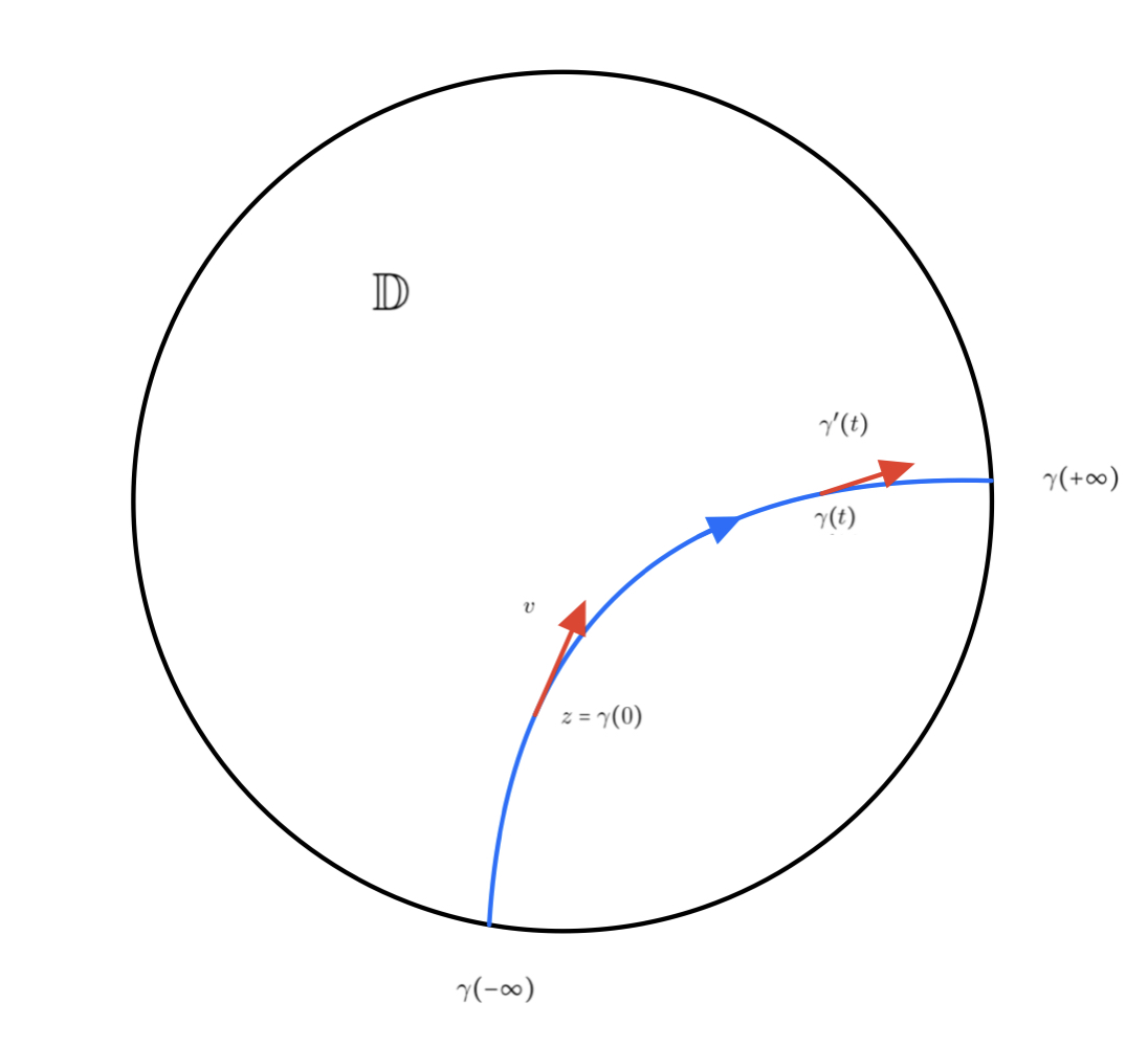
The geodesic flow on the quotient of by a Fuchsian group is defined in the natural way via the projection map . Thus, to link the continuous time geodesic flow with the discrete interval maps, various reductions are required. This is done by choosing a suitable cross section and the corresponding cross section map. A cross section is roughly considered as a subset of which intersects the geodesic flow repeatedly in past and future. There are usually multiple choices available for the cross section.
In our problem we choose the cross section explicitly to be or under the projection map, simply . Intuitively, the part of the billiard trajectory between two consecutive hits is rendered irrelevant. We lift the billiard trajectories to the corresponding pointed geodesics on route to establishing conjucacy between the corresponding space of pointed geodesics and the associated space of codes.
On the contrary in [2], the authors choose a cross section for which a second reduction is possible, which is given by a one-dimensional factor map. Through these two reductions, the relationship between the geodesic flows and interval maps is further discussed. They then relate these interval maps with symbolic systems via the Markov partitions. This line of separation between the two is crucial as we are able to discuss the case of billiards even when a vertex of polygon goes to whereas in [2] the inherent restriction of being compact is maintained throughout. The existence of the fundamental region is essentially based on this. Our model is fairly simple.
The underlying constructions are different in nature and this results in a difference in the nature of the associated symbolic sequences that they obtain in [2] from what we obtain here.
Our results here motivate us to look into the larger picture of shift dynamics. We study the space of all closed shift invariant sets of bi-infinite sequences on finite symbols, given the Hausdorff topology. We particularly demonstrate that ‘shifts of finite type (SFTs)’ form a dense subset of such a space. This gives us convergence in subshifts and we further study the dynamical properties induced by such a convergence.
In Section 2. we discuss some basic theory thus introducing our definitions and notations. We study our billiard dynamics and derive the associated symbolic dynamics and their properties in Section 3. In Section 4, we study convergence of the dynamics in subshifts and polygonal billiards.
2 Preliminaries
In this section, we lay down some basic notions for later usage, thus establishing the notation we will henceforth use.
2.1 Some Topological Dynamics
A discrete dynamical system consists of a continuous self-map on a metric space .
The orbit of a point is the set . Here stands for the fold self-composition of . We note that orbits are invariant sets i.e. for all . The basic study in dynamics is to study the asymptotic behaviour of orbits of all .
The point is periodic if there exists such that . The orbit of a periodic point, which is a finite set, is called a periodic orbit. The set of periodic points of in is denoted by . The set of all limit points of is called the omega-limit set of at , and written as . Omega-limit sets are closed invariant sets. An element is called a recurrent point for if for some , , i.e. . The set of recurrent points of in is denoted by . An element is called a nonwandering point for if for every open , such that . The set of all nonwandering points of is denoted by . The system is said to be non wandering if .
The system is said to be point transitive if there is an such that . These points with dense orbits are called transitive points.
The system is called topologically transitive when for every pair of nonempty, open sets , there exists such that . Notice that is surjective, and so a nonempty, open implies is nonempty and open for every .
These definitions of point transitivity and topological transitivity are equivalent on all perfect, compact metric spaces.
Many times we represent these systems as or where . Such systems are then termed pointed systems or ambits.
The system is minimal when every orbit is dense.
is called topologically mixing if for every pair of nonempty open sets in , there is a such that is nonempty for all .
For , let be the hitting time set. We say that
- •
is transitive if for every pair of nonempty open sets , is nonempty.
- •
is mixing if for every pair of nonempty open sets we have that is cofinite.
An equivariant map is a continuous map such that .
In particular, the diagram
commutes.
When is a homeomorphism we call it a conjugacy and say that and are conjugate. When is surjective we call it a factor map and say that is a factor of .
We note that the properties of entropy, transitivity and topologically mixing are preserved on taking factors.
In [27], the concept of entropy has been extended by Hofer to non-compact Hausdorff spaces. According to [27], for a non-compact space and , the topological entropy
where is a compactification of and is the extension of on . We note that with this definition, it has been shown in [27]:
(1) for each positive integer ,
(2) If is , then ,
(3) For non-compact spaces and and systems and , if satisfies then .
It has been seen that pseudo-orbits, or more formally -chains, are important tools for investigating properties of discrete dynamical systems. They usually capture the recurrent and mixing behaviors depicted by the systems, even though they are highly metric dependent properties.
For , an -chain (or - pseudo-orbit) from to is a sequence such that for . The length of the -chain is said to be .
A point is chain recurrent if for every , there is an -chain from to itself. is chain recurrent if every point of is chain recurrent.
is chain transitive if for every and every , there is an -chain from to . is chain mixing if for every and for any , there is an such that for all , there is an -chain from to of length exactly .
Theorem 2.1.
[3] For , is chain transitive for all . Further, if is chain transitive then it can be embedded in a larger system where it is an omega limit set.
Theorem 2.2.
[6] If is chain transitive, then either is chain mixing or factors onto a non-trivial periodic orbit.
2.2 Symbolic Dynamics
Shift spaces are built on a finite set of symbols which we call the alphabet. Elements of are called letters.
We define the full shift as the collection of all bi-infinite sequences or bi-infinite sequences of symbols from . It is denoted by
The product topology on is metrizable and a compatible metric defined on it can be given as:
| (1) |
for any two sequences and .
The on the full shift maps a point to the point whose ith coordinate is
A shift space is a closed, invariant (i.e. ) set .
Observe that for ,
For , (a nonempty) is a word of length , and we write . If the word is a part of the word then we say that is a subword of and we write .
Similarly for any , we write if appears in as a block, i.e. and for , we write the concatenation . The collection of all nonempty words in is .
Let be the language of shift space i.e. the set of all nonempty words appearing in any . Let be the set of blocks that never appear in any . Usually we can write the shift space as for some collection of forbidden blocks over , i.e. . Every shift space can also be defined by its language . Notice that for we have .
For the shift space , the system is called a subshift.
is called a subshift of finite type (SFT) if the list of forbidden words can be taken to be finite. If is the length of the longest forbidden word, then this SFT is an step SFT. Thus an step SFT has the property that if and , then as well.
Every SFT is topologically conjugate to an edge SFT , presented by some square nonnegative matrix . Here is viewed as the adjacency matrix of some directed graph , whose edge set is the alphabet of the SFT. is the space of bi-infinite sequences corresponding to walks through the graph . Here for every , the terminal vertex of equals the initial vertex of . Thus, a SFT can also be denoted as or where is the associated graph and is the transition matrix.
A non-negative matrix is called irreducible if for every there is such that , and is called aperiodic if there is such that , for every .
A subshift is transitive if for every pair of words , there exists a word with . is mixing if there exists an such that such a can be choosen with for all .
A SFT is transitive if and only if the transition matrix is irreducible, and is mixing if and only if the transition matrix is aperiodic.
SFTs can also be viewed as vertex shifts, where the vertices are labelled by elements in and a directed edge connects two vertices if the concatenation of the labels of these vertices is a permissible word in the language. The transition matrix here is a Boolean matrix.
Here codes play an important role. The most important codes for us are those that do not change with time i.e. codes which intertwine with the shift . A common example of such codes is the sliding block code which we define as follows: Let X be a shift space over . Let be another alphabet and
be a map called (m+n+1)-block map or simply block map, where is the set of all -blocks in . We define a map
given by where . The map is called the sliding block code with memory m and anticipation n induced by .
Theorem 2.3.
(Curtis-Hedlund-Lyndon) Let and be subshifts over finite alphabets and respectively. A continuous map commutes with the shift (i.e., ) if and only if is a sliding block code.
If a sliding block code is onto, it is called a factor code from X onto Y and Y is called a factor of X. If is one-to-one, then it is called embedding of X into Y. is called a conjugacy from X to Y, if it is invertible. The shift spaces in this case are called and we write X Y. Conjugacies carry periodic points to periodic points and in general preserve the dynamical structure.
The topological entropy of a subshift is given as
where denotes the number of words in of length . It is known that the topological entropy of an irreducible SFT equals where is the Perron eigenvalue of .
We refer to [32] for more details.
There is an interesting illustration of Theorem 2.1 for SFTs.
Theorem 2.4.
[8] Let be an invariant and closed subset. Then there is a point such that if and only if is chain transitive.
Remark 2.1.
One of the consequences of the above observation, also observed independently in [35] is - in the case of SFTs, chain transitivity is equivalent to transitivity.
Lastly, we recall some characterization of the language of a subshift from [4] and build on it. We skip the trivial proofs since the arguments are similar to the ones given in [4]. Recall that as varies over , the cylinder sets
comprise a bases of clopen sets on .
- (a)
is transitive(irreducible) if and only if for all and all , there exists such that .
- (b)
is minimal if and only if whenever then for all .
- (c)
is mixing if and only if whenever there exists such that for all there exists with such that .
- (d)
is non wandering if and only if for all there exists , such that .
- (e)
is chain recurrent if and only if for all , there exists and with , such that .
- (f)
is chain transitive if and only if for all and all , there exists and with , such that .
- (g)
is chain mixing if and only if for all and all , there exists such that for all there exists for and with , such that .
2.3 Some Rudiments in Metric Spaces
For a metric space , we denote as the space of all nonempty closed subsets of , and the space of all compact subsets of , endowed with the Hausdorff topology. We note that usually but for compact , .
This has a natural induced metric.
Given a point and a closed set , recall
On we define the Hausdorff metric: For
| (2) |
We note that is a psuedo-metric on and a metric on .
For , let be the neighbourhood of . Thus, if and only if each set is in the open neighborhood of the other i.e. and , or, equivalently, each point of is within of a point in and vice-versa.
When is compact, we occasionally use an equivalent topology on . Define for any collection of open and nonempty subsets of ,
| (3) |
The topology on , generated by such collection as basis, is known as the Vietoris topology.
If is a sequence of closed sets in a then
We recall,
Lemma 2.1.
For a metric space , and a sequence in ,
(a) If converges to in then is compact.
(b) If is compact and is Cauchy then converges to .
(c) If is complete then is complete.
(d) If is compact then is compact.
(e) If is separable then so is .
(f) If is given by , then is an isometric inclusion.
(g) For a continuous map of metric spaces, there is induced the map defined by . If is uniformly continuous or continuous, then the map is also uniformly continuous or continuous, respectively.
(h) The set of all finite subsets of is dense in .
These results also hold when is given the Vietoris topology.
The Gromov-Hausdorff metric furthers the idea of the Hausdorff metric. Given two compact metric spaces and , we define
| (4) |
where denote an isometric embedding of into some metric space and the infimum is taken over all such possible embeddings.
Lemma 2.2.
[18] The following hold with respect to the Gromov-Hausdorff metric:
- 1.
If are compact metric spaces, the .
- 2.
If are not compact then it is possible that , without being isometric. For example .
- 3.
Metric spaces if and only if for every , there exists such that every net in is a limit of nets in .
- 4.
Compact and are isometric if and only if .
We denote the set of all isometric compact metric spaces endowed with the Gromov-Hausdorff metric as . Then the following is known about the metric space .
- 1.
is separable and complete.
- 2.
is not locally compact or compact.
- 3.
The set of all finite metric spaces is dense in .
Such a is called a universal metric space.
2.4 Geodesics and Polygons in the Hyperbolic Plane
A hyperbolic space is a space that has a constant negative sectional curvature. We work in dimension and call it a hyperbolic 2-space or a hyperbolic plane. We will use two models of hyperbolic plane, namely, the Poincaré half plane model which we denote as and the Poincaré disc model denoted as . Both of them model the same geometry in the sense that they can be related by an isometric transformation that preserves all the geometrical properties. We refer to [7, 9, 10] for more details.
The underlying space of the Poincaré half plane model is the upper half-plane in the complex plane , defined to be
We use the usual notion of point and angle that inherits from . The metric on is defined by
The Poincaré disk model is described by
The metric on is defined by
Once we have the notion of distance on a space, we define the respective straight lines as geodesics. They are the locally distance minimising curves of the space. Under the metric imposed on , we get the geodesics to be the euclidean lines perpendicular to real axis and the euclidean semicircles which are orthogonal to the real axis. We note that the real axis along with the point at infinity gives the boundary of . In case of with the above defined metric, we get the geodesics to be the euclidean lines passing through the centre of the disc and the euclidean circles orthogonal to , the boundary of .
A subset of the hyperbolic plane is convex if for each pair of distinct points and in , the closed line segment joining to is contained in . Hyperbolic lines, hyperbolic rays, and hyperbolic segments are convex. Given a hyperbolic line , the complement of in the hyperbolic plane has two components, which are the two open half-planes determined by l. A closed half-plane determined by l is the union of with one of the two open half-planes determined by . We refer to as the bounding line for the half-planes it determines. Open half-planes and closed half-planes in are convex.
Let be a collection of half-planes in the hyperbolic plane, and for each , let be the bounding line for . The collection is called locally finite if for each point in the hyperbolic plane, there exists some so that only finitely many bounding lines of the half-planes in intersect the open hyperbolic disc where
A hyperbolic polygon is a closed convex set in the hyperbolic plane that can be expressed as the intersection of a locally finite collection of closed half-planes. Under this definition, there are some subsets of the hyperbolic plane that satisfy this criteria, but we do not want them to be considered as hyperbolic polygons. For example, a hyperbolic line is a hyperbolic polygon, because it is a closed convex set in the hyperbolic plane that can be expressed as the intersection of the two closed half-planes determined by . A hyperbolic polygon is nondegenerate if it has nonempty interior else it is called degenerate. We will work only with nondegenerate polygons here.
Let be a hyperbolic polygon and let be a hyperbolic line so that intersects and so that is contained in a closed half-plane determined by . If the intersection is a point, we say that this point is a vertex of . The other possibilities are that the intersection is either a closed hyperbolic line segment, a closed hyperbolic ray, or all of . We call this intersection side of . Let be a hyperbolic polygon, and let be a vertex of that is the intersection of two sides and of . Let be the hyperbolic line containing . The union divides the hyperbolic plane into four components, one of which contains . The interior angle of at is the angle between and , measured in the component of the complement of containing . A hyperbolic polygon in the hyperbolic plane has an ideal vertex at if there are two adjacent sides of that are either closed hyperbolic rays or hyperbolic lines that share as an endpoint at infinity.
A finite-sided polygon in the hyperbolic plane is called reasonable if does not contain an open half-plane. A hyperbolic n-gon is a reasonable hyperbolic polygon with sides. A compact polygon is a hyperbolic polygon whose all vertices are in the hyperbolic plane. A compact hyperbolic n-gon is regular if its sides have equal length and if its interior angles are equal. For each , an ideal n-gon is a reasonable hyperbolic polygon that has sides and vertices. Thus, an ideal polygon is a hyperbolic polygon whose all vertices are ideal points (i.e. lying on the boundary of the hyperbolic plane). The hyperbolic polygons with vertices lying both inside the hyperbolic plane and on its boundary are called semi-ideal polygons. An angle at a vertex of a polygon in is called rational if it is of the form where and . The corresponding vertex is called a rational vertex. Thus, a compact polygon is labeled rational if all its vertices are rational and a semi-ideal polygon is called rational if all its non-zero vertex angles are rational. We note that the angle at vertices that are ideal points is zero and so by definition ideal polygons are vacuous rational polygons.
An ideal polygon has infinite perimeter and finite area from Gauss-Bonnet formula. In particular, an ideal -sided polygon has an area and thus is the largest possible polygon in hyperbolic plane. The compact polygons have finite perimeter and area strictly less than . The semi-ideal ones have infinite perimeter and area less than or equal to . The polygons in the hyperbolic plane enjoy a very special feature, namely, the similar polygons are congruent. In particular, all ideal n-gons are congruent to each other. This feature allows us to work in a simplified situation of a symmetrically placed n-gon.
2.5 Tessellating the Hyperbolic Plane and the Katok-Zemlyakov unfolding method
We can consider any one of as the model for the hyperbolic plane. A tessellation of is a subdivision of into polygonal tiles satisfying the following conditions:
(1) such that ,
(2) is either empty, or a single vertex common to both, or an entire common edge,
(3) an isometry of hyperbolic plane such that .
Informally speaking, a collection of tiles tessellate the hyperbolic plane if they cover the plane, don’t overlap, and are of same shape and size.
Let be an ideal polygon in the hyperbolic plane. Then, we can reflect it across each one of its sides and the same procedure can be applied to the reflections and so on. The collection of all such ideal polygons obtained, along with gives us a tessellation of . The figure below shows one such example, where we start with an ideal triangle . Its sides are labeled as in counter-clockwise sense. On reflection about a side , the labels change to . This labelling proceeds in same way for further reflections. Similar tessellation can be obtained for the rational compact polygons and for the semi-ideal polygons with the vertex angles either or rational.
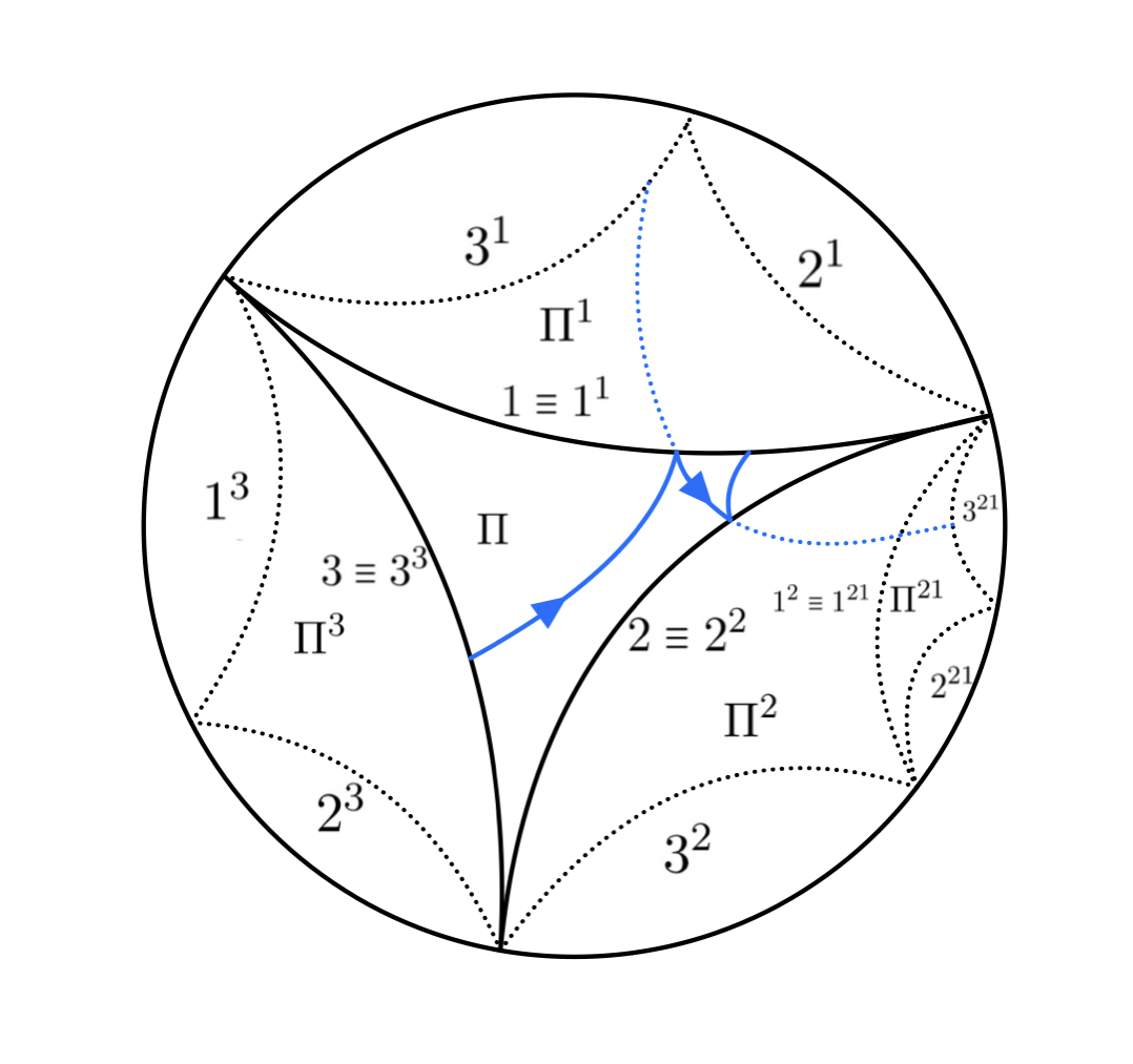
The unfolding technique that we discuss ahead was formally introduced to the domain of billiard dynamics by A.B.Katok and A.N.Zemlyakov [29]. This method converts a polygon on a plane into a surface on which the billiard trajectories appear as geodesics. Under this technique a billiard trajectory in a polygon can be unfolded in an intuitive procedure as follows: Instead of reflecting the trajectory in a side of , we reflect itself in that side which gives a copy of the reflected ray in the new polygon. The join of this new directed line segment with the incident ray in lies on a line. We say that the billiard trajectory has been unfolded at this hit point. When we apply this procedure to the whole billiard trajectory, it gives us straightened version of the billiard trajectory, which we call as unfolded billiard trajectory.
More details on tessellations of polygons in the hyperbolic plane can be found in the elaborated work of S.Katok in [30], wherein it has been described via the Fuchsian groups and the fundamental regions. The tessellations are described via the action of a discrete and properly discontinuous group on a fundamental region. Here, we avoid this nomenclature as our primary object of concern is the polygon (which is already fixed to start with) and the billiard dynamics happening on it.
2.6 Billiards in the Hyperbolic Plane
We consider the Poincaré disc model of the hyperbolic plane.
We carry out our investigations with a class of hyperbolic polygons which we call as ideal polygons, compact rational polygons and semi-ideal rational polygons. The ideal polygons are the ones with all the vertices on and the compact rational polygons are the ones for which all the vertices lie in and have angles that divide into integer parts. The polygons that lie in ‘semi-ideal rational’ class are the ones for which either the vertices lie on or the vertex angles divide into integer parts.
We follow the general construction as defined in [15] for the ideal polygons and in [16] for compact rational polygons.
Let be a k-sided polygon in . A billiard trajectory in the polygon is a directed geodesic flow between each pair of consecutive specular bounces of the boundary(not containing the vertices) of . We have a simple choice for the coordinate system for the directed geodesic arcs. We parameterize the boundary of the Poincaré disc using the azimuthal angle by considering it as a subset of . Thus, we can represent a directed geodesic by the pair , where are the intercepts made by a directed geodesic on with the direction being from to . In this setting we have a natural metric on given by
| (5) |
A billiard trajectory is a curve that is parameterized by the arc-length and consists of the geodesic arcs which are reflected by the walls of the polygon . Therefore, a trajectory can be expressed as
where
We do not consider billiard trajectories starting or ending in vertices of .
The billiard trajectories here follow the grammar rules defined and discussed by Marie-Joya Giannoni, Dennis Ullmo in [15, 16]. Based on that Simon Castle, Norbert Peyerimhoff, Karl Friedrich Siburg [13] prove the rules for ideal polygons.
Theorem 2.5.
[13] Let be an ideal polygon with counter-clockwise enumeration . An equivalence class denoted with is in if and only if
(1) does not contain immediate repetitions, i.e., and
(2) does not contain an infinitely repeated sequence of labels of two adjacent sides.
Moreover, every equivalence class of pointed billiard sequences corresponds to one and only one billiard trajectory.
3 Pointed Geodesics and Billiards in Hyperbolic Polygons
3.1 Pointed Geodesics and Billiards
Definition 3.1.
Let be a billiard trajectory in a polygon in . For a fixed , we will call as a base arc of the trajectory .
We note that base arcs are compact subsets of .
A base arc uniquely determines the billiard trajectory under the restrictions imposed by the specular reflection rule.
Definition 3.2.
For the base arc defining , we call a pointed geodesic.
Thus a pointed geodesic is identified with the element
by clearly establishing the position of the base arc . A natural way of encoding a pointed geodesic is to seize the order in which it hits the sides of , starting from the side hit by the base arc and then reading the past and future hits of the trajectory and pointing out the symbol corresponding to the base arc. If we label the sides of anti-clockwise from 1 to k, then every pointed geodesic produces a bi-infinite sequence with .
Definition 3.3.
Define
as the space of all pointed geodesics on .
and so can be equipped with the natural Hausdorff metric , and so is endowed with the Hausdorff topology.
Here, is simply written as .
We define a function as follows:
| (6) |
where is as in Equation (5).
Proposition 3.1.
Let be the space of pointed geodesics on a polygon in , then defines a metric on .
Proof.
Clearly, is non-negative. If then Therefore, implying . If base arcs of two pointed geodesics are same then the corresponding trajectories are also same because of the dynamics provided by the bounce map. Therefore,
The symmetry and triangle inequality for follows from the respective properties of (the boundary of the Poincaré disc). Therefore, is a metric on .∎
We show that the Hausdorff topology on is same as the topology on given by . Recall that on can be given as follows:
| (7) |
Note that the above definition works because is uniquely determined by a base arc and if then . Thus, this notion of distance between two pointed geodesics is just the Hausdorff distance between the corresponding base arcs. We denote the space of all base arcs on a polygon that are associated with billiard trajectories by or simply , when the context is clear. Note that and is a bounded subset of . Thus, in this case, the Vietoris topology and Hausdorff topology are equivalent on . We, thereby get a natural isometry between and for a polygon , giving a one-to-one correspondence between the Vietoris topology on and the topology generated by on . Under the same pretence, we also have the metric on and the natural isometry between and .
Theorem 3.1.
Let be the space of pointed geodesics on a polygon in , then and generate the same topology on .
Proof.
With the above discussion, it is sufficient to prove that and generate the same topology on . The topology on given by the metric is the induced topology on . For , consider
Therefore,
Without any loss of generality, we assume that is small enough such that the -tube of the base arcs about doesn’t contain any vertex of . The adjoining figure elaborates the schematics. Consider the open balls in such that
and each lying inside the -tube. Since is open in , therefore is open in and is lying in the -tube. Therefore, we have
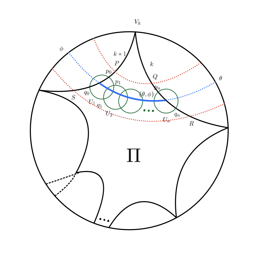
Conversely, consider a basic open set containing a base arc . Without the loss of generality, we assume that are open discs in . Define Note that each is either or contains two points. Define Here, denotes the side of the polygon with label . Define and choose Then, the -tube lies inside .
∎
3.2 Ideal Polygons
3.2.1 Symbolic Dynamics for Billiards in Ideal Polygons
Theorem 2.5 ensures that the set is not dependent on the choice of the ideal polygon . The elements of are restricted only by the rules (1) and (2) defined there.
Let be an ideal polygon that is symmetrically placed on , and let be the space of pointed geodesics on .
Define a map with its action on described as follows :
We will study the dynamics of under the metric .
Theorem 3.2.
Let and be the space of pointed geodesics on . Suppose be the space of all pointed bi-infinite sequences satisfying the rules:
(1) and
(2) does not contain an infinitely repeated sequence or bi-infinite sequence of labels of two adjacent sides.
Then .
Proof.
Define by
Now
.
From [13] , we see that and . This gives the injectivity of h.
The surjectivity of is established from the fact that each defines a unique billiard trajectory . Therefore with corresponding , we get a unique base symbol , which further picks a base arc on , thereby giving us a unique pointed geodesic in i.e.
Thus
.
Therefore, , implying that is a homomorphism.
Consider an open set
in . Thus if and only if Tesselate with and its copies generated by reflecting about its sides and doing the same for the reflected copies along the unfolded geodesic generated by . Let us label the vertices of in anticlockwise sense by and the vertices of the copy of by . Define p to be the largest positive integer such that
Then Therefore, is continuous.

Consider an open set
in . Pick an arbitrary bi-infinite sequence U. Then from corresponding , we get a billiard trajectory using 2.5. By pointing out the base arc corresponding to symbol , we get a pointed geodesic whose billiard bi-infinite sequence, we label as . Now, in general may not be in , but since and belong to same equivalence class, there exists an such that equals . Therefore, has its associated pointed billiard bi-infinite sequence
We construct m future and m past copies of in by reflecting about its sides as suggested by
Label as .
Let be defined as follows :
Choose such that . If then
Thus , i.e. Therefore, is continuous. ∎
Thus, the space of all bi-infinite sequences on a k-sided ideal polygon is given by
Therefore, is not closed as the limit points of of type , , do not lie in . Thus, we further look for the closure of in and define where is the set of all limit points of . Hence,
and thereby is an SFT with forbidden set . Thus, is a dense subset of an SFT. We notice that is a completion of , therefore it is also a compactification of .
Thus, here we obtain a pair of conjugacies between and given by such that and between and with defined as above.
In particular, the diagram
commutes.
3.2.2 Dynamical Properties of Billiards in Ideal Polygons
For an ideal polygon with vertices, the closure of the space of pointed bi-infinite sequences has forbidden set
Thus, the adjacency matrix for the corresponding vertex shift is
Its eigenvalues turn out to be and further combinatorial computations yield
This implies that
Since is a dense subset of , they share the same entropy [27].
We also note that the matrix is aperiodic and so is mixing. Since every element of consists as subword the infinite strings of the form for , we note that is also mixing.
Thus is a mixing system with topological entropy , with being the number of ideal vertices of the polygon .
3.3 Compact Rational Polygons
Now, we consider the case when the vertices of lie inside . The coding for most bounded systems is non-exact and so is the case here for the compact polygons except for the ones that tile . Therefore, to ensure that the fundamental domain tesselates the disc, we only consider the polygons with rational angles. Recall that, an angle at a vertex of a polygon in is called rational if it is of the form where and . We will call the corresponding vertex a rational vertex.
3.3.1 Symbolic Dynamics for Billiards in Compact Rational Polygons
First, we will establish the coding rules for such rational polygons motivated by the discussion in [16]. Theorem 3.3 has been originally discussed in [16]. Here, we present an alternative approach and proof for the same using the basic techniques of topological dynamical systems. We follow this by establishing the conjugacy between the space of corresponding pointed geodesics and the symbolic space defined under the coding rules presented in Theorem 3.3.
Theorem 3.3.
Let be a compact rational polygon with anti-clockwise enumeration of sides labeled . Label the vertices of as with being the respective
interior angles such that the adjacent sides of are and . Further, assume that for each .
Then an equivalence class of bi-infinite sequences, with is in (the space of all equivalence classes of bi-infinite sequences of ) if and only if
(1) does not contain any immediate repetitions of symbols i.e., .
(2) does not contain more than repetitions of two successive symbols and for every .
Moreover, every equivalence class of such bi-infinite sequences corresponds to one and only one billiard trajectory.
Proof.
First, we will establish the necessity of (1) and (2). Consider a bi-infinite sequence attached to a billiard trajectory. In , two distinct geodesics can have at most one intersection, therefore (1) holds. Now, suppose (2) does not hold for i.e., there exists a subword of with repetitions of letters and . Without any loss of generality, let us assume that starts with . Then, on unfolding the corresponding part of the trajectory times, we get the condition at the vertex , which gives a contradiction.
Now, suppose be a bi-infinite sequence for which (1) and (2) hold. We will construct a unique billiard trajectory defined by it in . We split our proof into three parts. First we will prove that if we consider a bi-sequence satisfying (1) and (2) which is periodic, it uniquely defines a billiard trajectory. Then, we will show that the set of periodic bi-infinite sequences satisfying (1) and (2) is dense in the set of all bi-infinite sequences satisfying (1) and (2). Lastly, this will allow us to construct a unique billiard trajectory against an arbitrary bi-infinite sequence satisfying (1) and (2) as the limit of a sequence comprising of periodic bi-infinite sequences satisfying (1) and (2).
The set of all periodic bi-infinite sequences is dense in a full -shift. If we remove bi-infinite sequences containing words and where , and the ones for which for any , the set of all periodic bi-infinite sequences in the remaining space is still dense. Indeed, if we start with satisfying (1) and (2), we can define a sequence of periodic points as follows: take
and so on. An issue with a typical term of such a sequence can be that the maximal repeating word may have starting and ending letters same or adjacent which violates (1) and (2) respectively. As a remedy to this, whenever such a violation happens, we drop that term from the sequence. This procedure still leaves a subsequence (because of the fact that itself satisfies (2) which comprises of periodic points and converges to . Thus, we have the required denseness property.
Suppose is an arbitrary bi-infinite sequence obeying (1) and (2). Let be a sequence generated by the above construction, then . Now, each has a unique geodesic associated with it. Since, is geodesically complete, the sequence of geodesics, converges to a limit geodesic , which acts as the unique geodesic associated with . On folding back into the fundamental polygon , we get a unique billiard trajectory associated with . ∎
Theorem 3.4.
Let be a compact rational polygon with anti-clockwise enumeration of sides labeled . Label the vertices of as ,…, with ,…, being the respective interior angles such that the adjacent sides of are and . Further, assume that for each . Let be the space of pointed geodesics on and the space of all bi-infinite sequences satisfying (1) and (2) from Theorem 3.3. Then .
Proof.
Define by
Now
. From Theorem 3.3 , we see that
This gives the injectivity of h.
The surjectivity of is established from the fact that each defines a unique billiard trajectory as shown in Theorem 3.3.
Therefore with corresponding , we get a unique base symbol , which further picks a base arc on , thereby giving us a unique pointed geodesic in i.e. .
The homomorphism of follows under the same arguments as in Theorem 3.2.
Consider an open set in . Thus if and only if
Since the vertices are rational, it allows us to tesselate with and its copies generated by reflecting about its sides and doing the same for the reflected copies along the unfolded geodesic generated by . Let us label the vertices of in anticlockwise sense by and the vertices of copy of by . We note here that as we replicate along the unfolded geodesic , it shrinks to a point both in future and past in euclidean sense. Define p to be the largest positive integer such that
Then Therefore, is continuous.
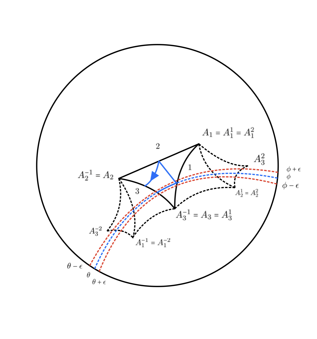
Consider an open set in . Pick an arbitrary bi-infinite sequence U. Then from corresponding , we get a billiard trajectory using Theorem 3.3. By pointing out the base arc corresponding to symbol , we get a pointed geodesic that corresponds to a bi-infinite sequence which we label as . Now, in general may not be in , but since and belong to same equivalence class, there exists an such that equals . Therefore, has its associated billiard bi-infinite sequence
We construct future and past copies of in by reflecting about its sides as suggested by . Label as .
Let be defined as follows :
Choose such that . If , then
Thus , i.e. Therefore, is continuous.
Thus, . ∎
Remark 3.1.
We note that both and generate the same language. gives the trajectories whereas gives each point in the trajectory.
3.3.2 Dynamical Properties of Billiards in Compact Rational Polygons
For a compact polygon with vertices, the space of pointed bi-infinite sequences has forbidden set
Example 3.1.
We consider a particular case here where we consider a compact triangle with . Here, we can declare to be a with
Since is a , we go for .
Note that the associated transition matrix here is aperiodic, and so is mixing. Also this has a positive Perron eigenvalue which gives a positive topological entropy for .
Thus here is a mixing system with positive topological entropy.
In general both and will be mixing systems, that has been proved later in Theorem 3.7. And so will have positive topological entropy.
3.4 Semi-Ideal Rational Polygons
After establishing the codes for the billiards on ideal and compact rational polygons, we now do the same for the case where some vertices of the polygon sit on and some in such that these polygons also tile . We call such polygons semi-ideal rational. The coding rules for the billiards on such polygons is the natural amalgamation of the rules from the ideal and the compact rational polygon case.
Theorem 3.5.
Let be a semi-ideal rational polygon with anti-clockwise enumeration of sides labeled . Label the vertices of as ,…, with ,…, being the respective interior angles such that the adjacent sides of are and . Further, assume that and with . Then an equivalence class with is in (the space of all equivalence classes of pointed billiard bi-infinite sequences of ) if and only if
(1) does not contain any immediate repetitions of symbols i.e., .
(2) does not contain more than repetitions of two successive symbols and for every .
(3) does not contain an infinitely repeated sequence or bi-sequence of labels of two adjacent sides and .
Moreover, every equivalence class of such billiard induced bi-infinite sequences corresponds to one and only one billiard trajectory.
Proof.
Working on the similar lines, as for the case of ideal and compact case, we will start with establishing the necessity of (1), (2) and (3). Consider a bi-infinite sequence attached to a billiard trajectory. Since, two geodesics in a hyperbolic plane can have at most one intersection, therefore (1) holds. Now, suppose (2) does not hold for with
This means that for some , there exists a subword of with repetitions of letters and . Following the same line of argument as in Theorem 3.3, we get a contradiction. Suppose (3) does not hold for with
This means that for some , it contains an infinitely repeated sequence or bi-sequence of labels of sides and . Under Cayley transformation, we can shift the whole billiard table to and an appropriate isometry of allows us to assume that the two sides and are represented on by the vertical lines and . Now, our trajectory hits these two sides repeatedly infinite number of times. if we unfold this part of the trajectory in , the unfolded part of the trajectory being a geodesic lies on a semi-circle centered at real axis. Since a semi-circle can intersect only finitely many lines from the family , therefore we get a contradiction to our assumption that the trajectory has infinitely many parts consisting of consecutive hits on sides and . Thus, the necessity of conditions (1), (2) and (3) is established. Now suppose be a bi-infinite sequence for which (1), (2) and (3) hold. We will construct a unique billiard trajectory defined by it in . We structure the rest of the proof on the similar lines as in Theorem 3.3, going through the three main stages. First, we will prove that if we consider a bi-infinite sequence satisfying (1), (2) and (3) which is periodic, it uniquely defines a billiard trajectory. Then, we will show that the set of periodic bi-infinite sequences satisfying (1), (2) and (3) is dense in the set of all bi-infinite sequences satisfying (1), (2) and (3). Lastly, this will allow us to construct a unique billiard trajectory against an arbitrary bi-infinite sequence satisfying (1), (2) and (3) as the limit of a sequence comprising of periodic bi-infinite sequences satisfying (1), (2) and (3).
The set of all periodic bi-infinite sequences is dense in a full k-shift. If we remove bi-infinite sequences containing words and where for some , or containing an infinitely repeated sequence or bi-infinite sequence of labels of two adjacent sides and for some , or the ones for which for any , the set of all periodic bi-infinite sequences in the remaining space is still dense. Indeed, if we start with satisfying (1), (2) and (3), we can define a sequence of periodic points as follows: take
and so on. An issue with a typical term of such a sequence can be that the maximal repeating word may have starting and ending letters same or adjacent which violates (1), (2) and (3) respectively. As a remedy to this, whenever such a violation happens, we drop that term from the sequence. This procedure still leaves a subsequence (because of the fact that itself satisfies (2) and (3) which comprises of periodic points and converges to . Thus, we have the required denseness property.
Suppose is an arbitrary bi-infinite sequence obeying (1), (2) and (3). Let be a sequence generated by the above construction, then . Now, each has a unique geodesic associated with it. Since, is geodesically complete, the sequence of geodesics, converges to a limit geodesic , which acts as the unique geodesic associated with . On folding back into the fundamental polygon , we get a unique billiard trajectory associated with . ∎
Theorem 3.6.
Let be a semi-ideal rational polygon with anti-clockwise enumeration of sides labeled . Label the vertices of as ,…, with ,…, being the respective interior angles such that the adjacent sides of are and . Further, assume that and with . Let be the space of pointed geodesics on and the corresponding space of all bi-infinite sequences satisfying (1), (2) and (3) from Theorem 3.5. Then .
Proof.
Define by
Now
. From Theorem 3.5 , we see that and . This gives the injectivity of h.
The surjectivity of is established from the fact that each defines a unique billiard trajectory as shown in Theorem 3.5. Therefore with corresponding , we get a unique base symbol , which further picks a base arc on , thereby giving us a unique pointed geodesic in i.e. .
The homomorphism of follows under the same arguments as in Theorem 3.2.
Consider an open set in . Thus if and only if
Since the vertices are rational or ideal, it allows us to tesselate with and its copies generated by reflecting about its sides and doing the same for the reflected copies along the unfolded geodesic generated by . Let us label the vertices of in anticlockwise sense by and the vertices of copy of by . We note here that as we replicate along the unfolded geodesic , it shrinks to a point both in future and past in euclidean sense. The vertices that lie on stay put, whereas the ones lying in move towards the boundary under both future and past limits. Define p to be the largest positive integer such that
Then Therefore, is continuous.

Consider an open set
in . Pick an arbitrary bi-infinite sequence U. Then from corresponding , we get a billiard trajectory using Theorem 3.5. By pointing out the base arc corresponding to symbol , we get a pointed geodesic corresponding to the bi-infinite sequence which we label as . Now, in general may not be in , but since and belong to same equivalence class, an such that equals . Therefore, has its associated billiard bi-infinite sequence . We construct m future and m past copies of in by reflecting about its sides as suggested by
Label as . Let be defined as follows :
Choose such that . If then .
Thus , i.e. Therefore, is continuous.
Thus . ∎
We note that if is the closure of in , then is an SFT.
3.4.1 Dynamical Properties of Billiards in Semi-Ideal Rational Polygons
We note that in case of rational polygons the SFT is mixing. We present a proof for the semi-ideal case and note that it works the same for the compact case(where ).
Theorem 3.7.
Let be a semi-ideal rational polygon with anti-clockwise enumeration of sides labeled . Label the vertices of as ,…, with ,…, being the respective interior angles such that the adjacent sides of are and . Further, assume that and with . Let be the space of pointed geodesics on and the corresponding space of codes satisfying (1), (2) and (3) from 3.5. Then is mixing.
Proof.
We start with assumption that . For every pair of words , our aim is to declare an such that a can be chosen with for all with . Suppose the word ends in and the word starts with , then we can choose two distict labels distinct from . We construct as , where the blocks are repeated times. Here, can be chosen arbitrarily large but has a natural restriction for adjacent under the coding rules that we have laid down in Theorem 3.6. This establishes the mixing property for any associated with a semi-ideal rational polygon with sides equal or more than .
Next, we consider the case where . Under the same notation as above, suppose all of are distinct. Then, we construct as by choosing distinct from . If two of are equal, say , then we choose and construct as . Similar constructions can be done for is any other similarities occur among as we get more room to wiggle around. This establishes the mixing property for any associated with a semi-ideal rational polygon with sides.
Now, we consider the case . The situations where more than one similarities occur among can be handled in same way as discussed above. If all of are distinct, then we construct as where are chosen respecting the respective coding rules. If exactly two of are equal, say , then we choose and construct . Other cases of similarity among can be handled in the same way. This establishes the mixing property for any associated with a semi-ideal rational polygon with sides.
Lastly, for atleast two of the labels are same. If exactly two are same, say , then we construct as . Similarly, if , then we construct as . If two matchings occur among , say , then we choose and construct as . If more than two matchings occur among , it allows us to choose distinct from as we get more room to wiggle around and similar constructions for follow as discussed above. This establishes the mixing property for any associated with a semi-ideal rational polygon with sides.
∎
Remark 3.2.
Note that this also gives mixing for in the compact rational case. In case of semi-ideal rational polygons, the set consists of strings of the form as described in Theorem 3.5. This implies that is also mixing.
Thus is mixing.
This also gives positive topological entropy for .
4 Convergence in the Space of all Subshifts and Hyperbolic Polygons
4.1 The Space of Subshifts
Let be the set of all shift spaces of bi-infinite sequences defined over a finite alphabet with cardinality at least .
For , let . Define , for each , the space of all bi-infinite sequences taking values in indexed by , endowed with the product topology. Then, for each , is metrizable with the metric defined in Equation (1), and can be taken as a compact metric space. Thus for each , we have subshifts .
Now each , . Any shift space can be considered isometric to a subshift for some . Thus with respect to the Gromov-Hausdorff metric as defined in Equation (4), every subshift in is isometrically imbedded in . Thus can be considered as the universal Urysohn space for all subshifts of bi-infinite sequences over a finite alphabet. Every such shift space is isometric to a compact subset of . Hence we can consider .
Thus each subshift , for , can be considered as a subsystem of . We hence call as the universal shift space, and every subshift from is its subsystem.
Consider the metric space . Thus gives a metric on and we lift that metric on the set of subshifts for . We note that this lift is in the sense of Gromov since we identify isometric shift spaces in with some subset of for some .
Our special emphasis will be on , where is the subclass of all subshifts of finite type in . We see that is a very important subset of .
Lemma 4.1.
For every distinct , .
Proof.
Suppose that there exists no such that . Then for every , there exists a such that . This means that such that . Taking , this means that both have the same words of length , for large . This implies , i.e. we get .∎
Theorem 4.1.
is a dense subset of .
Proof.
Let be a shift space and let be an infinite collection of blocks such that .
We borrow this idea from [32]. The elements of can be arranged lexicographically, and accordingly let .
Define for . Then
Thus, . ∎
We try to understand the space .
Suppose in . Then there exists a sequence such that
We note that the set of finite subsets of is dense in . But all of them are not contained in . We consider such that . Since , and is a homeomorphism, just permutes the elements of . Thus, is just a periodic orbit or a finite union of periodic orbits. Also, this can be considered as a vertex shift over a finite alphabet and so .
Again we note that for every periodic orbit , there exists no other element of that can be contained in for every . Thus each finite element of is isolated.
Let be infinite. Then there is a finite such that . Let be the alphabet set for . Then there exists with for some . Else will be finite.
Define . Then and
Hence .
This gives the complete topological structure of the space . Thus, we can say:
Theorem 4.2.
Every finite element of is isolated and every infinite element is an accumulation point in .
Further, for every infinite there exists a sequence in such that .
4.2 Convergence of Dynamics in Subshifts
Let us look into the statement “ in ”.
Definition 4.1.
We say that the subshift is the limit of subshifts and write in if and only if in .
Remark 4.1.
We note that .
We compare the dynamical properties of the sequence of subshifts in to those of the limit . We look into the dynamical properties of the limit that are inherited by this limiting process.
Remark 4.2.
We note that as mentioned in [32], if then the entropies . By the observation in the previous section, for every , we can choose a sequence in with . Now where is the Perron eigenvalue corresponding to , for every . Thus, each can be considered as a limit of a sequence of the form .
This also implies that for , if with then .
Proposition 4.1.
If for some , then there exists a sequence in with such that .
Proof.
For some define succesively
.
Define , for , where the infinite concatenation of with itself. Since each is finite, it is an SFT.
Now and so . ∎
Remark 4.3.
We note that when is minimal, for some , is obtained as a limit of a sequence of finite SFTs. Now if has no isolated points then is sensitive. Since a finite SFT is always equicontinuous, we note that equicontinuity is not preserved by taking limits. However, recurrence is preserved on taking limits.
We can say more:
Theorem 4.3.
For , if with each being a non-wandering SFT, then is chain recurrent.
Proof.
Since , for given , there exists such that for .
Thus for , there exists such that for , is in neighbourhoods of and .
Thus there exist sequence such that
Since each is non-wandering, for there exists and such that
Choose such that , then there exists and such that
This proves the chain recurrence of .∎
Theorem 4.4.
For , if with each a transitive(irreducible) SFT, then is chain transitive.
Proof.
Since , for given , there exists such that for .
Thus for , there exists such that for , are in neighbourhoods of and and .
Thus there exist sequence such that
Since each is transitive, for every there exists and such that
Choose such that , then there exists and such that
This proves the chain transitivity of .∎
And the discussions in Remark 2.1 gives,
Corollary 4.1.
If with each a transitive(irreducible) SFT and , then is transitive.
Example 4.1.
We note that the limit of transitive SFTs need not be transitive.
We consider SFTs , with alphabet and forbidden words
respectively.
We note that in each , a or must be followed by a block of at least .
Also and where
Each is transitive but is not transitive.
We note that is chain transitive.
Example 4.2.
We note that the limit of transitive SFTs can be transitive even when not SFT.
Let be the even shift with alphabet and forbidden words .
We consider SFTs , with alphabet and forbidden words respectively.
We note that in each , a must be followed by a block of at least .
Also and .
We note that each is transitive and is also transitive.
Theorem 4.5.
For , if with each a mixing SFT, then is chain mixing.
Proof.
Since , for given , there exists such that for .
Thus for , there exists such that for , are in neighbourhoods of and and .
Thus there exist sequence such that
Since each is mixing, for every there exists and for all such that
Choose such that , then there exists , and and for , such that
This proves the chain mixing of .∎
And the discussions in Remark 2.1 gives,
Corollary 4.2.
If with each a mixing SFT and , then is mixing.
Remark 4.4.
We can say something more here. Let and let . For let denote the -balls centered around respectively in .
If is also transitive then we note that the hitting times
where this limit is taken in .
This is simple to observe since for every , and , there exists an for which , and for .
4.3 Convergence of Dynamics for Polygonal Billiards
The results that we have established in Theorems 3.2, 3.4, 3.6 indicate the coming together of geometric and dynamical convergence for the class of semi-ideal rational polygons in a sense that we discuss ahead. We construct a sequence of polygons in the semi-ideal rational class that converges to a polygon in the same class. Then, our results indicate that the corresponding sequence of compactifications of the space of codes must converge to the compactification of the space of codes for .
For a sequence of polygons and a polygon with vertices in , we label the vertices of each by with and the vertices of by with . If for each , then we call it the convergence of a polygonal sequence and denote it as . This convergence is in accordance with the Gromov-Hausdorff metric as given in Equation (4).
We consider the full shift on symbols and denote the space of all compact subsets of by . In view of the above discussion, we talk about the convergence of a sequence of compactifications of the spaces of codes of the corresponding polygonal billiard tables under the ambit of the metric structure provided by . It is to be noted here that for a polygonal billiard table of above mentioned class, the corresponding compactification of the space of codes uniquely determines the space of codes itself. This will allow us to trace back our sequence of polygons starting with the convergence of a sequence of associated compactifications of the space of codes in a sense that we describe ahead.
Theorem 4.6.
Let be a sequence of semi-ideal rational polygons in each having vertices and be another such polygon. Further, suppose be the corresponding space of codes for and the corresponding compactification, for each . Let be the space of codes for with compactification . Then implies .
Proof.
Let then . We note here that for the given counter-clockwise labelling of each , we label as suggested by the above convergence. Consider any arbitrary . If is an ideal vertex, then with , we get for sufficiently large . Now, moving to a subsequence with non-zero terms, if needed, we get for sufficiently large . Note that the zero terms of the sequence, if present satisfy the below mentioned criteria vacuously. Thus, for sufficiently large , we have . Therefore, as contains .
If is a non-zero rational, then for sufficiently large . Say, , then if , we get for sufficiently large . Thus, for sufficiently large , which further implies that for sufficiently large . Therefore, in metric. ∎
Remark 4.5.
We note that we can recover and from and to see that in the sense of Gromov.
Remark 4.6.
The converse of the Theorem 4.6 is more subtle. We describe the case of an ideal triangle . We can assume that is so placed that it contains the center of . This can be done as the coding rules are not dependent on the position of the vertices, thereby the polygon can be tweaked as required. Its corresponding is described by the forbidden set . Let us pick up a sequence given by the corresponding forbidden sets . Then in the metric. For the corresponding is determined by the coding rules of Theorem 3.2. We call the center of as and construct the radial Euclidean lines . Next, we choose a sequence of polygons by taking and placing on . Note that for each the choice of is unique under the requirement that . This ensures that and gives us a partial answer to the converse of Theorem 4.6. The same can be said about an arbitrary ideal polygon. We also remark here that the above construction still holds good for any semi-ideal rational polygon with the restriction that exactly one vertex is in with all other vertices sitting on .
Acknowledgements
We thank Mike Boyle for many helpful discussions on subshifts, and a very generous Anonymous Referee for many useful suggestions improving the readability of this article.
References
- [1] Adam Abrams, Svetlana Katok, Adler and Flatto revisited: cross-sections for geodesic flow on compact surfaces of constant negative curvature, Studia Math., 246 (2019), 167 - 202.
- [2] R.Adler, L.Flatto, Geodesic Flows, Interval maps and Symbolic Dynamics, Bull. Amer. Math. Soc. 25 (1991), 229 -334.
- [3] Ethan Akin, The general topology of dynamical systems, Graduate Studies in Mathematics, vol. 1, American Mathematical Society, Providence, RI, (1993).
- [4] Ethan Akin, Joseph Auslander, Anima Nagar, Variations on the concept of topological transitivity, Studia Mathematica 235 (2016), 225-249.
- [5] Ethan Akin, Joseph Auslander, Anima Nagar, Dynamics of induced systems, Ergodic Theory Dynam. Systems 37 (2017), no. 7, 2034-2059.
- [6] Ethan Akin, Jim Wiseman, Varieties of mixing, Trans. Amer. Math. Soc. 372 (2019), no. 6, 4359-4390.
- [7] James W.Anderson, Hyperbolic Geometry, Springer-Verlag London Limited (2005).
- [8] Andrew Barwell, Chris Good, Robin Knight, Brian E.Raines, A characterization of -limit sets in shift spaces, Ergod. Th. & Dynam. Sys. (2010), 30, 21-31.
- [9] Alan F.Beardon, The Geometry of Discrete Groups, Springer-Verlag New York Inc. (1983).
- [10] Tim Bedford, Michael Keane, Caroline Series, Ergodic theory, Symbolic dynamics and Hyperbolic spaces, Oxford University Press (1991).
- [11] L.Bunimovich, The Ergodic Properties of Certain Billiards(Russian), Funkcional. Anal. i Prilozen, 8, (1974), 73-74.
- [12] Dmitri Burago, Yuri Burago, Sergei Ivanov, A course in metric geometry, Graduate Studies in Mathematics, American Mathematical Society, Providence, RI, (2001).
- [13] Simon Castle, Norbert Peyerimhoff, Karl Friedrich Siburg, Billiards in ideal hyperbolic polygons, Discrete Contin. Dyn. Syst. 29 (2011), no. 3, 893-908.
- [14] Nikolai Chernov, Roberto Markarian, Chaotic Billiards, American Mathematical Society(2006).
- [15] Marie-Joya Giannoni, Dennis Ullmo, Coding Chaotic billiards : I, Physica D: Nonlinear Phenomena, 41 (1990), 371-390.
- [16] Marie-Joya Giannoni, Dennis Ullmo, Coding Chaotic billiards : II, Physica D: Nonlinear Phenomena, Volume 84 (1995), 329-356.
- [17] W.H.Gottschalk and G.A.Hedlund, Topological dynamics, Amer. Math. Soc. Colloquium Publications, vol. 36 (1955).
- [18] Misha Gromov, Metric structures for Riemannian and non-Riemannian spaces. Based on the 1981 French original. Translated from the French by Sean Michael Bates. Progress in Mathematics, 152, Birkhäuser Boston, Inc., Boston, MA (1999).
- [19] Eugene Gutkin, Billiards in Polygons, Physica D, 19 (1986), 311-333.
- [20] Eugene Gutkin and V.Schroeder, Connecting geodesics and security of configurations in compact locally symmetric spaces, Geom. Dedicata 118 (2006), 185 - 208.
- [21] Eugene Gutkin, Geometry, topology and dynamics of geodesic flows on noncompact polygonal surfaces, Regul. Chaotic Dyn. 15 (2010), no. 4-5, 482-503.
- [22] Eugene Gutkin, Billiard Dynamics : An updated survey with the emphasis on open problems, Chaos 22 (2012), no. 2, 116-128.
- [23] M. Gutzwiller, Classical Quantization of a Hamiltonian with Ergodic behavior, Physical Review Letters. 45(3) (1980), 150-153.
- [24] M. Gutzwiller, The Geometry of Quantum Chaos, Physica Scripta T9 (1985), 184-192.
- [25] M. Gutzwiller, Chaos in Classical and Quantum Mechanics, Interdisciplinary Applied Mathematics 1, Springer-Verlag, New York, (1990).
- [26] G.A. Hedlund, The dynamics of geodesic flows, Bull. Amer. Math. Soc., 45 (1939), 241-260.
- [27] J. E. Hofer, Topological Entropy for Non Compact Spaces, Michijan Math. J., 21 (1974), 235-242.
- [28] A. Illanes and S.B. Nadler Jr., Hyperspaces: Fundamentals and Recent Advances (Monographs and Textbooks in Pure and Applied Mathematics, 216), Marcel Dekker, New York (1999).
- [29] A. Katok, A. Zemlyakov, Topological Transitivity of Billiards in Polygons, Math. Notes, 18 (1975), 760-764.
- [30] Svetlana Katok, Fuchsian Groups, The University of Chicago Press (1992).
- [31] Svetlana Katok and Ilie Ugarcovici, Symbolic Dynamics for the Modular surface and beyond, Bull Amer. Math. Soc., 44(2007), 87 -132.
- [32] D. Lind and B. Marcus, An Introduction to Symbolic Dynamics and Coding, Cambridge University Press (1995).
- [33] E. Micheal, Topologies on spaces of subsets, Trans. Amer. Math. Soc. 71 (1951).
- [34] Marston Morse and Gustav Hedlund, Symbolic dynamics, American Journal of Mathematics 60 (1938), 815–866.
- [35] David Richeson, Jim Wiseman, Chain recurrence rates and topological entropy, Topology Appl. 156 (2008), no. 2, 251-261.
- [36] R.E. Schwartz, Obtuse Triangular Billiards I: Near the (2,3,6) triangle, Experimental Mathematics, 15 No. 2 (2006), 161-182.
- [37] R.E. Schwartz, Obtuse Triangular Billiards II: Near the (2,3,6) triangle, Experimental Mathematics, 18 No. 2 (2009), 137-171.
- [38] C.Series, Symbolic dynamics for geodesic flows, Acta Math. 146, (1981), 103-128.
- [39] C.Series, Geometrical Markov coding of geodesics on surfaces of constant negative curvature, Ergodic Theory Dynamical Systems 6, (1986), 601-625.
- [40] Serge Tabachnikov, Geometry and Billiards, American Mathematical Society (2005).
- [41] Loring W. Tu, An Introduction to Manifolds, Springer (2008).
- [42] Jan de Vries, Elements of Topological Dynamics, Mathematics and its Applications 257, Kluwer, Dordrecht, (1993).