跳到论文正文
W Papers独立论文阅读器 arXiv:2002.07839 论文正文 计算阅读时间 · 0%
引用这篇论文根据当前论文元数据生成,正式投稿前建议核对。


License: arXiv.org perpetual non-exclusive license
arXiv:2002.07839v2 [cs.LG] 20 Jul 2020

 
Is Local SGD Better than Minibatch SGD?
 

Blake Woodworth
Toyota Technological Institute at Chicago
blake@ttic.edu
Kumar Kshitij Patel
Toyota Technological Institute at Chicago
kkpatel@ttic.edu
Sebastian U. Stich
EPFL
sebastian.stich@epfl.ch
Zhen Dai
University of Chicago
zhen9@uchicago.edu


Brian Bullins
Toyota Technological Institute at Chicago
bbullins@ttic.edu
H. Brendan McMahan
Google
mcmahan@google.com
Ohad Shamir
Weizmann Institute
of Science
ohad.shamir@weizmann.ac.il
Nathan Srebro
Toyota Technological Institute at Chicago
nati@ttic.edu
Abstract

We study local SGD (also known as parallel SGD and federated averaging), a natural and frequently used stochastic distributed optimization method. Its theoretical foundations are currently lacking and we highlight how all existing error guarantees in the convex setting are dominated by a simple baseline, minibatch SGD. (1) For quadratic objectives we prove that local SGD strictly dominates minibatch SGD and that accelerated local SGD is minimax optimal for quadratics; (2) For general convex objectives we provide the first guarantee that at least sometimes improves over minibatch SGD; (3) We show that indeed local SGD does not dominate minibatch SGD by presenting a lower bound on the performance of local SGD that is worse than the minibatch SGD guarantee.

1 Introduction

It is often important to leverage parallelism in order to tackle large scale stochastic optimization problems. A prime example is the task of minimizing the loss of machine learning models with millions or billions of parameters over enormous training sets.

One popular distributed approach is local stochastic gradient descent (SGD) [36, 1, 35, 23], also known as ‘‘parallel SGD’’ or ‘‘Federated Averaging’’11 1 Federated Averaging is a specialization of local SGD to the federated setting, where (a) data is assumed to be heterogenous (not i.i.d.) across workers, (b) only a handful of clients are used in each round, and (c) updates are combined with a weighted average to accommodate unbalanced datasets. [17], which is commonly applied to large scale convex and non-convex stochastic optimization problems, including in data center and “Federated Learning” settings [11]. Local SGD uses MM parallel workers which, in each of RR rounds, independently execute KK steps of SGD starting from a common iterate, and then communicate and average their iterates to obtain the common iterate from which the next round begins. Overall, each machine computes T=K​RT=KR stochastic gradients and executes K​RKR SGD steps locally, for a total of N=K​R​MN=KRM overall stochastic gradients computed (and so N=K​R​MN=KRM samples used), with RR rounds of communication (every KK steps of computation).

Given the appeal and usage of local SGD, there is significant value in understanding its performance and limitations theoretically, and in comparing it to other alternatives and baselines that have the same computation and communication structure. That is, other methods that are distributed across MM machines and compute KK gradients per round of communication for RR rounds, for a total of T=K​RT=KR gradients per machine and RR communication steps. This structure can also be formalized through the graph oracle model of Woodworth et al. 2018.

So, how does local SGD compare to other algorithms with the same computation and communication structure? Is local SGD (or perhaps an accelerated variant) optimal in the same way that (accelerated) SGD is optimal in the sequential setting? Is it better than baselines?

A natural alternative and baseline is minibatch SGD [3, 2, 20] – a simple method for which we have a complete and tight theoretical understanding. Within the same computation and communication structure, minibatch SGD can be implemented as follows: Each round, calculate the KK stochastic gradient estimates (at the current iterate) on each machine, and then average all K​MKM estimates to obtain a single gradient estimate. That is, we can implement minibatch SGD that takes RR stochastic gradient steps, with each step using a minibatch of size K​MKM—this is the fair and correct minibatch SGD to compare to, and when we refer to “minibatch SGD” we refer to this implementation (RR steps with minibatch size K​MKM).

Local SGD seems intuitively better than minibatch SGD, since even when the workers are not communicating, they are making progress towards the optimum. In particular, local SGD performs KK times more updates over the course of optimization, and can be thought of as computing gradients at less “stale” and more “updated” iterates. For this reason, it has been argued that local SGD is at least as good as minibatch SGD, especially in convex settings where averaging iterates cannot hurt you. But can we capture this advantage theoretically to understand how and when local SGD is better than minibatch SGD? Or even just establish that local SGD is at least as good?

A string of recent papers have attempted to analyze local SGD for convex objectives, [23, 25, 13, 4, e.g.]. However, a satisfying analysis has so far proven elusive. In fact, every analysis that we are aware of for local SGD in the general convex (or strongly convex) case with a typical noise scaling (e.g. as arising from supervised learning) not only does not improve over minibatch SGD, but is actually strictly dominated by minibatch SGD! But is this just a deficiency of these analyses, or is local SGD actually not better, and perhaps worse, than minibatch SGD? In this paper, we show that the answer to this question is “sometimes.” There is a regime in which local SGD indeed matches or improves upon minibatch SGD, but perhaps surprisingly, there is also a regime in which local SGD really is strictly worse than minibatch SGD.

Our contributions

In Section 3, we start with the special case of quadratic objectives and show that, at least in this case, local SGD is strictly better than minibatch SGD in the worst case, and that an accelerated variant is even minimax optimal.

We then turn to general convex objectives. In Section 4 we prove the first error upper bound on the performance of local SGD which is not dominated by minibatch SGD’s upper bound with a typical noise scaling. In doing so, we identify a regime (where MM is large and K≳RK\gtrsim R) in which local SGD performs strictly better than minibatch in the worst case. However, our upper bound does not show that local SGD is always as good or better than minibatch SGD. In Section 5, we show that this is not just a failure of our analysis. We prove a lower bound on the worst-case error of local SGD that is higher than the worst-case error of minibatch SGD in a certain regime! We demonstrate this behaviour empirically, using a logistic regression problem where local SGD indeed behaves much worse than mini-batch SGD in the theoretically-predicted problematic regime.

Thus, while local SGD is frequently better than minibatch SGD—and we can now see this both in theory and in practice [31, 15, 35, see experiments by e.g.]—our work identifies regimes in which users should be wary of using local SGD without considering alternatives like minibatch SGD, and might want to seek alternative methods that combine the best of both, and attain optimal performance in all regimes.

2 Preliminaries

We consider the stochastic convex optimization problem:

minx∈ℝd⁡F⁡(x):=𝔼z∼𝒟​[f⁡(x,z)].\min_{x\in\mathbb{R}^{d}}F(x):=\underset{z\sim\mathcal{D}}{\mathbb{E}}\left[f(x;z)\right]\,. (1)

We will study distributed first-order algorithms that compute stochastic gradient estimates at a point x∈ℝdx\in\mathbb{R}^{d} via ∇f​(x,z)\nabla f(x;z) based on indpendent samples z∼𝒟z\sim\mathcal{D}. Our focus is on objectives FF that are HH-smooth, either (general) convex or λ\lambda-strongly convex22 2 An HH-smooth and λ\lambda-strongly convex function satisfies λ2​‖x−y‖2≤F⁡(y)−F⁡(x)−⟨∇F​(x),y−x⟩≤H2​‖x−y‖2\frac{\lambda}{2}\left\|x-y\right\|^{2}\leq F(y)-F(x)-\left\langle\nabla F(x),y-x\right\rangle\leq\frac{H}{2}\left\|x-y\right\|^{2}. We allow λ=0\lambda=0 in which case FF is general convex., with a minimizer x∗∈arg​minx⁡F​(x)x^{*}\in\argmin_{x}F(x) with ‖x∗‖≤B\|x^{*}\|\leq B. We consider ∇f\nabla f which has uniformly bounded variance, i.e. supx𝔼z∼𝒟​‖∇f​(x,z)−∇F​(x)‖2≤σ2\sup_{x}\mathbb{E}_{z\sim\mathcal{D}}\left\|\nabla f(x;z)-\nabla F(x)\right\|^{2}\leq\sigma^{2}. We use ℱ⁡(H,λ,B,σ2)\mathcal{F}(H,\lambda,B,\sigma^{2}) to refer to the set of all pairs (f,𝒟)(f,\mathcal{D}) which satisfy these properties. All of the analysis in this paper can be done either for general convex or strongly convex functions, and we prove all of our results for both cases. For conciseness and clarity, when discussing the results in the main text, we will focus on the general convex case. However, the picture in the strongly convex case is mostly the same.

An important instance of (1) is a supervised learning problem where f⁡(x,z)=ℓ⁡(⟨x,ϕ⁡(z)⟩,label​(z))f(x;z)=\ell\left(\left\langle x,\phi(z)\right\rangle,\textit{label}(z)\right) is the loss on a single sample. When |ℓ′|,|ℓ′′|≤1\lvert\ell^{\prime}\rvert,\lvert\ell^{\prime\prime}\rvert\leq 1 (referring to derivatives w.r.t. the first argument), then H≤|ℓ′′|​‖ϕ⁡(z)‖2≤‖ϕ⁡(z)‖2H\leq\lvert\ell^{\prime\prime}\rvert\|\phi(z)\|^{2}\leq\|\phi(z)\|^{2} and also σ2≤‖∇f‖2≤|ℓ′|2​‖ϕ⁡(z)‖2≤‖ϕ⁡(z)‖2\sigma^{2}\leq\|\nabla f\|^{2}\leq\lvert\ell^{\prime}\rvert^{2}\|\phi(z)\|^{2}\leq\|\phi(z)\|^{2}. Thus, assuming that the upper bounds on ℓ′,ℓ′′\ell^{\prime},\ell^{\prime\prime} are comparable, the relative scaling of parameters we consider as most “natural” is H≈σ2H\approx\sigma^{2}.

For simplicity, we consider initializing all algorithms at zero. Then, Local SGD with MM machines, KK stochastic gradients per round, and RR rounds of communication calculates its ttth iterate on the mmth machine for t∈[K​R]t\in[KR] via

xtm={xt−1m−η∇f(xt−1m;zt−1m)K|t1M∑m′=1Mxt−1m′−η∇f(xt−1m′;zt−1m′)K|t\hskip-4.2679ptx_{t}^{m}=\begin{cases}x_{t-1}^{m}-\eta\nabla f(x_{t-1}^{m};z_{t-1}^{m})&K\not|\ t\\ \frac{1}{M}\sum_{m^{\prime}=1}^{M}x_{t-1}^{m^{\prime}}-\eta\nabla f(x_{t-1}^{m^{\prime}};z_{t-1}^{m^{\prime}})&K\ |\ t\end{cases} (2)

where ztm∼𝒟z_{t}^{m}\sim\mathcal{D} i.i.d., and K|tK\ |\ t refers to KK dividing tt. For each r∈[R]r\in[R], minibatch SGD calculates its rrth iterate via

xr=xr−1−ηM​K​∑i=1M​K∇f​(xr−1,zr−1i)x_{r}=x_{r-1}-\frac{\eta}{MK}\sum_{i=1}^{MK}\nabla f(x_{r-1};z_{r-1}^{i}) (3)

We also introduce another strawman baseline, which we will refer to as “thumb-twiddling” SGD. In thumb-twiddling SGD, each machine computes just one (rather than KK) stochastic gradients per round of communication and “twiddles its thumbs” for the remaining K−1K-1 computational steps, resulting in RR minibatch SGD steps, but with a minibatch size of only MM (instead of K​MKM, i.e. as if we used K=1K=1). This is a silly algorithm that is clearly strictly worse than minibatch SGD, and we would certainly expect any reasonable algorithm to beat it. But as we shall see, previous work has actually struggled to show that local SGD even matches, let alone beats, thumb-twiddling SGD. In fact, we will show in Section 5 that, in certain regimes, local SGD truly is worse than thumb-twiddling.

For a particular algorithm 𝖠\mathsf{A}, we define its worst-case performance with respect to ℱ⁡(H,λ,B,σ2)\mathcal{F}(H,\lambda,B,\sigma^{2}) as:

ϵ𝖠=max(f,𝒟)∈ℱ⁡(H,λ,B,σ2)⁡F⁡(x^𝖠)−F⁡(x∗)\epsilon_{\mathsf{A}}=\max_{(f,\mathcal{D})\in\mathcal{F}(H,\lambda,B,\sigma^{2})}F(\hat{x}_{\mathsf{A}})-F(x^{*}) (4)

The worst-case performance of minibatch SGD for general convex objectives is tightly understood [18, 3]:

ϵMB-SGD=Θ⁡(H​B2R+σ​BM​K​R).\epsilon_{\textrm{MB-SGD}}=\Theta\left(\frac{HB^{2}}{R}+\frac{\sigma B}{\sqrt{MKR}}\right). (5)

In order to know if an algorithm like local or minibatch SGD is “optimal” in the worst case requires understanding the minimax error, i.e. the best error that any algorithm with the requisite computation and communication structure can guarantee in the worst case. This requires formalizing the set of allowable algorithms. One possible formalization is the graph oracle model of Woodworth et al. 2018 which focuses on the dependence structure between different stochastic gradient computations resulting from the communication pattern. Using this method, Woodworth et al. 2018 prove lower bounds which are applicable to our setting. Minibatch SGD does not match these lower bounds (nor does accelerated minibatch SGD, see Cotter et al. 2011), but these lower bounds are not known to be tight, so the minimax complexity and minimax optimal algorithm are not yet known.

Table 1: Comparison of existing analyses of Local SGD for general convex functions, with constant factors and low-order terms (in the natural scaling H≈σ2H\approx\sigma^{2}) omitted. We applied existing upper bounds as optimistically as possible, e.g. making additional assumptions where necessary to apply the guarantee to our setting, and our derivations are explained in Appendix A. The bolded term is the one which compares least favorably against minibatch SGD. Analogous rates for strongly convex functions are given in Appendix A.
Minibatch SGD H​B2R+σ​BM​K​R\frac{HB^{2}}{R}+\frac{\sigma B}{\sqrt{MKR}}
Thumb-twiddling SGD H​B2R+σ​BM​R\frac{HB^{2}}{R}+\frac{\sigma B}{\sqrt{MR}}
Stich 2018 𝐇𝐁𝟐𝐑𝟐/𝟑+H​B2(K​R)3/5+σ​BM​K​R\mathbf{\frac{HB^{2}}{R^{2/3}}}+\frac{HB^{2}}{(KR)^{3/5}}+\frac{\sigma B}{\sqrt{MKR}}
Stich and Karimireddy 2019 𝐇𝐁𝟐​𝐌𝐑+σ​BM​K​R\mathbf{\frac{HB^{2}M}{R}}+\frac{\sigma B}{\sqrt{MKR}}
Khaled et al. 201933 3 This upper bound applies only when M≤K​RM\leq KR. It also requires smoothness of each f⁡(x,z)f(x;z) individually, i.e. not just FF. σ𝟐​𝐌𝐇𝐑+H2​B2+σ2H​M​K​R\mathbf{\frac{\sigma^{2}M}{HR}}+\frac{H^{2}B^{2}+\sigma^{2}}{H\sqrt{MKR}}
Our upper bound (Section 4) (𝐇​σ𝟐​𝐁𝟒)𝟏/𝟑(𝐊​𝐑)𝟐/𝟑+H​B2K​R+σ​BM​K​R\mathbf{\frac{\left(H\sigma^{2}B^{4}\right)^{1/3}}{(\sqrt{K}R)^{2/3}}}+\frac{HB^{2}}{KR}+\frac{\sigma B}{\sqrt{MKR}}
Our lower bound (Section 5) (𝐇​σ𝟐​𝐁𝟒)𝟏/𝟑(𝐊𝐑)𝟐/𝟑+σ​BM​K​R\mathbf{\frac{\left(H\sigma^{2}B^{4}\right)^{1/3}}{(KR)^{2/3}}}+\frac{\sigma B}{\sqrt{MKR}}
Existing analysis of local SGD

Table 1 summarizes the best existing analyses of local SGD that we are aware of that can be applied to our setting. We present the upper bounds as they would apply in our setting, and after optimizing over the stepsize and other parameters. A detailed derivation of these upper bounds from the explicitly-stated theorems in other papers is provided in Appendix A. As we can see from the table, in the natural scaling H=σ2H=\sigma^{2}, every previous upper bound is strictly dominated by minibatch SGD. Worse, these upper bounds can even be worse than even thumb-twiddling SGD when M≫RM\gg R (although they are sometimes better). In particular, the first term of each previous upper bound (in terms of M,K,RM,K,R) is never better than R−1R^{-1} (the optimization term of minibatch and thumb-twiddling SGD), and can be much worse.

We should note that in an extremely low noise regime σ2≤H2​B2​min⁡{1M,KR}\sigma^{2}\leq H^{2}B^{2}\min\{\frac{1}{M},\frac{K}{R}\}, the bound of Khaled et al. 2019 can sometimes improve over minibatch SGD. However, this only happens when K​RKR steps of sequential SGD is better than minibatch SGD—i.e. when you are better off ignoring M−1M-1 of the machines and just doing serial SGD on a single machine (such an approach would have error H​B2K​R+σ​BK​R\frac{HB^{2}}{KR}+\frac{\sigma B}{\sqrt{KR}}). This is a trivial regime in which every update for any of these algorithms is essentially an exact gradient descent step, thus there is no need for parallelism in the first place. See Appendix A.3 for further details. The upper bound we develop in Section 4, in contrast, dominates their guarantee and shows an improvement over minibatch that cannot be achieved on a single machine (i.e. without leveraging any parallelism). Furthermore, this improvement can occur even in the natural scaling H=σ2H=\sigma^{2} and even when minibatch SGD is better than serial SGD on one machine.

We emphasize that Table 1 lists the guarantees specialized to our setting—some of the bounds are presented under slightly weaker assumptions, or with a more detailed dependence on the noise: Stich and Karimireddy 2019, Haddadpour et al. 2019a analyze local SGD assuming not-quite-convexity; and Wang and Joshi 2018, Dieuleveut and Patel 2019 derive guarantees under both multiplicative and additive bounds on the noise. Dieuleveut and Patel 2019 analyze local SGD with the additional assumption of a bounded third derivative, but even with this assumption do not improve over mini-batch SGD. Numerous works study local SGD in the non-convex setting [35, 30, 27, 25, 9, see e.g.]. Although their bounds would apply in our convex setting, due to the much weaker assumptions they are understandably much worse than minibatch SGD. There is also a large body of work studying the special case R=1R=1, i.e. where the iterates are averaged just one time at the end [36, 32, 14, 19, 7, 10]. However, these analyses do not easily extend to multiple rounds, and the R=1R=1 constraint can provably harm performance [21, see]. Finally, local SGD has been studied with heterogeneous data, i.e. where each machine receives stochastic gradients from different distributions—see Kairouz et al. 2019 a recent survey.

An Alternative Viewpoint: Reducing Communication

In this work, we focus on understanding the best achievable error for a given MM, KK, and RR. However, one might also want to know to what extent it is possible to reduce communication without paying for it. Concretely, fix T=K​RT=KR, and consider as a baseline an algorithm which computes TT stochastic gradients on each machine sequentially, but is allowed to communicate after every step. We can then ask to what extent we can compete against this baseline while using less communication. One way to do this is to use Local SGD, which reduces communcation by a factor of KK. However, the amount by which we can reduce communcation using Local SGD is easily determined once we know the error of Local SGD for each fixed KK. Therefore, this viewpoint of reducing communcation is essentially equivalent to the one we take.

3 Good News: Quadratic Objectives

As we have seen, existing analyses of local SGD are no better than that of minibatch SGD. In the special case where FF is quadratic, we will now show that not only is local SGD sometimes as good as minibatch SGD, but it is always as good as minibatch SGD, and sometimes better. In fact, an accelerated variant of local SGD is minimax optimal for quadratic objectives. More generally, we show that the local SGD anologue for a large family of serial first-order optimization algorithms enjoys an error guarantee which depends only on the product K​RKR and not on KK or RR individually. In particular, we consider the following family of linear update algorithms:

Definition 1 (Linear update algorithm).

We say that a first-order optimization algorithm is a linear update algorithm if, for fixed linear functions ℒ1(t),ℒ2(t)\mathcal{L}^{(t)}_{1},\mathcal{L}^{(t)}_{2}, the algorithm generates its t+1t+1st iterate according to

xt+1=ℒ2(t)​(x1,…,xt,∇f​(ℒ1(t)​(x1,…,xt),zt))x_{t+1}=\mathcal{L}^{(t)}_{2}\left(x_{1},\dots,x_{t},\nabla f\left(\mathcal{L}^{(t)}_{1}\left(x_{1},\dots,x_{t}\right);z_{t}\right)\right) (6)

This family captures many standard first-order methods including SGD, which corresponds to the linear mappings ℒ1(t)​(x1,…,xt)=xt\mathcal{L}^{(t)}_{1}\left(x_{1},\dots,x_{t}\right)=x_{t} and xt+1=xt−ηt∇f(xt;zt)x_{t+1}=x_{t}-\eta_{t}\nabla f(x_{t};z_{t}). Another notable algorithm in this class is AC-SA [6], an accelerated variant of SGD which also has linear updates. Some important non-examples, however, are adaptive gradient methods like AdaGrad [16, 5]—these have linear updates, but the linear functions are data-dependent.

For a linear update algorithm 𝒜\mathcal{A}, we will use local-𝒜\mathcal{A} to denote the local SGD analogue with 𝒜\mathcal{A} replacing SGD. That is, during each round of communication, each machine independently executes KK iterations of 𝒜\mathcal{A} and then the MM resulting iterates are averaged. For quadratic objectives, we show that this approach inherits the guarantee of 𝒜\mathcal{A} with the benefit of variance reduction:

Theorem 1.

Let 𝒜\mathcal{A} be a linear update algorithm which, when executed for TT iterations on any quadratic (f,𝒟)∈ℱ⁡(H,λ,B,σ2)(f,\mathcal{D})\in\mathcal{F}(H,\lambda,B,\sigma^{2}), guarantees 𝔼​F​(xT)−F∗≤ϵ⁡(T,σ2)\mathbb{E}F(x_{T})-F^{*}\leq\epsilon(T,\sigma^{2}). Then, local-𝒜\mathcal{A}’s averaged final iterate x¯K​R=1M​∑m=1MxK​Rm\bar{x}_{KR}=\frac{1}{M}\sum_{m=1}^{M}x_{KR}^{m} will satisfy 𝔼​F​(x¯K​R)−F∗≤ϵ⁡(K​R,σ2M)\mathbb{E}F(\bar{x}_{KR})-F^{*}\leq\epsilon(KR,\frac{\sigma^{2}}{M}).

We prove this in Appendix B by showing that the average iterate x¯t\bar{x}_{t} is updated according to 𝒜\mathcal{A}—even in the middle of rounds of communication when x¯t\bar{x}_{t} is not explicitly computed. In particular, we first show that

x¯t+1=ℒ2(t)​(x¯1,…,x¯t,1M​∑m′=1M∇f​(ℒ1(t)​(x1m′,…,xtm′),ztm′))\bar{x}_{t+1}=\mathcal{L}_{2}^{(t)}\bigg(\bar{x}_{1},\dots,\bar{x}_{t},\frac{1}{M}\sum_{m^{\prime}=1}^{M}\nabla f\left(\mathcal{L}_{1}^{(t)}\left(x_{1}^{m^{\prime}},\dots,x_{t}^{m^{\prime}}\right);z_{t}^{m^{\prime}}\right)\bigg) (7)

Then, by the linearity of ∇F\nabla F and ℒ1(t)\mathcal{L}_{1}^{(t)}, we prove

𝔼⁡[1M​∑m′=1M∇f​(ℒ1(t)​(x1m′,…,xtm′),ztm′)]=∇F​(ℒ1(t)​(x¯1,…,x¯t))\mathbb{E}\left[\frac{1}{M}\sum_{m^{\prime}=1}^{M}\nabla f\left(\mathcal{L}_{1}^{(t)}\left(x_{1}^{m^{\prime}},\dots,x_{t}^{m^{\prime}}\right);z_{t}^{m^{\prime}}\right)\right]=\nabla F\left(\mathcal{L}_{1}^{(t)}\left(\bar{x}_{1},\dots,\bar{x}_{t}\right)\right) (8)

and its variance is reduced to σ2M\frac{\sigma^{2}}{M}. Therefore, 𝒜\mathcal{A}’s guarantee carries over while still benefitting from the lower variance.

To rephrase Theorem 1, on quadratic objectives, local-𝒜\mathcal{A} is in some sense equivalent to K​RKR iterations of 𝒜\mathcal{A} with the gradient variance reduced by a factor of MM. Furthermore, this guarantee depends only on the product K​RKR, and not on KK or RR individually. Thus, averaging the TTth iterate of MM independent executions of 𝒜\mathcal{A}, sometimes called “one-shot averaging,” enjoys the same error upper bound as TT iterations of size-MM minibatch-𝒜\mathcal{A}.

Nevertheless, it is important to highlight the boundaries of Theorem 1. Firstly, 𝒜\mathcal{A}’s error guarantee ϵ⁡(T,σ2)\epsilon(T,\sigma^{2}) must not rely on any particular structure of the stochastic gradients themselves, as this structure might not hold for the implicit updates of local-𝒜\mathcal{A}. Furthermore, even if some structure of the stochastic gradients is maintained for local-𝒜\mathcal{A}, the particular iterates generated by local-𝒜\mathcal{A} will generally vary with KK and RR (even holding K​RKR constant). Thus, Theorem 1 does not guarantee that local-𝒜\mathcal{A} with two different values of KK and RR would perform the same on any particular instance. We have merely proven matching upper bounds on their worst-case performance.

We apply Theorem 1 to yield error upper bounds for local-SGD and local-AC-SA (based on the AC-SA algorithm of Ghadimi and Lan 2013) which is minimax optimal:

Corollary 1.

For any quadratic (f,𝒟)∈ℱ⁡(H,λ=0,B,σ2)(f,\mathcal{D})\in\mathcal{F}(H,\lambda=0,B,\sigma^{2}), there are constants c1c_{1} and c2c_{2} such that local-SGD returns a point x^\hat{x} such that

𝔼​F​(x^)−F∗≤c1​(H​B2K​R+σ​BM​K​R),\mathbb{E}F(\hat{x})-F^{*}\leq c_{1}\left(\frac{HB^{2}}{KR}+\frac{\sigma B}{\sqrt{MKR}}\right)~,

and local-AC-SA returns a point x~\tilde{x} such that

𝔼​F​(x~)−F∗≤c2​(H​B2K2​R2+σ​BM​K​R).\mathbb{E}F(\tilde{x})-F^{*}\leq c_{2}\left(\frac{HB^{2}}{K^{2}R^{2}}+\frac{\sigma B}{\sqrt{MKR}}\right)~.

In particular, local-AC-SA is minimax optimal for quadratic objectives.

Comparing the bound above for local SGD with the bound for minibatch SGD (5), we see that the local SGD bound is strictly better, due to the first term scaling as (K​R)−1(KR)^{-1} as opposed to R−1R^{-1}. We note that minibatch SGD can also be accelerated [2], leading to a bound with better dependence on RR, but this is again outmatched by the bound for the (accelerated) local-AC-SA algorithm above. A similar, improved bound can also be proven when the objective is a strongly convex quadratic.

Prior Work in the Quadratic Setting

Local SGD and related methods have been previously analyzed for quadratic objectives, but in slightly different settings. Jain et al. 2017 study a similar setting and analyze our “minibatch SGD” for M=1M=1 and fixed K​RKR, but varying KK and RR. They show that when KK is sufficiently small relative to RR, then minibatch SGD can compete with K​RKR steps of serial SGD. They also show that for fixed M>1M>1 and b​TbT, when bb is sufficiently small then the average of MM independent runs of minibatch SGD with TT steps and minibatch size bb can compete with TT steps of minibatch SGD with minibatch size M​bMb. These results are qualitatively similar to ours, but they analyze a specific algorithm while we are able to provide a guarantee for a broader class of algorithms. Dieuleveut and Patel 2019 analyze local SGD on quadratic objectives and show a result analogous to our Theorem 1. However, their result only holds when MM is sufficiently small relative to KK and RR. Finally, there is a literature on “one-shot-averaging” for quadratic objectives, which corresponds to an extreme where the outputs of an algorithm applied to several different training sets are averaged, [33, 34, e.g.]. These results also highlight similar phenomena, but they do not apply as broadly as Theorem 1 and they do not provide as much insight into local SGD specifically.

4 More Good News: General Convex Objectives

In this section, we present the first analysis of local SGD for general convex objectives that is not dominated by minibatch SGD. For the first time, we can identify a regime of MM, KK, and RR in which local SGD provably performs better than minibatch SGD in the worst case. Furthermore, our analysis dominates all previous upper bounds.

Theorem 2.

Let (f,𝒟)∈ℱ⁡(H,λ,B,σ2)(f,\mathcal{D})\in\mathcal{F}(H,\lambda,B,\sigma^{2}). When λ=0\lambda=0, an appropriate average of the iterates of Local SGD with an optimally tuned constant stepsize satisfies for a universal constant cc

𝔼[F(x^)−F(x∗)]≤c⋅min{\displaystyle\mathbb{E}\left[F(\hat{x})-F(x^{*})\right]\leq c\cdot\min\bigg\{ H​B2K​R+σ​BM​K​R+(H​σ2​B4)13K1/3​R2/3,H​B2K​R+σ​BK​R}\displaystyle\frac{HB^{2}}{KR}+\frac{\sigma B}{\sqrt{MKR}}+\frac{\left(H\sigma^{2}B^{4}\right)^{\frac{1}{3}}}{K^{1/3}R^{2/3}},\ \frac{HB^{2}}{KR}+\frac{\sigma B}{\sqrt{KR}}\bigg\}

If λ>0\lambda>0, then an appropriate average of the iterates of Local SGD with decaying stepsizes satisfies for a universal constant cc

𝔼[F(x^)−F(x∗)]≤c⋅min{\displaystyle\mathbb{E}\left[F(\hat{x})-F(x^{*})\right]\leq c\cdot\min\bigg\{ H​B2​exp⁡(−λ​K​R4​H)+σ2λ​M​K​R+H​σ2​log⁡(9+λ​K​RH)λ2​K​R2,\displaystyle HB^{2}\exp\left(-\frac{\lambda KR}{4H}\right)+\frac{\sigma^{2}}{\lambda MKR}+\frac{H\sigma^{2}\log\left(9+\frac{\lambda KR}{H}\right)}{\lambda^{2}KR^{2}},
HB2exp(−λ​K​R4​H)+σ2λ​K​R}.\displaystyle\ HB^{2}\exp\left(-\frac{\lambda KR}{4H}\right)+\frac{\sigma^{2}}{\lambda KR}\bigg\}.

This is proven in Appendix C. We use a similar approach as Stich 2018, who analyzes the behavior of the averaged iterate x¯t=1M​∑m=1Mxtm\bar{x}_{t}=\frac{1}{M}\sum_{m=1}^{M}x_{t}^{m}, even when it is not explicitly computed. They show, in particular, that the averaged iterate evolves almost according to size-MM-minibatch SGD updates, up to a term proportional to the dispersion of the individual machines’ iterates 1M​∑m=1M‖x¯t−xtm‖2\frac{1}{M}\sum_{m=1}^{M}\|\bar{x}_{t}-x_{t}^{m}\|^{2}. Stich 2018 bounds this with O⁡(ηt2​K2​σ2)O(\eta_{t}^{2}K^{2}\sigma^{2}), but this bound is too pessimistic—in particular, it holds even if the gradients are replaced by arbitrary vectors of norm σ\sigma. In Lemma 5, we improve this bound to O⁡(ηt2​K​σ2)O(\eta_{t}^{2}K\sigma^{2}) which allows for our improved guarantee.44 4 In recent work, Stich and Karimireddy 2019 present a new analysis of local-SGD which, in the general convex case is of the form M​H​B2R+σ​BM​K​R\frac{MHB^{2}}{R}+\frac{\sigma B}{\sqrt{MKR}}. As stated, this is strictly worse than minibatch SGD. However, we suspect that this bound should hold for any 1≤M′≤M1\leq M^{\prime}\leq M because, intuitively, having more machines should not hurt you. If this is true, then optimizing their bound over M′M^{\prime} yields a similar result as Theorem 2. Our approach resembles that of Khaled et al. 2019, which we became aware of in the process of preparing this manuscript, however our analysis is more refined. In particular, we optimize more carefully over the stepsize so that our analysis applies for any MM, KK, and RR (rather than just M≤K​RM\leq KR) and shows an improvement over minibatch SGD in a significantly broader regime, including when σ2≫0\sigma^{2}\gg 0 (see Appendix A.3 for additional details).

Comparison of our bound with minibatch SGD

We now compare the upper bound from Theorem 2 with the guarantee of minibatch SGD. For clarity, and in order to highlight the role of MM, KK, and RR in the convergence rate, we will compare rates for general convex objectives when H=B=σ2=1H=B=\sigma^{2}=1, and we will also ignore numerical constants and the logarithmic factor in Theorem 2. In this setting, the worst-case error of minibatch SGD is:

ϵMB-SGD=Θ⁡(1R+1M​K​R)\epsilon_{\textrm{MB-SGD}}=\Theta\left(\frac{1}{R}+\frac{1}{\sqrt{MKR}}\right) (9)

Our guarantee for local SGD from Theorem 2 reduces to:

ϵL-SGD≤O⁡(1K13​R23+1M​K​R)\epsilon_{\textrm{L-SGD}}\leq O\left(\frac{1}{K^{\frac{1}{3}}R^{\frac{2}{3}}}+\frac{1}{\sqrt{MKR}}\right) (10)

These guarantees have matching statistical terms of 1M​K​R\frac{1}{\sqrt{MKR}}, which cannot be improved by any first-order algorithm [18]. Therefore, in the regime where the statistical term dominates both rates, i.e. M3​K≲RM^{3}K\lesssim R and M​K≲RMK\lesssim R, both algorithms will have similar worst-case performance. When we leave this noise-dominated regime, we see that local SGD’s guarantee K−13​R−23K^{-\frac{1}{3}}R^{-\frac{2}{3}} is better than minibatch SGD’s R−1R^{-1} when K≳RK\gtrsim R and is worse when K≲RK\lesssim R. This makes sense intuitively: minibatch SGD benefits from computing very precise gradient estimates, but pays for it by taking fewer gradient steps; conversely, each local SGD update is much noisier, but local SGD is able to make KK times more updates.

This establishes that for general convex objectives in the large-MM and large-KK regime, local SGD will strictly outperform minibatch SGD. However, in the large-MM and small-KK regime, we are only comparing upper bounds, so it is not clear that local SGD will in fact perform worse than minibatch SGD. Nevertheless, it raises the question of whether this is the best we can hope for from local SGD. Is local SGD truly better than minibatch SGD in some regimes but worse in others? Or, should we believe the intuitive argument suggesting that local SGD is always at least as good as minibatch SGD?

5 Bad News: Minibatch SGD Can Outperform Local SGD

In Section 3, we saw that when the objective is quadratic, local SGD is strictly better than minibatch SGD, and enjoys an error guarantee that depends only on K​RKR and not KK or RR individually. In Section 4, we analyzed local SGD for general convex objectives and showed that local SGD sometimes outperforms minibatch SGD. However, we did not show that it always does, nor that it is always even competitive with minibatch SGD. We will now show that this is not simply a failure of our analysis—in a certain regime, local SGD really is inferior (in the worst-case) to minibatch SGD, and even to thumb-twiddling SGD. We show this by constructing a simple, smooth piecewise-quadratic objective in three dimensions, on which local SGD performs poorly. We define this hard instance (f,𝒟)∈ℱ⁡(H,λ,B,σ2)(f,\mathcal{D})\in\mathcal{F}(H,\lambda,B,\sigma^{2}) as

f⁡(x,z)=λ2​(x1−B3)2+H2​(x2−B3)2+H8​((x3−B3)2+[x3−B3]+2)+z​x3f(x;z)=\frac{\lambda}{2}\left(x_{1}-\frac{B}{\sqrt{3}}\right)^{2}+\frac{H}{2}\left(x_{2}-\frac{B}{\sqrt{3}}\right)^{2}+\frac{H}{8}\left(\left(x_{3}-\frac{B}{\sqrt{3}}\right)^{2}+\left[x_{3}-\frac{B}{\sqrt{3}}\right]_{+}^{2}\right)+zx_{3} (11)

where ℙ[z=σ]=ℙ[z=−σ]=12\mathbb{P}\left[z=\sigma\right]=\mathbb{P}\left[z=-\sigma\right]=\frac{1}{2} and [y]+≡max⁡{y,0}\left[y\right]_{+}\equiv\max\{y,0\}.

Theorem 3.

For 0≤λ≤H160\leq\lambda\leq\frac{H}{16}, there exists (f,𝒟)∈ℱ⁡(H,λ,B,σ2)(f,\mathcal{D})\in\mathcal{F}(H,\lambda,B,\sigma^{2}) such that for any K≥2K\geq 2 and M,R≥1M,R\geq 1, local SGD initialized at 00 with any fixed stepsize, will output a point x^\hat{x} such that for a universal constant cc

𝔼​F​(x^)−minx⁡F⁡(x)≥c⋅min⁡{H1/3​σ2/3​B4/3K2/3​R2/3,H​σ2λ2​K2​R2,H​B2}+c⋅min⁡{σ​BM​K​R,σ2λ​M​K​R}.\mathbb{E}F(\hat{x})-\min_{x}F(x)\geq c\cdot\min\left\{\frac{H^{1/3}\sigma^{2/3}B^{4/3}}{K^{2/3}R^{2/3}},\frac{H\sigma^{2}}{\lambda^{2}K^{2}R^{2}},HB^{2}\right\}+c\cdot\min\left\{\frac{\sigma B}{\sqrt{MKR}},\frac{\sigma^{2}}{\lambda MKR}\right\}. (12)

We defer a detailed proof of the Theorem to Appendix D. Intuitively, it relies on the fact that for non-quadratic functions, the SGD updates are no longer linear as in Section 3, and the local SGD dynamics introduce an additional bias term which does not depend55 5 To see this, consider for example the univariate function f⁡(x,z)=x2+[x]+2+z​xf(x;z)=x^{2}+[x]_{+}^{2}+zx where zz is some zero-mean bounded random variable. It is easy to verify that even if we have infinitely many machines (M=∞M=\infty), running local SGD for a few iterations starting from the global minimum x=0x=0 of F⁡(x):=𝔼z​[f⁡(x,z)]F(x):=\mathbb{E}_{z}[f(x;z)] will generally return a point bounded away from 00. In contrast, minibatch SGD under the same conditions will remain at 00. on MM, and scales poorly with K,RK,R. In fact, this phenomenon is not unique to our construction, and can be expected to exist for any “sufficiently” non-quadratic function. With our construction, the proof proceeds by showing that the suboptimality is large unless x3≈B3x_{3}\approx\frac{B}{\sqrt{3}} but local SGD introduces a bias which causes x3x_{3} to “drift” in the negative direction by an amount proportional to the stepsize. On the other hand, optimizing the first term of the objective requires the stepsize to be relatively large. Combining these yields the first term of the lower bound. The second term is classical and holds even for first-order algorithms that compute M​K​RMKR stochastic gradients sequentially [18].

In order to compare this lower bound with Theorem 2 and with minibatch SGD, we again consider the general convex setting with H=B=σ2=1H=B=\sigma^{2}=1. Then, the lower bound reduces to K−23​R−23+(M​K​R)−12K^{-\frac{2}{3}}R^{-\frac{2}{3}}+(MKR)^{-\frac{1}{2}}. Comparing this to Theorem 2, we see that our upper bound is tight up to a factor of K−13K^{-\frac{1}{3}} in the optimization term. Furthermore, comparing this to the worst-case error of minibatch SGD (9), we see that local SGD is indeed worse than minibatch SGD in the worst case when KK is small enough relative to RR. The cross-over point is somewhere between K≤RK\leq\sqrt{R} and K≤RK\leq R; for smaller KK, minibatch SGD is better than local SGD in the worst case, for larger KK, local SGD is better in the worst case. Since the optimization terms of minibatch SGD and thumb-twiddling SGD are identical, this further indicates that local SGD is even outperformed by thumb-twiddling SGD in the small KK and large MM regime.

Finally, it is interesting to note that in the strongly convex case (where λ>0\lambda>0), the gap between local GD and minibatch SGD can be even more dramatic: In that case, the optimization term of minibatch SGD scales as exp⁡(−R)\exp(-R) (see Stich 2019 and references therein), while our theorem implies that local SGD cannot obtain a term better than (K​R)−2(KR)^{-2}. This implies an exponentially worse dependence on RR in that term, and a worse bound as long as R≳log⁡(K)R\gtrsim\log(K).

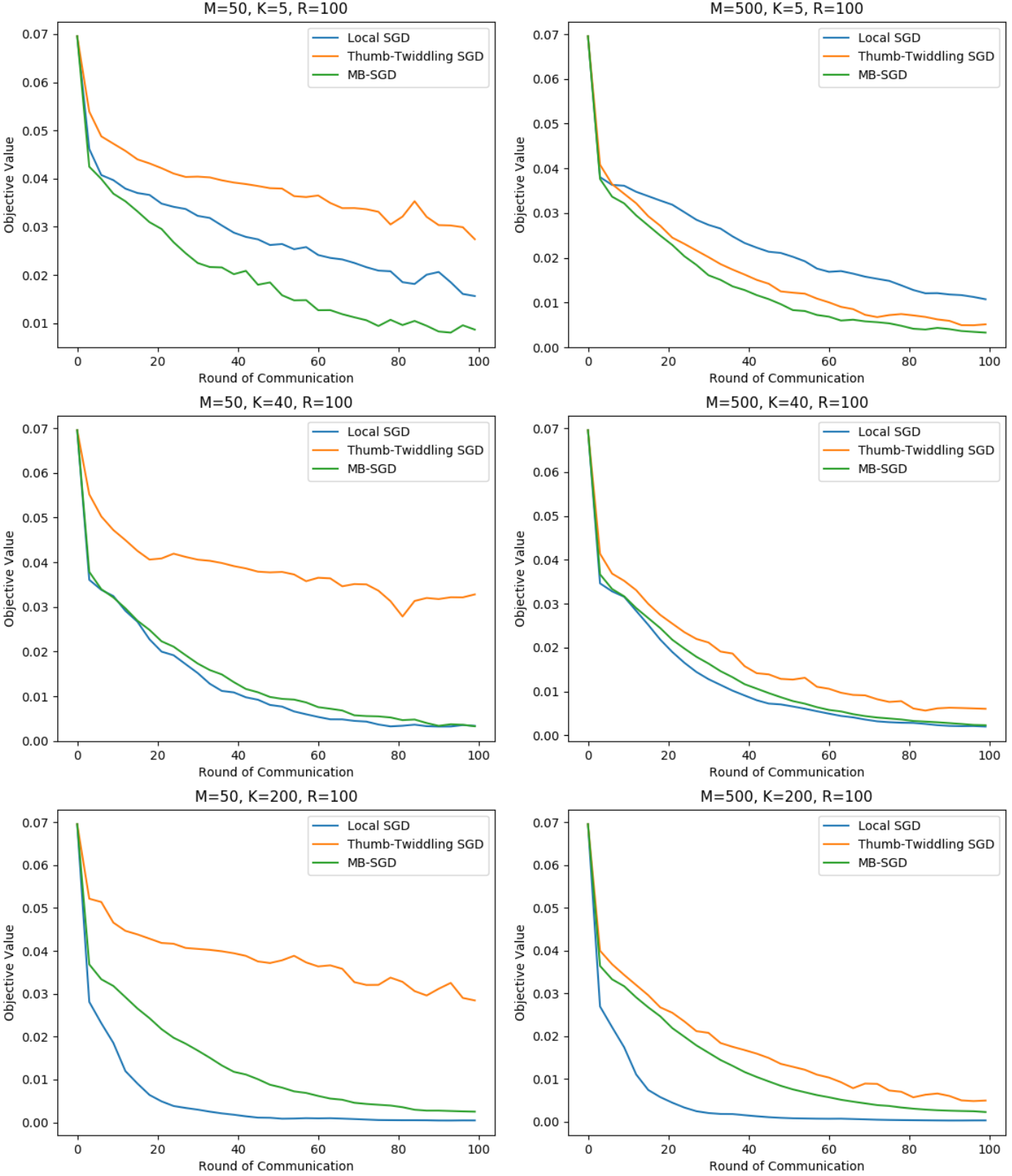
Refer to caption
Figure 1: We constructed a dataset of 50000 points in ℝ25\mathbb{R}^{25} with the iith coordinate of each point distributed independently according to a Gaussian distribution 𝒩⁡(0,10i2)\mathcal{N}(0,\frac{10}{i^{2}}). The labels are generated via ℙ⁡[y=1|x]=σ⁡(min⁡{⟨w1∗,x⟩+b1∗,⟨w2∗,x⟩+b2∗})\mathbb{P}[y=1\,|\,x]=\sigma(\min\{\left\langle w_{1}^{*},x\right\rangle+b_{1}^{*},\left\langle w_{2}^{*},x\right\rangle+b_{2}^{*}\}) for w1∗,w2∗∼𝒩⁡(0,I25×25)w_{1}^{*},w_{2}^{*}\sim\mathcal{N}(0,I_{25\times 25}) and b1∗,b2∗∼𝒩⁡(0,1)b_{1}^{*},b_{2}^{*}\sim\mathcal{N}(0,1), where σ⁡(a)=1/(1+exp⁡(−a))\sigma(a)=1/(1+\exp(-a)) is the sigmoid function, i.e. the labels correspond to an intersection of two halfspaces with label noise which increases as one approaches the decision boundary. We used each algorithm to train a linear model with a bias term to minimize the logistic loss over the 50000 points, i.e. ff is the logistic loss on one sample and 𝒟\mathcal{D} is the empirical distribution over the 50000 samples. For each MM, KK, and algorithm, we tuned the constant stepsize to minimize the loss after rr rounds of communication individually for each 1≤r≤R1\leq r\leq R. Let x𝖠,r,ηx_{\mathsf{A},r,\eta} denote algorithm 𝖠\mathsf{A}’s iterate after the rrth round of communication when using constant stepsize η\eta. The plotted lines are an approximation of g𝖠​(r)=minη⁡F⁡(x𝖠,r,η)−F⁡(x∗)g_{\mathsf{A}}(r)=\min_{\eta}F(x_{\mathsf{A},r,\eta})-F(x^{*}) for each 𝖠\mathsf{A} where the minimum is calculated using grid search on a log scale.

In order to prove Theorem 3 we constructed an artificial, but easily analyzable, situation where we could prove analytically that local SGD is worse than mini-batch. In Figure 1, we also demonstrate the behaviour empirically on a logistic regression task, by plotting the suboptimality of local SGD, minibatch SGD, and thumb-twiddling SGD iterates with optimally tuned stepsizes. As is predicted by Theorem 3, we see local SGD goes from performing worse than minibatch in the small K=5K=5 regime, but improving relative to the other algorithms as KK increases to 4040 and then 200200, when local SGD is far superior to minibatch. For each fixed KK, increasing MM causes thumb-twiddling SGD to improve relative to minibatch SGD, but does not have a significant effect on local SGD, which is consistent with introducing a bias which depends on KK but not on MM. This highlights that the “problematic regime” for local SGD is where there are few iterations per round.

6 Future work

In this paper, we provided the first analysis of local SGD showing improvement over minibatch SGD in a natural setting, but also demonstrated that local SGD can sometimes be worse than minibatch SGD, and is certainly not optimal.

As can be seen from Table 1, our upper and lower bounds for local SGD are still not tight. The first term depends on K1/3K^{1/3} versus K2/3K^{2/3}—we believe the correct behaviour might be in between, namely K\sqrt{K}, matching the bias of KK-step SGD. The exact worst case behaviour of local SGD is therefore not yet resolved.

But beyond obtaining a precise analysis of local SGD, our paper highlights a more important challenge: we see that local SGD is definitely not optimal, and does not even always improve over minibatch SGD. Can we suggest an optimal algorithm in this setting? Or at least a method that combines the advantages of both local SGD and minibatch SGD and enjoys guarantees that dominate both? Our work motivates developing such an algorithm, which might also have benefits in regimes where local SGD is already better than minibatch SGD.

To answer this question will require new upper bounds and perhaps also new lower bounds. Looking to the analysis of local AC-SA for quadratic objectives in Corollary 1, we might hope to design an algorithm which achieves error

𝔼​F​(x^)−F⁡(x∗)≤O⁡(H​B2(K​R)2+σ​BM​K​R)\mathbb{E}F(\hat{x})-F(x^{*})\leq O\left(\frac{HB^{2}}{(KR)^{2}}+\frac{\sigma B}{\sqrt{MKR}}\right) (13)

for general convex objectives. That is, an algorithm which combines the optimization term for K​RKR steps of accelerated gradient descent with the optimal statistical term. If this were possible, it would match the lower bound of Woodworth et al. 2018 and therefore be optimal with respect to this communication structure.

Acknowledgements

This work is partially supported by NSF-CCF/BSF award 1718970/2016741, NSF-DMS 1547396, and a Google Faculty Research Award. BW is supported by a Google PhD Fellowship. Part of this work was done while NS was visiting Google. Work by SS was done while visiting TTIC.

References

  • Coppola [2015] Greg Coppola. Iterative parameter mixing for distributed large-margin training of structured predictors for natural language processing. PhD thesis, The University of Edinburgh, 2015.
  • Cotter et al. [2011] Andrew Cotter, Ohad Shamir, Nati Srebro, and Karthik Sridharan. Better mini-batch algorithms via accelerated gradient methods. In J. Shawe-Taylor, R. S. Zemel, P. L. Bartlett, F. Pereira, and K. Q. Weinberger, editors, Advances in Neural Information Processing Systems 24, pages 1647–1655. Curran Associates, Inc., 2011.
  • Dekel et al. [2012] Ofer Dekel, Ran Gilad-Bachrach, Ohad Shamir, and Lin Xiao. Optimal distributed online prediction using mini-batches. Journal of Machine Learning Research, 13(Jan):165–202, 2012.
  • Dieuleveut and Patel [2019] Aymeric Dieuleveut and Kumar Kshitij Patel. Communication trade-offs for local-sgd with large step size. In Advances in Neural Information Processing Systems, pages 13579–13590, 2019.
  • Duchi et al. [2011] John Duchi, Elad Hazan, and Yoram Singer. Adaptive subgradient methods for online learning and stochastic optimization. Journal of Machine Learning Research, 12(Jul):2121–2159, 2011.
  • Ghadimi and Lan [2013] Saeed Ghadimi and Guanghui Lan. Optimal stochastic approximation algorithms for strongly convex stochastic composite optimization, ii: shrinking procedures and optimal algorithms. SIAM Journal on Optimization, 23(4):2061–2089, 2013.
  • Godichon-Baggioni and Saadane [2017] Antoine Godichon-Baggioni and Sofiane Saadane. On the rates of convergence of parallelized averaged stochastic gradient algorithms. arXiv preprint arXiv:1710.07926, 2017.
  • Haddadpour et al. [2019a] Farzin Haddadpour, Mohammad Mahdi Kamani, Mehrdad Mahdavi, and Viveck Cadambe. Local sgd with periodic averaging: Tighter analysis and adaptive synchronization. In Advances in Neural Information Processing Systems, pages 11080–11092, 2019a.
  • Haddadpour et al. [2019b] Farzin Haddadpour, Mohammad Mahdi Kamani, Mehrdad Mahdavi, and Viveck Cadambe. Trading redundancy for communication: Speeding up distributed sgd for non-convex optimization. In International Conference on Machine Learning, pages 2545–2554, 2019b.
  • Jain et al. [2017] Prateek Jain, Praneeth Netrapalli, Sham M Kakade, Rahul Kidambi, and Aaron Sidford. Parallelizing stochastic gradient descent for least squares regression: mini-batching, averaging, and model misspecification. The Journal of Machine Learning Research, 18(1):8258–8299, 2017.
  • Kairouz et al. [2019] Peter Kairouz, H. Brendan McMahan, Brendan Avent, Aurélien Bellet, Mehdi Bennis, Arjun Nitin Bhagoji, Keith Bonawitz, Zachary Charles, Graham Cormode, Rachel Cummings, Rafael G. L. D’Oliveira, Salim El Rouayheb, David Evans, Josh Gardner, Zachary Garrett, Adrià Gascón, Badih Ghazi, Phillip B. Gibbons, Marco Gruteser, Zaid Harchaoui, Chaoyang He, Lie He, Zhouyuan Huo, Ben Hutchinson, Justin Hsu, Martin Jaggi, Tara Javidi, Gauri Joshi, Mikhail Khodak, Jakub Konečný, Aleksandra Korolova, Farinaz Koushanfar, Sanmi Koyejo, Tancrède Lepoint, Yang Liu, Prateek Mittal, Mehryar Mohri, Richard Nock, Ayfer Özgür, Rasmus Pagh, Mariana Raykova, Hang Qi, Daniel Ramage, Ramesh Raskar, Dawn Song, Weikang Song, Sebastian U. Stich, Ziteng Sun, Ananda Theertha Suresh, Florian Tramèr, Praneeth Vepakomma, Jianyu Wang, Li Xiong, Zheng Xu, Qiang Yang, Felix X. Yu, Han Yu, and Sen Zhao. Advances and open problems in federated learning, 2019.
  • Karimireddy et al. [2019] Sai Praneeth Karimireddy, Satyen Kale, Mehryar Mohri, Sashank J Reddi, Sebastian U Stich, and Ananda Theertha Suresh. SCAFFOLD: Stochastic controlled averaging for on-device federated learning. arXiv preprint arXiv:1910.06378, 2019.
  • Khaled et al. [2019] Ahmed Khaled, Konstantin Mishchenko, and Peter Richtárik. Better communication complexity for local sgd. arXiv preprint arXiv:1909.04746, 2019.
  • Li et al. [2014] Mu Li, Tong Zhang, Yuqiang Chen, and Alexander J Smola. Efficient mini-batch training for stochastic optimization. In Proceedings of the 20th ACM SIGKDD international conference on Knowledge discovery and data mining, pages 661–670. ACM, 2014.
  • Lin et al. [2018] Tao Lin, Sebastian U Stich, Kumar Kshitij Patel, and Martin Jaggi. Don’t use large mini-batches, use local sgd. arXiv preprint arXiv:1808.07217, 2018.
  • McMahan and Streeter [2010] H. Brendan McMahan and Matthew J. Streeter. Adaptive bound optimization for online convex optimization. In COLT 2010 - The 23rd Conference on Learning Theory, Haifa, Israel, June 27-29, 2010, pages 244–256, 2010. URL http://colt2010.haifa.il.ibm.com/papers/COLT2010proceedings.pdf#page=252.
  • McMahan et al. [2016] H Brendan McMahan, Eider Moore, Daniel Ramage, Seth Hampson, et al. Communication-efficient learning of deep networks from decentralized data. arXiv preprint arXiv:1602.05629, 2016.
  • Nemirovsky and Yudin [1983] Arkadii Semenovich Nemirovsky and David Borisovich Yudin. Problem complexity and method efficiency in optimization. 1983.
  • Rosenblatt and Nadler [2016] Jonathan D Rosenblatt and Boaz Nadler. On the optimality of averaging in distributed statistical learning. Information and Inference: A Journal of the IMA, 5(4):379–404, 2016.
  • [20] Ohad Shamir and Nathan Srebro. Distributed stochastic optimization and learning. In 2014 52nd Annual Allerton Conference on Communication, Control, and Computing (Allerton), pages 850–857. IEEE.
  • Shamir et al. [2014] Ohad Shamir, Nati Srebro, and Tong Zhang. Communication-efficient distributed optimization using an approximate newton-type method. In International conference on machine learning, pages 1000–1008, 2014.
  • Simchowitz [2018] Max Simchowitz. On the randomized complexity of minimizing a convex quadratic function. arXiv preprint arXiv:1807.09386, 2018.
  • Stich [2018] Sebastian U Stich. Local sgd converges fast and communicates little. arXiv preprint arXiv:1805.09767, 2018. URL https://arxiv.org/abs/1805.09767.
  • Stich [2019] Sebastian U Stich. Unified optimal analysis of the (stochastic) gradient method. arXiv preprint arXiv:1907.04232, 2019.
  • Stich and Karimireddy [2019] Sebastian U Stich and Sai Praneeth Karimireddy. The error-feedback framework: Better rates for sgd with delayed gradients and compressed communication. arXiv preprint arXiv:1909.05350, 2019.
  • Vandenberghe [2019] Lieven Vandenberghe. Lecture notes 1 for optimization methods for large-scale systems, 2019.
  • Wang et al. [2017] Jialei Wang, Weiran Wang, and Nathan Srebro. Memory and communication efficient distributed stochastic optimization with minibatch-prox. arXiv preprint arXiv:1702.06269, 2017. URL https://arxiv.org/abs/1702.06269.
  • Wang and Joshi [2018] Jianyu Wang and Gauri Joshi. Cooperative sgd: A unified framework for the design and analysis of communication-efficient sgd algorithms. arXiv preprint arXiv:1808.07576, 2018.
  • Woodworth et al. [2018] Blake Woodworth, Jialei Wang, Brendan McMahan, and Nathan Srebro. Graph oracle models, lower bounds, and gaps for parallel stochastic optimization. arXiv preprint arXiv:1805.10222, 2018. URL https://arxiv.org/abs/1805.10222.
  • Yu et al. [2019] Hao Yu, Sen Yang, and Shenghuo Zhu. Parallel restarted sgd with faster convergence and less communication: Demystifying why model averaging works for deep learning. In Proceedings of the AAAI Conference on Artificial Intelligence, volume 33, pages 5693–5700, 2019.
  • Zhang et al. [2016] Jian Zhang, Christopher De Sa, Ioannis Mitliagkas, and Christopher Ré. Parallel sgd: When does averaging help? arXiv preprint arXiv:1606.07365, 2016.
  • Zhang et al. [2012] Yuchen Zhang, Martin J Wainwright, and John C Duchi. Communication-efficient algorithms for statistical optimization. In Advances in Neural Information Processing Systems, pages 1502–1510, 2012.
  • Zhang et al. [2013a] Yuchen Zhang, John Duchi, and Martin Wainwright. Divide and conquer kernel ridge regression. In Conference on learning theory, pages 592–617, 2013a.
  • Zhang et al. [2013b] Yuchen Zhang, John C Duchi, and Martin J Wainwright. Communication-efficient algorithms for statistical optimization. The Journal of Machine Learning Research, 14(1):3321–3363, 2013b.
  • Zhou and Cong [2018] Fan Zhou and Guojing Cong. On the convergence properties of a k-step averaging stochastic gradient descent algorithm for nonconvex optimization. In Proceedings of the Twenty-Seventh International Joint Conference on Artificial Intelligence, IJCAI-18, pages 3219–3227. International Joint Conferences on Artificial Intelligence Organization, 7 2018. doi: 10.24963/ijcai.2018/447. URL https://doi.org/10.24963/ijcai.2018/447.
  • Zinkevich et al. [2010] Martin Zinkevich, Markus Weimer, Lihong Li, and Alex J Smola. Parallelized stochastic gradient descent. In Advances in neural information processing systems, pages 2595–2603, 2010.

Appendix A Comparisons Between Existing Local SGD Analyses and Minibatch SGD

In this section, we describe the derivation of the entries in Table 1 for the cases in which it is not obvious. In particular, these previous analyses were stated based on different assumptions (stronger as well as weaker) which need to be reconciled with ours. Since local SGD is often analyzed in the strongly convex setting (or with weaker assumptions that are implied by strong convexity), we will make use of the following fact: If an algorithm guarantees error at most ϵ⁡(λ)\epsilon(\lambda) when applied to a λ\lambda-strongly convex function, then we can apply the algorithm to F⁡(x)+λ2​‖x‖2F(x)+\frac{\lambda}{2}\|x\|^{2} in order to ensure error ϵ⁡(λ)+λ2​‖x∗‖2\epsilon(\lambda)+\frac{\lambda}{2}\|x^{*}\|^{2}. This applies for any λ>0\lambda>0, so we can actually infer that the algorithm, in fact, guarantees error at most minλ>0⁡ϵ⁡(λ)+λ2​‖x∗‖2\min_{\lambda>0}\epsilon(\lambda)+\frac{\lambda}{2}\|x^{*}\|^{2}.

Since our purpose is to show that these analyses are dominated by minibatch SGD, the entries in the table are, in some sense, the most optimistic interpretation of the bounds stated in the paper. For example, if error ϵ1​(λ)+ϵ2​(λ)\epsilon_{1}(\lambda)+\epsilon_{2}(\lambda) is guaranteed for strongly convex functions, we actually enter 12​minλ>0​ϵ1​(λ)+λ2​‖x∗‖2+12​minλ>0​ϵ2​(λ)+λ2​‖x∗‖2\frac{1}{2}\min_{\lambda>0}\epsilon_{1}(\lambda)+\frac{\lambda}{2}\|x^{*}\|^{2}+\frac{1}{2}\min_{\lambda>0}\epsilon_{2}(\lambda)+\frac{\lambda}{2}\|x^{*}\|^{2} into the table, which is a lower bound on the actual guarantee.

Reference Setting Best Convergence rate (i.e., 𝔼⁡[F⁡(xo​u​t​p​u​t)−F⁡(x⋆)]≲\mathbb{E}\left[{F(x^{output})-F(x^{\star})}\right]\lesssim)
Stich 2018 SC σ2λ​M​K​R+H​σ2λ2​M​K2​R2+H⁡(H2​B2+σ2)λ2​R2+H3​(H2​B2+σ2)λ4​K3​R3+H2​B2+σ2λ​R3\frac{\sigma^{2}}{\lambda MKR}+\frac{H\sigma^{2}}{\lambda^{2}MK^{2}R^{2}}+\frac{H(H^{2}B^{2}+\sigma^{2})}{\lambda^{2}R^{2}}+\frac{H^{3}(H^{2}B^{2}+\sigma^{2})}{\lambda^{4}K^{3}R^{3}}+\frac{H^{2}B^{2}+\sigma^{2}}{\lambda R^{3}}
Non-SC σ​B(M​K​R)1/2+H​B2​(1+(H−1​B−1​σ)2/3)R2/3+H​B2​(1+(H−1​B−1​σ)2/5)(K​R)3/5+H​B2+B​σR3/2\frac{\sigma B}{(MKR)^{1/2}}+\frac{HB^{2}\left(1+(H^{-1}B^{-1}\sigma)^{2/3}\right)}{R^{2/3}}+\frac{HB^{2}\left(1+(H^{-1}B^{-1}\sigma)^{2/5}\right)}{(KR)^{3/5}}+\frac{HB^{2}+B\sigma}{R^{3/2}}
Stich and Karimireddy 2019 SC H​K​M​B2​exp⁡(−λ​R10​H​M)+σ2λ​M​K​RHKMB^{2}\exp\left(-\frac{\lambda R}{10HM}\right)+\frac{\sigma^{2}}{\lambda MKR}
Non-SC H​M​B2R+σ​BM​K​R\frac{HMB^{2}}{R}+\frac{\sigma B}{\sqrt{MKR}}
Khaled et al. 2019 SC H​B2K2​R2+H​σ2λ2​M​K​R+H2​σ2λ3​K​R2\frac{HB^{2}}{K^{2}R^{2}}+\frac{H\sigma^{2}}{\lambda^{2}MKR}+\frac{H^{2}\sigma^{2}}{\lambda^{3}KR^{2}}
Non-SC H​B2K​R​M+σ2H​K​R​M+σ2​MH​R\frac{HB^{2}}{\sqrt{KRM}}+\frac{\sigma^{2}}{H\sqrt{KRM}}+\frac{\sigma^{2}M}{HR}
Table 2: Best convergence rates up to constants in previous analyses under our assumptions.

For reference, we restate the worst-case guarantee of minibatch SGD:

ϵMB-SGD≍H​B2R+σ​BM​K​R\epsilon_{\textrm{MB-SGD}}\asymp\frac{HB^{2}}{R}+\frac{\sigma B}{\sqrt{MKR}} (14)

A.1 Stich 2018

The paper makes the same assumptions as us but, in addition, assumes that the stochastic gradients are uniformly bounded, i.e. 𝔼z∼𝒟​[‖∇f​(x,z)‖2]≤G2,∀x\underset{z\sim\mathcal{D}}{\mathbb{E}}\left[\|\nabla f(x;z)\|^{2}\right]\leq G^{2},\ \forall x. We relax this assumption by noting the following,

𝔼z∼𝒟​[‖∇f​(x,z)‖2]\displaystyle\underset{z\sim\mathcal{D}}{\mathbb{E}}\left[\|\nabla f(x;z)\|^{2}\right] =𝔼z∼𝒟​[‖∇f​(x,z)−∇f​(x⋆,z)+∇f​(x⋆,z)−∇F​(x⋆)‖2]\displaystyle=\underset{z\sim\mathcal{D}}{\mathbb{E}}\left[\|\nabla f(x;z)-\nabla f(x^{\star};z)+\nabla f(x^{\star};z)-\nabla F(x^{\star})\|^{2}\right] (15)
≲𝔼z∼𝒟​[‖∇f​(x,z)−∇f​(x⋆,z)‖2]+𝔼z∼𝒟​[‖∇f​(x⋆,z)−∇F​(x⋆)‖2]\displaystyle\lesssim\underset{z\sim\mathcal{D}}{\mathbb{E}}\left[\|\nabla f(x;z)-\nabla f(x^{\star};z)\|^{2}\right]+\underset{z\sim\mathcal{D}}{\mathbb{E}}\left[\|\nabla f(x^{\star};z)-\nabla F(x^{\star})\|^{2}\right] (16)
≲H2​‖x−x⋆‖2+σ2\displaystyle\lesssim H^{2}\|x-x^{\star}\|^{2}+\sigma^{2} (17)
≲H2​‖x⋆‖2+σ2\displaystyle\lesssim H^{2}\|x^{\star}\|^{2}+\sigma^{2} (18)
≤H2​B2+σ2\displaystyle\leq H^{2}B^{2}+\sigma^{2} (19)

In the last step we make the optimistic assumption that the iterates stray no farther from x∗x^{*} than they were at initialization, i.e. ‖x0−x∗‖≤B\|x_{0}-x^{*}\|\leq B. This may not be true, so this bound is optimistic. On the other hand, it is clear that one cannot generally upper bound 𝔼z∼𝒟​[‖∇f​(x,z)‖2]\underset{z\sim\mathcal{D}}{\mathbb{E}}\left[\|\nabla f(x;z)\|^{2}\right] any tighter than this in our setting. Since our goal is anyways to show that the analysis of Stich 2018 is deficient, we continue using the bound (19). This immediately gives the result for the strongly-convex setting in table 2. For the non-strongly setting we extend their result by optimizing each term separately as ϵ⁡(λ)+λ2​B2\epsilon(\lambda)+\frac{\lambda}{2}B^{2} and ignore the constants.

A.2 Stich and Karimireddy 2019

The paper relaxes the convexity assumption, by assuming F is λ⋆\lambda^{\star}-quasi convex, i.e., ∀x​F​(x⋆)≤F⁡(x)+⟨∇F,x⋆−x⟩+λ⋆2​‖x−x⋆‖2\forall x\ F(x^{\star})\leq F(x)+\left\langle\nabla F,\,x^{\star}-x\right\rangle+\frac{\lambda^{\star}}{2}\|x-x^{\star}\|^{2}. This condition can also hold for certain non-convex functions and is implied by λ⋆\lambda^{\star}-strong convexity. Besides they assume HH-smoothness of FF and multiplicative noise for the stochastic gradients, i.e., 𝔼z∼𝒟​[‖∇f​(x,z)−∇F​(x)‖2]≤N​‖x−x⋆‖2+σ⋆2\underset{z\sim\mathcal{D}}{\mathbb{E}}\left[\|\nabla f(x;z)-\nabla F(x)\|^{2}\right]\leq N\|x-x^{\star}\|^{2}+\sigma_{\star}^{2}. The latter assumption is a relaxation of the uniform upper bound on the variance of the stochastic gradients, which we have assumed. Thus to compare to their result we set N=0N=0 upper bounding the stochastic variance by σ2\sigma^{2} and use the strong convexity constant λ\lambda instead of λ⋆\lambda^{\star}. For the non-strongly convex setting we use their rate, along with our uniform variance bound. Besides they use specific learning rate and averaging schedules to optimize their rates. Both these rates are given in Table 2. For the general convex setting, we believe their dependence in MM is poor and is improved upon by our upper bound in Section 4.

A.3 Khaled et al. 2019

The relevant analysis from Khaled et al. 2019 is given in their Corollary 2, which is their only analysis that upper bounds the error in terms of the objective function suboptimality and in the setting where each machine receives i.i.d. stochastic gradients. Their Corollary 2 states that when M≤K​RM\leq KR, the error is bounded by66 6 There is a typo in their statement which omits the factor of HH (LL in their notation) from the numerator of the first term.

ϵL-SGD≤H​B2M​K​R+σ2H​M​K​R+σ2​MH​R\epsilon_{\textrm{L-SGD}}\leq\frac{HB^{2}}{\sqrt{MKR}}+\frac{\sigma^{2}}{H\sqrt{MKR}}+\frac{\sigma^{2}M}{HR} (20)

In the case where H=B=σ2=1H=B=\sigma^{2}=1, it is clear that this is strictly worse than minibatch SGD since MR>1R\frac{M}{R}>\frac{1}{R}. However, consider the case of arbitrary HH, BB and σ2\sigma^{2} and suppose Khaled et al. 2019’s guarantee is less than σ​BK​R\frac{\sigma B}{\sqrt{KR}}, in which case

H​B2M​K​R≤σ​BK​R⟹M≥H2​B2σ2⟹σ2​MH​R≥H​B2R\frac{HB^{2}}{\sqrt{MKR}}\leq\frac{\sigma B}{\sqrt{KR}}\implies M\geq\frac{H^{2}B^{2}}{\sigma^{2}}\implies\frac{\sigma^{2}M}{HR}\geq\frac{HB^{2}}{R} (21)

Consequently, (20) is either greater than σ​BK​R\frac{\sigma B}{\sqrt{KR}} or greater than H​B2R\frac{HB^{2}}{R}. This does not mean that their upper bound is worse than minibatch SGD. However, it is worse than minibatch SGD unless σ​BK​R≤H​B2R\frac{\sigma B}{\sqrt{KR}}\leq\frac{HB^{2}}{R}.

If we interrogate what this regime corresponds to, we see that it is actually a trivial regime where K​RKR steps of serial SGD, which achieves error H​B2K​R+σ​BK​R≤H​B2R\frac{HB^{2}}{KR}+\frac{\sigma B}{\sqrt{KR}}\leq\frac{HB^{2}}{R}, is actually better than minibatch SGD. That is, rather than implementing minibatch SGD distributed across the MM machines, we are actually better off just ignoring M−1M-1 of the available machines and doing serial SGD. If this is really the right thing to do, then there was never any need for parallelism in the first place, and thus there is no reason to use local SGD, which performs no better than serial SGD in this case anyways.

Appendix B Proofs from Section 3

See 1

Proof.

We will show that the average of the iterates at any particular time x¯t=1M​∑m=1Mxtm\bar{x}_{t}=\frac{1}{M}\sum_{m=1}^{M}x_{t}^{m} evolves according to 𝒜\mathcal{A} with a lower variance stochastic gradient, even though this average iterate is not explicitly computed by the algorithm at every step. It is easily confirmed from (6) that

x¯t+1\displaystyle\bar{x}_{t+1} =1M​∑m′=1Mℒ2(t)​(x1m′,…,xtm′,∇f​(ℒ1(t)​(x1m′,…,xtm′),ztm′))\displaystyle=\frac{1}{M}\sum_{m^{\prime}=1}^{M}\mathcal{L}^{(t)}_{2}\left(x_{1}^{m^{\prime}},\dots,x_{t}^{m^{\prime}},\nabla f\left(\mathcal{L}^{(t)}_{1}\left(x_{1}^{m^{\prime}},\dots,x_{t}^{m^{\prime}}\right);z_{t}^{m^{\prime}}\right)\right) (22)
=ℒ2(t)​(x¯1,…,x¯t,1M​∑m′=1M∇f​(ℒ1(t)​(x1m′,…,xtm′),ztm′))\displaystyle=\mathcal{L}^{(t)}_{2}\left(\bar{x}_{1},\dots,\bar{x}_{t},\frac{1}{M}\sum_{m^{\prime}=1}^{M}\nabla f\left(\mathcal{L}^{(t)}_{1}\left(x_{1}^{m^{\prime}},\dots,x_{t}^{m^{\prime}}\right);z_{t}^{m^{\prime}}\right)\right) (23)

where we used that ℒ2(t)\mathcal{L}^{(t)}_{2} is linear. We will now show that 1M​∑m′=1M∇f​(ℒ1(t)​(x1m′,…,xtm′),ztm′)\frac{1}{M}\sum_{m^{\prime}=1}^{M}\nabla f\left(\mathcal{L}^{(t)}_{1}\left(x_{1}^{m^{\prime}},\dots,x_{t}^{m^{\prime}}\right);z_{t}^{m^{\prime}}\right) is an unbiased estimate of ∇F​(ℒ1(t)​(x¯1,…,x¯t))\nabla F\left(\mathcal{L}^{(t)}_{1}\left(\bar{x}_{1},\dots,\bar{x}_{t}\right)\right) with variance bounded by σ2M\frac{\sigma^{2}}{M}. Therefore, x¯t+1\bar{x}_{t+1} is updated exactly according to 𝒜\mathcal{A} with a lower variance stochastic gradient.

By the linearity of ℒ1(t)\mathcal{L}^{(t)}_{1} and ∇F\nabla F

𝔼⁡[1M​∑m′=1M∇f​(ℒ1(t)​(x1m′,…,xtm′),ztm′)]=1M​∑m′=1M∇F​(ℒ1(t)​(x1m′,…,xtm′))=∇F​(ℒ1(t)​(x¯1,…,x¯t))\mathbb{E}\left[\frac{1}{M}\sum_{m^{\prime}=1}^{M}\nabla f\left(\mathcal{L}^{(t)}_{1}\left(x_{1}^{m^{\prime}},\dots,x_{t}^{m^{\prime}}\right);z_{t}^{m^{\prime}}\right)\right]=\frac{1}{M}\sum_{m^{\prime}=1}^{M}\nabla F\left(\mathcal{L}^{(t)}_{1}\left(x_{1}^{m^{\prime}},\dots,x_{t}^{m^{\prime}}\right)\right)=\nabla F\left(\mathcal{L}^{(t)}_{1}\left(\bar{x}_{1},\dots,\bar{x}_{t}\right)\right) (24)

Furthermore, since the ztmz_{t}^{m} on each machine are independent, and supx𝔼​‖∇f​(x,z)−∇F​(x)‖2≤σ2\sup_{x}\mathbb{E}\left\|\nabla f(x;z)-\nabla F(x)\right\|^{2}\leq\sigma^{2},

𝔼​‖1M​∑m′=1M∇f​(ℒ1(t)​(x1m′,…,xtm′),ztm′)−𝔼⁡[1M​∑m′=1M∇f​(ℒ1(t)​(x1m′,…,xtm′),ztm′)]‖2=1M2​∑m=1M𝔼​‖∇f​(ℒ1(t)​(x1m,…,xtm),ztm)−∇F​(ℒ1(t)​(x1m,…,xtm))‖2≤σ2M\mathbb{E}\left\|\frac{1}{M}\sum_{m^{\prime}=1}^{M}\nabla f\left(\mathcal{L}^{(t)}_{1}\left(x_{1}^{m^{\prime}},\dots,x_{t}^{m^{\prime}}\right);z_{t}^{m^{\prime}}\right)-\mathbb{E}\left[\frac{1}{M}\sum_{m^{\prime}=1}^{M}\nabla f\left(\mathcal{L}^{(t)}_{1}\left(x_{1}^{m^{\prime}},\dots,x_{t}^{m^{\prime}}\right);z_{t}^{m^{\prime}}\right)\right]\right\|^{2}\\ =\frac{1}{M^{2}}\sum_{m=1}^{M}\mathbb{E}\left\|\nabla f\left(\mathcal{L}^{(t)}_{1}\left(x_{1}^{m},\dots,x_{t}^{m}\right);z_{t}^{m}\right)-\nabla F\left(\mathcal{L}^{(t)}_{1}\left(x_{1}^{m},\dots,x_{t}^{m}\right)\right)\right\|^{2}\leq\frac{\sigma^{2}}{M} (25)

∎

See 1

Proof.

It is easily confirmed that SGD and AC-SA [6] are linear update algorithms, which allows us to apply Theorem 1. In addition, Simchowitz 2018 shows that any randomized algorithm that accesses an deterministic first order oracle at most TT times will have error at least c​H​B2T2\frac{cHB^{2}}{T^{2}} in the worst case for an HH-smooth, convex quadratic objective, for some universal constant cc. Therefore, the first term of local-AC-SA’s guarantee cannot be improved. The second term of the guarantee also cannot be improved [18]—in fact, this term cannot be improved even by an algorithm which is allowed to make M​K​RMKR sequential calls to a stochastic gradient oracle. ∎

Appendix C Proof of Theorem 2

Before we prove Theorem 2, we will introduce some notation. Recall that the objective is of the form F⁡(x):=𝔼z∼𝒟​[f⁡(x,z)]F(x):=\mathbb{E}_{z\sim\mathcal{D}}\left[f(x;z)\right]. Let ηt\eta_{t} denote the stepsize used for the ttth overall iteration. Let xtmx_{t}^{m} denote the ttth iterate on the mmth machine, and let x¯t=1M​∑m=1Mxtm\bar{x}_{t}=\frac{1}{M}\sum_{m=1}^{M}x_{t}^{m} denote the averaged ttth iterate. The vector x¯t\bar{x}_{t} may not actually be computed by the algorithm, but it will be central to our analysis. We will use ∇f​(xtm,ztm)\nabla f(x_{t}^{m};z_{t}^{m}) to denote the stochastic gradient computed at xtmx_{t}^{m} by the mmth machine at iteration tt, and gt=1M​∑m=1M∇f​(xtm,ztm)g_{t}=\frac{1}{M}\sum_{m=1}^{M}\nabla f(x_{t}^{m};z_{t}^{m}) will denote the average of the stochastic gradients computed at time tt. Finally, let g¯t=1M​∑m=1M∇F​(xtm)\bar{g}_{t}=\frac{1}{M}\sum_{m=1}^{M}\nabla F(x_{t}^{m}) denote the average of the full gradients computed at the individual iterates.

Lemma 1 (See Lemma 3.1 [23]).

Let FF be HH-smooth and λ\lambda-strongly convex, let
supx𝔼​‖∇f​(x,z)−∇F​(x)‖2≤σ2\sup_{x}\mathbb{E}\left\|\nabla f(x;z)-\nabla F(x)\right\|^{2}\leq\sigma^{2}, and let ηt≤14​H\eta_{t}\leq\frac{1}{4H}, then the iterates of local SGD satisfy

𝔼⁡[F⁡(x¯t)−F∗]≤(2ηt−2​λ)​𝔼​‖x¯t−x∗‖2−2ηt​𝔼​‖x¯t+1−x∗‖2+2​ηt​σ2M+4​HM​∑m=1M𝔼​‖x¯t−xtm‖2\mathbb{E}\left[F(\bar{x}_{t})-F^{*}\right]\leq\left(\frac{2}{\eta_{t}}-2\lambda\right)\mathbb{E}\left\|\bar{x}_{t}-x^{*}\right\|^{2}-\frac{2}{\eta_{t}}\mathbb{E}\left\|\bar{x}_{t+1}-x^{*}\right\|^{2}+\frac{2\eta_{t}\sigma^{2}}{M}+\frac{4H}{M}\sum_{m=1}^{M}\mathbb{E}\left\|\bar{x}_{t}-x_{t}^{m}\right\|^{2}
Proof.

This proof is nearly identical to the proof of Lemma 3.1 due to Stich 2018, and we claim no technical innovation here. We include it in order to be self-contained.

We begin by analyzing the distance of x¯t+1\bar{x}_{t+1} from the optimum. Below, expectations are taken over the all of the random variables {ztm}\left\{z_{t}^{m}\right\} which determine the iterates {xtm}\left\{x_{t}^{m}\right\}.

𝔼​‖x¯t+1−x∗‖2\displaystyle\mathbb{E}\left\|\bar{x}_{t+1}-x^{*}\right\|^{2}
=𝔼​‖x¯t−ηt​gt−x∗‖2\displaystyle=\mathbb{E}\left\|\bar{x}_{t}-\eta_{t}g_{t}-x^{*}\right\|^{2} (26)
=𝔼⁡‖x¯t−x∗‖+ηt2​𝔼​‖g¯t‖2+ηt2​𝔼​‖gt−g¯t‖2−2​ηt​𝔼​⟨x¯t−x∗,g¯t⟩\displaystyle=\mathbb{E}\left\|\bar{x}_{t}-x^{*}\right\|+\eta_{t}^{2}\mathbb{E}\left\|\bar{g}_{t}\right\|^{2}+\eta_{t}^{2}\mathbb{E}\left\|g_{t}-\bar{g}_{t}\right\|^{2}-2\eta_{t}\mathbb{E}\left\langle\bar{x}_{t}-x^{*},\bar{g}_{t}\right\rangle (27)
≤𝔼⁡‖x¯t−x∗‖+ηt2​𝔼​‖g¯t‖2+ηt2​σ2M−2​ηtM​∑m=1M𝔼⁡⟨x¯t−x∗,∇f​(xtm,ztm)⟩\displaystyle\leq\mathbb{E}\left\|\bar{x}_{t}-x^{*}\right\|+\eta_{t}^{2}\mathbb{E}\left\|\bar{g}_{t}\right\|^{2}+\frac{\eta_{t}^{2}\sigma^{2}}{M}-\frac{2\eta_{t}}{M}\sum_{m=1}^{M}\mathbb{E}\left\langle\bar{x}_{t}-x^{*},\nabla f(x_{t}^{m};z_{t}^{m})\right\rangle (28)
=𝔼⁡‖x¯t−x∗‖+ηt2​𝔼​‖g¯t‖2+ηt2​σ2M−2​ηtM​∑m=1M[𝔼⁡⟨xtm−x∗,∇F​(xtm)⟩+𝔼⁡⟨x¯t−xtm,∇F​(xtm)⟩]\displaystyle=\mathbb{E}\left\|\bar{x}_{t}-x^{*}\right\|+\eta_{t}^{2}\mathbb{E}\left\|\bar{g}_{t}\right\|^{2}+\frac{\eta_{t}^{2}\sigma^{2}}{M}-\frac{2\eta_{t}}{M}\sum_{m=1}^{M}\left[\mathbb{E}\left\langle x_{t}^{m}-x^{*},\nabla F(x_{t}^{m})\right\rangle+\mathbb{E}\left\langle\bar{x}_{t}-x_{t}^{m},\nabla F(x_{t}^{m})\right\rangle\right] (29)

For the second equality, we used that 𝔼⁡[gt−g¯t]=0\mathbb{E}\left[g_{t}-\bar{g}_{t}\right]=0; for the first inequality, we used that 𝔼​‖gt−g¯t‖2=𝔼​‖1M​∑m=1M∇f​(xtm,ztm)−∇F​(xtm)‖2≤σ2M\mathbb{E}\left\|g_{t}-\bar{g}_{t}\right\|^{2}=\mathbb{E}\left\|\frac{1}{M}\sum_{m=1}^{M}\nabla f(x_{t}^{m};z_{t}^{m})-\nabla F(x_{t}^{m})\right\|^{2}\leq\frac{\sigma^{2}}{M} since the individual stochastic gradient estimates are independent; and for the final equality, we used that ztmz_{t}^{m} is independent of x¯t\bar{x}_{t}.

For any vectors vmv_{m}, ‖∑m=1Mvm‖2≤M​∑m=1M‖vm‖2\left\|\sum_{m=1}^{M}v_{m}\right\|^{2}\leq M\sum_{m=1}^{M}\left\|v_{m}\right\|^{2}. In addition, for any point xx and HH-smooth FF, ‖∇F​(x)‖2≤2​H​(F⁡(x)−F⁡(x∗))\left\|\nabla F(x)\right\|^{2}\leq 2H(F(x)-F(x^{*})), thus

ηt2𝔼‖g¯t‖2≤ηt2M∑m=1M‖1M∇F(xtm)‖2≤2​H​ηt2M∑m=1MF(xtm)−F(x∗)\eta_{t}^{2}\mathbb{E}\left\|\bar{g}_{t}\right\|^{2}\leq\eta_{t}^{2}M\sum_{m=1}^{M}\left\|\frac{1}{M}\nabla F(x_{t}^{m})\right\|^{2}\leq\frac{2H\eta_{t}^{2}}{M}\sum_{m=1}^{M}F(x_{t}^{m})-F(x^{*}) (30)

By the λ\lambda-strong convexity of FF, we have that

−2​ηtM∑m=1M⟨xtm−x∗,∇F(xtm)⟩≤−2​ηtM∑m=1M[F(xtm)−F(x∗)+λ2‖xtm−x∗‖2]≤−2​ηtM∑m=1M[F(xtm)−F(x∗)]−ληt‖x¯t−x∗‖2-\frac{2\eta_{t}}{M}\sum_{m=1}^{M}\left\langle x_{t}^{m}-x^{*},\nabla F(x_{t}^{m})\right\rangle\leq-\frac{2\eta_{t}}{M}\sum_{m=1}^{M}\left[F(x_{t}^{m})-F(x^{*})+\frac{\lambda}{2}\left\|x_{t}^{m}-x^{*}\right\|^{2}\right]\\ \leq-\frac{2\eta_{t}}{M}\sum_{m=1}^{M}\left[F(x_{t}^{m})-F(x^{*})\right]-\lambda\eta_{t}\left\|\bar{x}_{t}-x^{*}\right\|^{2} (31)

Finally, using the fact that for any vectors a,ba,b and any γ>0\gamma>0, 2​⟨a,b⟩≤γ​‖a‖2+γ−1​‖b‖22\left\langle a,b\right\rangle\leq\gamma\|a\|^{2}+\gamma^{-1}\|b\|^{2} we have

−2​ηt​⟨x¯t−xtm,∇F​(xtm)⟩≤ηt​γ​‖x¯t−xtm‖2+ηtγ​‖∇F​(xtm)‖2≤ηt​γ​‖x¯t−xtm‖2+2​H​ηtγ​[F⁡(xtm)−F⁡(x∗)]-2\eta_{t}\left\langle\bar{x}_{t}-x_{t}^{m},\nabla F(x_{t}^{m})\right\rangle\leq\eta_{t}\gamma\left\|\bar{x}_{t}-x_{t}^{m}\right\|^{2}+\frac{\eta_{t}}{\gamma}\left\|\nabla F(x_{t}^{m})\right\|^{2}\leq\eta_{t}\gamma\left\|\bar{x}_{t}-x_{t}^{m}\right\|^{2}+\frac{2H\eta_{t}}{\gamma}[F(x_{t}^{m})-F(x^{*})] (32)

Combining these with (29), we conclude that for γ=2​H\gamma=2H

𝔼​‖x¯t+1−x∗‖2\displaystyle\mathbb{E}\left\|\bar{x}_{t+1}-x^{*}\right\|^{2} ≤(1−λ​ηt)​𝔼​‖x¯t−x∗‖−2​ηt​(1−H​ηt)M​∑m=1M𝔼⁡[F⁡(xtm)−F⁡(x∗)]+ηt2​σ2M\displaystyle\leq\left(1-\lambda\eta_{t}\right)\mathbb{E}\left\|\bar{x}_{t}-x^{*}\right\|-\frac{2\eta_{t}\left(1-H\eta_{t}\right)}{M}\sum_{m=1}^{M}\mathbb{E}\left[F(x_{t}^{m})-F(x^{*})\right]+\frac{\eta_{t}^{2}\sigma^{2}}{M}
+ηtM∑m=1M[2H𝔼‖x¯t−xtm‖2+𝔼[F(xtm)−F(x∗)]]\displaystyle\qquad\qquad+\frac{\eta_{t}}{M}\sum_{m=1}^{M}\left[2H\mathbb{E}\left\|\bar{x}_{t}-x_{t}^{m}\right\|^{2}+\mathbb{E}\left[F(x_{t}^{m})-F(x^{*})\right]\right] (33)
=(1−λ​ηt)​𝔼​‖x¯t−x∗‖−ηt​(1−2​H​ηt)M​∑m=1M𝔼⁡[F⁡(xtm)−F⁡(x∗)]\displaystyle=\left(1-\lambda\eta_{t}\right)\mathbb{E}\left\|\bar{x}_{t}-x^{*}\right\|-\frac{\eta_{t}\left(1-2H\eta_{t}\right)}{M}\sum_{m=1}^{M}\mathbb{E}\left[F(x_{t}^{m})-F(x^{*})\right]
+ηt2​σ2M+2​H​ηtM​∑m=1M𝔼​‖x¯t−xtm‖2\displaystyle\qquad\qquad+\frac{\eta_{t}^{2}\sigma^{2}}{M}+\frac{2H\eta_{t}}{M}\sum_{m=1}^{M}\mathbb{E}\left\|\bar{x}_{t}-x_{t}^{m}\right\|^{2} (34)

By the convexity of FF and the fact that ηt≤14​H\eta_{t}\leq\frac{1}{4H}, this implies

𝔼​‖x¯t+1−x∗‖2\displaystyle\mathbb{E}\left\|\bar{x}_{t+1}-x^{*}\right\|^{2} ≤(1−λ​ηt)​𝔼​‖x¯t−x∗‖−ηt2​𝔼​[F⁡(x¯t)−F⁡(x∗)]+ηt2​σ2M+2​H​ηtM​∑m=1M𝔼​‖x¯t−xtm‖2\displaystyle\leq\left(1-\lambda\eta_{t}\right)\mathbb{E}\left\|\bar{x}_{t}-x^{*}\right\|-\frac{\eta_{t}}{2}\mathbb{E}\left[F(\bar{x}_{t})-F(x^{*})\right]+\frac{\eta_{t}^{2}\sigma^{2}}{M}+\frac{2H\eta_{t}}{M}\sum_{m=1}^{M}\mathbb{E}\left\|\bar{x}_{t}-x_{t}^{m}\right\|^{2} (35)

Rearranging completes the proof. ∎

We will proceed to bound the final term in Lemma 1 more tightly than was done by Stich 2018, which allows us to improve on their upper bound. To do so, we will use the following technical lemmas:

Lemma 2 (Co-Coercivity of the Gradient).

For any HH-smooth and convex FF, and any xx, and yy

‖∇F​(x)−∇F​(y)‖2≤H⁡⟨∇F​(x)−∇F​(y),x−y⟩\left\|\nabla F(x)-\nabla F(y)\right\|^{2}\leq H\left\langle\nabla F(x)-\nabla F(y),\,x-y\right\rangle

and

‖∇F​(x)−∇F​(y)‖2≤2​H​(F⁡(x)−F⁡(y)−⟨∇F​(y),x−y⟩)\left\|\nabla F(x)-\nabla F(y)\right\|^{2}\leq 2H\left(F(x)-F(y)-\left\langle\nabla F(y),\,x-y\right\rangle\right)
Proof.

This proof follows closely from [26]. Define the HH-smooth, convex functions

Fx​(z)=F⁡(z)−⟨∇F​(x),z⟩andFy​(z)=F⁡(z)−⟨∇F​(y),z⟩F_{x}(z)=F(z)-\left\langle\nabla F(x),\,z\right\rangle\qquad\textrm{and}\qquad F_{y}(z)=F(z)-\left\langle\nabla F(y),\,z\right\rangle (36)

By setting the gradients of these convex functions equal to zero, it is clear that xx minimizes FxF_{x} and yy minimizes FyF_{y}. For any HH-smooth and convex FF, for any zz, ‖∇F​(z)‖2≤2​H​(F⁡(z)−minx⁡F⁡(x))\left\|\nabla F(z)\right\|^{2}\leq 2H(F(z)-\min_{x}F(x)), therefore,

F⁡(y)−F⁡(x)−⟨∇F​(x),y−x⟩\displaystyle F(y)-F(x)-\left\langle\nabla F(x),\,y-x\right\rangle =Fx​(y)−Fx​(x)\displaystyle=F_{x}(y)-F_{x}(x) (37)
≥12​H​‖∇Fx​(y)‖2\displaystyle\geq\frac{1}{2H}\left\|\nabla F_{x}(y)\right\|^{2} (38)
=12​H​‖∇F​(y)−∇F​(x)‖2\displaystyle=\frac{1}{2H}\left\|\nabla F(y)-\nabla F(x)\right\|^{2} (39)

Similarly,

F⁡(x)−F⁡(y)−⟨∇F​(y),x−y⟩≥12​H​‖∇F​(y)−∇F​(x)‖2F(x)-F(y)-\left\langle\nabla F(y),\,x-y\right\rangle\geq\frac{1}{2H}\left\|\nabla F(y)-\nabla F(x)\right\|^{2} (40)

This is the second claim of the Lemma, and combining these last two inequalities proves the first claim. ∎

Lemma 3 (See Lemma 6 [12]).

Let FF be any HH-smooth and λ\lambda-strongly convex function, and let η≤1H\eta\leq\frac{1}{H}. Then for any x,yx,y

‖x−η∇F(x)−y+η∇F(y)‖2≤(1−λη)‖x−y‖2\left\|x-\eta\nabla F(x)-y+\eta\nabla F(y)\right\|^{2}\leq\left(1-\lambda\eta\right)\left\|x-y\right\|^{2}
Proof.

This Lemma and its proof are essentially identical to [12, Lemma 6], we include it here in order to keep our results self-contained, and we are more explicit about the steps used.

‖x−η∇F(x)−y+η∇F(y)‖2\displaystyle\left\|x-\eta\nabla F(x)-y+\eta\nabla F(y)\right\|^{2} =‖x−y‖2+η2​‖∇F​(x)−∇F​(y)‖2−2​η​⟨∇F​(x)−∇F​(y),x−y⟩\displaystyle=\left\|x-y\right\|^{2}+\eta^{2}\left\|\nabla F(x)-\nabla F(y)\right\|^{2}-2\eta\left\langle\nabla F(x)-\nabla F(y),\,x-y\right\rangle (41)
≤‖x−y‖2+η2​H​⟨∇F​(x)−∇F​(y),x−y⟩−2​η​⟨∇F​(x)−∇F​(y),x−y⟩\displaystyle\leq\left\|x-y\right\|^{2}+\eta^{2}H\left\langle\nabla F(x)-\nabla F(y),\,x-y\right\rangle-2\eta\left\langle\nabla F(x)-\nabla F(y),\,x-y\right\rangle (42)

where the inequality follows from Lemma 2. Since η​H≤1\eta H\leq 1, we further conclude that

‖x−η∇F(x)−y+η∇F(y)‖2≤‖x−y‖2−η⟨∇F(x)−∇F(y),x−y⟩\left\|x-\eta\nabla F(x)-y+\eta\nabla F(y)\right\|^{2}\leq\left\|x-y\right\|^{2}-\eta\left\langle\nabla F(x)-\nabla F(y),\,x-y\right\rangle (43)

Finally, by the λ\lambda-strong convexity of FF

⟨∇F​(x),x−y⟩≥F⁡(x)−F⁡(y)+λ2​‖x−y‖2\displaystyle\left\langle\nabla F(x),\,x-y\right\rangle\geq F(x)-F(y)+\frac{\lambda}{2}\left\|x-y\right\|^{2} (44)
−⟨∇F​(y),x−y⟩≥F⁡(y)−F⁡(x)+λ2​‖x−y‖2\displaystyle-\left\langle\nabla F(y),\,x-y\right\rangle\geq F(y)-F(x)+\frac{\lambda}{2}\left\|x-y\right\|^{2} (45)

Combining these, we conclude

‖x−η∇F(x)−y+η∇F(y)‖2\displaystyle\left\|x-\eta\nabla F(x)-y+\eta\nabla F(y)\right\|^{2} ≤‖x−y‖2−η⁡⟨∇F​(x)−∇F​(y),x−y⟩\displaystyle\leq\left\|x-y\right\|^{2}-\eta\left\langle\nabla F(x)-\nabla F(y),\,x-y\right\rangle (46)
≤‖x−y‖2−η​λ​‖x−y‖2\displaystyle\leq\left\|x-y\right\|^{2}-\eta\lambda\left\|x-y\right\|^{2} (47)

which completes the proof. ∎

Lemma 4.

For any tt and m≠m′m\neq m^{\prime}

𝔼​‖xtm−x¯t‖2≤M−1M​𝔼​‖xtm−xtm′‖2\mathbb{E}\left\|x_{t}^{m}-\bar{x}_{t}\right\|^{2}\leq\frac{M-1}{M}\mathbb{E}\left\|x_{t}^{m}-x_{t}^{m^{\prime}}\right\|^{2}
Proof.

First, we note that xt1,…,xtMx_{t}^{1},\dots,x_{t}^{M} are identically distributed. Therefore,

𝔼​‖xtm−x¯t‖2\displaystyle\mathbb{E}\left\|x_{t}^{m}-\bar{x}_{t}\right\|^{2} =𝔼​‖xtm−1M​∑m′=1Mxtm′‖2\displaystyle=\mathbb{E}\left\|x_{t}^{m}-\frac{1}{M}\sum_{m^{\prime}=1}^{M}x_{t}^{m^{\prime}}\right\|^{2} (48)
=1M2​𝔼​‖1M​∑m′≠mxtm−xtm′‖2\displaystyle=\frac{1}{M^{2}}\mathbb{E}\left\|\frac{1}{M}\sum_{m^{\prime}\neq m}x_{t}^{m}-x_{t}^{m^{\prime}}\right\|^{2} (49)
=1M2​[∑m′≠m𝔼​‖xtm−xtm′‖2+∑m′≠m,m′′≠m,m′≠m′′𝔼⁡⟨xtm−xtm′,xtm−xtm′′⟩]\displaystyle=\frac{1}{M^{2}}\left[\sum_{m^{\prime}\neq m}\mathbb{E}\left\|x_{t}^{m}-x_{t}^{m^{\prime}}\right\|^{2}+\sum_{m^{\prime}\neq m,m^{\prime\prime}\neq m,m^{\prime}\neq m^{\prime\prime}}\mathbb{E}\left\langle x_{t}^{m}-x_{t}^{m^{\prime}},\,x_{t}^{m}-x_{t}^{m^{\prime\prime}}\right\rangle\right] (50)
≤1M2​[(M−1)​𝔼​‖xtm−xtm′‖2+∑m′≠m,m′′≠m,m′≠m′′𝔼​‖xtm−xtm′‖2​𝔼​‖xtm−xtm′′‖2]\displaystyle\leq\frac{1}{M^{2}}\left[(M-1)\mathbb{E}\left\|x_{t}^{m}-x_{t}^{m^{\prime}}\right\|^{2}+\sum_{m^{\prime}\neq m,m^{\prime\prime}\neq m,m^{\prime}\neq m^{\prime\prime}}\sqrt{\mathbb{E}\left\|x_{t}^{m}-x_{t}^{m^{\prime}}\right\|^{2}\mathbb{E}\left\|x_{t}^{m}-x_{t}^{m^{\prime\prime}}\right\|^{2}}\right] (51)
=1M2​[(M−1)​𝔼​‖xtm−xtm′‖2+2​(M−12)​𝔼​‖xtm−xtm′‖2]\displaystyle=\frac{1}{M^{2}}\left[(M-1)\mathbb{E}\left\|x_{t}^{m}-x_{t}^{m^{\prime}}\right\|^{2}+2\binom{M-1}{2}\mathbb{E}\left\|x_{t}^{m}-x_{t}^{m^{\prime}}\right\|^{2}\right] (52)
=(M−1)2M2​𝔼​‖xtm−xtm′‖2\displaystyle=\frac{(M-1)^{2}}{M^{2}}\mathbb{E}\left\|x_{t}^{m}-x_{t}^{m^{\prime}}\right\|^{2} (53)
≤M−1M​𝔼​‖xtm−xtm′‖2\displaystyle\leq\frac{M-1}{M}\mathbb{E}\left\|x_{t}^{m}-x_{t}^{m^{\prime}}\right\|^{2} (54)

∎

Lemma 5.

Under the conditions of Lemma 1, with the additional condition that the sequence of stepsizes η1,η2,…\eta_{1},\eta_{2},\dots is non-increasing and ηt≤1H\eta_{t}\leq\frac{1}{H} for all tt, for any tt and any mm

𝔼​‖xtm−x¯t‖2≤2​(M−1)​(K−1)​ηt−K+1∧02​σ2M\mathbb{E}\left\|x_{t}^{m}-\bar{x}_{t}\right\|^{2}\leq\frac{2(M-1)(K-1)\eta_{t-K+1\land 0}^{2}\sigma^{2}}{M}

If ηt=2λ⁡(a+t+1)\eta_{t}=\frac{2}{\lambda(a+t+1)}, then it further satisfies

𝔼​‖xtm−x¯t‖2≤2​(M−1)​(K−1)​ηt−12​σ2M\mathbb{E}\left\|x_{t}^{m}-\bar{x}_{t}\right\|^{2}\leq\frac{2(M-1)(K-1)\eta_{t-1}^{2}\sigma^{2}}{M}
Proof.

By Lemma 4, we can upper bound

𝔼​‖xtm−x¯t‖2≤M−1M​𝔼​‖xtm−xtm′‖2\mathbb{E}\left\|x_{t}^{m}-\bar{x}_{t}\right\|^{2}\leq\frac{M-1}{M}\mathbb{E}\left\|x_{t}^{m}-x_{t}^{m^{\prime}}\right\|^{2} (55)

for all tt and m≠m′m\neq m^{\prime}. In addition,

𝔼​‖xtm−xtm′‖2\displaystyle\mathbb{E}\left\|x_{t}^{m}-x_{t}^{m^{\prime}}\right\|^{2} =𝔼‖xt−1m−ηt−1∇f(xt−1m;zt−1m)−xt−1m′+ηt−1∇f(xt−1m′;zt−1m′)‖2\displaystyle=\mathbb{E}\left\|x_{t-1}^{m}-\eta_{t-1}\nabla f(x_{t-1}^{m};z_{t-1}^{m})-x_{t-1}^{m^{\prime}}+\eta_{t-1}\nabla f(x_{t-1}^{m^{\prime}};z_{t-1}^{m^{\prime}})\right\|^{2} (56)
≤𝔼‖xt−1m−ηt−1∇F(xt−1m)−xt−1m′+ηt−1∇F(xt−1m′)‖2+2ηt−12σ2\displaystyle\leq\mathbb{E}\left\|x_{t-1}^{m}-\eta_{t-1}\nabla F(x_{t-1}^{m})-x_{t-1}^{m^{\prime}}+\eta_{t-1}\nabla F(x_{t-1}^{m^{\prime}})\right\|^{2}+2\eta_{t-1}^{2}\sigma^{2} (57)
≤(1−λ​ηt−1)​𝔼​‖xt−1m−xt−1m′‖2+2​ηt−12​σ2\displaystyle\leq\left(1-\lambda\eta_{t-1}\right)\mathbb{E}\left\|x_{t-1}^{m}-x_{t-1}^{m^{\prime}}\right\|^{2}+2\eta_{t-1}^{2}\sigma^{2} (58)

where for the final inequality we used Lemma 3 and the fact that the stepsizes are less than 1H\frac{1}{H},. Since the iterates are averaged every KK iterations, for each tt, there must be a t0t_{0} with 0≤t−t0≤K−10\leq t-t_{0}\leq K-1 such that xt0m=xt0m′x_{t_{0}}^{m}=x_{t_{0}}^{m^{\prime}}. Therefore, we can unroll the recurrence above to conclude that

𝔼​‖xtm−xtm′‖2≤∑i=t0t−12​ηi2​σ2​∏j=i+1t−1(1−λ​ηj)≤2​σ2​∑i=t0t−1ηi2\mathbb{E}\left\|x_{t}^{m}-x_{t}^{m^{\prime}}\right\|^{2}\leq\sum_{i=t_{0}}^{t-1}2\eta_{i}^{2}\sigma^{2}\prod_{j=i+1}^{t-1}\left(1-\lambda\eta_{j}\right)\leq 2\sigma^{2}\sum_{i=t_{0}}^{t-1}\eta_{i}^{2} (59)

where we define ∑i=abci=0\sum_{i=a}^{b}c_{i}=0 and ∏i=abci=1\prod_{i=a}^{b}c_{i}=1 for all a>ba>b and all {ci}i∈ℕ\{c_{i}\}_{i\in\mathbb{N}}. Therefore, for any non-increasing stepsizes, we conclude

𝔼​‖xtm−x¯t‖2≤2​ηt−K+1∧02​σ2​(M−1)​(K−1)M\mathbb{E}\left\|x_{t}^{m}-\bar{x}_{t}\right\|^{2}\leq\frac{2\eta_{t-K+1\land 0}^{2}\sigma^{2}(M-1)(K-1)}{M} (60)

This implies the first claim.

In the special case ηt=2λ⁡(a+t+1)\eta_{t}=\frac{2}{\lambda\left(a+t+1\right)}, we have

𝔼​‖xtm−xm′‖2\displaystyle\mathbb{E}\left\|x_{t}^{m}-x^{m^{\prime}}\right\|^{2} ≤2​σ2​∑i=t0t−1ηi2​∏j=i+1t−1(1−λ​ηj)\displaystyle\leq 2\sigma^{2}\sum_{i=t_{0}}^{t-1}\eta_{i}^{2}\prod_{j=i+1}^{t-1}\left(1-\lambda\eta_{j}\right) (61)
=2​σ2​∑i=t0t−1ηi2​∏j=i+1t−1(a+j−1a+j+1)\displaystyle=2\sigma^{2}\sum_{i=t_{0}}^{t-1}\eta_{i}^{2}\prod_{j=i+1}^{t-1}\left(\frac{a+j-1}{a+j+1}\right) (62)
=2​σ2​ηt−12+2​σ2​ηt−22​(a+t−2)a+t+2​σ2​∑i=t0t−3ηi2​(a+i)​(a+i+1)(a+t−1)​(a+t)\displaystyle=2\sigma^{2}\eta_{t-1}^{2}+\frac{2\sigma^{2}\eta_{t-2}^{2}(a+t-2)}{a+t}+2\sigma^{2}\sum_{i=t_{0}}^{t-3}\eta_{i}^{2}\frac{(a+i)(a+i+1)}{(a+t-1)(a+t)} (63)
=2​σ2​ηt−12​(1+(a+t)​(a+t−2)(a+t−1)2+∑i=t0t−3(a+i)​(a+t)(a+t−1)​(a+i+1))\displaystyle=2\sigma^{2}\eta_{t-1}^{2}\left(1+\frac{(a+t)(a+t-2)}{(a+t-1)^{2}}+\sum_{i=t_{0}}^{t-3}\frac{(a+i)(a+t)}{(a+t-1)(a+i+1)}\right) (64)
≤2​σ2​ηt−12​(t−t0)\displaystyle\leq 2\sigma^{2}\eta_{t-1}^{2}\left(t-t_{0}\right) (65)
≤2​(K−1)​σ2​ηt−12\displaystyle\leq 2(K-1)\sigma^{2}\eta_{t-1}^{2} (66)

This implies the second claim. ∎

Next, we show that Local SGD is always at least as good as K​RKR steps of sequential SGD. To do so, we use the following result from Stich 2019:

Lemma 6 (Lemma 3 [24]).

For any recurrence of the form

rt+1≤(1−a​γt)​rt−b​γt​st+c​γt2r_{t+1}\leq(1-a\gamma_{t})r_{t}-b\gamma_{t}s_{t}+c\gamma_{t}^{2}

with a,b>0a,b>0, there exists a sequence 0<γt≤1d0<\gamma_{t}\leq\frac{1}{d} and weights wt>0w_{t}>0 such that

bWT​∑t=0T[st​wt+a​rt+1]≤32​d​r0​exp⁡(−a​T2​d)+36​ca​T\frac{b}{W_{T}}\sum_{t=0}^{T}\left[s_{t}w_{t}+ar_{t+1}\right]\leq 32dr_{0}\exp\left(-\frac{aT}{2d}\right)+\frac{36c}{aT}

where WT:=∑t=0TwtW_{T}:=\sum_{t=0}^{T}w_{t}.

We now argue that Local SGD is never worse than K​RKR steps of sequential SGD:

Lemma 7.

Let (f,𝒟)∈ℱ⁡(H,λ,B,σ2)(f,\mathcal{D})\in\mathcal{F}(H,\lambda,B,\sigma^{2}). When λ=0\lambda=0, an appropriate average of the iterates of Local SGD with an optimally tuned constant stepsize satisfies for a universal constant cc

F⁡(x^)−F∗≤c⋅H​B2K​R+c⋅σ​BK​RF(\hat{x})-F^{*}\leq c\cdot\frac{HB^{2}}{KR}+c\cdot\frac{\sigma B}{\sqrt{KR}}

In the case λ>0\lambda>0, then an appropriate average of the iterates of Local SGD with decreasing stepsize ηt≍(λ​t)−1\eta_{t}\asymp(\lambda t)^{-1} satisfies for a universal constant cc

F⁡(x^)−F∗≤c⋅H​B2​exp⁡(−λ​K​R4​H)+c⋅σ2λ​K​RF(\hat{x})-F^{*}\leq c\cdot HB^{2}\exp\left(-\frac{\lambda KR}{4H}\right)+c\cdot\frac{\sigma^{2}}{\lambda KR}
Proof.

Define T:=K​RT:=KR and consider the (t+1)(t+1)st iterate on some machine mm, xt+1mx_{t+1}^{m}. If t+1modK≠0t+1\mod K\neq 0, then xt+1m=xtm−ηt∇f(xtm;ztm)x_{t+1}^{m}=x_{t}^{m}-\eta_{t}\nabla f(x_{t}^{m};z_{t}^{m}). In this case, for ηt≤12​H\eta_{t}\leq\frac{1}{2H}

𝔼​‖xt+1m−x∗‖2\displaystyle\mathbb{E}\left\|x_{t+1}^{m}-x^{*}\right\|^{2} =𝔼‖xtm−ηt∇f(xtm;ztm)−x∗‖2\displaystyle=\mathbb{E}\left\|x_{t}^{m}-\eta_{t}\nabla f(x_{t}^{m};z_{t}^{m})-x^{*}\right\|^{2} (67)
=𝔼​‖xtm−x∗‖2+ηt2​𝔼​‖∇f​(xtm,ztm)‖2−2​ηt​𝔼​⟨∇f​(xtm,ztm),xtm−x∗⟩\displaystyle=\mathbb{E}\left\|x_{t}^{m}-x^{*}\right\|^{2}+\eta_{t}^{2}\mathbb{E}\left\|\nabla f(x_{t}^{m};z_{t}^{m})\right\|^{2}-2\eta_{t}\mathbb{E}\left\langle\nabla f(x_{t}^{m};z_{t}^{m}),\,x_{t}^{m}-x^{*}\right\rangle (68)
≤𝔼​‖xtm−x∗‖2+ηt2​σ2+ηt2​𝔼​‖∇F​(xtm)‖2−2​ηt​𝔼​⟨∇F​(xtm),xtm−x∗⟩\displaystyle\leq\mathbb{E}\left\|x_{t}^{m}-x^{*}\right\|^{2}+\eta_{t}^{2}\sigma^{2}+\eta_{t}^{2}\mathbb{E}\left\|\nabla F(x_{t}^{m})\right\|^{2}-2\eta_{t}\mathbb{E}\left\langle\nabla F(x_{t}^{m}),\,x_{t}^{m}-x^{*}\right\rangle (69)
≤𝔼​‖xtm−x∗‖2+ηt2​σ2+2​H​ηt2​𝔼​[F⁡(xtm)−F∗]−2​ηt​𝔼​[F⁡(xtm)−F∗+λ2​‖xtm−x∗‖2]\displaystyle\leq\mathbb{E}\left\|x_{t}^{m}-x^{*}\right\|^{2}+\eta_{t}^{2}\sigma^{2}+2H\eta_{t}^{2}\mathbb{E}\left[F(x_{t}^{m})-F^{*}\right]-2\eta_{t}\mathbb{E}\left[F(x_{t}^{m})-F^{*}+\frac{\lambda}{2}\left\|x_{t}^{m}-x^{*}\right\|^{2}\right] (70)
=(1−λ​ηt)​𝔼​‖xtm−x∗‖2+ηt2​σ2−2​ηt​(1−H​ηt)​𝔼​[F⁡(xtm)−F∗]\displaystyle=(1-\lambda\eta_{t})\mathbb{E}\left\|x_{t}^{m}-x^{*}\right\|^{2}+\eta_{t}^{2}\sigma^{2}-2\eta_{t}(1-H\eta_{t})\mathbb{E}\left[F(x_{t}^{m})-F^{*}\right] (71)
⟹𝔼⁡[F⁡(xtm)−F∗]\displaystyle\implies\mathbb{E}\left[F(x_{t}^{m})-F^{*}\right] ≤(1ηt−λ)​𝔼​‖xtm−x∗‖2−1ηt​𝔼​‖xt+1m−x∗‖2+ηt​σ2\displaystyle\leq\left(\frac{1}{\eta_{t}}-\lambda\right)\mathbb{E}\left\|x_{t}^{m}-x^{*}\right\|^{2}-\frac{1}{\eta_{t}}\mathbb{E}\left\|x_{t+1}^{m}-x^{*}\right\|^{2}+\eta_{t}\sigma^{2} (72)

Here, for the first inequality we used the variance bound on the stochastic gradients; for the second inequality we used the HH-smoothness and λ\lambda-strong convexity of FF; and for the final inequality we used that H​ηt≤12H\eta_{t}\leq\frac{1}{2} and rearranged.

If, on the other hand, t+1modK=0t+1\mod K=0, then xt+1m=1M∑m′=1Mxtm′−ηt∇f(xtm′;ztm′)x_{t+1}^{m}=\frac{1}{M}\sum_{m^{\prime}=1}^{M}x_{t}^{m^{\prime}}-\eta_{t}\nabla f(x_{t}^{m^{\prime}};z_{t}^{m^{\prime}}). Since the local iterates on the different machines are identically distributed,

𝔼​‖xt+1m−x∗‖2\displaystyle\mathbb{E}\left\|x_{t+1}^{m}-x^{*}\right\|^{2} =𝔼‖1M∑m′=1Mxtm′−ηt∇f(xtm′;ztm′)−x∗‖2\displaystyle=\mathbb{E}\left\|\frac{1}{M}\sum_{m^{\prime}=1}^{M}x_{t}^{m^{\prime}}-\eta_{t}\nabla f(x_{t}^{m^{\prime}};z_{t}^{m^{\prime}})-x^{*}\right\|^{2} (73)
≤1M∑m′=1M𝔼‖xtm′−ηt∇f(xtm′;ztm′)−x∗‖2\displaystyle\leq\frac{1}{M}\sum_{m^{\prime}=1}^{M}\mathbb{E}\left\|x_{t}^{m^{\prime}}-\eta_{t}\nabla f(x_{t}^{m^{\prime}};z_{t}^{m^{\prime}})-x^{*}\right\|^{2} (74)
=𝔼‖xtm−ηt∇f(xtm;ztm)−x∗‖2\displaystyle=\mathbb{E}\left\|x_{t}^{m}-\eta_{t}\nabla f(x_{t}^{m};z_{t}^{m})-x^{*}\right\|^{2} (75)

Where for the first inequality we used Jensen’s inequality, and for the final equality we used that the local iterates are identically distributed. From here, using the same computation as above, we conclude that in either case

𝔼⁡[F⁡(xtm)−F∗]≤(1ηt−λ)​𝔼​‖xtm−x∗‖2−1ηt​𝔼​‖xt+1m−x∗‖2+ηt​σ2\mathbb{E}\left[F(x_{t}^{m})-F^{*}\right]\leq\left(\frac{1}{\eta_{t}}-\lambda\right)\mathbb{E}\left\|x_{t}^{m}-x^{*}\right\|^{2}-\frac{1}{\eta_{t}}\mathbb{E}\left\|x_{t+1}^{m}-x^{*}\right\|^{2}+\eta_{t}\sigma^{2} (76)
Weakly Convex Case λ=0\lambda=0:

Choose a constant learning rate ηt=η=min⁡{12​H,Bσ​T}\eta_{t}=\eta=\min\left\{\frac{1}{2H},\frac{B}{\sigma\sqrt{T}}\right\} and define the averaged iterate

x^=1M​T​∑m=1M∑t=1Txtm\hat{x}=\frac{1}{MT}\sum_{m=1}^{M}\sum_{t=1}^{T}x_{t}^{m} (77)

Then, by the convexity of FF:

𝔼​F​(x^)−F∗\displaystyle\mathbb{E}F(\hat{x})-F^{*} ≤1M​T​∑m=1M∑t=1T𝔼⁡[F⁡(xtm)−F∗]\displaystyle\leq\frac{1}{MT}\sum_{m=1}^{M}\sum_{t=1}^{T}\mathbb{E}\left[F(x_{t}^{m})-F^{*}\right] (78)
≤1M​T​∑m=1M∑t=1T1η​𝔼​‖xtm−x∗‖2−1η​𝔼​‖xt+1m−x∗‖2+η​σ2\displaystyle\leq\frac{1}{MT}\sum_{m=1}^{M}\sum_{t=1}^{T}\frac{1}{\eta}\mathbb{E}\left\|x_{t}^{m}-x^{*}\right\|^{2}-\frac{1}{\eta}\mathbb{E}\left\|x_{t+1}^{m}-x^{*}\right\|^{2}+\eta\sigma^{2} (79)
=‖x0−x∗‖2T​η+η​σ2\displaystyle=\frac{\left\|x_{0}-x^{*}\right\|^{2}}{T\eta}+\eta\sigma^{2} (80)
=max⁡{2​H​‖x0−x∗‖2T,σ⁡‖x0−x∗‖T}+σ⁡‖x0−x∗‖T\displaystyle=\max\left\{\frac{2H\left\|x_{0}-x^{*}\right\|^{2}}{T},\frac{\sigma\left\|x_{0}-x^{*}\right\|}{\sqrt{T}}\right\}+\frac{\sigma\left\|x_{0}-x^{*}\right\|}{\sqrt{T}} (81)
≤2​H​‖x0−x∗‖2T+2​σ​‖x0−x∗‖T\displaystyle\leq\frac{2H\left\|x_{0}-x^{*}\right\|^{2}}{T}+\frac{2\sigma\left\|x_{0}-x^{*}\right\|}{\sqrt{T}} (82)
Strongly Convex Case λ>0\lambda>0:

Rearranging (76), we see that it has the same form as the recurrence analyzed in Lemma 6 with rt=𝔼​‖xtm−x∗‖2r_{t}=\mathbb{E}\left\|x_{t}^{m}-x^{*}\right\|^{2}, st=𝔼⁡[F⁡(xtm)−F∗]s_{t}=\mathbb{E}\left[F(x_{t}^{m})-F^{*}\right], a=λa=\lambda, c=σ2c=\sigma^{2}, and γt=ηt\gamma_{t}=\eta_{t} with the requirement that ηt≤12​H\eta_{t}\leq\frac{1}{2H}, i.e. d=2​Hd=2H. Consequently, by Lemma 6, we conclude that there is a sequence of stepsizes and weights wtw_{t} such that

𝔼⁡[F⁡(1M​∑t=0K​Rwt​∑m=1M∑t=0K​Rwt​xtm)−F∗]\displaystyle\mathbb{E}\left[F\left(\frac{1}{M\sum_{t=0}^{KR}w_{t}}\sum_{m=1}^{M}\sum_{t=0}^{KR}w_{t}x_{t}^{m}\right)-F^{*}\right] ≤1M​∑t=0K​Rwt​∑m=1M∑t=0K​R𝔼⁡[F⁡(wt​xtm)−F∗]\displaystyle\leq\frac{1}{M\sum_{t=0}^{KR}w_{t}}\sum_{m=1}^{M}\sum_{t=0}^{KR}\mathbb{E}\left[F\left(w_{t}x_{t}^{m}\right)-F^{*}\right] (83)
≤64​H​𝔼​‖x0−x∗‖2​exp⁡(−λ​K​R4​H)+36​σ2λ​K​R\displaystyle\leq 64H\mathbb{E}\left\|x_{0}-x^{*}\right\|^{2}\exp\left(-\frac{\lambda KR}{4H}\right)+\frac{36\sigma^{2}}{\lambda KR} (84)

The stepsizes and weights are chosen as follows: If K​R≤2​HλKR\leq\frac{2H}{\lambda}, then ηt=12​H\eta_{t}=\frac{1}{2H} and wt=(1−λ​η)−t−1w_{t}=(1-\lambda\eta)^{-t-1}. If K​R>2​HλKR>\frac{2H}{\lambda} and t<K​R/2t<KR/2, then ηt=12​H\eta_{t}=\frac{1}{2H} and wt=0w_{t}=0. If K​R>2​HλKR>\frac{2H}{\lambda} and t≥K​R/2t\geq KR/2, then ηt=24​H+λ⁡(t−K​R/2)\eta_{t}=\frac{2}{4H+\lambda(t-KR/2)} and wt=(4​H/λ+t−K​R/2)2w_{t}=(4H/\lambda+t-KR/2)^{2}. This completes the proof. ∎

Finally, we prove our main analysis of Local SGD. Portions of the analysis of the strongly convex case follow closely the proof of [24, Lemma 3]. See 2

Proof.

We will prove the first terms in the min\min’s in Theorem in two parts, first for the convex case λ=0\lambda=0, then for the strongly convex case λ>0\lambda>0. Then, we conclude by invoking Lemma 7 showing that Local SGD is never worse than K​RKR steps of SGD on a single machine, which corresponds to the second terms in the min\min’s in the Theorem statement.

Convex Case λ=0\lambda=0:

By Lemma 1 and the first claim of Lemma 5, the mean iterate satisfies

𝔼⁡[F⁡(x¯t)−F∗]≤2ηt​𝔼​‖x¯t−x∗‖2−2ηt​𝔼​‖x¯t+1−x∗‖2+2​ηt​σ2M+8​H​(M−1)​(K−1)​ηt−K+2∧02​σ2M\mathbb{E}\left[F(\bar{x}_{t})-F^{*}\right]\leq\frac{2}{\eta_{t}}\mathbb{E}\left\|\bar{x}_{t}-x^{*}\right\|^{2}-\frac{2}{\eta_{t}}\mathbb{E}\left\|\bar{x}_{t+1}-x^{*}\right\|^{2}+\frac{2\eta_{t}\sigma^{2}}{M}+\frac{8H(M-1)(K-1)\eta_{t-K+2\land 0}^{2}\sigma^{2}}{M} (85)

Consider a fixed stepsize ηt=η\eta_{t}=\eta which will be chosen later, and consider the average of the iterates

x^=1K​R​∑t=1K​Rx¯t\hat{x}=\frac{1}{KR}\sum_{t=1}^{KR}\bar{x}_{t} (86)

By the convexity of FF,

𝔼⁡[F⁡(x^)−F∗]\displaystyle\mathbb{E}\left[F(\hat{x})-F^{*}\right] ≤1K​R​∑t=1K​R𝔼⁡[F⁡(x¯t)−F∗]\displaystyle\leq\frac{1}{KR}\sum_{t=1}^{KR}\mathbb{E}\left[F(\bar{x}_{t})-F^{*}\right] (87)
≤1K​R​∑t=1K​R[2η​𝔼​‖x¯t−x∗‖2−2η​𝔼​‖x¯t+1−x∗‖2+2​η​σ2M+8​H​(M−1)​(K−1)​η2​σ2M]\displaystyle\leq\frac{1}{KR}\sum_{t=1}^{KR}\left[\frac{2}{\eta}\mathbb{E}\left\|\bar{x}_{t}-x^{*}\right\|^{2}-\frac{2}{\eta}\mathbb{E}\left\|\bar{x}_{t+1}-x^{*}\right\|^{2}+\frac{2\eta\sigma^{2}}{M}+\frac{8H(M-1)(K-1)\eta^{2}\sigma^{2}}{M}\right] (88)
≤2​B2η​K​R+2​η​σ2M+8​H​(M−1)​(K−1)​η2​σ2M\displaystyle\leq\frac{2B^{2}}{\eta KR}+\frac{2\eta\sigma^{2}}{M}+\frac{8H(M-1)(K-1)\eta^{2}\sigma^{2}}{M} (89)

Choose as a stepsize

η={min⁡{14​H,B​Mσ​K​R}K=1​ or ​M=1min⁡{14​H,B​Mσ​K​R,(B2H​σ2​K2​R)13}Otherwise \eta=\begin{cases}\min\left\{\frac{1}{4H},\ \frac{B\sqrt{M}}{\sigma\sqrt{KR}}\right\}&K=1\textrm{ or }M=1\\ \min\left\{\frac{1}{4H},\ \frac{B\sqrt{M}}{\sigma\sqrt{KR}},\ \left(\frac{B^{2}}{H\sigma^{2}K^{2}R}\right)^{\frac{1}{3}}\right\}&\textrm{Otherwise }\end{cases} (90)

Then,

𝔼⁡[F⁡(x^)−F∗]\displaystyle\mathbb{E}\left[F(\hat{x})-F^{*}\right] ≤2​B2η​K​R+2​η​σ2M+8​H​(M−1)​(K−1)​η2​σ2M\displaystyle\leq\frac{2B^{2}}{\eta KR}+\frac{2\eta\sigma^{2}}{M}+\frac{8H(M-1)(K-1)\eta^{2}\sigma^{2}}{M} (91)
≤max⁡{8​H​B2K​R,2​σ​BM​K​R,2​(H​σ2​B4)13K1/3​R2/3}+2​σ​BM​K​R+8​(H​σ2​B4)13K1/3​R2/3\displaystyle\leq\max\left\{\frac{8HB^{2}}{KR},\ \frac{2\sigma B}{\sqrt{MKR}},\ \frac{2\left(H\sigma^{2}B^{4}\right)^{\frac{1}{3}}}{K^{1/3}R^{2/3}}\right\}+\frac{2\sigma B}{\sqrt{MKR}}+\frac{8\left(H\sigma^{2}B^{4}\right)^{\frac{1}{3}}}{K^{1/3}R^{2/3}} (92)
≤8​H​B2K​R+4​σ​BM​K​R+10​(H​σ2​B4)13K1/3​R2/3\displaystyle\leq\frac{8HB^{2}}{KR}+\frac{4\sigma B}{\sqrt{MKR}}+\frac{10\left(H\sigma^{2}B^{4}\right)^{\frac{1}{3}}}{K^{1/3}R^{2/3}} (93)
Strongly Convex Case λ>0\lambda>0:

For the strongly convex case, following Stich 2019’s proof of Lemma 6, we choose stepsizes according to the following set of cases: If K​R≤2​HλKR\leq\frac{2H}{\lambda}, then ηt=14​H\eta_{t}=\frac{1}{4H} and wt=(1−λ​η)−t−1w_{t}=(1-\lambda\eta)^{-t-1}. If K​R>2​HλKR>\frac{2H}{\lambda} and t≤K​R/2t\leq KR/2, then ηt=14​H\eta_{t}=\frac{1}{4H} and wt=0w_{t}=0. If K​R>2​HλKR>\frac{2H}{\lambda} and t>K​R/2t>KR/2, then ηt=28​H+λ⁡(t−K​R/2)\eta_{t}=\frac{2}{8H+\lambda(t-KR/2)} and wt=(8​H/λ+t−K​R/2)w_{t}=(8H/\lambda+t-KR/2). We note that in the second and third cases, the stepsize is either constant or equal to ηt=2λ⁡(a+t−K​R/2)\eta_{t}=\frac{2}{\lambda(a+t-KR/2)} (for a=8​Hλa=\frac{8H}{\lambda}) within each individual round of communication.

By Lemma 1 and the first claim of Lemma 5, during the rounds of communication for which the stepsize is constant, we have the recurrence:

𝔼​‖x¯t+1−x∗‖2≤(1−λ​ηt)​𝔼​‖x¯t−x∗‖2−ηt2​𝔼​[F⁡(x¯t)−F∗]+ηt2​σ2M+4​H​K​ηt3​σ2\mathbb{E}\left\|\bar{x}_{t+1}-x^{*}\right\|^{2}\leq\left(1-\lambda\eta_{t}\right)\mathbb{E}\left\|\bar{x}_{t}-x^{*}\right\|^{2}-\frac{\eta_{t}}{2}\mathbb{E}\left[F(\bar{x}_{t})-F^{*}\right]+\frac{\eta_{t}^{2}\sigma^{2}}{M}+4HK\eta_{t}^{3}\sigma^{2} (94)

On the other hand, during the rounds of communication in which the stepsize is decreasing, we have by Lemma 1 and the second claim of Lemma 5 that:

𝔼​‖x¯t+1−x∗‖2≤(1−λ​ηt)​𝔼​‖x¯t−x∗‖2−ηt2​𝔼​[F⁡(x¯t)−F∗]+ηt2​σ2M+4​H​K​ηt​ηt−12​σ2\mathbb{E}\left\|\bar{x}_{t+1}-x^{*}\right\|^{2}\leq\left(1-\lambda\eta_{t}\right)\mathbb{E}\left\|\bar{x}_{t}-x^{*}\right\|^{2}-\frac{\eta_{t}}{2}\mathbb{E}\left[F(\bar{x}_{t})-F^{*}\right]+\frac{\eta_{t}^{2}\sigma^{2}}{M}+4HK\eta_{t}\eta_{t-1}^{2}\sigma^{2} (95)

Furthermore, during the rounds (i.e. when t>K​Rt>KR) where the stepsize is decreasing,

ηt−12=ηt2​(a+t−K​R/2)2(a−1+t−K​R/2)2≤4​ηt2\eta_{t-1}^{2}=\eta_{t}^{2}\frac{\left(a+t-KR/2\right)^{2}}{\left(a-1+t-KR/2\right)^{2}}\leq 4\eta_{t}^{2} (96)

So, for every tt we conclude

𝔼​‖x¯t+1−x∗‖2≤(1−λ​ηt)​𝔼​‖x¯t−x∗‖2−ηt2​𝔼​[F⁡(x¯t)−F∗]+ηt2​σ2M+16​H​K​ηt3​σ2\mathbb{E}\left\|\bar{x}_{t+1}-x^{*}\right\|^{2}\leq\left(1-\lambda\eta_{t}\right)\mathbb{E}\left\|\bar{x}_{t}-x^{*}\right\|^{2}-\frac{\eta_{t}}{2}\mathbb{E}\left[F(\bar{x}_{t})-F^{*}\right]+\frac{\eta_{t}^{2}\sigma^{2}}{M}+16HK\eta_{t}^{3}\sigma^{2} (97)

First, suppose K​R>2​HλKR>\frac{2H}{\lambda}, and consider the steps during which ηt=14​H\eta_{t}=\frac{1}{4H}:

𝔼​‖x¯K​R/2−x∗‖2\displaystyle\mathbb{E}\left\|\bar{x}_{KR/2}-x^{*}\right\|^{2} ≤(1−λ4​H)​𝔼​‖x¯t−x∗‖2−18​H​𝔼​[F⁡(x¯t)−F∗]+σ216​H2​M+K​σ24​H2\displaystyle\leq\left(1-\frac{\lambda}{4H}\right)\mathbb{E}\left\|\bar{x}_{t}-x^{*}\right\|^{2}-\frac{1}{8H}\mathbb{E}\left[F(\bar{x}_{t})-F^{*}\right]+\frac{\sigma^{2}}{16H^{2}M}+\frac{K\sigma^{2}}{4H^{2}} (98)
≤(1−λ4​H)​𝔼​‖x¯t−x∗‖2+σ216​H2​M+K​σ24​H2\displaystyle\leq\left(1-\frac{\lambda}{4H}\right)\mathbb{E}\left\|\bar{x}_{t}-x^{*}\right\|^{2}+\frac{\sigma^{2}}{16H^{2}M}+\frac{K\sigma^{2}}{4H^{2}} (99)
≤(1−λ4​H)K​R/2​𝔼​‖x¯0−x∗‖2+(σ216​H2​M+K​σ24​H2)​∑t=0K​R/2−1(1−λ4​H)t\displaystyle\leq\left(1-\frac{\lambda}{4H}\right)^{KR/2}\mathbb{E}\left\|\bar{x}_{0}-x^{*}\right\|^{2}+\left(\frac{\sigma^{2}}{16H^{2}M}+\frac{K\sigma^{2}}{4H^{2}}\right)\sum_{t=0}^{KR/2-1}\left(1-\frac{\lambda}{4H}\right)^{t} (100)
≤(1−λ4​H)K​R/2​𝔼​‖x¯0−x∗‖2+4​Hλ​(σ216​H2​M+K​σ24​H2)\displaystyle\leq\left(1-\frac{\lambda}{4H}\right)^{KR/2}\mathbb{E}\left\|\bar{x}_{0}-x^{*}\right\|^{2}+\frac{4H}{\lambda}\left(\frac{\sigma^{2}}{16H^{2}M}+\frac{K\sigma^{2}}{4H^{2}}\right) (101)
≤𝔼​‖x¯0−x∗‖2​exp⁡(−λ​K​R8​H)+σ24​H​λ​M+K​σ2H​λ\displaystyle\leq\mathbb{E}\left\|\bar{x}_{0}-x^{*}\right\|^{2}\exp\left(-\frac{\lambda KR}{8H}\right)+\frac{\sigma^{2}}{4H\lambda M}+\frac{K\sigma^{2}}{H\lambda} (102)

Now, consider the remaining steps. Rearranging, we have

𝔼⁡[F⁡(x¯t)−F∗]\displaystyle\mathbb{E}\left[F(\bar{x}_{t})-F^{*}\right] ≤(2ηt−λ2)​𝔼​‖x¯t−x∗‖2−2ηt​𝔼​‖x¯t+1−x∗‖2+2​ηt​σ2M+32​H​K​ηt2​σ2\displaystyle\leq\left(\frac{2}{\eta_{t}}-\frac{\lambda}{2}\right)\mathbb{E}\left\|\bar{x}_{t}-x^{*}\right\|^{2}-\frac{2}{\eta_{t}}\mathbb{E}\left\|\bar{x}_{t+1}-x^{*}\right\|^{2}+\frac{2\eta_{t}\sigma^{2}}{M}+32HK\eta_{t}^{2}\sigma^{2} (103)

So, since ηt=2λ⁡(a+t)\eta_{t}=\frac{2}{\lambda(a+t)} where a=8​Hλ−K​R2a=\frac{8H}{\lambda}-\frac{KR}{2} and wt=(a+t)w_{t}=(a+t), we have

1WT​∑t=K​R/2K​Rwt​𝔼​[F⁡(x¯t)−F∗]\displaystyle\frac{1}{W_{T}}\sum_{t=KR/2}^{KR}w_{t}\mathbb{E}\left[F(\bar{x}_{t})-F^{*}\right]
≤1WT​∑t=K​R/2K​Rwt​[(2ηt−2​λ)​𝔼​‖x¯t−x∗‖2−2ηt​𝔼​‖x¯t+1−x∗‖2+2​ηt​σ2M+32​H​K​ηt2​σ2]\displaystyle\leq\frac{1}{W_{T}}\sum_{t=KR/2}^{KR}w_{t}\left[\left(\frac{2}{\eta_{t}}-2\lambda\right)\mathbb{E}\left\|\bar{x}_{t}-x^{*}\right\|^{2}-\frac{2}{\eta_{t}}\mathbb{E}\left\|\bar{x}_{t+1}-x^{*}\right\|^{2}+\frac{2\eta_{t}\sigma^{2}}{M}+32HK\eta_{t}^{2}\sigma^{2}\right] (104)
=1WT​∑t=K​R/2K​Rλ⁡(a+t)​(a+t−2)​𝔼​‖x¯t−x∗‖2−λ​(a+t)2​𝔼​‖x¯t+1−x∗‖2+2​σ2λ​M+32​H​K​ηt​σ2λ\displaystyle=\frac{1}{W_{T}}\sum_{t=KR/2}^{KR}\lambda(a+t)(a+t-2)\mathbb{E}\left\|\bar{x}_{t}-x^{*}\right\|^{2}-\lambda(a+t)^{2}\mathbb{E}\left\|\bar{x}_{t+1}-x^{*}\right\|^{2}+\frac{2\sigma^{2}}{\lambda M}+\frac{32HK\eta_{t}\sigma^{2}}{\lambda} (105)
≤1WT​∑t=K​R/2K​Rλ​(a+t−1)2​𝔼​‖x¯t−x∗‖2−λ​(a+t)2​𝔼​‖x¯t+1−x∗‖2+2​σ2λ​M+32​H​K​ηt​σ2λ\displaystyle\leq\frac{1}{W_{T}}\sum_{t=KR/2}^{KR}\lambda(a+t-1)^{2}\mathbb{E}\left\|\bar{x}_{t}-x^{*}\right\|^{2}-\lambda(a+t)^{2}\mathbb{E}\left\|\bar{x}_{t+1}-x^{*}\right\|^{2}+\frac{2\sigma^{2}}{\lambda M}+\frac{32HK\eta_{t}\sigma^{2}}{\lambda} (106)
≤λ​(a+K​R/2−1)2WT​𝔼​‖x¯K​R/2−x∗‖2+2​σ2​(K​R/2)WT​λ​M+64​H​K​σ2WT​λ2​∑t=K​R/2K​R1a+t\displaystyle\leq\frac{\lambda(a+KR/2-1)^{2}}{W_{T}}\mathbb{E}\left\|\bar{x}_{KR/2}-x^{*}\right\|^{2}+\frac{2\sigma^{2}(KR/2)}{W_{T}\lambda M}+\frac{64HK\sigma^{2}}{W_{T}\lambda^{2}}\sum_{t=KR/2}^{KR}\frac{1}{a+t} (107)
=λ​(8​Hλ−1)2WT​𝔼​‖x¯K​R/2−x∗‖2+2​σ2​(K​R/2)WT​λ​M+64​H​K​σ2WT​λ2​∑t′=1K​R/218​Hλ+t′\displaystyle=\frac{\lambda\left(\frac{8H}{\lambda}-1\right)^{2}}{W_{T}}\mathbb{E}\left\|\bar{x}_{KR/2}-x^{*}\right\|^{2}+\frac{2\sigma^{2}(KR/2)}{W_{T}\lambda M}+\frac{64HK\sigma^{2}}{W_{T}\lambda^{2}}\sum_{t^{\prime}=1}^{KR/2}\frac{1}{\frac{8H}{\lambda}+t^{\prime}} (108)
≤64​H2WT​λ​𝔼​‖x¯K​R/2−x∗‖2+2​σ2​(K​R/2)WT​λ​M+64​H​K​σ2WT​λ2​log⁡(e+λ​K​R4​H)\displaystyle\leq\frac{64H^{2}}{W_{T}\lambda}\mathbb{E}\left\|\bar{x}_{KR/2}-x^{*}\right\|^{2}+\frac{2\sigma^{2}(KR/2)}{W_{T}\lambda M}+\frac{64HK\sigma^{2}}{W_{T}\lambda^{2}}\log\left(e+\frac{\lambda KR}{4H}\right) (109)

Finally, we recall (102), K​R>2​HλKR>\frac{2H}{\lambda}, and note that WT=∑t=K​R/2K​Ra+t≥3​K2​R28+a​K​R2=K2​R28+4​H​K​Rλ≥8​H2λ2W_{T}=\sum_{t=KR/2}^{KR}a+t\geq\frac{3K^{2}R^{2}}{8}+\frac{aKR}{2}=\frac{K^{2}R^{2}}{8}+\frac{4HKR}{\lambda}\geq\frac{8H^{2}}{\lambda^{2}} thus

1WT​∑t=K​R/2K​Rwt​𝔼​[F⁡(x¯t)−F∗]\displaystyle\frac{1}{W_{T}}\sum_{t=KR/2}^{KR}w_{t}\mathbb{E}\left[F(\bar{x}_{t})-F^{*}\right]
≤64​H2WT​λ​(𝔼​‖x¯0−x∗‖2​exp⁡(−λ​K​R8​H)+σ24​H​λ​M+K​σ2H​λ)+2​σ2​(K​R/2)WT​λ​M+64​H​K​σ2WT​λ2​log⁡(e+λ​K​R4​H)\displaystyle\leq\frac{64H^{2}}{W_{T}\lambda}\left(\mathbb{E}\left\|\bar{x}_{0}-x^{*}\right\|^{2}\exp\left(-\frac{\lambda KR}{8H}\right)+\frac{\sigma^{2}}{4H\lambda M}+\frac{K\sigma^{2}}{H\lambda}\right)+\frac{2\sigma^{2}(KR/2)}{W_{T}\lambda M}+\frac{64HK\sigma^{2}}{W_{T}\lambda^{2}}\log\left(e+\frac{\lambda KR}{4H}\right) (110)
≤64​H2WT​λ​𝔼​‖x¯0−x∗‖2​exp⁡(−λ​K​R8​H)+16​H​σ2λ2​M​WT+64​H​K​σ2λ2​WT+8​σ2λ​M​K​R+512​H​σ2λ2​K​R2​log⁡(e+λ​K​R4​H)\displaystyle\leq\frac{64H^{2}}{W_{T}\lambda}\mathbb{E}\left\|\bar{x}_{0}-x^{*}\right\|^{2}\exp\left(-\frac{\lambda KR}{8H}\right)+\frac{16H\sigma^{2}}{\lambda^{2}MW_{T}}+\frac{64HK\sigma^{2}}{\lambda^{2}W_{T}}+\frac{8\sigma^{2}}{\lambda MKR}+\frac{512H\sigma^{2}}{\lambda^{2}KR^{2}}\log\left(e+\frac{\lambda KR}{4H}\right) (111)
≤8​λ​𝔼​‖x¯0−x∗‖2​exp⁡(−λ​K​R8​H)+4​σ2λ​M​K​R+512​H​σ2λ2​K​R2+8​σ2λ​M​K​R+512​H​σ2λ2​K​R2​log⁡(e+λ​K​R4​H)\displaystyle\leq 8\lambda\mathbb{E}\left\|\bar{x}_{0}-x^{*}\right\|^{2}\exp\left(-\frac{\lambda KR}{8H}\right)+\frac{4\sigma^{2}}{\lambda MKR}+\frac{512H\sigma^{2}}{\lambda^{2}KR^{2}}+\frac{8\sigma^{2}}{\lambda MKR}+\frac{512H\sigma^{2}}{\lambda^{2}KR^{2}}\log\left(e+\frac{\lambda KR}{4H}\right) (112)
≤8​λ​𝔼​‖x¯0−x∗‖2​exp⁡(−λ​K​R8​H)+12​σ2λ​M​K​R+512​H​σ2λ2​K​R2​log⁡(9+λ​K​RH)\displaystyle\leq 8\lambda\mathbb{E}\left\|\bar{x}_{0}-x^{*}\right\|^{2}\exp\left(-\frac{\lambda KR}{8H}\right)+\frac{12\sigma^{2}}{\lambda MKR}+\frac{512H\sigma^{2}}{\lambda^{2}KR^{2}}\log\left(9+\frac{\lambda KR}{H}\right) (113)

This concludes the proof for the case K​R>2​HλKR>\frac{2H}{\lambda}.

If K​R≤2​HλKR\leq\frac{2H}{\lambda}, we use the constant stepsize ηt=η\eta_{t}=\eta and weights wt=(1−λ​η)−t−1w_{t}=(1-\lambda\eta)^{-t-1}. Rearranging (94) therefore gives

𝔼⁡[F⁡(x¯t)−F∗]\displaystyle\mathbb{E}\left[F(\bar{x}_{t})-F^{*}\right] ≤2η​(1−λ​η)​𝔼​‖x¯t−x∗‖2−2η​𝔼​‖x¯t+1−x∗‖2+2​η​σ2M+8​H​K​η2​σ2\displaystyle\leq\frac{2}{\eta}\left(1-\lambda\eta\right)\mathbb{E}\left\|\bar{x}_{t}-x^{*}\right\|^{2}-\frac{2}{\eta}\mathbb{E}\left\|\bar{x}_{t+1}-x^{*}\right\|^{2}+\frac{2\eta\sigma^{2}}{M}+8HK\eta^{2}\sigma^{2} (114)

so

1WT​∑t=1K​Rwt​𝔼​[F⁡(x¯t)−F∗]\displaystyle\frac{1}{W_{T}}\sum_{t=1}^{KR}w_{t}\mathbb{E}\left[F(\bar{x}_{t})-F^{*}\right]
≤1WT​∑t=1K​Rwt​[2η​(1−λ​η)​𝔼​‖x¯t−x∗‖2−2η​𝔼​‖x¯t+1−x∗‖2+2​η​σ2M+8​H​K​η2​σ2]\displaystyle\leq\frac{1}{W_{T}}\sum_{t=1}^{KR}w_{t}\left[\frac{2}{\eta}\left(1-\lambda\eta\right)\mathbb{E}\left\|\bar{x}_{t}-x^{*}\right\|^{2}-\frac{2}{\eta}\mathbb{E}\left\|\bar{x}_{t+1}-x^{*}\right\|^{2}+\frac{2\eta\sigma^{2}}{M}+8HK\eta^{2}\sigma^{2}\right] (115)
=1WT​∑t=1K​R[2η​(1−λ​η)−t​𝔼​‖x¯t−x∗‖2−2η​(1−λ​η)−(t+1)​𝔼​‖x¯t+1−x∗‖2]+2​η​σ2M+8​H​K​η2​σ2\displaystyle=\frac{1}{W_{T}}\sum_{t=1}^{KR}\left[\frac{2}{\eta}\left(1-\lambda\eta\right)^{-t}\mathbb{E}\left\|\bar{x}_{t}-x^{*}\right\|^{2}-\frac{2}{\eta}\left(1-\lambda\eta\right)^{-(t+1)}\mathbb{E}\left\|\bar{x}_{t+1}-x^{*}\right\|^{2}\right]+\frac{2\eta\sigma^{2}}{M}+8HK\eta^{2}\sigma^{2} (116)
≤2​𝔼​‖x¯0−x∗‖2η​WT+2​η​σ2M+8​H​K​η2​σ2\displaystyle\leq\frac{2\mathbb{E}\left\|\bar{x}_{0}-x^{*}\right\|^{2}}{\eta W_{T}}+\frac{2\eta\sigma^{2}}{M}+8HK\eta^{2}\sigma^{2} (117)

Finally, we note that WT≥(1−λ​η)−K​R−1W_{T}\geq(1-\lambda\eta)^{-KR-1} so

1WT​∑t=1K​Rwt​𝔼​[F⁡(x¯t)−F∗]\displaystyle\frac{1}{W_{T}}\sum_{t=1}^{KR}w_{t}\mathbb{E}\left[F(\bar{x}_{t})-F^{*}\right] ≤2​𝔼​‖x¯0−x∗‖2η​exp⁡(−λ​η​(K​R+1))+2​η​σ2M+8​H​K​η2​σ2\displaystyle\leq\frac{2\mathbb{E}\left\|\bar{x}_{0}-x^{*}\right\|^{2}}{\eta}\exp\left(-\lambda\eta(KR+1)\right)+\frac{2\eta\sigma^{2}}{M}+8HK\eta^{2}\sigma^{2} (118)

We also observe that 2​H≥λ​K​R2H\geq\lambda KR so with η=14​H≤12​λ​K​R\eta=\frac{1}{4H}\leq\frac{1}{2\lambda KR} we have

1WT​∑t=1K​Rwt​𝔼​[F⁡(x¯t)−F∗]\displaystyle\frac{1}{W_{T}}\sum_{t=1}^{KR}w_{t}\mathbb{E}\left[F(\bar{x}_{t})-F^{*}\right] ≤8​H​𝔼​‖x¯0−x∗‖2​exp⁡(−λ​K​R4​H)+σ2λ​M​K​R+2​H​σ2λ2​K​R2\displaystyle\leq 8H\mathbb{E}\left\|\bar{x}_{0}-x^{*}\right\|^{2}\exp\left(-\frac{\lambda KR}{4H}\right)+\frac{\sigma^{2}}{\lambda MKR}+\frac{2H\sigma^{2}}{\lambda^{2}KR^{2}} (119)

∎

Appendix D Proofs from Section 5

Here, we will prove the lower bound in Theorem 3. Recall the objective and stochastic gradient estimator for the hard instance are defined by

F⁡(x)=μ2​(x1−b)2+H2​(x2−b)2+L2​((x3−c)2+[x3−c]+2)F(x)=\frac{\mu}{2}\left(x_{1}-b\right)^{2}+\frac{H}{2}\left(x_{2}-b\right)^{2}+\frac{L}{2}\left(\left(x_{3}-c\right)^{2}+\left[x_{3}-c\right]_{+}^{2}\right) (120)

and

∇f(x;z)=∇F(x)+[00z]whereℙ[z=σ]=ℙ[z=−σ]=12\nabla f(x;z)=\nabla F(x)+\begin{bmatrix}0\\ 0\\ z\end{bmatrix}\qquad\textrm{where}\qquad\mathbb{P}\left[z=\sigma\right]=\mathbb{P}\left[z=-\sigma\right]=\frac{1}{2} (121)

Due to the structure of the objective (120), which decomposes as a sum over three terms which each depend only on a single coordinate, the local-SGD dynamics on each coordinate of the optimization variable are independent of each other. For this reason, we are able to analyze local-SGD on each coordinate separately.

Define the 2​L2L-smooth and LL-strongly convex function

gL​(x)=L2​x2+L2​[x]+2g_{L}(x)=\frac{L}{2}x^{2}+\frac{L}{2}\left[x\right]_{+}^{2} (122)

Define a stochastic gradient estimator for gLg_{L} via

gL′​(x,z)=gL′​(x)+zg_{L}^{\prime}(x,z)=g_{L}^{\prime}(x)+z (123)

for z∼Uniform​(±σ)z\sim\textrm{Uniform}(\pm\sigma). Observe that the third coordinate of local-SGD on FF evolves exactly the same as local-SGD on the univariate function gLg_{L}. In the next three lemmas, we analyze the behavior of local-SGD on gLg_{L}:

Lemma 8.

Fix L,η,σ>0L,\eta,\sigma>0 such that L​η≤12L\eta\leq\frac{1}{2}. Let x0x_{0} denote a random initial point with 𝔼​x0≤0\mathbb{E}x_{0}\leq 0, and let x2=x0−η​gL′​(x0,z0)−η​gL′​(x0−η​gL′​(x0,z0),z1)x_{2}=x_{0}-\eta g_{L}^{\prime}(x_{0},z_{0})-\eta g_{L}^{\prime}(x_{0}-\eta g_{L}^{\prime}(x_{0},z_{0}),z_{1}) be the second iterate of stochastic gradient descent with fixed stepsize η\eta intialized at x0x_{0}, and let x3=x2−η​gL′​(x2,z2)x_{3}=x_{2}-\eta g_{L}^{\prime}(x_{2},z_{2}) be the third iterate. Then

𝔼​x2≤{−η​σ48𝔼​x0≤−η​σ48−η​σ4+(1−L​η)​(𝔼​x0+η​σ4)𝔼​x0∈(−η​σ48,0]\displaystyle\mathbb{E}x_{2}\leq\begin{cases}\frac{-\eta\sigma}{48}&\mathbb{E}x_{0}\leq\frac{-\eta\sigma}{48}\\ \frac{-\eta\sigma}{4}+\left(1-L\eta\right)\left(\mathbb{E}x_{0}+\frac{\eta\sigma}{4}\right)&\mathbb{E}x_{0}\in\left(\frac{-\eta\sigma}{48},0\right]\end{cases}
𝔼​x3≤{−η​σ48𝔼​x0≤−η​σ48−η​σ4+(1−L​η)2​(𝔼​x0+η​σ4)𝔼​x0∈(−η​σ48,0]\displaystyle\mathbb{E}x_{3}\leq\begin{cases}\frac{-\eta\sigma}{48}&\mathbb{E}x_{0}\leq\frac{-\eta\sigma}{48}\\ \frac{-\eta\sigma}{4}+\left(1-L\eta\right)^{2}\left(\mathbb{E}x_{0}+\frac{\eta\sigma}{4}\right)&\mathbb{E}x_{0}\in\left(\frac{-\eta\sigma}{48},0\right]\end{cases}
Proof.

Consider the 22nd iterate of SGD with fixed stepsize η\eta:

x2\displaystyle x_{2} =x1−η​gL′​(x1,z1)\displaystyle=x_{1}-\eta g_{L}^{\prime}(x_{1},z_{1}) (124)
=(1−L​η)​x1−L​η​[x1]+−η​z1\displaystyle=(1-L\eta)x_{1}-L\eta\left[x_{1}\right]_{+}-\eta z_{1} (125)
=(1−L​η)​(x0−η​gL′​(x0,z0))−L​η​[x0−η​gL′​(x0,z0)]+−η​z1\displaystyle=(1-L\eta)\left(x_{0}-\eta g_{L}^{\prime}(x_{0},z_{0})\right)-L\eta\left[x_{0}-\eta g_{L}^{\prime}(x_{0},z_{0})\right]_{+}-\eta z_{1} (126)
=(1−L​η)2​x0−L​η​(1−L​η)​[x0]+−L​η​[(1−L​η)​x0−L​η​[x0]+−η​z0]+−η⁡(1−η)​z0−η​z1\displaystyle=(1-L\eta)^{2}x_{0}-L\eta(1-L\eta)\left[x_{0}\right]_{+}-L\eta\left[(1-L\eta)x_{0}-L\eta\left[x_{0}\right]_{+}-\eta z_{0}\right]_{+}-\eta(1-\eta)z_{0}-\eta z_{1} (127)

Thus,

𝔼​x2=(1−L​η)2​𝔼​x0−L​η​(1−L​η)​𝔼​[x0]+−L​η​𝔼​[(1−L​η)​x0−L​η​[x0]+−η​z0]+\mathbb{E}x_{2}=(1-L\eta)^{2}\mathbb{E}x_{0}-L\eta(1-L\eta)\mathbb{E}\left[x_{0}\right]_{+}-L\eta\mathbb{E}\left[(1-L\eta)x_{0}-L\eta\left[x_{0}\right]_{+}-\eta z_{0}\right]_{+} (128)

Define y≔(1−L​η)​x0−L​η​[x0]+y\coloneqq(1-L\eta)x_{0}-L\eta\left[x_{0}\right]_{+}, then

𝔼​[(1−L​η)​x0−L​η​[x0]+−η​z0]+\displaystyle\mathbb{E}\left[(1-L\eta)x_{0}-L\eta\left[x_{0}\right]_{+}-\eta z_{0}\right]_{+} =𝔼​[y−η​z0]+\displaystyle=\mathbb{E}\left[y-\eta z_{0}\right]_{+} (129)
=12​𝔼​[y−η​σ]++12​𝔼​[y+η​σ]+\displaystyle=\frac{1}{2}\mathbb{E}\left[y-\eta\sigma\right]_{+}+\frac{1}{2}\mathbb{E}\left[y+\eta\sigma\right]_{+} (130)
=𝔼​{yy>η​σy+η​σ2|y|≤η​σ0y<−η​σ\displaystyle=\mathbb{E}\begin{cases}y&y>\eta\sigma\\ \frac{y+\eta\sigma}{2}&\lvert y\rvert\leq\eta\sigma\\ 0&y<-\eta\sigma\end{cases} (131)

The function

z↦{zz>η​σz+η​σ2|z|≤η​σ0z<−η​σz\mapsto\begin{cases}z&z>\eta\sigma\\ \frac{z+\eta\sigma}{2}&\lvert z\rvert\leq\eta\sigma\\ 0&z<-\eta\sigma\end{cases} (132)

is convex, so by Jensen’s inequality

𝔼​x2\displaystyle\mathbb{E}x_{2} =(1−L​η)​𝔼​y−L​η​𝔼​{yy>η​σy+η​σ2|y|≤η​σ0y<−η​σ\displaystyle=(1-L\eta)\mathbb{E}y-L\eta\mathbb{E}\begin{cases}y&y>\eta\sigma\\ \frac{y+\eta\sigma}{2}&\lvert y\rvert\leq\eta\sigma\\ 0&y<-\eta\sigma\end{cases} (133)
≤(1−L​η)​𝔼​y−L​η​{𝔼​y𝔼​y>η​σ𝔼​y+η​σ2|𝔼​y|≤η​σ0𝔼​y<−η​σ\displaystyle\leq(1-L\eta)\mathbb{E}y-L\eta\begin{cases}\mathbb{E}y&\mathbb{E}y>\eta\sigma\\ \frac{\mathbb{E}y+\eta\sigma}{2}&\lvert\mathbb{E}y\rvert\leq\eta\sigma\\ 0&\mathbb{E}y<-\eta\sigma\end{cases} (134)
={(1−2​L​η)​𝔼​y𝔼​y>η​σ(1−32​L​η)​𝔼​y−L​η2​σ2|𝔼​y|≤η​σ(1−L​η)​𝔼​y𝔼​y<−η​σ\displaystyle=\begin{cases}(1-2L\eta)\mathbb{E}y&\mathbb{E}y>\eta\sigma\\ \left(1-\frac{3}{2}L\eta\right)\mathbb{E}y-\frac{L\eta^{2}\sigma}{2}&\lvert\mathbb{E}y\rvert\leq\eta\sigma\\ (1-L\eta)\mathbb{E}y&\mathbb{E}y<-\eta\sigma\end{cases} (135)
≤{(1−2​L​η)​𝔼​y𝔼​y>η​σ(1−32​L​η)​𝔼​y−L​η2​σ2|𝔼​y|≤η​σ−η​σ2𝔼​y<−η​σ\displaystyle\leq\begin{cases}(1-2L\eta)\mathbb{E}y&\mathbb{E}y>\eta\sigma\\ \left(1-\frac{3}{2}L\eta\right)\mathbb{E}y-\frac{L\eta^{2}\sigma}{2}&\lvert\mathbb{E}y\rvert\leq\eta\sigma\\ \frac{-\eta\sigma}{2}&\mathbb{E}y<-\eta\sigma\end{cases} (136)

where we used that L​η≤12L\eta\leq\frac{1}{2} for the final inequality. Suppose 𝔼​x0≤−η​σ48\mathbb{E}x_{0}\leq\frac{-\eta\sigma}{48} which implies 𝔼​y≤−(1−L​η)​η​σ48\mathbb{E}y\leq\frac{-(1-L\eta)\eta\sigma}{48}. Then we are in either the second or third case of (136). If we are in the third case then

𝔼​x2≤−η​σ2≤−η​σ48\mathbb{E}x_{2}\leq\frac{-\eta\sigma}{2}\leq\frac{-\eta\sigma}{48} (137)

If we are in the second case, then

𝔼​x2\displaystyle\mathbb{E}x_{2} ≤(1−32​L​η)​𝔼​y−L​η2​σ2\displaystyle\leq\left(1-\frac{3}{2}L\eta\right)\mathbb{E}y-\frac{L\eta^{2}\sigma}{2} (138)
≤(1−32​L​η)​−(1−L​η)​η​σ48−L​η2​σ2\displaystyle\leq\left(1-\frac{3}{2}L\eta\right)\frac{-(1-L\eta)\eta\sigma}{48}-\frac{L\eta^{2}\sigma}{2} (139)
=−η​σ48+3​(1−L​η)​L​η2​σ96+L​η2​σ48−L​η2​σ2\displaystyle=\frac{-\eta\sigma}{48}+\frac{3(1-L\eta)L\eta^{2}\sigma}{96}+\frac{L\eta^{2}\sigma}{48}-\frac{L\eta^{2}\sigma}{2} (140)
≤−η​σ48\displaystyle\leq\frac{-\eta\sigma}{48} (141)

Either way, 𝔼​x2≤−η​σ48\mathbb{E}x_{2}\leq\frac{-\eta\sigma}{48}.

Suppose instead that 𝔼​x0∈(−η​σ48,0]\mathbb{E}x_{0}\in\left(\frac{-\eta\sigma}{48},0\right]. Then,

𝔼​x2\displaystyle\mathbb{E}x_{2} ≤(1−32​L​η)​𝔼​y−L​η2​σ2\displaystyle\leq\left(1-\frac{3}{2}L\eta\right)\mathbb{E}y-\frac{L\eta^{2}\sigma}{2} (142)
≤(1−L​η)​𝔼​x0−3​L​η​(1−L​η)2​𝔼​x0−L​η2​σ2\displaystyle\leq(1-L\eta)\mathbb{E}x_{0}-\frac{3L\eta(1-L\eta)}{2}\mathbb{E}x_{0}-\frac{L\eta^{2}\sigma}{2} (143)
≤(1−L​η)​𝔼​x0+3​L​η2⋅η​σ48−L​η2​σ2\displaystyle\leq(1-L\eta)\mathbb{E}x_{0}+\frac{3L\eta}{2}\cdot\frac{\eta\sigma}{48}-\frac{L\eta^{2}\sigma}{2} (144)
≤(1−L​η)​𝔼​x0−L​η2​σ4\displaystyle\leq(1-L\eta)\mathbb{E}x_{0}-\frac{L\eta^{2}\sigma}{4} (145)
=−η​σ4+(1−L​η)​(𝔼​x0+η​σ4)\displaystyle=-\frac{\eta\sigma}{4}+\left(1-L\eta\right)\left(\mathbb{E}x_{0}+\frac{\eta\sigma}{4}\right) (146)

We conclude that

𝔼​x2≤{−η​σ48𝔼​x0≤−η​σ48−η​σ4+(1−L​η)​(𝔼​x0+η​σ4)𝔼​x0∈(−η​σ48,0]\mathbb{E}x_{2}\leq\begin{cases}\frac{-\eta\sigma}{48}&\mathbb{E}x_{0}\leq\frac{-\eta\sigma}{48}\\ \frac{-\eta\sigma}{4}+\left(1-L\eta\right)\left(\mathbb{E}x_{0}+\frac{\eta\sigma}{4}\right)&\mathbb{E}x_{0}\in\left(\frac{-\eta\sigma}{48},0\right]\end{cases} (147)

Now, consider the third iterate of SGD, x3x_{3}:

𝔼​x3\displaystyle\mathbb{E}x_{3} =𝔼​x2−η​𝔼​gL′​(x2,z2)\displaystyle=\mathbb{E}x_{2}-\eta\mathbb{E}g^{\prime}_{L}(x_{2},z_{2}) (148)
=(1−L​η)​𝔼​x2−L​η​𝔼​[x2]+\displaystyle=(1-L\eta)\mathbb{E}x_{2}-L\eta\mathbb{E}\left[x_{2}\right]_{+} (149)
=(1−L​η)​𝔼​x2−L​η​𝔼​[𝔼⁡[x2|x1]−η​z1]+\displaystyle=(1-L\eta)\mathbb{E}x_{2}-L\eta\mathbb{E}\left[\mathbb{E}[x_{2}\,|\,x_{1}]-\eta z_{1}\right]_{+} (150)
≤(1−L​η)​𝔼​x2−L​η2​𝔼​[𝔼⁡[x2|x1]+η​σ]+\displaystyle\leq(1-L\eta)\mathbb{E}x_{2}-\frac{L\eta}{2}\mathbb{E}\left[\mathbb{E}[x_{2}\,|\,x_{1}]+\eta\sigma\right]_{+} (151)

Since z↦[z]+z\mapsto\left[z\right]_{+} is convex, by Jensen’s inequality

𝔼​x3\displaystyle\mathbb{E}x_{3} ≤(1−L​η)​𝔼​x2−L​η2​[𝔼​x2+η​σ]+\displaystyle\leq(1-L\eta)\mathbb{E}x_{2}-\frac{L\eta}{2}\left[\mathbb{E}x_{2}+\eta\sigma\right]_{+} (152)
≤{(1−3​L​η2)​𝔼​x2−L​η2​σ2𝔼​x2>−η​σ(1−L​η)​𝔼​x2𝔼​x2≤−η​σ\displaystyle\leq\begin{cases}\left(1-\frac{3L\eta}{2}\right)\mathbb{E}x_{2}-\frac{L\eta^{2}\sigma}{2}&\mathbb{E}x_{2}>-\eta\sigma\\ (1-L\eta)\mathbb{E}x_{2}&\mathbb{E}x_{2}\leq-\eta\sigma\end{cases} (153)
≤{(1−3​L​η2)​𝔼​x2−L​η2​σ2𝔼​x2>−η​σ−η​σ2𝔼​x2≤−η​σ\displaystyle\leq\begin{cases}\left(1-\frac{3L\eta}{2}\right)\mathbb{E}x_{2}-\frac{L\eta^{2}\sigma}{2}&\mathbb{E}x_{2}>-\eta\sigma\\ \frac{-\eta\sigma}{2}&\mathbb{E}x_{2}\leq-\eta\sigma\end{cases} (154)

To complete the proof, we must show that

𝔼​x3≤{−η​σ48𝔼​x0≤−η​σ48−η​σ4+(1−L​η)2​(𝔼​x0+η​σ4)𝔼​x0∈(−η​σ48,0]\mathbb{E}x_{3}\leq\begin{cases}\frac{-\eta\sigma}{48}&\mathbb{E}x_{0}\leq\frac{-\eta\sigma}{48}\\ \frac{-\eta\sigma}{4}+\left(1-L\eta\right)^{2}\left(\mathbb{E}x_{0}+\frac{\eta\sigma}{4}\right)&\mathbb{E}x_{0}\in\left(\frac{-\eta\sigma}{48},0\right]\end{cases} (155)

Returning to (154), note that if 𝔼​x2≤−η​σ\mathbb{E}x_{2}\leq-\eta\sigma then 𝔼​x3≤−η​σ2\mathbb{E}x_{3}\leq\frac{-\eta\sigma}{2} implies (155). Therefore, we only need to consider the first case of (154).

Suppose first that 𝔼​x0≤−η​σ48\mathbb{E}x_{0}\leq\frac{-\eta\sigma}{48}, then by (147) we have 𝔼​x2≤−η​σ48\mathbb{E}x_{2}\leq\frac{-\eta\sigma}{48}, thus

𝔼​x3\displaystyle\mathbb{E}x_{3} ≤(1−3​L​η2)​𝔼​x2−L​η2​σ2\displaystyle\leq\left(1-\frac{3L\eta}{2}\right)\mathbb{E}x_{2}-\frac{L\eta^{2}\sigma}{2} (156)
≤(1−3​L​η2)​−η​σ48−L​η2​σ2\displaystyle\leq\left(1-\frac{3L\eta}{2}\right)\frac{-\eta\sigma}{48}-\frac{L\eta^{2}\sigma}{2} (157)
≤−η​σ48\displaystyle\leq\frac{-\eta\sigma}{48} (158)

If instead 𝔼​x0∈(−η​σ48,0]\mathbb{E}x_{0}\in\left(\frac{-\eta\sigma}{48},0\right], then by (147) we have 𝔼​x2≤−η​σ4+(1−L​η)​(𝔼​x0+η​σ4)\mathbb{E}x_{2}\leq\frac{-\eta\sigma}{4}+\left(1-L\eta\right)\left(\mathbb{E}x_{0}+\frac{\eta\sigma}{4}\right), thus

𝔼​x3\displaystyle\mathbb{E}x_{3} ≤(1−3​L​η2)​𝔼​x2−L​η2​σ2\displaystyle\leq\left(1-\frac{3L\eta}{2}\right)\mathbb{E}x_{2}-\frac{L\eta^{2}\sigma}{2} (159)
≤(1−3​L​η2)​−η​σ4+(1−3​L​η2)​(1−L​η)​(𝔼​x0+η​σ4)−L​η2​σ2\displaystyle\leq\left(1-\frac{3L\eta}{2}\right)\frac{-\eta\sigma}{4}+\left(1-\frac{3L\eta}{2}\right)\left(1-L\eta\right)\left(\mathbb{E}x_{0}+\frac{\eta\sigma}{4}\right)-\frac{L\eta^{2}\sigma}{2} (160)
≤−η​σ4+3​L​η2​σ8−L​η2​σ2+(1−L​η)2​(𝔼​x0+η​σ4)\displaystyle\leq\frac{-\eta\sigma}{4}+\frac{3L\eta^{2}\sigma}{8}-\frac{L\eta^{2}\sigma}{2}+\left(1-L\eta\right)^{2}\left(\mathbb{E}x_{0}+\frac{\eta\sigma}{4}\right) (161)
≤−η​σ4+(1−L​η)2​(𝔼​x0+η​σ4)\displaystyle\leq\frac{-\eta\sigma}{4}+\left(1-L\eta\right)^{2}\left(\mathbb{E}x_{0}+\frac{\eta\sigma}{4}\right) (162)

This completes both cases of (155). ∎

Lemma 9.

Fix L,η,σ>0L,\eta,\sigma>0 such that L​η≤12L\eta\leq\frac{1}{2} and let k≥2k\geq 2. Let x0x_{0} denote a random initial point with 𝔼​x0≤0\mathbb{E}x_{0}\leq 0 and let xkx_{k} denote the kkth iterate of stochastic gradient descent on gLg_{L} with fixed stepsize η\eta intialized at x0x_{0}. Then

𝔼​xk≤{−η​σ48𝔼​x0≤−η​σ48−η​σ4+(1−L​η)k/2​(𝔼​x0+η​σ4)𝔼​x0∈(−η​σ48,0]\displaystyle\mathbb{E}x_{k}\leq\begin{cases}\frac{-\eta\sigma}{48}&\mathbb{E}x_{0}\leq\frac{-\eta\sigma}{48}\\ \frac{-\eta\sigma}{4}+\left(1-L\eta\right)^{k/2}\left(\mathbb{E}x_{0}+\frac{\eta\sigma}{4}\right)&\mathbb{E}x_{0}\in\left(\frac{-\eta\sigma}{48},0\right]\end{cases}
Proof.

The idea of this proof is simple: kk steps of SGD initialized at some point x0x_{0} is equivalent to doing two steps of SGD initialized at x0x_{0} to get x2x_{2}, then doing two more steps initialized at x2x_{2} to get x4x_{4}, and so forth until kk steps have been completed. The only minor complication is if kk is odd, in which case we start by doing three steps initialized at x0x_{0} to get x3x_{3} and continue in steps of two.

We will consider two cases, either 𝔼​x0≤−η​σ48\mathbb{E}x_{0}\leq\frac{-\eta\sigma}{48} or 𝔼​x0∈(−η​σ48,0]\mathbb{E}x_{0}\in\left(\frac{-\eta\sigma}{48},0\right]. In the first case, 𝔼​x0≤−η​σ48\mathbb{E}x_{0}\leq\frac{-\eta\sigma}{48}, if kk is even then by Lemma 8

𝔼​x0≤−η​σ48⟹𝔼​x2≤−η​σ48⟹𝔼​x4≤−η​σ48⟹…⟹𝔼​xk≤−η​σ48\mathbb{E}x_{0}\leq\frac{-\eta\sigma}{48}\implies\mathbb{E}x_{2}\leq\frac{-\eta\sigma}{48}\implies\mathbb{E}x_{4}\leq\frac{-\eta\sigma}{48}\implies\dots\implies\mathbb{E}x_{k}\leq\frac{-\eta\sigma}{48} (163)

If kk is odd then

𝔼​x0≤−η​σ48⟹𝔼​x3≤−η​σ48⟹𝔼​x5≤−η​σ48⟹…⟹𝔼​xk≤−η​σ48\mathbb{E}x_{0}\leq\frac{-\eta\sigma}{48}\implies\mathbb{E}x_{3}\leq\frac{-\eta\sigma}{48}\implies\mathbb{E}x_{5}\leq\frac{-\eta\sigma}{48}\implies\dots\implies\mathbb{E}x_{k}\leq\frac{-\eta\sigma}{48} (164)

In the second case, 𝔼​x0∈(−η​σ48,0]\mathbb{E}x_{0}\in\left(\frac{-\eta\sigma}{48},0\right]. Then, when kk is even, by repeatedly invoking Lemma 8 we get

𝔼​x2\displaystyle\mathbb{E}x_{2} ≤−η​σ4+(1−L​η)​(𝔼​x0+η​σ4)\displaystyle\leq\frac{-\eta\sigma}{4}+\left(1-L\eta\right)\left(\mathbb{E}x_{0}+\frac{\eta\sigma}{4}\right) (165)
𝔼​x4\displaystyle\mathbb{E}x_{4} ≤−η​σ4+(1−L​η)​(𝔼​x2+η​σ4)≤−η​σ4+(1−L​η)2​(𝔼​x0+η​σ4)\displaystyle\leq\frac{-\eta\sigma}{4}+\left(1-L\eta\right)\left(\mathbb{E}x_{2}+\frac{\eta\sigma}{4}\right)\leq\frac{-\eta\sigma}{4}+\left(1-L\eta\right)^{2}\left(\mathbb{E}x_{0}+\frac{\eta\sigma}{4}\right) (166)
𝔼​x6\displaystyle\mathbb{E}x_{6} ≤−η​σ4+(1−L​η)​(𝔼​x4+η​σ4)≤−η​σ4+(1−L​η)3​(𝔼​x0+η​σ4)\displaystyle\leq\frac{-\eta\sigma}{4}+\left(1-L\eta\right)\left(\mathbb{E}x_{4}+\frac{\eta\sigma}{4}\right)\leq\frac{-\eta\sigma}{4}+\left(1-L\eta\right)^{3}\left(\mathbb{E}x_{0}+\frac{\eta\sigma}{4}\right) (167)
⋮\displaystyle\ \ \vdots (168)
𝔼​xk\displaystyle\mathbb{E}x_{k} ≤−η​σ4+(1−L​η)k/2​(𝔼​x0+η​σ4)\displaystyle\leq\frac{-\eta\sigma}{4}+\left(1-L\eta\right)^{k/2}\left(\mathbb{E}x_{0}+\frac{\eta\sigma}{4}\right) (169)

The same argument applies when kk is odd (using the bound on 𝔼​x3\mathbb{E}x_{3}) to prove

𝔼​xk≤−η​σ4+(1−L​η)(k+1)/2​(𝔼​x0+η​σ4)≤−η​σ4+(1−L​η)k/2​(𝔼​x0+η​σ4)∎\mathbb{E}x_{k}\leq\frac{-\eta\sigma}{4}+\left(1-L\eta\right)^{(k+1)/2}\left(\mathbb{E}x_{0}+\frac{\eta\sigma}{4}\right)\leq\frac{-\eta\sigma}{4}+\left(1-L\eta\right)^{k/2}\left(\mathbb{E}x_{0}+\frac{\eta\sigma}{4}\right)\qed (170)
Lemma 10.

Let K≥2K\geq 2 and let x^\hat{x} be the output of local-SGD(K,R,M)(K,R,M) on FF using a fixed stepsize η≤12​L\eta\leq\frac{1}{2L} and initialized at zero. Then

𝔼[L2((x^3−c)2+[x^3−c]+2)]≥L​η2​σ24608𝟙{η≤12​L}𝟙{c≥η​σ48∨η≥2L​R​K}\mathbb{E}\left[\frac{L}{2}\left(\left(\hat{x}_{3}-c\right)^{2}+\left[\hat{x}_{3}-c\right]_{+}^{2}\right)\right]\geq\frac{L\eta^{2}\sigma^{2}}{4608}\mathbbm{1}_{\left\{\eta\leq\frac{1}{2L}\right\}}\mathbbm{1}_{\left\{c\geq\frac{\eta\sigma}{48}\lor\eta\geq\frac{2}{LRK}\right\}}
Proof.

Since each coordinate evolves independently when optimizing FF using local-SGD, we can ignore the first two coordinates and focus only on the third. Observe that using local-SGD(K,R,M)(K,R,M) on FF with a fixed stepsize η\eta and initialized at zero to obtain x^3\hat{x}_{3} is exactly equivalent to using local-SGD(K,R,M)(K,R,M) on gLg_{L} with the same fixed stepsize η\eta and initialized at −c-c. The different initialization is due to the fact that the local-SGD dynamics do not change with the change of variables x−c→xx-c\rightarrow x. Let x¯r\bar{x}_{r} denote the averaged iterate of local-SGD(K,R,M)(K,R,M) initialized at −c-c with stepsize η\eta after the rrth round of communication and let xr,k,mx_{r,k,m} denote its kkth iterate during the rrth round of communication on the mmth machine. We will start by proving that when η≤12​L\eta\leq\frac{1}{2L} and either c≥η​σ8c\geq\frac{\eta\sigma}{8} or η≥2L​R​K\eta\geq\frac{2}{LRK} then

𝔼​x^3−c=𝔼​x¯R≤−η​σ48\mathbb{E}\hat{x}_{3}-c=\mathbb{E}\bar{x}_{R}\leq\frac{-\eta\sigma}{48} (171)

Consider first the case 𝔼​x0=−c≤−η​σ48\mathbb{E}x_{0}=-c\leq\frac{-\eta\sigma}{48}. Then by Lemma 9

𝔼​x0=−c≤−η​σ48⟹𝔼​x1,K,m≤−η​σ48∀m\mathbb{E}x_{0}=-c\leq\frac{-\eta\sigma}{48}\implies\mathbb{E}x_{1,K,m}\leq\frac{-\eta\sigma}{48}\ \ \forall m (172)

therefore

𝔼​x¯1=𝔼⁡[1M​∑m=1Mx1,K,m]≤−η​σ48\mathbb{E}\bar{x}_{1}=\mathbb{E}\left[\frac{1}{M}\sum_{m=1}^{M}x_{1,K,m}\right]\leq\frac{-\eta\sigma}{48} (173)

Repeatedly applying Lemma 9 shows that for each rr

𝔼​x¯r≤−η​σ48⟹𝔼​xr+1,K,m≤−η​σ48⟹𝔼​x¯r+1=𝔼⁡[1M​∑m=1Mxr+1,K,m]≤−η​σ48\mathbb{E}\bar{x}_{r}\leq\frac{-\eta\sigma}{48}\implies\mathbb{E}x_{r+1,K,m}\leq\frac{-\eta\sigma}{48}\implies\mathbb{E}\bar{x}_{r+1}=\mathbb{E}\left[\frac{1}{M}\sum_{m=1}^{M}x_{r+1,K,m}\right]\leq\frac{-\eta\sigma}{48} (174)

We conclude 𝔼​x¯R≤−η​σ48\mathbb{E}\bar{x}_{R}\leq\frac{-\eta\sigma}{48}.

Consider instead the case that 𝔼​x0=−c∈(−η​σ48,0]\mathbb{E}x_{0}=-c\in\left(\frac{-\eta\sigma}{48},0\right] and η≥2L​R​K\eta\geq\frac{2}{LRK}. Then, by Lemma 9

𝔼​x0=−c∈(−η​σ48,0]⟹𝔼​x1,K,m≤−η​σ4+(1−L​η)K/2​(η​σ4−c)∀m\mathbb{E}x_{0}=-c\in\left(\frac{-\eta\sigma}{48},0\right]\implies\mathbb{E}x_{1,K,m}\leq\frac{-\eta\sigma}{4}+\left(1-L\eta\right)^{K/2}\left(\frac{\eta\sigma}{4}-c\right)\ \ \forall m (175)

and so

𝔼​x¯1=𝔼⁡[1M​∑m=1Mx1,K,m]≤−η​σ4+(1−L​η)K/2​(η​σ4−c)\mathbb{E}\bar{x}_{1}=\mathbb{E}\left[\frac{1}{M}\sum_{m=1}^{M}x_{1,K,m}\right]\leq\frac{-\eta\sigma}{4}+\left(1-L\eta\right)^{K/2}\left(\frac{\eta\sigma}{4}-c\right) (176)

Again, we can repeatedly apply Lemma 9 to show

𝔼​x¯2\displaystyle\mathbb{E}\bar{x}_{2} ≤−η​σ4+(1−L​η)K/2​(𝔼​x¯1+η​σ4)≤−η​σ4+(1−L​η)2​K/2​(η​σ4−c)\displaystyle\leq\frac{-\eta\sigma}{4}+\left(1-L\eta\right)^{K/2}\left(\mathbb{E}\bar{x}_{1}+\frac{\eta\sigma}{4}\right)\leq\frac{-\eta\sigma}{4}+\left(1-L\eta\right)^{2K/2}\left(\frac{\eta\sigma}{4}-c\right) (177)
𝔼​x¯3\displaystyle\mathbb{E}\bar{x}_{3} ≤−η​σ4+(1−L​η)K/2​(𝔼​x¯2+η​σ4)≤−η​σ4+(1−L​η)3​K/2​(η​σ4−c)\displaystyle\leq\frac{-\eta\sigma}{4}+\left(1-L\eta\right)^{K/2}\left(\mathbb{E}\bar{x}_{2}+\frac{\eta\sigma}{4}\right)\leq\frac{-\eta\sigma}{4}+\left(1-L\eta\right)^{3K/2}\left(\frac{\eta\sigma}{4}-c\right) (178)
⋮\displaystyle\ \ \vdots (179)
𝔼​x¯R\displaystyle\mathbb{E}\bar{x}_{R} ≤−η​σ4+(1−L​η)R​K/2​(η​σ4−c)\displaystyle\leq\frac{-\eta\sigma}{4}+\left(1-L\eta\right)^{RK/2}\left(\frac{\eta\sigma}{4}-c\right) (180)
≤−(1−(1−L​η)R​K/2)​η​σ4\displaystyle\leq-\left(1-\left(1-L\eta\right)^{RK/2}\right)\frac{\eta\sigma}{4} (181)
≤−(1−(1−2R​K)R​K/2)​η​σ4\displaystyle\leq-\left(1-\left(1-\frac{2}{RK}\right)^{RK/2}\right)\frac{\eta\sigma}{4} (182)
≤η​σ48\displaystyle\leq\frac{\eta\sigma}{48} (183)

These inequalities hold only as long as 𝔼​x¯r>−η​σ48\mathbb{E}\bar{x}_{r}>\frac{-\eta\sigma}{48}. But, if for some rr, 𝔼​x¯r≤−η​σ48\mathbb{E}\bar{x}_{r}\leq\frac{-\eta\sigma}{48} then 𝔼​x¯R≤−η​σ48\mathbb{E}\bar{x}_{R}\leq\frac{-\eta\sigma}{48} by the same argument as above. We conclude that

𝔼x¯R≤−η​σ48𝟙{η≤12​L}𝟙{c≥η​σ48∨η≥2L​R​K}\mathbb{E}\bar{x}_{R}\leq\frac{-\eta\sigma}{48}\mathbbm{1}_{\left\{\eta\leq\frac{1}{2L}\right\}}\mathbbm{1}_{\left\{c\geq\frac{\eta\sigma}{48}\lor\eta\geq\frac{2}{LRK}\right\}} (184)

Since 𝔼​x^3−c=𝔼​x¯R\mathbb{E}\hat{x}_{3}-c=\mathbb{E}\bar{x}_{R}, by Jensen’s inequality

𝔼⁡[L2​((x^3−c)2+[x^3−c]+2)]\displaystyle\mathbb{E}\left[\frac{L}{2}\left(\left(\hat{x}_{3}-c\right)^{2}+\left[\hat{x}_{3}-c\right]_{+}^{2}\right)\right] ≥L2​((𝔼​x¯R)2+[𝔼​x¯R]+2)\displaystyle\geq\frac{L}{2}\left(\left(\mathbb{E}\bar{x}_{R}\right)^{2}+\left[\mathbb{E}\bar{x}_{R}\right]_{+}^{2}\right) (185)
≥L​η2​σ24608𝟙{η≤12​L}𝟙{c≥η​σ48∨η≥2L​R​K}\displaystyle\geq\frac{L\eta^{2}\sigma^{2}}{4608}\mathbbm{1}_{\left\{\eta\leq\frac{1}{2L}\right\}}\mathbbm{1}_{\left\{c\geq\frac{\eta\sigma}{48}\lor\eta\geq\frac{2}{LRK}\right\}} (186)

∎

We now analyze the progress of SGD on the first two coordinates of FF in the following lemma:

Lemma 11.

Let x^\hat{x} be the output of local-SGD(K,R,M)(K,R,M) on FF using a fixed stepsize η\eta and initialized at zero. Then with probability 1,

μ2(x^1−b)2≥μ​b28𝟙{η<12​μ​K​R}\frac{\mu}{2}\left(\hat{x}_{1}-b\right)^{2}\geq\frac{\mu b^{2}}{8}\mathbbm{1}_{\left\{\eta<\frac{1}{2\mu KR}\right\}}

and

H2(x^2−b)2≥H​b22𝟙{η>2H}.\frac{H}{2}\left(\hat{x}_{2}-b\right)^{2}\geq\frac{Hb^{2}}{2}\mathbbm{1}_{\left\{\eta>\frac{2}{H}\right\}}.
Proof.

Since the stochastic gradient estimator has no noise along the first and second coordinates, and since the separate coordinates evolve independently, x^1\hat{x}_{1} is exactly the output of K​RKR steps of deterministic gradient descent with fixed stepsize η\eta on the univariate function x↦μ2​(x−b)2x\mapsto\frac{\mu}{2}\left(x-b\right)^{2}. Similarly, x^2\hat{x}_{2} is the output of K​RKR steps of deterministic gradient descent with fixed stepsize η\eta on x↦H2​(x−b)2x\mapsto\frac{H}{2}\left(x-b\right)^{2}. Thus,

x1(t+1)−b=x1(t)−b−η​μ​(x1(t)−b)⟹x^1=b+(1−η​μ)K​R​(x1(0)−b)=b⁡(1−(1−η​μ)K​R)x_{1}^{(t+1)}-b=x_{1}^{(t)}-b-\eta\mu\left(x_{1}^{(t)}-b\right)\implies\hat{x}_{1}=b+\left(1-\eta\mu\right)^{KR}\left(x_{1}^{(0)}-b\right)=b\left(1-\left(1-\eta\mu\right)^{KR}\right) (187)

Thus, if η<12​μ​K​R\eta<\frac{1}{2\mu KR}, then

x^1≤bημKR<b2⟹μ2(x^1−b)2≥μ​b28𝟙{η<12​μ​K​R}\hat{x}_{1}\leq b\eta\mu KR<\frac{b}{2}\implies\frac{\mu}{2}\left(\hat{x}_{1}-b\right)^{2}\geq\frac{\mu b^{2}}{8}\mathbbm{1}_{\left\{\eta<\frac{1}{2\mu KR}\right\}} (188)

Similarly,

x2(t+1)−b=x2(t)−b−η​H​(x2(t)−b)⟹x^2−b=(1−η​H)K​R​(x2(0)−b)=−b​(1−η​H)K​Rx_{2}^{(t+1)}-b=x_{2}^{(t)}-b-\eta H\left(x_{2}^{(t)}-b\right)\implies\hat{x}_{2}-b=\left(1-\eta H\right)^{KR}\left(x_{2}^{(0)}-b\right)=-b\left(1-\eta H\right)^{KR} (189)

Thus, if η>2H\eta>\frac{2}{H}, then

|x^2−b|≥b⟹H2(x^2−b)2≥H​b22𝟙{η>2H}\lvert\hat{x}_{2}-b\rvert\geq b\implies\frac{H}{2}\left(\hat{x}_{2}-b\right)^{2}\geq\frac{Hb^{2}}{2}\mathbbm{1}_{\left\{\eta>\frac{2}{H}\right\}} (190)

∎

Combining Lemmas 10 and 11, we are ready to prove the theorem: See 3

Proof.

Consider optimizing the objective FF defined in (120) using the stochastic gradient oracle (121) initialized at zero and using a fixed stepsize η\eta. The variance of the stochastic gradient oracle is equal to σ2\sigma^{2}. This function is max⁡{μ,H,2​L}\max\left\{\mu,H,2L\right\}-smooth, and min⁡{μ,H,L}\min\left\{\mu,H,L\right\}-strongly convex. We will be choosing L=H4L=\frac{H}{4} and μ∈[λ,H16]\mu\in\left[\lambda,\frac{H}{16}\right] so that FF is HH-smooth and λ\lambda-strongly convex. Finally, the objective FF is minimized at the point x∗=[b,b,c]⊤x^{*}=[b,b,c]^{\top} and F⁡(x∗)=0F(x^{*})=0. This point has norm ‖x∗‖=2​b2+c2\left\|x^{*}\right\|=\sqrt{2b^{2}+c^{2}} we will choose b=c=B3b=c=\frac{B}{\sqrt{3}} so that ‖x∗‖=B\left\|x^{*}\right\|=B.

By Lemma 10, the output of local-SGD(K,R,M)(K,R,M), x^\hat{x} satisfies

𝔼[L2((x^3−c)2+[x^3−c]+2)]≥L​η2​σ24608𝟙{η≤12​L}𝟙{c≥η​σ48∨η≥2L​R​K}\mathbb{E}\left[\frac{L}{2}\left(\left(\hat{x}_{3}-c\right)^{2}+\left[\hat{x}_{3}-c\right]_{+}^{2}\right)\right]\geq\frac{L\eta^{2}\sigma^{2}}{4608}\mathbbm{1}_{\left\{\eta\leq\frac{1}{2L}\right\}}\mathbbm{1}_{\left\{c\geq\frac{\eta\sigma}{48}\lor\eta\geq\frac{2}{LRK}\right\}} (191)

By Lemma 11, the output of local-SGD(K,R,M)(K,R,M), x^\hat{x} satisfies

μ2(x^1−b)2+H2(x^2−b)2≥μ​b28𝟙{η<12​μ​K​R}+H​b22𝟙{η>2H}\frac{\mu}{2}\left(\hat{x}_{1}-b\right)^{2}+\frac{H}{2}\left(\hat{x}_{2}-b\right)^{2}\geq\frac{\mu b^{2}}{8}\mathbbm{1}_{\left\{\eta<\frac{1}{2\mu KR}\right\}}+\frac{Hb^{2}}{2}\mathbbm{1}_{\left\{\eta>\frac{2}{H}\right\}} (192)

Combining these, we have

𝔼F(x^)−minxF(x)≥μ​b28𝟙{η<12​μ​K​R}+H​b22𝟙{η>2H}+L​η2​σ24608𝟙{η≤12​L}𝟙{η≤48​cσ∨η≥2L​R​K}\mathbb{E}F(\hat{x})-\min_{x}F(x)\geq\frac{\mu b^{2}}{8}\mathbbm{1}_{\left\{\eta<\frac{1}{2\mu KR}\right\}}+\frac{Hb^{2}}{2}\mathbbm{1}_{\left\{\eta>\frac{2}{H}\right\}}+\frac{L\eta^{2}\sigma^{2}}{4608}\mathbbm{1}_{\left\{\eta\leq\frac{1}{2L}\right\}}\mathbbm{1}_{\left\{\eta\leq\frac{48c}{\sigma}\lor\eta\geq\frac{2}{LRK}\right\}} (193)

Consider two cases: first, suppose that η∉[12​μ​K​R,2H]\eta\not\in\left[\frac{1}{2\mu KR},\frac{2}{H}\right]. Then,

𝔼​F​(x^)−minx⁡F⁡(x)≥min⁡{μ​b28,H​b22}=μ​b28\mathbb{E}F(\hat{x})-\min_{x}F(x)\geq\min\left\{\frac{\mu b^{2}}{8},\frac{Hb^{2}}{2}\right\}=\frac{\mu b^{2}}{8} (194)

Suppose instead that η∈[12​μ​K​R,2H]\eta\in\left[\frac{1}{2\mu KR},\frac{2}{H}\right]. Since L=H4L=\frac{H}{4}, η≤2H≤12​L\eta\leq\frac{2}{H}\leq\frac{1}{2L}. Similarly, since μ≤H16=L4\mu\leq\frac{H}{16}=\frac{L}{4}, η≥12​μ​K​R≥2L​R​K\eta\geq\frac{1}{2\mu KR}\geq\frac{2}{LRK}. Therefore, η∈[12​μ​K​R,2H]\eta\in\left[\frac{1}{2\mu KR},\frac{2}{H}\right] implies

𝔼​F​(x^)−minx⁡F⁡(x)\displaystyle\mathbb{E}F(\hat{x})-\min_{x}F(x) ≥minη∈[12​μ​K​R,2H]L​η2​σ24608𝟙{η≤12​L}𝟙{η≤48​cσ∨η≥2L​R​K}\displaystyle\geq\min_{\eta\in\left[\frac{1}{2\mu KR},\frac{2}{H}\right]}\frac{L\eta^{2}\sigma^{2}}{4608}\mathbbm{1}_{\left\{\eta\leq\frac{1}{2L}\right\}}\mathbbm{1}_{\left\{\eta\leq\frac{48c}{\sigma}\lor\eta\geq\frac{2}{LRK}\right\}} (195)
=minη∈[12​μ​K​R,2H]⁡L​η2​σ24608\displaystyle=\min_{\eta\in\left[\frac{1}{2\mu KR},\frac{2}{H}\right]}\frac{L\eta^{2}\sigma^{2}}{4608} (196)
=L​σ218432​μ2​K2​R2\displaystyle=\frac{L\sigma^{2}}{18432\mu^{2}K^{2}R^{2}} (197)

Combining (194) and (197) yields

𝔼​F​(x^)−minx⁡F⁡(x)≥min⁡{μ​B224,H​σ273728​μ2​K2​R2}\mathbb{E}F(\hat{x})-\min_{x}F(x)\geq\min\left\{\frac{\mu B^{2}}{24},\frac{H\sigma^{2}}{73728\mu^{2}K^{2}R^{2}}\right\} (198)

This statement holds for any μ∈[λ,H16]\mu\in\left[\lambda,\frac{H}{16}\right]. Consider three cases: first, suppose μ=(H​σ23072​B2​K2​R2)1/3∈[λ,H16]\mu=\left(\frac{H\sigma^{2}}{3072B^{2}K^{2}R^{2}}\right)^{1/3}\in\left[\lambda,\frac{H}{16}\right]. Then

𝔼​F​(x^)−minx⁡F⁡(x)≥H1/3​σ2/3​B4/3350​K2/3​R2/3\mathbb{E}F(\hat{x})-\min_{x}F(x)\geq\frac{H^{1/3}\sigma^{2/3}B^{4/3}}{350K^{2/3}R^{2/3}} (199)

Consider next the case that (H​σ23072​B2​K2​R2)1/3>H16\left(\frac{H\sigma^{2}}{3072B^{2}K^{2}R^{2}}\right)^{1/3}>\frac{H}{16} ⟹\implies σ2192​B2​K2​R2>H2256\frac{\sigma^{2}}{192B^{2}K^{2}R^{2}}>\frac{H^{2}}{256} and choose μ=H16\mu=\frac{H}{16}. Then

𝔼​F​(x^)−minx⁡F⁡(x)≥min⁡{H​B2384,H​σ273728​K2​R2⋅H2256}=H​B2384\mathbb{E}F(\hat{x})-\min_{x}F(x)\geq\min\left\{\frac{HB^{2}}{384},\frac{H\sigma^{2}}{73728K^{2}R^{2}\cdot\frac{H^{2}}{256}}\right\}=\frac{HB^{2}}{384} (200)

Finally, consider the case that (H​σ23072​B2​K2​R2)1/3<λ\left(\frac{H\sigma^{2}}{3072B^{2}K^{2}R^{2}}\right)^{1/3}<\lambda and choose μ=λ\mu=\lambda. Then,

𝔼​F​(x^)−minx⁡F⁡(x)≥min⁡{λ​B224,H​σ273728​λ2​K2​R2}=H​σ273728​λ2​K2​R2\mathbb{E}F(\hat{x})-\min_{x}F(x)\geq\min\left\{\frac{\lambda B^{2}}{24},\frac{H\sigma^{2}}{73728\lambda^{2}K^{2}R^{2}}\right\}=\frac{H\sigma^{2}}{73728\lambda^{2}K^{2}R^{2}} (201)

Combining these cases completes the proof. ∎