Direct comparison of sterile neutrino constraints from cosmological data, $\nu_{e}$ disappearance data and $\nu_{\mu}\rightarrow\nu_{e}$ appearance data in a $3+1$ modelJournal: Eur. Phys. J. C

The LSND Aguilar et al. 2001, MiniBooNE Aguilar-Arevalo et al. 2018, and Neutrino-4 Serebrov et al. 2019 collaborations have made observations consistent with anomalous neutrino flavour oscillations. Other, related anomalies have been measured with gallium detectors Acero et al. 2008 and reactor neutrinos Mention et al. 2011. These observations suggest that additional neutrino flavours may exist at a mass scale of $\mathcal{O}(1\,\mathrm{eV})$, beyond the three flavours of the Standard Model.

Measurements of the decay width of the $Z$ boson Schael et al. 2006 conclusively show that only three neutrino flavours with $m_{\nu}<m_{Z}/2$ couple through the weak interaction; these three flavours are termed “active”, and any additional flavours are therefore referred to as “sterile”. The existence of a sterile neutrino can have observable effects since neutrino oscillations allow the sterile flavour states to mix with the active flavour states. Such mixing occurs as the neutrino mass eigenstates are related to the flavour eigenstates through a mixing matrix, the PMNS matrix Pontecorvo 1968; Gribov and Pontecorvo 1969; Maki et al. 1962. The minimal phenomenological $3+1$ model of sterile neutrinos adds a single sterile flavour state and a fourth mass eigenstate.

Limits on the existence of sterile neutrinos have been set by observations of the cosmic microwave background (CMB) Aghanim et al. 2018 and by numerous neutrino oscillation experiments Adamson et al. 2016a; Adamson et al. 2019; An et al. 2016a; Adamson et al. 2016b; Aartsen et al. 2016; Aartsen et al. 2017; Ko et al. 2017. In a commonly used model, cosmological measurements set limits on the parameter $\Delta N_{\mathrm{eff}}$, the additional number of relativistic degrees of freedom in the universe arising from the additional neutrino states, and $m_{\mathrm{eff}}^{\mathrm{sterile}}$, the effective mass of the sterile neutrino. In a $3+1$ model, neutrino oscillation experiments set limits on the mass splitting $\Delta m^{2}_{41}=m_{4}^{2}-m_{1}^{2}$, the difference between the squared masses of the additional, fourth mass eigenstate and the lightest neutrino eigenstate, along with the elements of the $4\times 4$ PMNS matrix.

Several previous studies Steen Hannestad and Tram 2012; Gariazzo et al. 2013; Bergström et al. 2014; Hannestad et al. 2015 have made quantitative comparisons of cosmological and neutrino-oscillation limits on sterile neutrinos. For reviews of the field see, for example, Refs. Giunti and Lasserre 2019; S. Böser et al. 2020; Kang 2019. Such comparisons are complicated due to this difference in parameterization. In a previous article Bridle et al. 2017, a comparison using a phenomenological model in which only the muon-neutrino flavour mixes into the fourth mass eigenstate was presented. This $1+1$ model allows only comparisons of $\nu_{\mu}$ disappearance measurements to the cosmological limits. Other studies Knee et al. 2019 have investigated the situation in which only the electron-neutrino flavour is assumed to mix into the fourth mass eigenstate. Studies Mirizzi et al. 2012; Mirizzi et al. 2013; Saviano et al. 2013a; Gariazzo et al. 2019 are now extending the treatment to the full $3+1$ model that is favoured for phenomenological interpretations of sterile neutrino searches. In this article, we extend beyond our previous work in Bridle et al. 2017 to the $3+1$ model, to allow a direct comparison of cosmological limits to the LSND and MiniBooNE $\overline{\nu}_{\mu}\rightarrow\overline{\nu}_{e}$ and $\nu_{\mu}\rightarrow\nu_{e}$ observations, showing the comological limits in the parameter space used by LSND and MiniBooNE, and also showing the LSND and MiniBooNE allowed regions in the parameter space of cosmological limits. In doing this, we develop a novel method that allows us to extend our comparisons into the degenerate region in which the sterile mass-splitting $\Delta m^{2}_{41}$ becomes equal to the mass splitting $\Delta m^{2}_{31}$.

In the $3+1$ model, four neutrino flavour eigenstates, $\nu_{l}$ ($l=e,\mu,\tau,s)$, are related to four neutrino mass eigenstates, $\nu_{i}$ ($i=1,2,3,4$), with masses $m_{i}$, by a $4\times 4$ extension of the PMNS matrix, $U$:

Throughout this paper, we assume all neutrino and antineutrino oscillation probabilities are equal and therefore use the symbol $\nu$ to also refer to $\overline{\nu}$. If a neutrino of energy $E$ is produced in a flavour eigenstate $\nu_{l}$, the probability that it is detected in flavour eigenstate $\nu_{l^{\prime}}$ after traveling a distance $L$ is

An experiment searching for $\nu_{e}$ or $\nu_{\mu}$ disappearance thus measures

where $\Delta m^{2}_{ji}=m^{2}_{j}-m^{2}_{i}$ are the mass splittings. Each mass splitting therefore defines an observable oscillation wavelength, with the elements of the PMNS matrix governing the amplitudes of those oscillations.

Over the majority of the parameter space relevant to sterile-neutrino searches, $|\Delta m^{2}_{41}|\gg|\Delta m^{2}_{31}|>|\Delta m^{2}_{21}|$. Thus, we can choose $L$ and $E$ to probe only the oscillations at the $\Delta m^{2}_{41}$ wavelength, allowing us to approximate the disappearance probabilities in Eq. 3 to

Here, we have introduced the mixing angles $\theta_{ij}$ that are used to parameterize the PMNS matrix. We refer to this approximation of the oscillation probabilities as a $1+1$ model since it assumes only one mass splitting, neglecting the effects of $\Delta m^{2}_{31}$ and $\Delta m^{2}_{21}$, and assuming only one flavour state at a time (either electron or muon) mixes into the fourth mass eigenstate. The mixing angle $\theta_{14}$ quantifies how much electron flavour mixes into the fourth mass eigenstate, and the angle $\theta_{24}$ quantifies this mixing for the muon flavour. In this paper, we use the $1+1$ model for an analysis of $\nu_{e}$ disappearance.

In our analysis of $\nu_{\mu}\rightarrow\nu_{e}$ appearance we use a $3+1$ model, in which there are three independent mass splittings ($\Delta m^{2}_{21}$, $\Delta m^{2}_{31}$ and $\Delta m^{2}_{41}$), six mixing angles ($\theta_{12}$, $\theta_{13}$, $\theta_{23}$, $\theta_{14}$, $\theta_{24}$, and $\theta_{34}$), and three complex phases ($\delta_{13}$, $\delta_{14}$ and $\delta_{34}$). Still, only the angles $\theta_{14}$ and $\theta_{24}$ and the mass-splitting $\Delta m^{2}_{41}$ are relevant to this work. We set $\theta_{34}=\delta_{14}=\delta_{34}=0$, as these parameters have no impact on our results. The remaining oscillation parameters we set to the best-fit values from a global fit Esteban et al. 2017, assuming normal mass ordering: $\Delta m^{2}_{21}=7.50\times 10^{-5}\,\mathrm{eV^{2}}$, $\Delta m^{2}_{21}=2.524\times 10^{-3}\,\mathrm{eV^{2}}$, $\sin^{2}\theta_{12}=0.306$, $\sin^{2}\theta_{13}=0.02166$, $\sin^{2}\theta_{23}=0.441$, and $\delta_{13}=0$.

We use the exact oscillation formula for our analysis of $\nu_{e}$ appearance. Since in the region of large $\Delta m^{2}_{41}$ the relevant oscillation probability for $\nu_{\mu}\rightarrow\nu_{e}$ is, to a good approximation,

we express limits as a function of $\Delta m^{2}_{41}$ and $\sin^{2}(2\theta_{14})\sin^{2}\theta_{24}\equiv\sin^{2}(2\theta_{\mu e})$.

We use data from collaborations that report allowed regions consistent with sterile neutrino oscillations. Such regions have been reported by the LSND, MiniBooNE, and Neutrino-4 collaborations, in addition to the regions allowed by the reactor and gallium anomalies. We then compare to the exclusion region from Daya Bay, combined with Bugey-3 and MINOS data, which provides stronger exclusion at lower values of the mass of the fourth mass eigenstate, where the sensitivity of the Planck results decreases.

The presence of one or more sterile neutrinos can affect the power spectrum of the CMB. The effective mass of the sterile neutrino is defined as $m_{\mathrm{eff}}^{\mathrm{sterile}}=\left(94.1\,\Omega_{\mathrm{sterile}}h^{2}\right)\,\mathrm{eV},$ where $h=H/100$ with the Hubble parameter $H$, and $\Omega_{\mathrm{sterile}}$ is the contribution of sterile neutrinos to the matter energy-density in the Universe. The neutrino number density, $n_{\nu}$, is expressed as a function of the number of effective neutrino species, $N_{\mathrm{eff}}$, as

where $n_{\gamma}$ is the number density of photons in the CMB. Standard cosmology predicts $N_{\mathrm{eff}}=3.046$, since the process of neutrino decoupling from the CMB was not instantaneous, and neutrinos still interacted with leptons in the primordial plasma Abazajian et al. 2015. This allows us to define the effective number of additional radiative degrees of freedom, equivalent to the effective number of additional neutrino species, as $\Delta N_{\mathrm{eff}}=N_{\mathrm{eff}}-3.046.$

We relate $m_{\mathrm{eff}}^{\mathrm{sterile}}$ and the mass of the fourth neutrino mass eigenstate, $m_{4}$ using the standard relationship Aghanim et al. 2018

Here, we assume a thermally distributed sterile neutrino with a temperature $T_{s}$ that may differ from the active neutrino thermalisation temperature $T_{\nu}$

A fully thermalized sterile neutrino with temperature $T_{s}=T_{\nu}$ corresponds to a measured $\Delta N_{\mathrm{eff}}=1$ and $m_{\mathrm{eff}}^{\mathrm{sterile}}=m_{4}$. An alternative relationship between $m_{\mathrm{eff}}^{\mathrm{sterile}}$ and $m_{4}$, the Dodelson-Widrow mechanism Dodelson and Widrow 1994, assumes that $\Delta N_{\mathrm{eff}}$ acts as a linear scaling factor, $m_{\mathrm{eff}}^{\mathrm{sterile}}=\Delta N_{\mathrm{eff}}m_{4}.$ The choice of this function does not significantly impact our results.

The Planck satellite made detailed observations of anisotropies of the CMB between 2009 and 2013, over a frequency range from 30 to 857 GHz Valenziano et al. 2009; Lamarre et al. 2003. The Planck Collaboration combines data from the TT, TE and EE power spectra, the low-multipole EE power spectrum (LowE), CMB lensing, and baryon acoustic oscillations (BAO) to set limits of $N_{\mathrm{eff}}<3.29$ and $m_{\mathrm{eff}}^{\mathrm{sterile}}<0.23\,\mathrm{eV}$ Aghanim et al. 2018. These results arise from the use of a flat prior in the range $0<m_{\mathrm{eff}}^{\mathrm{sterile}}<10~$eV. A more restrictive prior results in more constraining limits. A flat prior in the range $0<\Delta N_{\mathrm{eff}}<1$ is also used. The Planck analysis assumes a normal neutrino-mass ordering and active states with masses $m_{1}=m_{2}=0$ and $m_{3}=0.06\,\mathrm{eV}$.

To obtain these limits on sterile neutrinos, we used data sets provided by the Planck Collaboration. They fit the data using the CosmoMC software Lewis and Bridle 2002; Lewis 2013, based on a $\Lambda\textrm{CDM}+m_{\mathrm{eff}}^{\mathrm{sterile}}+\Delta N_{\mathrm{eff}}$ model. Neutrino and nuisance parameters are varied to build a large number of points in the parameter space. The cosmological priors used are described in Section 2.1 of Ref Aghanim et al. 2018. The Planck Collaboration provides the Markov Chain Monte Carlo (MCMC) points in Ref. ref d. We derive exclusion limits in the $(\Delta N_{\mathrm{eff}},m_{\mathrm{eff}}^{\mathrm{sterile}})$ space by using kernel density estimation (implemented in scipy Virtanen et al. 2020) over the MCMC points to find the most probable point in the two-dimensional space, as well as the region around it that contains $95\%$ of the integrated probability when ordered by probability density.

To translate from the parameter space ($\Delta N_{\text{eff}}$, $m_{\text{eff}}^{\text{sterile}}$) to the parameter space ($\sin^{2}2\theta_{14}$, $|\Delta m^{2}_{41}|$), we use LASAGNA Hannestad et al. 2013 for calculating $\Delta N_{\text{eff}}$ as a function of the mass splitting $|\Delta m^{2}_{41}|$ and mixing angle $\sin^{2}2\theta_{14}$. LASAGNA solves the quantum kinetic equations describing neutrino thermalization in the early universe by evolving the equations over a temperature range for input values of $|\Delta m^{2}_{41}|$ and $\sin^{2}(2\theta_{14})$.

Limits from neutrino disappearance experiments can be interpreted in the $1+1$ model, which assumes that only one active flavour state mixes into the fourth mass state and that the three other mass states form a single, mass-degenerate state, $\nu_{d}$. For $\nu_{e}$ disappearance experiments, we allow only the $\nu_{e}$ flavour to mix into the fourth mass state. This is equivalent to varying $\theta_{14}$ whilst fixing $\theta_{24}=\theta_{34}=0$. In this model, we can write

LASAGNA calculates the Bloch vectors

for neutrinos and $(\overline{P}_{0},\overline{\bf P})$ for anti-neutrinos using the $1+1$ model. The resulting vector $P_{s}^{+}=(P_{0}+\overline{P}_{0})+(P_{z}+\overline{P}_{z})$ enters the expression

where the momentum distribution, $p$, of the neutrinos is assumed to obey a Fermi-Dirac distribution at temperature $T$. A temperature range of $T=[40,1]\,\mathrm{MeV}$ covers the period from the beginning to the end of decoupling. We assume the lepton asymmetry, $L=(n_{l}-n_{\overline{l}})/n_{\gamma}$, to be zero. It was shown in Ref. Bridle et al. 2017 that the Planck exclusion region is significantly reduced in a 1+1 model for $\nu_{\mu}$ disappearance for large lepton asymmetries ($L=10^{-2}$).

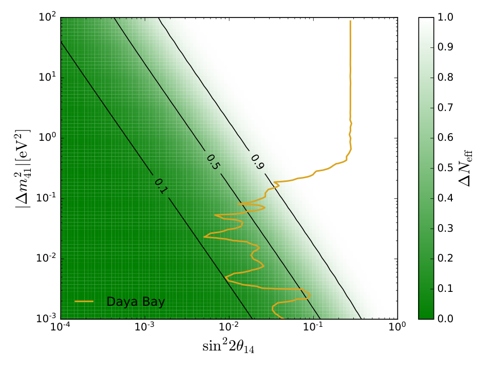
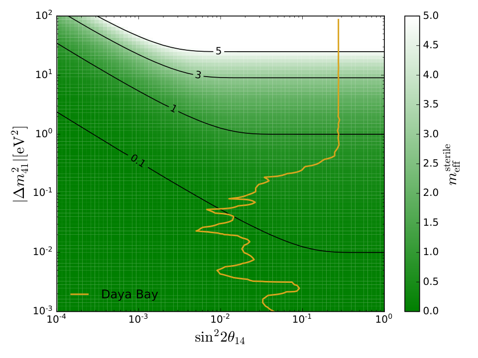
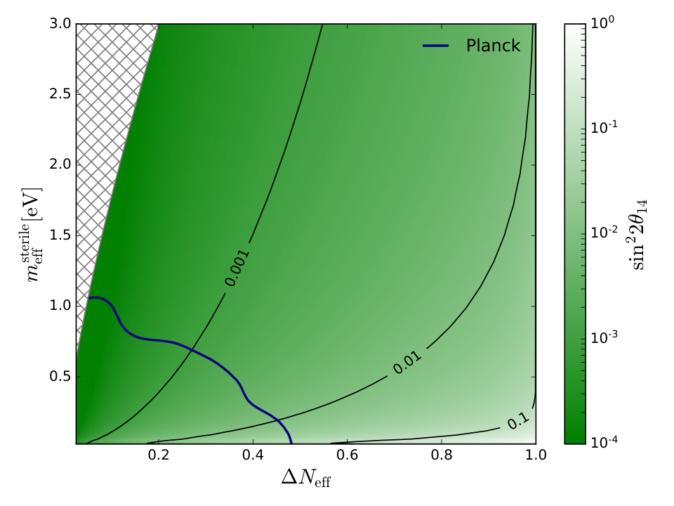
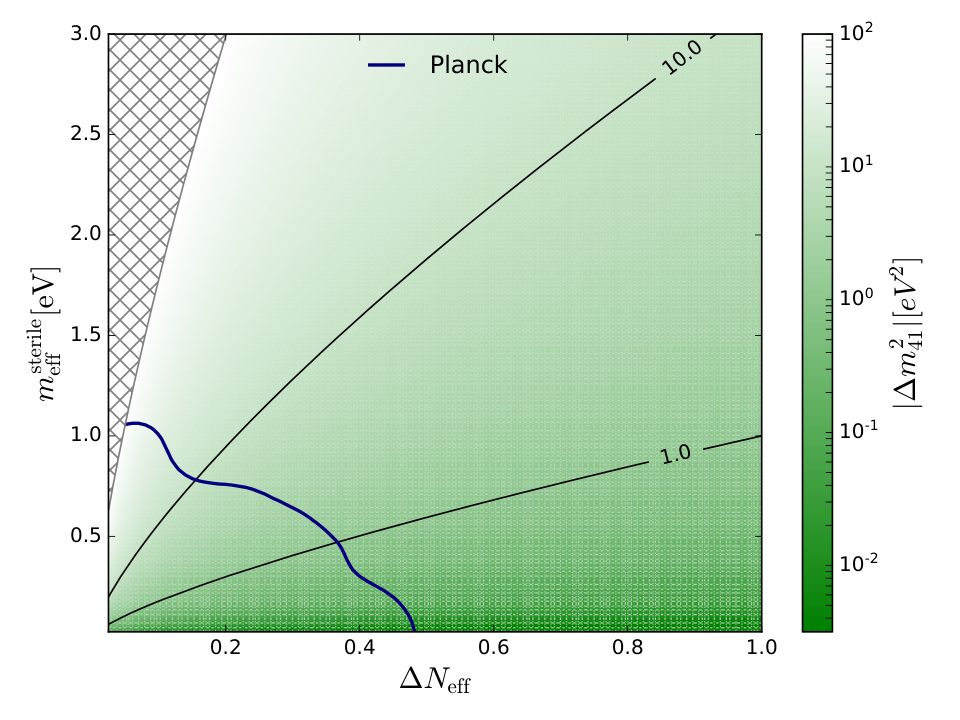
We use LASAGNA to calculate $\Delta N_{\mathrm{eff}}$ for a grid in the oscillation parameter space of $|\Delta m^{2}_{41}|\equiv|m_{4}^{2}-m_{d}^{2}|$ and $\sin^{2}(2\theta_{14})$, as shown in Fig. 1. Equation 8 allows us to express this result for all relevant combinations of $\Delta N_{\mathrm{eff}}$, $m_{\mathrm{eff}}^{\mathrm{sterile}}$, $\sin^{2}(2\theta_{14}),$ and $|\Delta m^{2}_{41}|$ (Figs. 1–1). The figures show that the impact of the sterile state on $\Delta N_{\mathrm{eff}}$ is minimal for small $\sin^{2}(2\theta_{14})$ and $|\Delta m^{2}_{41}|$, increasing to a full extra degree of freedom, $\Delta N_{\mathrm{eff}}=1$, at larger values of the mixing angle and mass splitting. This is related to the amount of thermalisation of the fourth neutrino state in the early universe: a larger mixing angle allows a higher thermalisation rate, and a larger effective sterile neutrino mass (corresponding to a larger mass splitting) increases the temperature at which the thermalisation occurs. More explanation of this can be found in Refs. Steen Hannestad and Tram 2012; Enqvist et al. 1992.

In Fig. 2 we express the Planck exclusion limit in the parameter space $(\sin^{2}(2\theta_{14}),|\Delta m^{2}_{41}|)$ and overlay the limit from Daya Bay, and the allowed regions from Neutrino-4 and the gallium and reactor anomalies. The equivalent contours translated into the cosmological parameter space $(m_{\mathrm{eff}}^{\mathrm{sterile}},\Delta N_{\mathrm{eff}})$ are shown in Fig. 2. In both figures, we show the Planck limit with and without the BAO and CMB lensing data.

The limits obtained using the Planck data with and without the BAO and CMB lensing data are strongly constraining in both parameter spaces in the region above $|\Delta m^{2}_{41}|^{2}\approx 0.1\,\mathrm{eV^{2}}$ and $m_{\mathrm{eff}}^{\mathrm{sterile}}\approx 0.2\,\mathrm{eV}$, and exclude the allowed regions from the Neutrino-4 experiment, and from the gallium and reactor anomalies. The Daya Bay experiment is sensitive to the regions of low $|\Delta m^{2}_{41}|$ and $m_{\mathrm{eff}}^{\mathrm{sterile}}$, where the cosmological data are less constraining.

When considering $\sin^{2}(2\theta_{\mu e})$, both mixing angles $\theta_{14}$ and $\theta_{24}$ must be allowed to be non-zero to allow both $\nu_{e}$ and $\nu_{\mu}$ flavours to mix into the $\nu_{4}$ state, and so we work in the $3+1$ model with one sterile and three active neutrino flavours, albeit setting $\theta_{34}=0$. This model can be solved exactly Gariazzo et al. 2019 but working with the full momentum dependence of the quantum kinetic equations is computationally very intensive. Hence, we use the mean momentum approximation (MMA) following the prescription of Ref. Mirizzi et al. 2012 summarized below.

The neutrino density matrix,

depends on the mixing angles and mass splittings. It can be written as a function of reduced time, $x\equiv m/T$, and reduced momentum, $y\equiv p/T$, where $m$ is an arbitrary mass scale and $T$ is the initial temperature of the thermal, active neutrinos. This matrix is used to calculate $\Delta N_{\mathrm{eff}}$ for any required values of $\theta_{14}$, $\theta_{24}$ and $\Delta m^{2}_{41}$ as

The MMA assumes that the momentum dependence of $\rho(x,y)$ can be factorized out as a Fermi-Dirac distribution, $\rho(x,y)\rightarrow f_{\mathrm{FD}}(y)\rho(x)$. The equations of motion for the neutrino and anti-neutrino density matrices is then written assuming that all neutrinos have the same momentum, $\left<y\right>$.

We solve the resulting differential equations of motion numerically with an implicit Runge-Kutta algorithm of order $5$, RADAU5 Hairer and Wanner 2006, using a publicly available C++ implementation Ashby. To evaluate $\Delta N_{\mathrm{eff}}$, we evolve the density matrix from $T=100\,\mathrm{MeV}$ to $T=1\,\mathrm{MeV}$. To project the cosmological limits onto the $\sin^{2}(2\theta_{\mu e})$ axis, we minimise the value of $\Delta N_{\mathrm{eff}}$ as a function of $\theta_{14}$ and $\theta_{24}$ along a contour of constant $\sin^{2}(2\theta_{\mu e})$; the derived 95% confidence limits therefore assume the maximum possible thermalisation for a given value of $\theta_{\mu e}$. The resulting values of $\Delta N_{\mathrm{eff}}$ as a function of $\Delta m^{2}_{41}$ and $\sin^{2}(2\theta_{\mu e})$ are shown in Fig 3.

In the region $|\Delta m^{2}_{41}|\lesssim|\Delta m^{2}_{31}|$, the mass splitting $\Delta m^{2}_{41}$ is driving neutrino oscillations at wavelengths similar to those driven by the active-neutrino mass splittings. This is referred to as the degenerate region, and in this region the RADAU5 solver slows down drastically due to the stiffness of the problem when degeneracies are crossed. To mitigate this, we increase the tolerance by a factor of 10 after every 100,000 steps of the algorithm, starting from a default tolerance of $10^{-10}$, reaching a maximum tolerance of $10^{-4}$ required for certain parameters to converge quickly.

We evaluate the impact of the MMA by repeating the $\nu_{e}$ disappearance analysis in the $1+1$ model using this approximation. The result of this is shown in Fig 2, illustrating that, under the MMA, the cosmological exclusion contours expressed in the $(\Delta m^{2}_{41},\sin^{2}(2\theta_{14}))$ parameter space become slightly weaker.

In Figure 4, we show the Planck exclusion contours, with and without the BAO and CMB lensing data, in the $(\Delta m^{2}_{41},\sin^{2}(2\theta_{\mu e}))$ parameter space. We compare this to the limits from the Daya Bay/Bugey/MINOS combination, and the allowed regions from the LSND and MiniBooNE $\nu_{e}\rightarrow\nu_{\mu}$ searches. The Planck exclusion region strongly excludes the entirety of the LSND and MiniBooNE allowed regions. The Daya Bay/Bugey/MINOS combined exclusion region is comparable in its exclusion power to that from the Planck data for mass splittings below $\Delta m^{2}_{41}\approx 5\times 10^{-2}\,\mathrm{eV^{2}}$ and becomes more constraining below $\Delta m^{2}_{41}\approx 10^{-3}\,\mathrm{eV^{2}}$.

The discovery of a sterile neutrino would have major implications for the field of particle physics. The presence of both possible observations from neutrino oscillation experiments such as LSND and MiniBooNE, negative results from other oscillation experiments, and negative results from cosmological experiments, have left the field in an ambiguous situation. A particular challenge in drawing conclusions is quantitative comparison of limits from neutrino oscillation data with those from cosmology, due to the different parameter spaces in which measurements from these two sets are expressed.

In this article, we discuss a procedure to convert limits on sterile neutrinos between the $(|\Delta m^{2}_{41}|,\theta_{14},\theta_{24})$ parameter space of neutrino oscillation physics and the $(m^{\mathrm{sterile}}_{\mathrm{eff}},\Delta N_{\mathrm{eff}})$ parameter space of cosmology. We use the LASAGNA software package to solve the quantum kinetic equations of neutrinos in the early universe in a $1+1$ model, allowing us to compare the exclusion regions obtained from Planck data with both allowed regions and exclusion regions from $\nu_{e}$ and $\overline{\nu}_{e}$ disappearance searches. In a $3+1$ model, we use a mean momentum approximation to solve the quantum kinetic equations, allowing us to compare the Planck exclusion with allowed regions and exclusion regions corresponding to $\nu_{\mu}\rightarrow\nu_{e}$ searches. We find that the Planck data strongly excludes the allowed regions from the Neutrino-4, LSND and MiniBooNE experiments, as well as from the gallium and reactor anomalies. Compared to the Daya Bay exclusion region from $\nu_{e}$ disappearance, Planck is much more constraining above $|\Delta m^{2}_{41}|\approx 0.1\,\mathrm{eV^{2}}$ and $m^{\mathrm{sterile}}_{\mathrm{eff}}\approx 0.2\,\mathrm{eV}$, whereas at lower values, Daya Bay provides a more stringent exclusion on $\theta_{14}$. The Planck data provide the strongest exclusion on the $\theta_{\mu e}$ parameter that describes $\nu_{\mu}\rightarrow\nu_{e}$ appearance above $\Delta m^{2}_{41}\approx 5\times 10^{-2}\,\mathrm{eV^{2}}$; below this value, the Daya Bay/Bugey/MINOS combination becomes comparable in terms of its exclusion power.

Experimental and theoretical efforts are ongoing to relieve the tension between positive signals from appearance experiments and the strong exclusions from disappearance measurements and cosmology. Appearance experiments such as MicroBooNE Acciarri et al. 2017 and the SBN programme Antonello et al. 2015 have the potential to rule out or confirm the previous appearance signals. Theoretical work on the cosmological side has to limit thermalisation of the sterile neutrino state in order to maintain $N_{\mathrm{eff}}\approx 3$. Examples include the introduction of new interactions for the sterile neutrino Hannestad et al. 2014; Archidiacono et al. 2015; Saviano et al. 2014; Chu et al. 2015, a large lepton-antilepton asymmetry in the early universe Chu and Cirelli 2006; Foot and Volkas 1995; Saviano et al. 2013b, and the introduction of reheating at low temperatures P. F. de Salas et al. 2015; Kawasaki et al. 2000; Gelmini et al. 2008.