Hardware-Encoding Grid States in a Non-Reciprocal Superconducting Circuit
Abstract
We present a circuit design composed of a non-reciprocal device and Josephson junctions whose ground space is doubly degenerate and the ground states are approximate codewords of the Gottesman-Kitaev-Preskill (GKP) code. We determine the low-energy dynamics of the circuit by working out the equivalence of this system to the problem of a single electron confined in a two-dimensional plane and under the effect of strong magnetic field and of a periodic potential. We find that the circuit is naturally protected against the common noise channels in superconducting circuits, such as charge and flux noise, implying that it can be used for passive quantum error correction. We also propose realistic design parameters for an experimental realization and we describe possible protocols to perform logical one- and two-qubit gates, state preparation and readout.
I Introduction
Building a quantum computer in a physical system is a formidably challenging task because of the inherent fragility of physical quantum bits (qubits). The key idea behind quantum error correction (QEC) Shor 1996; Terhal 2015 is to use logical qubits that can be protected against certain likely errors, thus extending the lifetime of the encoded quantum information and allowing for fault tolerant quantum computation Preskill 1998; Chao and Reichardt 2018.
There are different flavors of QEC codes, that differ in the way in which the logical qubits are constructed. For example, in the toric Kitaev 2003; Dennis et al. 2002, surface Bravyi and Kitaev 1998; Freedman and Meyer 1998; Andersen et al. 2019 and color Bombin and Martin-Delgado 2006 code, the logical qubits are encoded in lattices of physical qubits. To date, the QEC codes that have been most successful in enhancing the lifetime of quantum information have been built from continuous variable (CV) systems Braunstein 1998; Lloyd and Slotine 1998; Lloyd and Braunstein 1999, such as a single microwave cavity mode. Efficient QEC with cat-states and binomial codes has been demonstrated Ofek et al. 2016; Hu et al. 2019. In this work, we focus on a similar CV encoding, proposed by Gottesman, Kitaev and Preskill (GKP) in Ref. Gottesman et al. 2001, where the codewords are shifted grid states and can be protected against sufficiently small translations in phase space. The error correcting properties of the GKP code have been further explored in Ref. Albert et al. 2018, where it was shown that the GKP code outperforms cat and binomial codes when a photon loss channel is considered. Grid states have been successfully prepared and actively stabilized in superconducting cavities by a stroboscopic modulation of interactions Campagne-Ibarcq et al. 2019. Also, passive implementations of these states in superconducting circuits have been proposed with the - qubit Kitaev 2006; Brooks et al. 2013; Dempster et al. 2014; Groszkowski et al. 2018; Gyenis et al. 2019; Di Paolo et al. 2019; Smith et al. 2020 and the dualmon Le et al. 2019.
However, the active implementation of QEC requires complicated protocols where errors are detected and compensated for by applying a recovery operation. In contrast, in passive QEC the protection is a built-in feature of the system’s hardware and it is therefore advantageous in terms of hardware efficiency and scalability. Generally, this is achieved by constructing a system whose two-fold degenerate ground states are the qubit states: errors that bring the system out of the computational space have an associated energy penalty and so the system will automatically relax back into the computational space Kitaev 2003; Douçot and Ioffe 2012; Bravyi et al. 2010.
An example of an implementation of the GKP code is a single electron confined in a two-dimensional plane within a periodic potential and a high perpendicular magnetic field Onsager 1952; Harper 1955; Azbel 1964; Zak 1964; Zak 1967; Zak 1968; Zak 1970; Rauh et al. 1974; Rauh 1974; Rauh 1975; Hofstadter 1976; Hsu and Falicov 1976; Wannier 1978; Springsguth et al. 1997. The magnetic field restricts the dynamics of the electron to the lowest Landau level (LLL), so that the position operators in orthogonal directions do not commute. The contribution of the periodic potential to the Hamiltonian reduces to a sum of displacement operators, which are the stabilizers of the GKP code.
Although this system is useful for a theoretical understanding of the code, it is very unpractical to implement. The magnetic field required for it to work is exactly with the area of the unit cell in space and the magnetic flux quantum . In realistic crystals, this condition implies that the magnetic field needs to be unrealistically large, about . Moiré patterns in twisted bilayer graphene can be used to reduce this value by a few orders of magnitude due to their large unit cell Dean et al. 2013. Even if such a regime were possible to achieve, the external magnetic field would still require an extremely precise fine-tuning and the electron density would still have to be decreased to the unfeasible value of a single free electron in the crystal.
Here, we propose instead a different implementation of the GKP code, which does not suffer from any of these issues. We consider a superconducting circuit composed of two Josephson junctions coupled by a classic, lossless, linear non-reciprocal circuit element, the gyrator Tellegen 1948. The circuit is shown in Fig. 1.
The non-reciprocity of the gyrator breaks time-reversal symmetry and its contribution to the dynamics of the circuit is akin to that of a uniform, perpendicular magnetic field in an electronic system. In our circuit, the condition on the strength of the magnetic field reduces to the requirement on the gyration conductance being precisely twice the conductance quantum, i.e. .
While unrealistic for conventional gyrators Hogan 1952; Hogan 1953; Rosenthal et al. 2017; Chapman et al. 2017; Lecocq et al. 2017; Barzanjeh et al. 2017, this value of can be easily reached in quantum Hall effect (QHE) devices Viola and DiVincenzo 2014; Bosco et al. 2017; Bosco and DiVincenzo 2017; Bosco et al. 2019; Mahoney et al. 2017a, in which a precise fine-tuning of the device parameters is unnecessary due to the quantization of the off-diagonal conductivity. In addition, although conventional QHE devices Mahoney et al. 2017a require a high magnetic field to operate, making them unpractical to couple to superconducting devices, we note that state-of-the-art quantum anomalous Hall effect materials still present an extremely precise conductivity quantization and low losses Bestwick et al. 2015 and can be used to implement non-reciprocal electrical network elements that can operate at zero magnetic field Mahoney et al. 2017b.
We show that our construction is insensitive to common types of noise. We discuss possible ideas of how logical one-qubit as well as two-qubit Clifford gates can be implemented by applying currents and using tunable inductances. We show that the ground state of our system is an eigenstate of the Hadamard gate. Consequently, our system is suitable for universal quantum computation Gottesman et al. 2001; Bravyi and Kitaev 2005; Yamasaki et al. 2019.
The paper is organized as follows: In Sec. II we review a few key concepts of hardware-encoding GKP states and we introduce the Hamiltonian whose two-fold degenerate ground space is spanned by the GKP codewords. In Sec. III we show how this Hamiltonian can be derived from the low-energy description of a single electron in a high magnetic field and a periodic potential. The dynamics of this system is equivalent to that of a gyrator connected to two Josephson junctions but the solid-state jargon more easily reveals the intimate relation to Hoftstader’s butterfly Hofstadter 1976; Springsguth et al. 1997: the GKP states are obtained at a specific point in the butterfly. In Sec. IV we study the effect of an additional parabolic confinement potential, which in the circuit model consists of the addition of inductances in parallel to the Josephson junctions. For this setting, the ground space of the resulting Hamiltonian is two-fold degenerate up to an exponentially small gap and the eigenstates of the system resemble superpositions of normalizable, approximate GKP codewords Gottesman et al. 2001. In Sec. V we highlight the connection between the one-dimensional GKP grid states and the two-dimensional ground space wave functions of the electronic system’s Hamiltonian projected onto the lowest Landau level. In Sec. VI we work out in detail the equivalence to the non-reciprocal superconducting circuit model and we propose realistic design parameters for an experimental realization of the system. We also discuss possible realizations of logical gates by using current sources and tunable inductances and we present ideas for state preparation and readout. We provide an analysis of the protection against common noise sources, such as flux and charge noise. Finally, in Sec. VII we summarize our results and give an outlook on further work.
II The GKP code for passive QEC
The GKP code is a CV quantum error correcting code Braunstein 1998; Lloyd and Slotine 1998; Lloyd and Braunstein 1999 introduced in Ref. Gottesman et al. 2001. In contrast to the standard approach to quantum error correction, which assumes physical qubits as fundamental noisy elements, in CV quantum error correction the idea is to encode a two-level (or -level more generally) system in the infinite-dimensional Hilbert space of an one-dimensional particle characterized by dimensionless canonical quadrature operators and satisfying . The GKP code can be described within the stabilizer formalism for CV systems. The role of the Pauli group is played by the Weyl-Heisenberg group , i.e. the group of displacement operators Weedbrook et al. 2012; Gerry and Knight 2005
| (1) |
with the annihilation operator . In this framework the GKP code is the -dimensional subspace stabilized by a subgroup of with group generators
| (2) |
and . The logical Pauli operators and are given by
| (3) |
This choice of logical operators fixes the following (unnormalizable) codewords
| (4a) | ||||
| (4b) | ||||
that are grid states, each describing a comb of equidistant -peaks in the -basis. These combs have a period of and are shifted with respect to each other by .
Given a density matrix describing the state of an one-dimensional CV quantum system, one can expand a generic quantum operation in terms of displacement operators as Gottesman et al. 2001
| (5) |
with being a scalar function. If the function has support only on a domain in which is either in the stabilizer group or does not commute with the stabilizers and in Eq. (2), then the GKP code can correct against these kinds of errors, provided that shifts in position and momentum obey
| (6) |
In this case, the error syndromes are unique. Otherwise, logical errors will be made.
The main idea behind passive, stabilizer error correction is to construct a Hamiltonian that has the code subspace as the low energy subspace. For the GKP code, this Hamiltonian is easily obtained as Gottesman et al. 2001
| (7) |
with a constant with the unit of energy. Because the code subspace is stabilized by the two cosines it has energy .
We remark that passive, stabilizer error correction for CV systems is rather different than in systems based on a large set of physical qubits, such as the toric, surface or color code Kitaev 2003; Dennis et al. 2002; Bravyi and Kitaev 1998; Freedman and Meyer 1998; Bombin and Martin-Delgado 2006. In fact, the Hamiltonian in Eq. (7) is gapless, with a continuous spectrum ranging from to . Also, because the Weyl-Heisenberg group is a continuous group, in contrast to the discrete Pauli group, the eigenstates of are unnormalizable and formally out of the Hilbert space of any physical system. As a consequence, the usual perturbation theory argument Kitaev 2003; Bravyi et al. 2010 which claims that local perturbations of the Hamiltonian give rise to small variations of the energy levels is not applicable here. As pointed out in Ref. Douçot and Ioffe 2012, the argument can be restored in approximated versions of Eq. (7), where the eigenstates are normalized and confined, leading to a discrete spectrum. The particular way in which is approximated modifies the properties of the degenerate ground space, but generally its eigenstates remain with disjoint support. This idea of passive protection is similar to the one behind the - qubit Kitaev 2006; Brooks et al. 2013; Dempster et al. 2014; Groszkowski et al. 2018; Gyenis et al. 2019; Di Paolo et al. 2019; Smith et al. 2020.
III Crystal Electron in Magnetic Field
We discuss how the code Hamiltonian in Eq. (7) can emerge from the consideration of the well-known situation of a single electron confined to a two-dimensional plane in a strong perpendicular uniform magnetic field Onsager 1952; Harper 1955; Azbel 1964; Zak 1964; Zak 1967; Zak 1968; Zak 1970; Rauh et al. 1974; Rauh 1974; Rauh 1975; Hofstadter 1976; Hsu and Falicov 1976; Wannier 1978; Springsguth et al. 1997. The effect of a periodic potential on the electron’s motion has been extensively studied because of the fractal nature of the energy bands Hofstadter 1976 and their non-trivial topology Thouless et al. 1982. In this section, we want to clarify under what conditions the ground states of the system are GKP states. We focus on the Hamiltonian
| (8) |
where the two-dimensional positions and momenta satisfy canonical commutation relations , for , and . We consider a crystal potential of the form
| (9) |
which corresponds to the first Fourier mode of any periodic potential on a square lattice of size in the -plane. Although both the crystal potential and the uniform magnetic field are periodic in the - and -direction, the Hamiltonian is not, because the discrete translation symmetry is broken in at least one direction by the vector potential . As a result, does not simultaneously commute with both the canonical unitary translation operators and , defined as
| (10) |
It follows that and cannot have common eigenstates, as the usual formulation of Bloch’s theorem dictates. To find a set of translations which do commute with the Hamiltonian, we work with the dynamical momenta Prange and Girvin 1990; Douçot and Pasquier 2005; Tong 2016; Girvin and Yang 2019
| (11) |
and the guiding center variables
| (12) |
with the cyclotron frequency . These operators are gauge-invariant (in contrast to the canonical momenta ) and satisfy the commutation relations
| (13) |
for and the magnetic length . Physically, the dynamical momenta are related to the cyclotron motion of an electron around its center of mass, which in turn is parametrized by the guiding center coordinates.
We can impose boundary conditions by requiring the wave function to be quasi-periodic in . To this end, we make use of the unitary magnetic translation operators (MTOs) Zak 1964; Girvin and Yang 2019; Brown 1964; Fischbeck 1963 11 1 In the -representation, the MTOs differ from the conventional translation operators, as defined in Eq. (10), by an additional -dependent complex phase, originating from the gauge of the vector potential .
| (14) |
which shift the guiding center variables by , i.e.
| (15) |
It is straightforward to show that the MTOs and do commute with the Hamiltonian in Eq. (8). However, because of the non-commutativity of and in Eq. (12), magnetic translations in different directions do not generally commute. An electron moving along a closed path accumulates an Aharonov-Bohm phase Aharonov and Bohm 1959 proportional to the magnetic flux threaded by the loop and so
| (16) |
with the (non-superconducting) flux quantum . Consequently, MTOs in orthogonal directions commute only when an integer number of flux quanta is threaded through the loop defined by the MTOs. Note that with an appropriate rescaling, the MTOs defined in Eq. (14) correspond to the displacement operators similar to the ones defined in Eq. (1).
In the following, we restrict to rational fluxes Hofstadter 1976, where the magnetic flux enclosed in a unit cell of size is a rational multiple of the flux quantum, i.e.
| (17) |
with coprime natural numbers and . In this case, we consider an enlarged, magnetic unit cell of size , which contains flux quanta, such that the MTOs and commute with the Hamiltonian in Eq. (8) and with each other 22 2 We remark that the direction of the enlargement is arbitrary.. As a result, we consider the magnetic Bloch states satisfying
| (18a) | ||||
| (18b) | ||||
where is the crystal momentum defined in the rectangular Brillouin zone
| (19) |
The states are sometimes referred to as Zak states Zak 1970; Zak 1967; Zak 1968.
Introducing the Landau level ladder operators
| (20) |
satisfying the bosonic commutation relation , the Hamiltonian in Eq. (8) can be rewritten as
| (21) |
with the cyclotron frequency and the unitary displacement operator acting on the subspace of the dynamical momenta. A convenient basis to numerically analyze the low energy spectrum of this Hamiltonian are the product states satisfying
| (22) |
and
| (23a) | ||||
| (23b) | ||||
| (23c) | ||||
with , see Appendix A. Note that in the absence of the potential (), the states diagonalize the Hamiltonian, leading to the -fold degenerate Landau level spectrum . Expressed in the -representation, the quasi-periodic wave functions were introduced by Haldane and Rezayi in Ref. (Haldane and Rezayi 1985), see also Sec. V.
The crystal potential couples states with different Landau level occupation number and with different guiding center quantum number . Consequently, the -fold degeneracy is lifted and, for a moderately weak crystal potential, each Landau level splits into subbands with finite broadening and -fold degeneracy Rauh 1974; Rauh 1975; Rauh et al. 1974, see Fig. 2, in which the two lowest split Landau levels are shown. More details on the general solution of the Hamiltonian in Eq. (21) can be found in Appendix B.1.
In this paper, we are interested in the weak Landau level coupling limit , where the dynamics of states within each Landau level can be taken to be independent from the others. This limit will be analyzed in the following.
III.1 GKP Qubit in the LLL Projection
When the coupling between the Landau levels is weak, an effective low-energy Hamiltonian acting on a single Landau level can be obtained by a Schrieffer-Wolff transformation Winkler 2003; Bravyi et al. 2011. In particular, to the lowest order and considering only the LLL 33 3 The treatment of higher Landau levels is similar and straightforward., we obtain from Eq. (21) the effective Hamiltonian (up to an unimportant constant)
| (24) |
where . Although formally this effective Hamiltonian is valid only when , numerics shows that the approximation holds up well to relatively high values of , see Sec. IV.2 where we discuss in more detail the validity of the LLL projection.
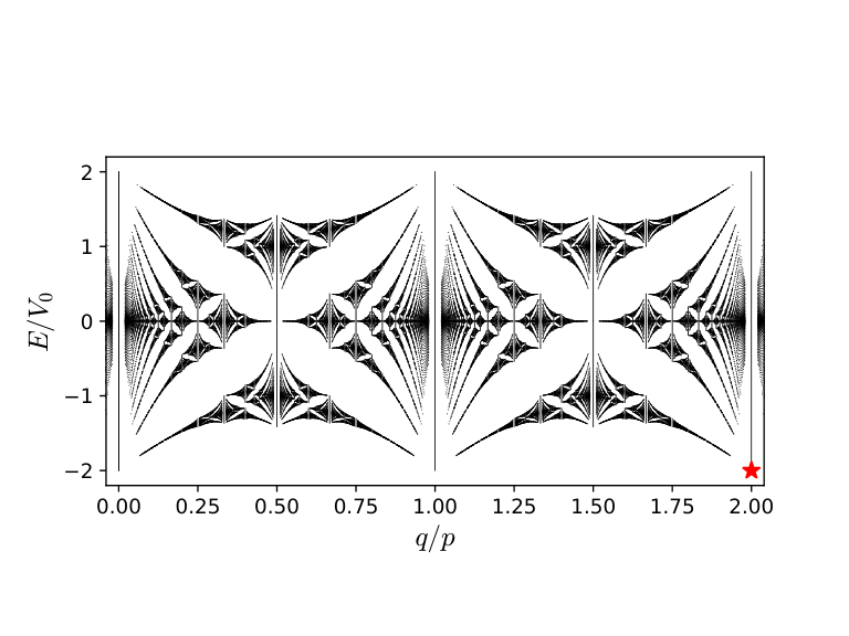
In the limit of weak Landau level coupling, the eigen equation associated with is the Harper equation Harper 1955; Springsguth et al. 1997; Azbel 1964; Hsu and Falicov 1976; Andrei Bernevig and Hughes 2013, which is a special case of the almost Mathieu equation (Bellissard and Simon 1982; Avila and Jitomirskaya 2009; Avila 2008). In particular, the Harper equation is a finite-difference equation, resulting in an energy spectrum in form of the Hofstadter butterfly Hofstadter 1976, shown in Fig. 3.
We point out that this spectrum has bands that are -fold degenerate. In fact, states connected by the application of with are orthogonal but have the same energy, see Appendix A. Note that this result is in contrast to the original tight-binding result of Hofstadter Hofstadter 1976, where different Landau levels are strongly coupled and where there are bands that are -fold degenerate Andrei Bernevig and Hughes 2013. For this reason, in the original work the Hofstadter butterfly is obtained by plotting the spectrum as a function of instead of Hofstadter 1976.
Importantly, by introducing the dimensionless variables
| (25) |
satisfying the canonical commutation relation , we can rewrite as
| (26) |
Comparing with Eq. (7), we observe that corresponds to the GKP Hamiltonian when . This system is therefore suitable for passively encoding the GKP codewords, which are given in Eq. (4). Note that for , the previous rescaling of the guiding center variables becomes equal, and so the code can correct equal shifts on and .
Furthermore, for , the MTOs defining the states in Eq. (18) are related to the stabilizers and logical operators of the GKP code as
| (27) |
Since the GKP codewords are the eigenstates of with minimal eigenenergy, we can identify the code space with a specific point in Hofstadter’s butterfly (see the red star in Fig. 3). In particular, the code space is spanned by the eigenstates obtained for and . These states correspond to the logical codewords introduced in Eq. (4). The eigenfunctions of the full system within the LLL projection will be analyzed in Sec. V.
At this point, we would like to highlight the main difference between our approach and the original proposal by GKP Gottesman et al. 2001. GKP proposed to use the LLL projection at the rational flux without the crystal potential (). A qudit can be encoded by focusing on the -fold degenerate ground space obtained at vanishing Bloch momentum (), and one can take this qudit to construct different shift resistant quantum codes. In contrast, for the rational flux , by including the crystal potential and using states with different Bloch momenta, here we encode a qubit in a real CV system.
IV Additional parabolic confinement
Because the GKP codewords in Eq. (4) are not normalizable, they are mathematical objects that are not physically realizable. Furthermore, the continuous spectrum of is problematic for the implementation of the GKP code in realistic systems, since noise or temperature would affect the states Douçot and Ioffe 2012. For these reasons, we consider an additional parabolic potential in the Hamiltonian in Eq. (8). This potential renders the spectrum discrete and the states normalizable. We show that the eigenstates of this modified Hamiltonian are related to the approximate grid states introduced in the original work by GKP Gottesman et al. 2001.
For simplicity, we choose the parabolic confining potential to be isotropic and so the Hamiltonian is
| (28) |
with
| (29) |
Because does not preserve the discrete translational symmetry defined by , we cannot impose the magnetic Bloch conditions in Eq. (18). In this case, we require instead that the wave functions vanish at infinity.
We now briefly summarize the main findings of a numerical analysis of the eigensystem of the Hamiltonian in Eq. (28) (see Appendix B.2 for details). In particular, we focus on the case , see Eq. (17), which in the LLL projection leads to ideal GKP states in the absence of the parabolic confinement potential. As in the previous section, we construct and analyze a low energy theory of the system, valid in the weak Landau level coupling limit.
IV.1 Numerical Results
When a confinement potential is included, the two-fold degeneracy of the ground space is lifted and an energy gap opens between the degenerate ground states of in Eq. (26). This energy gap, however, is exponentially small in , and so the ground state and the first excited state remain quasi-degenerate when is small enough. To illustrate this point, in Fig. 4, we show the lowest ten eigenenergies of the Hamiltonian in Eq. (28) as functions of the confinement strength for a rather large value of . Recall that denotes the amplitude of in Eq. (9). We observe that the energy gap between the ground state and first excited state is negligibly small up to confinements of , and that it nicely fits an exponential scaling , with a positive constant prefactor . In addition, the spectrum is now discrete and higher excited states are gapped from the two-fold quasi-degenerate ground space.
As mentioned in Sec. II, the discreteness of the spectrum then allows one to use a perturbative argument which states that local perturbations do not considerably alter the spectrum of the Hamiltonian.
Because we are interested in the weak Landau level coupling limit, we analyze the effect of higher Landau levels on the low energy eigenstates numerically. In Fig. 5 we show how the expectation value of the LLL projector in the ground state of the Hamiltonian in Eq. (28) varies as a function of the confinement potential for fixed values of . We observe that the higher Landau levels have a negligible effect for a wide range of parameters, giving an error below for rather large values of both and , and, consequently, justifying even in this case a projection onto the LLL. In particular, at the values and , which are the relevant parameters for the circuit model presented in Sec. VI, we find , see the green circle in Fig. 5.
The effective Hamiltonian of the system in this limit is analyzed in the next section.
IV.2 Approximate Grid States in the LLL Projection
In analogy to Sec. III.1, here we find an effective Hamiltonian that captures the behavior of the system in the weak Landau level coupling limit. By projecting Eq. (28) onto the LLL and considering , we obtain
| (30) |
where and the canonical position and momentum are defined by Eq. (25).
Importantly, the parabolic potential in Eq. (29) reduces to the harmonic oscillator Hamiltonian with frequency after the LLL projection, and breaks the periodicity of both and . However, note that the confinement potential preserves the four-fold rotational symmetry in and . Because a rotation in the -plane reduces to a Fourier transform, which maps and , when projected onto the LLL, the Hamiltonian in Eq. (30) is invariant under the exchange of and and its eigenstates are also eigenstates of the Fourier transform. More detailed explanations of this symmetry and correspondence are given in Appendices B.2 and E.
In particular, the two quasi-degenerate low-energy eigenfunctions (ground state) and (first excited state), shown in Fig. 6, are even and odd eigenfunctions of the Fourier transform with eigenvalues , respectively. These states are well approximated by the linear combinations
| (31a) | ||||
| (31b) | ||||
of the approximate grid states
| (32a) | ||||
| (32b) | ||||
that are shown in Fig. 7. Explicitly, the squeezing parameter is given by
| (33) |
These approximate grid states are obtained by a convolution of the ideal grid states in Eq. (4) with a narrow Gaussian of width and a multiplication with a wide Gaussian of width . This inverse relation is a consequence of the invariance of the Hamiltonian with respect to the Fourier transform and it also reflects the fact that the GKP code corrects equal errors in the - and -variable.
When the confinement frequency is decreased, the width of the individual Gaussian peaks of the approximate grid states in Eq. (32) decreases, while the broadening of the envelope function increases, eventually recovering the ideal grid states in Eq. (4) when .
The derivation of Eqs. (31) - (33) is based on a nested application of the envelope function approximation Girvin and Yang 2019; Kittel 1987; Rossi 2011 discussed in Appendix C. Note that, when the parameter is rather small, as we are considering here, the states and are orthonormal up to an exponentially small correction scaling as . Consequently, they form an appropriate computational basis for the quasi-degenerate ground space of .
The angle which appears in the linear combination in Eq. (31) can be understood by considering that in the basis , the Fourier transform approximately equals the Hadamard gate Gottesman et al. 2001
| (34) |
whose even and odd eigenfunctions are and , respectively 44
4
On the Bloch sphere, the Hadamard gate corresponds to a -rotation around the axis defined by .. These states are magic states which combined with Clifford operations achieve universal quantum computation Gottesman et al. 2001; Bravyi and Kitaev 2005; Yamasaki et al. 2019; Baragiola et al. 2019.
We remark that an alternative low-energy description of the Hamiltonian in Eq. (28) which relies on the introduction of the eigenbasis of the quadratic part of the Hamiltonian is possible. This basis is known as Fock-Darwin basis Fock 1928; Darwin 1931. In the weak Landau level coupling limit, the results obtained with this approach are equivalent to the ones shown here.
V Eigenfunctions of the two-dimensional problem
So far, we described eigenfunctions of an one-dimensional Hamiltonian obtained by projecting a two-dimensional Hamiltonian onto the LLL. Here, we establish the connection between the eigenfunctions of these two Hamiltonians. In the weak Landau level coupling regime, which we considered in the previous sections, the wave function of the two-dimensional system is the coherent state representation of the wave function of the one-dimensional system.
In the following, we begin by considering the ideal case discussed in Sec. III and then we straightforwardly generalize our result to include the parabolic confinement potential as introduced in Sec. IV.
In the weak Landau level coupling limit, the low-energy eigenstates of the Hamiltonian in Eq. (21) are well approximated by the product state
| (35) |
where denotes the LLL and is an eigenstate of the projected Hamiltonian in Eq. (26). From Eq. (35), it follows that the wave function in the original coordinates and the one-dimensional wave function are related by the unitary integral transform
| (36) |
where is a gauge-dependent integration kernel. As derived in Appendix D, in the symmetric gauge, i.e. , we obtain
| (37) |
To simplify the notation, in this section, we work in magnetic units and we rescale all the lengths by the magnetic length .
Note that, up to a gauge phase , the integration kernel is the complex conjugate of the wave function (in -representation) of a coherent state with average position and momentum and , respectively. Consequently, as long as the matrix elements between different Landau levels are small and the approximate factorization in Eq. (35) is valid, the low-energy two-dimensional eigenfunctions of the Hamiltonian in Eq. (21) are the coherent state representations of the eigenfunctions of the projected Hamiltonian in Eq. (26) Chruściński and Młodawski 2005. It follows that the absolute value squared is the non-negative Husimi representation Walls and Milburn 2007; Gerry and Knight 2005; Subramanyan and Vishveshwara 2019 associated with . Note also that the integral transform in Eq. (36) is invertible and preserves orthonormality.
Let us consider now the LLL non-normalizable eigenfunction
| (38) |
of the effective Hamiltonian in Eq. (26), satisfying the quasi-periodic boundary conditions defined by Eq. (23) with and . Because of the choice , the length (in magnetic units) reduces to , see Eq. (17). The wave function of the two-dimensional system, obtained via the integral transform in Eq. (36), is
| (39) |
with the generalized elliptic theta function
| (40) |
Note that the absolute value of the wave function in Eq. (39) is periodic in both and , i.e. . Similar two-dimensional functions satisfying quasi-periodic boundary conditions were introduced by Haldane and Rezayi Haldane and Rezayi 1985 as a basis to describe the problem of an electron confined to the surface of a torus and under the effect of a perpendicular magnetic field.
The two-fold degenerate ground space of the effective Hamiltonian in Eq. (26) is spanned by the logical codewords in Eq. (4), which are obtained from Eq. (38) by considering and , respectively. As discussed in Sec. IV.2 and in Appendix E, -rotations in the -plane correspond to a Fourier transform after the LLL projection. Consequently, because in the basis and a Fourier transform is equivalent to a Hadamard gate Gottesman et al. 2001 (see Sec. IV.2), to construct four-fold rotational symmetric wave functions in the two-dimensional plane, we consider the linear combinations 55 5 Note that Eq. (41) is exact because the ideal GKP states are considered. In contrast, in Sec. IV.2 we considered approximate grid states.
| (41a) | ||||
| (41b) | ||||
These functions are even (odd) under Fourier transform and so the corresponding two-dimensional wave functions are even (odd) under a -rotation around the origin . The absolute values of the functions are shown in Fig. 8. We observe that the absolute values are periodic with period in both - and -direction. Also, we find that these states are related to each other by
| (42) |
and so the absolute values of the two wave functions are simply obtained by a shift of in the - and -direction.


As long as the Landau level coupling remains weak, Eq. (36) is appropriate to describe also the system discussed in Sec. IV, where an additional parabolic potential is included. In particular, we find that the approximate grid states given in Eq. (32) transform into
| (43) |
with and being defined in Eq. (33). The low-energy eigenstates of the Hamiltonian in Eq. (28) are related to these basis states by Eq. (31), and their absolute values obtained for are shown in Fig. 9.


Comparing Figs. 8 and 9, we observe that the parabolic potential introduces a Gaussian decay roughly of the order of the wave functions in both - and -direction and also it distorts the arguments of the theta functions with corrections of order . Of course, the absolute values of the wave functions in Fig. 8 are recovered by taking the limit .
VI GKP Hamiltonian in a non-reciprocal superconducting circuit
Here, we propose a possible experimental realization of the Hamiltonian in Eq. (28) based on a combination of state-of-the-art non-reciprocal superconducting circuits. We consider here the circuit shown in Fig. 10.
The device consists of two fluxonia coupled by a gyrator. The fluxonium is a well-known superconducting circuit comprising a Josephson junction with Josephson energy in parallel with a capacitance and an inductance Manucharyan et al. 2009; Nguyen et al. 2019 66 6 Strictly speaking, this superconducting circuit is only called to be a fluxonium if it is operated in the parameter regime and . However, regardless of this choice of parameters and for the sake of convenience, we refer to the circuit as fluxonium.. The crucial difference of our design from more conventional superconducting qubit architectures is the non-reciprocity that comes from the gyrator Tellegen 1948.
A gyrator is a two-port linear device that relates incoming currents and voltages according to
| (44) |
where is the frequency-independent gyration conductance. Because it is characterized by an anti-symmetric admittance matrix , this device is non-reciprocal and breaks the time-reversal symmetry of the circuit.
While the typical implementations of these devices are quite bulky Hogan 1952; Hogan 1953, there are also recent realizations of miniaturized on-chip non-reciprocal devices based on actively pumped systems Rosenthal et al. 2017; Chapman et al. 2017; Lecocq et al. 2017; Barzanjeh et al. 2017 or based on the quantum (anomalous) Hall effect Mahoney et al. 2017b; Mahoney et al. 2017a. Although our model is independent of the specific realization of the gyrator, the latter devices are advantageous in this context because they are passive and they rely on quantized excitations with a long lifetime that can be well-described by the theory of circuit quantum electrodynamics (cQED) Vool and Devoret 2017; Girvin 2014. A further advantage will be the value of .
To describe the system with circuit quantization theory, we introduce the node fluxes . Using Kirchoff’s laws, the following contribution to the Lagrangian Rymarz 2018; Duinker 1959
| (45) |
correctly reproduces the defining property of the gyrator in Eq. (44) when two general classical networks are attached to it. Importantly, note that (in the style of an electronic system) Eq. (45) is similar to the effect of a homogeneous magnetic field of strength passing through the -plane. More details on circuit quantization of non-reciprocal devices can be found in Refs. Rymarz 2018; Parra-Rodriguez et al. 2019.
For now, we neglect the effect of magnetic fluxes threading the superconducting loops and we set . Combining conventional circuit QED with Eq. (45), we find the Hamiltonian of the circuit in Fig. 10 to be
| (46) |
We then impose the canonical commutation relation . Here, are the charges on the ’th capacitor. Note that the superconducting flux quantum differs from the flux quantum used in the previous sections by a factor . For simplicity, we assumed here that the two fluxonia coupled to the gyrator are identical. We do not expect small anisotropies to drastically alter the results described in this section.
The Hamiltonian in Eq. (46) describing our circuit has the same structure as the Hamiltonian of a confined crystal electron in a magnetic field in Eq. (28) and discussed in detail in Sec. IV. The variables that play equivalent roles in the two cases are given in Table 1.
| Crystal electron | |||||||
|---|---|---|---|---|---|---|---|
| Circuit |
In particular, the gyration conductance acts as a magnetic field and the characteristic frequency of the LC circuit acts as the harmonic confinement . For later convenience, we also introduce the charging energy and the inductive energy .
As shown in Sec. III, the number of flux quanta threading one unit cell is of fundamental importance for realizing GKP states. In our circuit, Eq. (17) becomes
| (47) |
where we introduced the superconducting conductance quantum . In order to obtain GKP states, we require and, accordingly, we require the gyration conductance to be precisely
| (48) |
We remark again that while this value of is unrealistic for superconducting based gyrators, it can be easily reached using quantum (anomalous) Hall effect devices, where the characteristic impedance is Viola and DiVincenzo 2014; Bosco et al. 2017; Bosco and DiVincenzo 2017; Bosco et al. 2019; Mahoney et al. 2017a; Bestwick et al. 2015; Mahoney et al. 2017b, with being the Landau level filling factor. The robust quantization of the Hall conductivity in these materials also guarantees that the value of remains precisely fixed for a wide range of design parameters, hence improving the reproducibility of the gyrator.
To reach low values of the harmonic confinement frequency , we expect that the novel hyperinductances Pechenezhskiy et al. 2019, the kinetic inductances based on granular aluminum Maleeva et al. 2018; Grünhaupt et al. 2019 or thin Nb nanowires Niepce et al. 2019 will be suited. Also, the Josephson junctions should work in the charge regime , which guarantees a weak Landau level coupling. In Table 2, we list parameter values that are experimentally achievable in state-of-the-art superconducting circuits and that can be used to design GKP qubits. The resulting, relevant energy ratios which need to be small are and . For the parameter defining the widths of the approximate grid states (see Sec. IV.2), we obtain .
| Parameter | |
|---|---|
We emphasize that our circuit encodes the approximate grid states in a subsystem (to be precise, in the LLL) whose dynamics is effectively described by the approximate GKP Hamiltonian in Eq. (30). For this reason, the codewords are passively protected Douçot and Ioffe 2012, and so, in contrast to current efforts to encode grid states in superconducting cavities Campagne-Ibarcq et al. 2019, they do not require permanent active stabilization Douçot and Ioffe 2012.
We also point out that there is a different proposal for a superconducting circuit implementing grid states in a doubly non-linear qubit (the dualmon) Le et al. 2019, which involves a Josephson junction and a quantum phase-slip wire. However, in contrast to our proposal, its dynamics is not described within a Landau level projection and also the GKP codewords are not the lowest-lying eigenstates of the resulting Hamiltonian Le et al. 2019.
So far, we neglected the effect of potential external magnetic fluxes threading the superconducting loops in the circuit shown in Fig. 10. Also, no external voltage or current sources have been attached to it. In the following, we show how these additional degrees of freedom can be used to perform single- and two-qubit gates and for state preparation and qubit read out. Because of the assumed symmetry between the fluxonia, the effective Hamiltonian is symmetric in and and so quantum operations can be performed in the logical or basis depending on which port of the gyrator the sources are applied to.
VI.1 Logical and gates
We now turn our attention to the implementation of logical gates in our system by focusing on the single-qubit and gates defined in Eq. (3). For the sake of clarity, we will carry out the analysis for the case without harmonic confinement potential, i.e. without inductances in the superconducting circuit. The same procedures also work for the complete circuit in Fig. 10 when the ratios and are sufficiently small, yielding approximate logical gates.
In our analysis, we demand that the system is operated in the relevant case of weak Landau level coupling as discussed in Sec. III.1. The logical operators and can be implemented using current sources shunting either of the ports of the gyrator. The circuit implementing the gate is depicted in Fig. 11.
The Hamiltonian of this circuit can be written as
| (49) |
where in analogy with the electronic case, see Eqs. (11) and (12), we defined the dynamical momenta , and the guiding centers , . The current source appears in the Hamiltonian in the term . Note that in the electronic analogy, the current source acts as a homogeneous and time-dependent in-plane electric field, whose direction depends on the port the generator is connected to. We expect that if the current source does not contain frequencies close to , it will not cause transitions between Landau levels. Hence, we can project onto the LLL and obtain (dropping constant shifts in energy)
| (50) |
where we immediately performed the variable rescaling in Eq. (25). Also, we used the definition of the GKP Hamiltonian in Eq. (7) to identify .
Now, we consider the following scenario. At time , the state is assumed to be in a generic superposition of the ideal GKP codewords given in Eq. (4). We assume a constant current source . In this case, the time evolution operator associated with in Eq. (50) reduces to . In order to understand the effect of on we use the Zassenhaus formula Suzuki 1977
| (51) |
with and . Since all the commutators in the Zassenhaus formula have the GKP states as degenerate eigenstates, e.g.
| (52) |
one can show that
| (53) |
where we factorized the irrelevant phase factor . Thus, after a time
| (54) |
a logical gate is applied to , up to an overall phase. Ideally, after a time , the current source must be switched off.
As already mentioned, because of the exchange symmetry of our circuit, it is straightforward to convert between the logical and basis by simply changing the port of the gyrator where the current source is applied and using the same protocol.
VI.2 Noise Sensitivity
We provide a first analysis of the noise sensitivity of our qubit to typical noise sources, such as flux and charge noise. We start our discussion by analyzing charge noise. In the circuit in Fig. 10, charge noise can be modeled by capacitively coupling random voltage sources to the ports of the gyrator. This modifications change the kinetic term in the Hamiltonian in Eq. (46) as , where is a vector containing the random charges on the capacitors connected to the voltage sources on either side of the circuit. The eigenspectrum is insensitive to static gate charges since they can be gauged away by a unitary transformation, as for the fluxonium qubit Manucharyan et al. 2009; Manucharyan 2012. Moreover, charge noise couples to the dynamical momenta , and, as a consequence, it has only a small effect on the guiding center variables in which our states are encoded. From these arguments we conclude that charge noise should not be a major source of decoherence in our system, even if the transmon condition in not fulfilled Koch et al. 2007.
Another typical noise source in our system is flux noise. We begin our analysis of flux noise sensitivity by considering again the ideal GKP Hamiltonian defined in Eq. (7), thus neglecting the confining potential of the inductive shunts. After the LLL projection, the external fluxes through the loops formed by gyrator branches and Josephson junctions give rise to the Hamiltonian 77 7 Note that we are here assuming that the gyrator forms a superconducting loop and, as a consequence, we are enforcing fluxoid quantization. Fluxoid quantization should not be enforced if the gyrator is either non-superconducting (e.g., the quantum Hall gyrator) or does not close a superconducting loop. These features will be dependent on the specific realization of the gyrator.
| (55) |
where are the reduced magnetic fluxes through the loops on either port of the gyrator, respectively. The GKP code space is intrinsically protected with respect to these noise sources as long as they are weak in strength. In order to show this, we rewrite Eq. (55) as the sum of the desired GKP Hamiltonian and additional noise operators with time-dependent coefficients, i.e.
| (56) |
where we defined and . Because all the individual noise operators in Eq. (56) have the GKP code space as degenerate eigensubspace, we conclude that the GKP code space is a decoherence-free subspace (DFS) Lidar and Brun 2013; Lidar 2014 with respect to this kind of noise. A similar observation was also made for the dualmon in Ref. Le et al. 2019. We stress that this argument does not rely on the assumption of Markovianity of the flux noise.
The previous derivation assumed the ideal GKP Hamiltonian given in Eq. (7). However, since its spectrum is continuous and gapless, we want to work with its confined version Douçot and Ioffe 2012, which corresponds to the circuit with inductances, shown in Fig. 10. In this case, we have to take into account the noise associated with the external magnetic fluxes through the superconducting loops formed by the Josephson junctions and the inductances on each port of the gyrator. We stress that in the limit of large inductances that we are considering here, this flux noise has a weak effect and that the associated noise term vanishes as the value of the inductances increases.
To avoid pure dephasing, the energy levels should not depend on the noise parameters. An example of the dependence of the energy levels on flux noise is shown in Fig. 12. Note that, like in the - qubit Gyenis et al. 2019, there is a level crossing of the second and third excited state as the inductances decrease, see also Fig. 4. The protection against flux noise dephasing does not seem to be inherently different from that of state-of-the-art fluxonium qubits Manucharyan et al. 2009, as well as the one of - qubits Groszkowski et al. 2018 and bifluxon qubits Kalashnikov et al. 2019, where the energy levels show a behavior as a function of the external fluxes similar to our qubit.
However, in analogy to the - qubit Groszkowski et al. 2018 and the bifluxon Kalashnikov et al. 2019, the disjoint support of the GKP codewords with respect to both and guarantees that the matrix elements of local noise operators between the encoded states are very small. This smallness, in turn, guarantees protection against energy relaxation. In our case, the relevant operators to characterize the noise due to the external fluxes are (coupling to and ), and, to first order in the small noise parameters, (coupling to ). Furthermore, the noise operator associated with quasiparticle tunneling is Catelani et al. 2011. These noise sources have a small effect in the relevant parameter regime. In fact, because the wave functions are both even in , the matrix elements of the noise operators in the LLL projection between the two eigenstates and vanish,
| (57) |
with .
VI.3 State Preparation, Qubit Readout and Clifford Gates
State preparation, qubit readout and the implementation of Clifford gates are non-trivial and related topics for our qubit. A destructive measurement in the GKP basis can be performed by measuring the flux , which in the LLL projection is approximately equivalent to measuring the rescaled guiding center variable . An outcome of the measurement that is close to an even multiple of corresponds to state , while an outcome close to an odd multiple of is assigned to state .
A non-destructive measurement can be instead implemented if we have the ability to perform a GKP phase estimation protocol Terhal and Weigand 2016, where we prepare an ancilla qubit in , perform a CNOT with the ancilla qubit as target and then measure the ancilla destructively Deutsch 1985; Deutsch 1989. In this protocol, the non-destructive measurement relies on the possibility to prepare the logical state .
As recently shown in Ref. Yamasaki et al. 2019, a logical state can be prepared deterministically by an adaptive protocol starting from two Hadamard eigenstates, using Clifford operations and a destructive readout of one of the two qubits. In Sec. IV.2, we showed that the ground state of our system is indeed approximately a GKP Hadamard eigenstate. Thus, the ability to cool down our system in the ground state would give us also the ability to prepare the GKP state, when combined with Clifford operations and destructive measurement described above. We also remark that in Ref. Baragiola et al. 2019, it is shown instead how to prepare the GKP Hadamard eigenstate starting from many GKP logical states.
In Sec. VI.1 we described a protocol to implement logical and gates by means of current sources. Here we discuss further ideas for the implementation of general Clifford operations. As discussed in Ref. Gottesman et al. 2001, one of the convenient properties of the GKP code is that, in the encoded subspace, Clifford unitaries are implemented by symplectic transformations (see also Ref. Tzitrin et al. 2019 for a review of gates for the GKP code). Symplectic transformations are generated by Gaussian unitaries and, as such, can be realized by using linear optics and squeezing Weedbrook et al. 2012; Adesso et al. 2014. The Clifford group for a single qubit is generated by the Hadamard gate defined in Eq. (34), and the phase gate Nielsen and Chuang 2011
| (58) |
As discussed in Ref. Douçot and Ioffe 2012 a possible way to implement the phase gate in our GKP qubits relies on the ability to change the magnitude of one of the quadratic terms in Eq. (30). This change can be achieved by tuning in time the superinductances, effectively creating an asymmetry between the two fluxonia in the circuit in Fig. 10. In fact, in the GKP code the ideal unitary implementing the phase gate can be chosen as Gottesman et al. 2001; Tzitrin et al. 2019 and so we need a term that dominates the quadratic part of the Hamiltonian. This term appears if we create an asymmetry between the two inductances such that . Then, in the LLL projection, we obtain a quadratic term that dominates over . We note that the same effect can also be obtained by creating an asymmetry between the Josephson energies. This asymmetry can be achieved by substituting the Josephson junctions with SQUID loops Clarke and Braginski 2004; Clarke and Braginski 2006 and controlling the external fluxes in the loops. Similar ideas can also be employed to implement a CNOT gate: in this case, we need a tunable inductance coupling the branches of two of our GKP qubits. In addition, for the experimental realizable parameters in Table 2, we believe that, in analogy to the - qubit, one could perform gates also by using higher excitations of the circuit Di Paolo et al. 2019. These ideas have been recently realized experimentally for the - qubit Gyenis et al. 2019.
The preparation of the ground state becomes more and more difficult as the quality of our GKP states improves. In fact, as the inductances increase, the ground and first excited states become closer in energy. In this case, state preparation would require temperatures that are lower than in current practice for superconducting qubits. Akin to the implementation of Clifford gates, an alternative approach to state preparation could use tunable superinductances. In this scheme, one prepares the ground state at relatively small inductances, and then adiabatically increases the inductances keeping the system always in the ground state, see Fig. 4. However, also this scheme becomes harder as the energy gap shrinks. As for the phase gate, we believe that a similar protocol can be realized by using SQUIDs instead of Josephson junctions and by modifying the effective Josephson energy by adiabatically tuning the external fluxes.
Here, we do not explore these protocols quantitatively, and leave a detailed description of the implementation to future research.
VII Conclusions and Outlook
We have designed a circuit composed of state-of-the-art superconducting circuit elements and a non-reciprocal device, that can be used to passively implement the GKP quantum error correcting code. Our proposal crucially relies on the gyrator, which plays the role of an effective homogeneous magnetic field in an analogous electronic system and whose amplitude depends on the characteristic admittance of the device. By taking advantage of recent advances in manufacturing non-reciprocal quantum Hall effect devices, one can reliably reach very high values of the effective magnetic field, which are well outside of the range that can be obtained in electronic systems.
By working out in detail the equivalence between our circuit and the problem of an electron in a magnetic field in a crystal potential, we analyze the system and identify a parameter range where the ground states of the system are the GKP codewords. Our analysis shows the deep relation between the GKP states and the Hofstadter butterfly, which, to the best of our knowledge, was not known previously. We study an implementation of approximate GKP codewords by shunting our circuit with large inductances.
We work out a mapping that allows to understand the eigenstates of the system in different coordinate systems, facilitating the interpretation of experimental results.
We discuss possible ways to implement one- and two-qubit logical gates as well as ideas for state preparation and qubit readout. This suggests that universal quantum computation can be done with our qubits by using only current sources and tunable inductances, or tunable Josephson junctions (SQUIDs).
Finally, we discuss the effect of typical noise sources, i.e. charge and flux noise, and conclude that our qubit is well-protected against them.
In this paper, we list a few ideas of how to implement phase gates and how to initialize the quantum state. A detailed comparison between the different protocols is still missing and is required to have a better understanding of the experimental capability of our qubit. Also, a more realistic modeling of the device would have to account for asymmetries in the circuit or for the internal degrees of freedom of the gyrator, whose effects have been overlooked in our analysis. However, we believe that these imperfections in the experiments would not affect the qualitative behavior of the system, which provides a promising hardware implementation of the GKP code.
Acknowledgments
We gratefully acknowledge fruitful and continuous discussions with J. Conrad, F. Hassler, B. Terhal and D. Weigand. We also thank B. Terhal for carefully reading and commenting the manuscript. S. B. is supported by the Swiss National Science Foundation. A. C. is supported by ERC grant EQEC No. 682726. M. R. is funded by the Deutsche Forschungsgemeinschaft (DFG, German Research Foundation) under Germany’s Excellence Strategy – Cluster of Excellence Matter and Light for Quantum Computing (ML4Q) EXC 2004/1 – 390534769.
Appendix A Magnetic Translation Operators
In this appendix, we summarize a few key results about the magnetic translation operators (MTOs), which are required in Sec III. In analogy to the main text, here we restrict ourselves to the analysis of rational magnetic fluxes [see Eq. (17)], where denotes the flux threading one unit cell of size and is the magnetic flux quantum. Using the definition of the MTOs in Eq. (14), for integer values of and we find
| (59) |
since the magnetic unit cell of size contains flux quanta. Eq. (59) justifies the magnetic Bloch theorem in Eq. (18), which defines the Bloch states , with restricted to the first Brillouin zone, see Eq. (19).
Given the magnetic Bloch theorem in Eq. (18), we can find basis states that describe the system within a unit cell by considering the eigenvectors of the smallest possible translations compatible with the magnetic Bloch theorem. The choice of operators is of course non-unique, and here for example we choose the eigenvector of the operator , which commutes with both and . We then define the basis states
| (60) |
where .
Note that the Hamiltonian in Eq. (21) exclusively comprises the MTOs and and their Hermitian conjugate. The action of on follows straightforwardly from Eq. (60). Thus, it remains to analyze the action of . From Eq. (16), we find
| (61) |
from which we conclude that
| (62) |
Note that the state maps into itself after consequent applications of , in agreement with Eq. (18).
Finally, we analyze the degeneracy of the eigenstates of the Hamiltonian in Eq. (21). To this end, we note that commutes with but not with both the MTOs of the boundary conditions in Eq. (18). Thus, if is an eigenstate of with eigenenergy , the state is also an eigenstate of with the same eigenenergy, and because , the states and are physically distinguishable for . In particular, one can easily show that
| (63) |
As a result, every energy-band of the Hamiltonian is at least fold degenerate.
Appendix B Numerical Analysis of the Eigensystem
B.1 Without Confinement Potential
In the following, we provide a method to numerically determine the spectrum of the Hamiltonian in Eq. (21). To this end, we expand the Hamiltonian in the product state basis [defined in Eqs. (22) and (23)] with and for some reasonably large integer .
In particular, the matrix elements of the displacement operator in the Landau level basis are known analytically Cahill and Glauber 1969 and read
| (64) |
where denotes the associated Laguerre polynomial. Note that the evaluation of the Hamiltonian in the given basis is particularly convenient in the weak Landau level coupling limit (), since the coupling of product states with different is weak. In this limit, every Landau level splits into bands with finite widths, which are well separated from all the other split Landau levels, see Fig. 2. Considering only one Landau level, it is worth mentioning that the way in which it splits results in an energy spectrum which shows a fractal behavior similar to a deformed Hofstadter butterfly Hofstadter 1976, see Fig. 3.
B.2 Including Confinement Potential
Here, we present a convenient basis for the numerical analysis of the eigensystem of the Hamiltonian in Eq. (28). To this end, we introduce the bosonic ladder operators associated with the guiding center variables,
| (65) |
satisfying , and define the unitary displacement operator associated to these variables,
| (66) |
Given the ladder operators of the guiding center variables and those of the dynamical momenta [see Eq. (20)], we rewrite the Hamiltonian in Eq. (28) as (dropping constant energy offsets)
| (67) |
with being the absolute value of each displacement. This Hamiltonian will be expanded in the basis of the Fock product-states
| (68) |
whereat we have to reasonably truncate and . In the process, the matrix elements of each individual term in the Hamiltonian are known analytically, especially the matrix elements of the displacement operators, see Eq. (64).
At this point, one could proceed with an analytical diagonalization of the quadratic part Xiao 2009 of the Hamiltonian [first line in Eq. (67)] in order to reduce the coupling of the basis states. The eigenstates of the quadratic part of the Hamiltonian are known as Fock-Darwin states Fock 1928; Darwin 1931.
We, however, do not perform this diagonalization because we want to retain the jargon of Landau levels. Nevertheless, both approaches coincide in the limit of consideration.
After the LLL projection, i.e. restricting to the subspace spanned by , the Hamiltonian in Eq. (67) reduces to (dropping constant energy offsets)
| (69) |
where . Note that in the limit of weak confinements (), states with different are strongly coupled due to the crystal potential. Therefore, a large number of Fock states is required for an accurate numerical treatment. Nevertheless, a finite confinement prevents the eigenstates of constituting arbitrarily high excited Fock states.
Moreover, the matrix elements , are non-zero only if . Thus, the Hamiltonian in the LLL projection couples only every fourth Fock state. For this reason, also the eigenstates of comprise only every fourth Fock state Gottesman et al. 2001.
The consequence of this characteristic of the eigenstates becomes clear by considering the -representation [see Eq. (25)] of the ’th Fock state,
| (70) |
where is the the ’th Hermite polynomial. The Hermite functions in Eq. (70) have the fundamental property of being eigenfunctions of the Fourier transform with eigenvalue Husimi 1940, which is cyclic in with periodicity 4. Hence, we can conclude that also the eigenfunctions of the effective Hamiltonian in Eq. (69) are invariant under a Fourier transform, up to a constant prefactor .
Appendix C Envelope Function Approximation - Derivation of the Approximate Grid States
In the following, we derive the approximate grid states introduced in Sec. IV.2, by using the envelope function approximation. For convenience, we rescale the Hamiltonian in Eq. (30) by , leading to
| (71) |
where we introduce the large dimensionless parameter .
Let us first examine the symmetries of this Hamiltonian.
First, is an even function of both and , and so in both - and -representation, its eigenfunctions can be chosen to be even and odd real-valued functions.
Second, since the Hamiltonian is invariant under an exchange of the position and momentum variables (), its eigenfunctions must be equal (up to an overall phase) in both representations. From this statement, it follows that the non-degenerate eigenfunctions of the Hamiltonian must be eigenfunctions of the Fourier transform.
In general, applying the Fourier transform twice is equivalent to applying a parity operation; applying the Fourier transform four times corresponds to the identity. For this reason, the eigenvalues of the Fourier transform are integer powers of . In particular, the eigenfunctions of the Fourier transform with even parity have eigenvalues under Fourier transform.
After having analyzed the Hamiltonian’s symmetries, we now determine its approximate eigenfunctions with a consequent double application of the envelope function approximation Girvin and Yang 2019; Kittel 1987; Rossi 2011.
Because , we start from the GKP Hamiltonian
| (72) |
and we treat the extra terms as smooth perturbations, determining the behavior of the envelope function that modulates the GKP ground states. The eigenstates of are uniquely defined by the Zak states Zak 1970; Zak 1967; Zak 1968 88 8 Comparing with Eq. (23) in which we set , note that the boundary conditions in Eq. (73) correspond to the opposite enlargement of the unit cell.
| (73a) | ||||
| (73b) | ||||
with and . In position representation, these states can be written in the Bloch form
| (74) |
and, by a Fourier transform, we obtain (up to a global prefactor)
| (75) |
The spectrum of is continuous and its bandstructure is given by
| (76) |
This band has two degenerate minima with energy , obtained for and .
Let us now consider the Hamiltonian . Because the latter term is smooth on the scale of the GKP Hamiltonian, we assume that the eigenfunction of can be factorized as
| (77) |
where the Bloch function is given in Eq. (75). The function is a smooth envelope that modulates the Bloch function and in analogy to solid-state theory, it satisfies Girvin and Yang 2019; Kittel 1987; Rossi 2011
| (78) |
with the eigenvalue . We are interested in the ground state eigenfunctions only, and so we expand around the minimum (effective mass approximation). Neglecting a constant energy offset and promoting the crystal momentum to the operator , we obtain the harmonic oscillator differential equation
| (79) |
which has the ground state wave function
| (80) |
The characteristic length of this oscillator is
| (81) |
and corresponds to the broadening of the Gaussian envelope function discussed in Sec. IV.2, see Eq. (33).
To include the term, we first Fourier transform Eq. (77) for , leading to the Bloch functions in ,
| (82) |
where the approximate sign holds in the limit . Because varies smoothly in each period of the Bloch function, we proceed as before and factorize the wave function of as
| (83) |
where the modulating function satisfies the eigenvalue equation
| (84) |
and in the effective mass approximation, is given by
| (85) |
Importantly, has two degenerate minima at and at , and so we obtain two approximate ground state eigenfunctions, that are given by the broadened GKP codewords and defined in Eq. (32). Note that these states are approximately orthonormal in the limit . Importantly, in the approximation used here, the eigenstates are degenerate and the Fourier transforms of are approximately given by
| (86) |
Thus, we construct the states
| (87a) | ||||
| (87b) | ||||
that are approximately even and odd functions under Fourier transform, and respect the symmetries of the Hamiltonian.
As a consistency check, we can also estimate the broadening of the codewords in Fig. 7, by using the Heisenberg uncertainty principle. For weak confinements , we expect the low-energy eigenfunctions of the Hamiltonian in Eq. (30) to have support only in the vicinity of and , respectively, with .
Let us focus on what happens close to . From Heisenberg’s uncertainty principle, confining a particle to a narrow region causes large fluctuations in momentum , such that . By expanding up to second order and neglecting the fast oscillating term and the small perturbation , we obtain
| (88) |
This Hamiltonian is the one of a harmonic oscillator and its ground state is a Gaussian of width
| (89) |
This wave function approximates the narrow Gaussian centered at of the approximate GKP state .
The width of the wide Gaussian envelope can be found by a similar argument, where one first considers localization in momentum , and then Fourier transforms the result, leading to Eq. (81).
Appendix D Derivation of the Integration Kernel
In this appendix, we derive the analytical expression of the integration kernel in Eq. (37), connecting the wave functions of the two-dimensional Hamiltonians and that of the one-dimensional Hamiltonians projected onto the LLL. By inserting the identity operator
| (90) |
in , and neglecting mixing to higher Landau levels, we find
| (91) |
To derive Eq. (37), we introduce the annihilation operators of the dynamical momenta and guiding center variables,
| (92) |
Note that, for the sake of clarity, within this appendix, we indicate operators with hats on top. Also, from now on, the coordinates are given in magnetic units, thus scaled by the magnetic length . Inserting the definition of the guiding center variables [cf. Eq. (12)] in this equation yields
| (93) |
The projector onto the LLL acts solely in the Hilbert space of the dynamical momenta and thus commutes with any operator acting exclusively on the guiding center variables. Because , we find that the action of on the projected position eigenstate,
| (94) |
is equivalent to the definition of a coherent state Gerry and Knight 2005 in the subspace of the guiding center variables, i.e.
| (95) |
We stress that Eq. (94) is only valid for projectors onto the lowest Landau level, since .
In conclusion, the integration kernel as defined in Eq. (91) is the complex conjugate of the coherent state wave function in position representation Gerry and Knight 2005,
| (96) |
where the prefactor is chosen to satisfy
| (97) |
The real-valued function arranges an adjustment of the global complex phase for fixed values of . It is determined by the chosen gauge of the vector potential and is fixed by demanding the state to lie in the LLL. Since the annihilation operator of the dynamical momenta, expressed in the initial positions , is gauge dependent, the integration kernel has to satisfy (in magnetic units)
| (98) |
leading to the equation
| (99) |
for the function . In particular, for symmetric gauge (in magnetic units),
| (100) |
we find, up to a trivial constant,
| (101) |
Appendix E Relation between the four-fold Rotation and the Fourier Transform
Given the integral transform in Eq. (36), here, we want to show that any one-dimensional eigenfunction of the Fourier transform with eigenvalue , i.e.
| (102) |
results in a two-dimensional eigenfunction of the four-fold rotation with the complex conjugate eigenvalue. To this end, we make use of the result for the integration kernel in symmetric gauge [see Eq. (37)], and obtain
| (103) |
The particular choice of the symmetric gauge is essential for the previous derivation, since it determines the complex phase of the integration kernel for fixed values of . This is in agreement with the observation the two-dimensional Hamiltonian in Eq. (28) is four-fold rotational symmetric in the -plane in the symmetric gauge only.
References
- Shor (1996) P. W. Shor, “Fault-tolerant quantum computation,” in Proceedings of 37th Conference on Foundations of Computer Science (1996) pp. 56–65.
- Terhal (2015) B. M. Terhal, “Quantum error correction for quantum memories,” Rev. Mod. Phys. 87, 307–346 (2015).
- Preskill (1998) J. Preskill, “Fault-tolerant quantum computation,” in Introduction to quantum computation and information (World Scientific, 1998) pp. 213–269.
- Chao and Reichardt (2018) R. Chao and B. W. Reichardt, “Fault-tolerant quantum computation with few qubits,” npj Quantum Information 4, 42 (2018).
- Kitaev (2003) A. Yu. Kitaev, “Fault-tolerant quantum computation by anyons,” Annals of Physics 303, 2–30 (2003).
- Dennis et al. (2002) E. Dennis, A. Kitaev, A. Landahl, and J. Preskill, “Topological quantum memory,” Journal of Mathematical Physics 43, 4452–4505 (2002).
- Bravyi and Kitaev (1998) S. B. Bravyi and A. Yu. Kitaev, “Quantum codes on a lattice with boundary,” (1998), arXiv:quant-ph/9811052 [quant-ph] .
- Freedman and Meyer (1998) M. H. Freedman and D. A. Meyer, “Projective plane and planar quantum codes,” (1998), arXiv:quant-ph/9810055 [quant-ph] .
- Andersen et al. (2019) C. K. Andersen, A. Remm, S. Lazar, S. Krinner, N. Lacroix, G. J. Norris, M. Gabureac, C. Eichler, and A. Wallraff, “Repeated Quantum Error Detection in a Surface Code,” (2019), arXiv:1912.09410 [quant-ph] .
- Bombin and Martin-Delgado (2006) H. Bombin and M. A. Martin-Delgado, “Topological Quantum Distillation,” Phys. Rev. Lett. 97, 180501 (2006).
- Braunstein (1998) S. L. Braunstein, “Error Correction for Continuous Quantum Variables,” Phys. Rev. Lett. 80, 4084–4087 (1998).
- Lloyd and Slotine (1998) S. Lloyd and J.-J. E. Slotine, “Analog Quantum Error Correction,” Phys. Rev. Lett. 80, 4088–4091 (1998).
- Lloyd and Braunstein (1999) S. Lloyd and S. L. Braunstein, “Quantum Computation over Continuous Variables,” Phys. Rev. Lett. 82, 1784–1787 (1999).
- Ofek et al. (2016) N. Ofek, A. Petrenko, R. Heeres, P. Reinhold, Z. Leghtas, B. Vlastakis, Y. Liu, L. Frunzio, S. M. Girvin, L. Jiang, M. Mirrahimi, M. H. Devoret, and R. J. Schoelkopf, “Extending the lifetime of a quantum bit with error correction in superconducting circuits,” Nature 536, 441–445 (2016).
- Hu et al. (2019) L. Hu, Y. Ma, W. Cai, X. Mu, Y. Xu, W. Wang, Y. Wu, H. Wang, Y. P. Song, C. L. Zou, S. M. Girvin, L-M. Duan, and L. Sun, “Quantum error correction and universal gate set operation on a binomial bosonic logical qubit,” Nature Physics 15, 503–508 (2019).
- Gottesman et al. (2001) D. Gottesman, A. Kitaev, and J. Preskill, “Encoding a qubit in an oscillator,” Phys. Rev. A 64, 012310 (2001).
- Albert et al. (2018) V. V. Albert, K. Noh, K. Duivenvoorden, D. J. Young, R. T. Brierley, P. Reinhold, C. Vuillot, L. Li, C. Shen, S. M. Girvin, B. M. Terhal, and L. Jiang, “Performance and structure of single-mode bosonic codes,” Phys. Rev. A 97, 032346 (2018).
- Campagne-Ibarcq et al. (2019) P. Campagne-Ibarcq, A. Eickbusch, S. Touzard, E. Zalys-Geller, N. E. Frattini, V. V. Sivak, P. Reinhold, S. Puri, S. Shankar, R. J. Schoelkopf, L. Frunzio, M. Mirrahimi, and M. H. Devoret, “A stabilized logical quantum bit encoded in grid states of a superconducting cavity,” (2019), arXiv:1907.12487 [quant-ph] .
- Kitaev (2006) A. Kitaev, “Protected qubit based on a superconducting current mirror,” (2006), arXiv:cond-mat/0609441 [cond-mat.mes-hall] .
- Brooks et al. (2013) P. Brooks, A. Kitaev, and J. Preskill, “Protected gates for superconducting qubits,” Phys. Rev. A 87, 052306 (2013).
- Dempster et al. (2014) J. M. Dempster, B. Fu, D. G. Ferguson, D. I. Schuster, and J. Koch, “Understanding degenerate ground states of a protected quantum circuit in the presence of disorder,” Phys. Rev. B 90, 094518 (2014).
- Groszkowski et al. (2018) P. Groszkowski, A. D. Paolo, A. L. Grimsmo, A. Blais, D. I. Schuster, A. A. Houck, and J. Koch, “Coherence properties of the 0- qubit,” New Journal of Physics 20, 043053 (2018).
- Gyenis et al. (2019) A. Gyenis, P. S. Mundada, A. Di Paolo, T. M. Hazard, X. You, D. I. Schuster, J. Koch, A. Blais, and A. A. Houck, “Experimental realization of an intrinsically error-protected superconducting qubit,” (2019), arXiv:1910.07542 [quant-ph] .
- Di Paolo et al. (2019) A. Di Paolo, A. L. Grimsmo, P. Groszkowski, J. Koch, and A. Blais, “Control and coherence time enhancement of the 0- qubit,” New Journal of Physics 21, 043002 (2019).
- Smith et al. (2020) W. C. Smith, A. Kou, X. Xiao, U. Vool, and M. H. Devoret, “Superconducting circuit protected by two-Cooper-pair tunneling,” npj Quantum Information 6, 8 (2020).
- Le et al. (2019) D. T. Le, A. Grimsmo, C. Müller, and T. M. Stace, “Doubly nonlinear superconducting qubit,” Phys. Rev. A 100, 062321 (2019).
- Douçot and Ioffe (2012) B. Douçot and L. B. Ioffe, “Physical implementation of protected qubits,” Reports on Progress in Physics 75, 072001 (2012).
- Bravyi et al. (2010) S. Bravyi, M. B. Hastings, and S. Michalakis, “Topological quantum order: Stability under local perturbations,” Journal of Mathematical Physics 51, 093512 (2010).
- Onsager (1952) L. Onsager, “Interpretation of the de Haas-van Alphen effect,” The London, Edinburgh, and Dublin Philosophical Magazine and Journal of Science 43, 1006–1008 (1952).
- Harper (1955) P. G. Harper, “Single Band Motion of Conduction Electrons in a Uniform Magnetic Field,” Proceedings of the Physical Society. Section A 68, 874–878 (1955).
- Azbel (1964) M. Y. Azbel, “Energy spectrum of a conduction electron in a magnetic field,” Sov. Phys. JETP 19, 634–645 (1964).
- Zak (1964) J. Zak, “Magnetic Translation Group,” Phys. Rev. 134, A1602–A1606 (1964).
- Zak (1967) J. Zak, “Finite Translations in Solid-State Physics,” Phys. Rev. Lett. 19, 1385–1387 (1967).
- Zak (1968) J. Zak, “Dynamics of Electrons in Solids in External Fields,” Phys. Rev. 168, 686–695 (1968).
- Zak (1970) J. Zak, “Natural Coordinates for Electrons in Solids,” Physics Today 23, 51 (1970).
- Rauh et al. (1974) A. Rauh, G. H. Wannier, and G. Obermair, “Bloch Electrons in Irrational Magnetic Fields,” physica status solidi (b) 63, 215–229 (1974).
- Rauh (1974) A. Rauh, “Degeneracy of Landau levels in crystals,” physica status solidi (b) 65, K131–K135 (1974).
- Rauh (1975) A. Rauh, “On the broadening of Landau levels in crystals,” physica status solidi (b) 69, K9–K13 (1975).
- Hofstadter (1976) D. R. Hofstadter, “Energy levels and wave functions of Bloch electrons in rational and irrational magnetic fields,” Phys. Rev. B 14, 2239–2249 (1976).
- Hsu and Falicov (1976) W. Y. Hsu and L. M. Falicov, “Level quantization and broadening for band electrons in a magnetic field: Magneto-optics throughout the band,” Phys. Rev. B 13, 1595–1606 (1976).
- Wannier (1978) G. H. Wannier, “A result not dependent on rationality for Bloch electrons in a magnetic field,” physica status solidi (b) 88, 757–765 (1978).
- Springsguth et al. (1997) D. Springsguth, R. Ketzmerick, and T. Geisel, “Hall conductance of Bloch electrons in a magnetic field,” Phys. Rev. B 56, 2036–2043 (1997).
- Dean et al. (2013) C. R. Dean, L. Wang, P. Maher, C. Forsythe, F. Ghahari, Y. Gao, J. Katoch, M. Ishigami, P. Moon, M. Koshino, T. Taniguchi, K. Watanabe, K. L. Shepard, J. Hone, and P. Kim, “Hofstadter’s butterfly and the fractal quantum Hall effect in moirésuperlattices,” Nature 497, 598–602 (2013).
- Tellegen (1948) B. Tellegen, “The gyrator, a new electric network element,” Philips Res. Rep 3, 81–101 (1948).
- Hogan (1952) C. L. Hogan, “The ferromagnetic Faraday effect at microwave frequencies and its applications: The microwave gyrator,” The Bell System Technical Journal 31, 1–31 (1952).
- Hogan (1953) C. L. Hogan, “The Ferromagnetic Faraday Effect at Microwave Frequencies and its Applications,” Rev. Mod. Phys. 25, 253–262 (1953).
- Rosenthal et al. (2017) E. I. Rosenthal, B. J. Chapman, A. P. Higginbotham, J. Kerckhoff, and K. W. Lehnert, “Breaking Lorentz Reciprocity with Frequency Conversion and Delay,” Phys. Rev. Lett. 119, 147703 (2017).
- Chapman et al. (2017) B. J. Chapman, E. I. Rosenthal, J. Kerckhoff, B. A. Moores, L. R. Vale, J. A. B. Mates, G. C. Hilton, K. Lalumière, A. Blais, and K. W. Lehnert, “Widely Tunable On-Chip Microwave Circulator for Superconducting Quantum Circuits,” Phys. Rev. X 7, 041043 (2017).
- Lecocq et al. (2017) F. Lecocq, L. Ranzani, G. A. Peterson, K. Cicak, R. W. Simmonds, J. D. Teufel, and J. Aumentado, “Nonreciprocal Microwave Signal Processing with a Field-Programmable Josephson Amplifier,” Phys. Rev. Applied 7, 024028 (2017).
- Barzanjeh et al. (2017) S. Barzanjeh, M. Wulf, M. Peruzzo, M. Kalaee, P. B. Dieterle, O. Painter, and J. M. Fink, “Mechanical on-chip microwave circulator,” Nature Communications 8, 953 (2017).
- Viola and DiVincenzo (2014) G. Viola and D. P. DiVincenzo, “Hall Effect Gyrators and Circulators,” Phys. Rev. X 4, 021019 (2014).
- Bosco et al. (2017) S. Bosco, F. Haupt, and D. P. DiVincenzo, “Self-Impedance-Matched Hall-Effect Gyrators and Circulators,” Phys. Rev. Applied 7, 024030 (2017).
- Bosco and DiVincenzo (2017) S. Bosco and D. P. DiVincenzo, “Nonreciprocal quantum Hall devices with driven edge magnetoplasmons in two-dimensional materials,” Phys. Rev. B 95, 195317 (2017).
- Bosco et al. (2019) S. Bosco, D. P. DiVincenzo, and D. J. Reilly, “Transmission Lines and Metamaterials Based on Quantum Hall Plasmonics,” Phys. Rev. Applied 12, 014030 (2019).
- Mahoney et al. (2017a) A. C. Mahoney, J. I. Colless, S. J. Pauka, J. M. Hornibrook, J. D. Watson, G. C. Gardner, M. J. Manfra, A. C. Doherty, and D. J. Reilly, “On-Chip Microwave Quantum Hall Circulator,” Phys. Rev. X 7, 011007 (2017a).
- Bestwick et al. (2015) A. J. Bestwick, E. J. Fox, X. Kou, L. Pan, K. L. Wang, and D. Goldhaber-Gordon, “Precise Quantization of the Anomalous Hall Effect near Zero Magnetic Field,” Phys. Rev. Lett. 114, 187201 (2015).
- Mahoney et al. (2017b) A. C. Mahoney, J. I. Colless, L. Peeters, S. J. Pauka, E. J. Fox, X. Kou, L. Pan, K. L. Wang, D. Goldhaber-Gordon, and D. J. Reilly, “Zero-field edge plasmons in a magnetic topological insulator,” Nature Communications 8, 1836 (2017b).
- Bravyi and Kitaev (2005) S. Bravyi and A. Kitaev, “Universal quantum computation with ideal Clifford gates and noisy ancillas,” Phys. Rev. A 71, 022316 (2005).
- Yamasaki et al. (2019) H. Yamasaki, T. Matsuura, and M. Koashi, “Cost-Reduced All-Gaussian Universality with the Gottesman-Kitaev-Preskill Code,” (2019), arXiv:1911.11141 [quant-ph] .
- Weedbrook et al. (2012) C. Weedbrook, S. Pirandola, R. García-Patrón, N. J. Cerf, T. C. Ralph, J. H. Shapiro, and S. Lloyd, “Gaussian quantum information,” Rev. Mod. Phys. 84, 621–669 (2012).
- Gerry and Knight (2005) C. Gerry and P. L. Knight, Introductory quantum optics (Cambridge University Press, 2005).
- Thouless et al. (1982) D. J. Thouless, M. Kohmoto, M. P. Nightingale, and M. den Nijs, “Quantized Hall Conductance in a Two-Dimensional Periodic Potential,” Phys. Rev. Lett. 49, 405–408 (1982).
- Prange and Girvin (1990) R. E. Prange and S. M. Girvin, The Quantum Hall Effect (Springer-Verlag, 1990).
- Douçot and Pasquier (2005) B. Douçot and V. Pasquier, “Physics in a strong magnetic field,” in The Quantum Hall Effect (Springer, 2005) pp. 23–53.
- Tong (2016) D. Tong, “Lectures on the Quantum Hall Effect,” (2016), arXiv:1606.06687 [hep-th] .
- Girvin and Yang (2019) S. M. Girvin and K. Yang, Modern condensed matter physics (Cambridge University Press, 2019).
- Brown (1964) E. Brown, “Bloch Electrons in a Uniform Magnetic Field,” Phys. Rev. 133, A1038–A1044 (1964).
- Fischbeck (1963) H. J. Fischbeck, “Über die Energieentartung der Gitterelektronen im Magnetfeld,” physica status solidi (b) 3, 1082–1088 (1963).
- (69) In the -representation, the MTOs differ from the conventional translation operators, as defined in Eq. (10), by an additional -dependent complex phase, originating from the gauge of the vector potential .
- Aharonov and Bohm (1959) Y. Aharonov and D. Bohm, “Significance of Electromagnetic Potentials in the Quantum Theory,” Phys. Rev. 115, 485–491 (1959).
- (71) We remark that the direction of the enlargement is arbitrary.
- Haldane and Rezayi (1985) F. D. M. Haldane and E. H. Rezayi, “Periodic Laughlin-Jastrow wave functions for the fractional quantized Hall effect,” Phys. Rev. B 31, 2529–2531 (1985).
- Winkler (2003) R. Winkler, Spin-Orbit Coupling Effects in Two-Dimensional Electron and Hole Systems (Springer, 2003).
- Bravyi et al. (2011) S. Bravyi, D. P. DiVincenzo, and D. Loss, “Schrieffer–Wolff transformation for quantum many-body systems,” Annals of Physics 326, 2793 – 2826 (2011).
- (75) The treatment of higher Landau levels is similar and straightforward.
- Andrei Bernevig and Hughes (2013) B. Andrei Bernevig and T. L. Hughes, Topological insulators and topological superconductors (Princeton University Press, 2013).
- Bellissard and Simon (1982) J. Bellissard and B. Simon, “Cantor spectrum for the almost Mathieu equation,” Journal of Functional Analysis 48, 408 – 419 (1982).
- Avila and Jitomirskaya (2009) A. Avila and S. Jitomirskaya, “The Ten Martini Problem,” Annals of Mathematics 170, 303–342 (2009).
- Avila (2008) A. Avila, “The absolutely continuous spectrum of the almost Mathieu operator,” (2008), arXiv:0810.2965 [math.DS] .
- Kittel (1987) C. Kittel, Quantum Theory of Solids (John Wiley & Sons, New York, 1987).
- Rossi (2011) F. Rossi, Theory of Semiconductor Quantum Devices: Microscopic Modeling and Simulation Strategies (Springer, Berlin London, 2011).
- (82) On the Bloch sphere, the Hadamard gate corresponds to a -rotation around the axis defined by .
- Baragiola et al. (2019) B. Q. Baragiola, G. Pantaleoni, R. N. Alexander, A. Karanjai, and N. C. Menicucci, “All-Gaussian Universality and Fault Tolerance with the Gottesman-Kitaev-Preskill Code,” Phys. Rev. Lett. 123, 200502 (2019).
- Fock (1928) V. Fock, “Bemerkung zur Quantelung des harmonischen Oszillators im Magnetfeld,” Zeitschrift für Physik 47, 446–448 (1928).
- Darwin (1931) C. G. Darwin, “The Diamagnetism of the Free Electron,” Mathematical Proceedings of the Cambridge Philosophical Society 27, 86–90 (1931).
- Chruściński and Młodawski (2005) D. Chruściński and K. Młodawski, “Wigner function and Schrödinger equation in phase-space representation,” Phys. Rev. A 71, 052104 (2005).
- Walls and Milburn (2007) D. F. Walls and G. J. Milburn, Quantum optics (Springer Science & Business Media, 2007).
- Subramanyan and Vishveshwara (2019) V. Subramanyan and S. Vishveshwara, “Correlations, dynamics, and interferometry of anyons in the lowest Landau level,” Journal of Statistical Mechanics: Theory and Experiment 2019, 104003 (2019).
- (89) Note that Eq. (41) is exact because the ideal GKP states are considered. In contrast, in Sec. IV.2 we considered approximate grid states.
- Manucharyan et al. (2009) V. E. Manucharyan, J. Koch, L. I. Glazman, and M. H. Devoret, “Fluxonium: Single Cooper-Pair Circuit Free of Charge Offsets,” Science 326, 113–116 (2009).
- Nguyen et al. (2019) L. B. Nguyen, Y.-H. Lin, A. Somoroff, R. Mencia, N. Grabon, and V. E. Manucharyan, “High-Coherence Fluxonium Qubit,” Phys. Rev. X 9, 041041 (2019).
- (92) Strictly speaking, this superconducting circuit is only called to be a fluxonium if it is operated in the parameter regime and . However, regardless of this choice of parameters and for the sake of convenience, we refer to the circuit as fluxonium.
- Vool and Devoret (2017) U. Vool and M. Devoret, “Introduction to quantum electromagnetic circuits,” International Journal of Circuit Theory and Applications 45, 897–934 (2017).
- Girvin (2014) S. M. Girvin, “Circuit QED: superconducting qubits coupled to microwave photons,” in Quantum Machines: Measurement and Control of Engineered Quantum Systems (Oxford University Press, 2014) pp. 113–256.
- Rymarz (2018) M. Rymarz, The Quantum Electrodynamics of Singular and Nonreciprocal Superconducting Circuits, Master’s thesis, RWTH Aachen University (2018).
- Duinker (1959) S. Duinker, “Traditors, a new class of non-energic non-linear network elements,” Philips Res. Rep. 14, 29–51 (1959).
- Parra-Rodriguez et al. (2019) A. Parra-Rodriguez, I. L. Egusquiza, D. P. DiVincenzo, and E. Solano, “Canonical circuit quantization with linear nonreciprocal devices,” Phys. Rev. B 99, 014514 (2019).
- Pechenezhskiy et al. (2019) I. V. Pechenezhskiy, R. A. Mencia, L. B. Nguyen, Y.-H. Lin, and V. E. Manucharyan, “Quantum dynamics of quasicharge in an ultrahigh-impedance superconducting circuit,” (2019), arXiv:1907.02937 [cond-mat.supr-con] .
- Maleeva et al. (2018) N. Maleeva, L. Grünhaupt, T. Klein, F. Levy-Bertrand, O. Dupre, M. Calvo, F. Valenti, P. Winkel, F. Friedrich, W. Wernsdorfer, A. V. Ustinov, H. Rotzinger, A. Monfardini, M. V. Fistul, and I. M. Pop, “Circuit quantum electrodynamics of granular aluminum resonators,” Nature Communications 9, 3889 (2018).
- Grünhaupt et al. (2019) L. Grünhaupt, M. Spiecker, D. Gusenkova, N. Maleeva, S. T. Skacel, I. Takmakov, F. Valenti, P. Winkel, H. Rotzinger, W. Wernsdorfer, A. V. Ustinov, and I. M. Pop, “Granular aluminium as a superconducting material for high-impedance quantum circuits,” Nature Materials 18, 816–819 (2019).
- Niepce et al. (2019) D. Niepce, J. Burnett, and J. Bylander, “High Kinetic Inductance Nanowire Superinductors,” Phys. Rev. Applied 11, 044014 (2019).
- Suzuki (1977) M. Suzuki, “On the convergence of exponential operators—the Zassenhaus formula, BCH formula and systematic approximants,” Communications in Mathematical Physics 57, 193–200 (1977).
- Manucharyan (2012) V. E. Manucharyan, Superinductance, Ph.D. thesis, Yale University (2012).
- Koch et al. (2007) J. Koch, T. M. Yu, J. Gambetta, A. A. Houck, D. I. Schuster, J. Majer, A. Blais, M. H. Devoret, S. M. Girvin, and R. J. Schoelkopf, “Charge-insensitive qubit design derived from the Cooper pair box,” Phys. Rev. A 76, 042319 (2007).
- (105) Note that we are here assuming that the gyrator forms a superconducting loop and, as a consequence, we are enforcing fluxoid quantization. Fluxoid quantization should not be enforced if the gyrator is either non-superconducting (e.g., the quantum Hall gyrator) or does not close a superconducting loop. These features will be dependent on the specific realization of the gyrator.
- Lidar and Brun (2013) D. A. Lidar and T. A. Brun, Quantum Error Correction (Cambridge University Press, Cambridge, 2013).
- Lidar (2014) D. A. Lidar, “Review of Decoherence-Free Subspaces, Noiseless Subsystems, and Dynamical Decoupling,” in Quantum Information and Computation for Chemistry (John Wiley & Sons, Ltd, 2014) pp. 295–354.
- Kalashnikov et al. (2019) K. Kalashnikov, W. T. Hsieh, W. Zhang, Lu. W.-S., P. Kamenov, A. Di Paolo, A. Blais, M. E. Gershenson, and M. Bell, “Bifluxon: Fluxon-Parity-Protected Superconducting Qubit,” (2019), arXiv:1910.03769 [cond-mat.supr-con] .
- Catelani et al. (2011) G. Catelani, J. Koch, L. Frunzio, R. J. Schoelkopf, M. H. Devoret, and L. I. Glazman, “Quasiparticle Relaxation of Superconducting Qubits in the Presence of Flux,” Phys. Rev. Lett. 106, 077002 (2011).
- Terhal and Weigand (2016) B. M. Terhal and D. Weigand, “Encoding a qubit into a cavity mode in circuit QED using phase estimation,” Phys. Rev. A 93, 012315 (2016).
- Deutsch (1985) D. Deutsch, “Quantum theory, the Church–Turing principle and the universal quantum computer,” Proceedings of the Royal Society of London. A. Mathematical and Physical Sciences 400, 97–117 (1985).
- Deutsch (1989) D. E. Deutsch, “Quantum computational networks,” Proceedings of the Royal Society of London. A. Mathematical and Physical Sciences 425, 73–90 (1989).
- Tzitrin et al. (2019) I. Tzitrin, J. E. Bourassa, N. C. Menicucci, and K. K. Sabapathy, “Towards practical qubit computation using approximate error-correcting grid states,” (2019), arXiv:1910.03673 [quant-ph] .
- Adesso et al. (2014) G. Adesso, S. Ragy, and A. R. Lee, “Continuous Variable Quantum Information: Gaussian States and Beyond,” Open Systems & Information Dynamics 21, 1440001 (2014).
- Nielsen and Chuang (2011) M. A. Nielsen and I. L. Chuang, Quantum Computation and Quantum Information: 10th Anniversary Edition, 10th ed. (Cambridge University Press, Cambridge, 2011).
- Clarke and Braginski (2004) J. Clarke and A. I. Braginski, The SQUID Handbook, Volume 1: Fundamentals and Technology of SQUIDs and SQUID Systems (Wiley-VCH, 2004).
- Clarke and Braginski (2006) J. Clarke and A. I. Braginski, The SQUID Handbook, Volume 2: Applications of SQUIDs and SQUID Systems (Wiley-VCH, 2006).
- Cahill and Glauber (1969) K. E. Cahill and R. J. Glauber, “Ordered Expansions in Boson Amplitude Operators,” Phys. Rev. 177, 1857–1881 (1969).
- Xiao (2009) M. Xiao, “Theory of transformation for the diagonalization of quadratic Hamiltonians,” (2009), arXiv:0908.0787 [math-ph] .
- Husimi (1940) K. Husimi, “Some Formal Properties of the Density Matrix,” Proceedings of the Physico-Mathematical Society of Japan. 3rd Series 22, 264–314 (1940).
- (121) Comparing with Eq. (23) in which we set , note that the boundary conditions in Eq. (73) correspond to the opposite enlargement of the unit cell.