Deep Gaussian Markov Random Fields

A Gaussian Markov random field (GMRF) $\mathbf{x}$ is an $N$-dimensional Gaussian vector with mean $\bm{\mu}$ and precision (inverse covariance) matrix $\bm{Q}$, so that $\mathbf{x}\sim\mathcal{N}\left(\bm{\mu},\mathbf{Q}^{-1}\right).$ For each GMRF there exists a graph $\mathcal{G}=\left(\mathcal{V},\mathcal{E}\right)$, with vertices $\mathcal{V}$ that correspond to the elements in $\mathbf{x}$, and edges $\mathcal{E}$ that define their conditional independencies. For example, the vertices could represent the pixels in an image, with the edges connecting neighboring pixels. Formally,

where $\mathbf{x}_{-ij}$ refers to all elements except $i$ and $j$, meaning that two elements $x_{i}$ and $x_{j}$, that are not neighbors in the graph, are conditionally independent given the rest. Importantly, the edges $\mathcal{E}$ also determine the zero-pattern in the precision matrix $\mathbf{Q}$, as every GMRF has the property

This means that a sparsely connected graph $\mathcal{G}$ results in a sparse precision matrix $\mathbf{Q}$, which gives great computational gains compared to working with the dense covariance matrix in many large-scale applications.

As an example, consider the second-order intrinsic GMRF or thin-plate spline model (Rue & Held 2005), which can be defined by $\mathbf{x}\sim\mathcal{N}\left(\mathbf{0},\left(\mathbf{G}^{\top}\mathbf{G}\right)^{-1}\right),$ with

where $i\sim j$ denotes adjacency¹¹ 1 It is perhaps more standard to define $G_{ii}$ equal to the number of neighbors of pixel $i$, which makes a difference in the image border. Our definition is convenient here as it makes $\mathbf{G}$ invertible.. Imputing missing pixel values conditioned on its second-order neighborhood using this prior is equivalent to bicubic interpolation. The non-zero elements of each row $i$ of $\mathbf{G}$ and $\mathbf{Q}$ , with respect to neighboring pixels in 2D, can be compactly represented through the stencils

An equivalent definition of this model is to first define $\mathbf{z}\sim\mathcal{N}(\mathbf{0},\mathbf{I})$ and then $\mathbf{x}$ through the inverse transform

It is trivial that $\mathbf{x}$ is Gaussian with mean $\mathbf{0}$ and it can be readily verified that $\text{Cov}(\mathbf{x})=\mathbf{G}^{-1}\mathbf{I}\mathbf{G}^{-\top}=\left(\mathbf{G}^{\top}\mathbf{G}\right)^{-1}.$ In a third, equivalent definition the inverse transform $\mathbf{z}=\mathbf{G}\mathbf{x}$ is instead written as a convolution

where $\mathbf{Z}$ and $\mathbf{X}$ are image representations of the vectors $\mathbf{z}$ and $\mathbf{x}$. The stencil $\mathbf{w}_{\mathbf{G}}$ in Eq. (2) is here used as a filter and $\text{conv}()$ denotes same convolution (padding="SAME"), for the equivalence to hold. This observation, that a certain kind of GMRF can be defined with the convolution operator, a filter and an auxiliary variable is a key observation for DGMRFs, which are defined in Section 3.

Another instructive view of GMRFs is as a represetation of a Gaussian processes (GP) with Matérn kernel (Lindgren et al. 2011). This result comes from a stochastic partial differential equation (SPDE) of the form

which can be shown to have a GP solution $x(\mathbf{s})$ with Matérn covariance function (Whittle 1954; Whittle 1963). Here, $W(\mathbf{s})$ is Gaussian white noise in a continuous coordinate $\mathbf{s}$, $\Delta$ is the Laplacian operator, and $\kappa$, $\tau$ and $\gamma$ are hyperparameters that appear in the Matérn kernel. In particular, $\gamma$ controls the smoothness of the GP. Moreover, for positive integer values of $\gamma$, a numerical finite difference approximation to the SPDE, on the integer lattice, is given by

with $\mathbf{G}$ defined as in Eq. (1). As in Eq. (3), this inverse transform describes a GMRF, here with precision matrix $\mathbf{Q}=\tau^{2}((\kappa^{2}\mathbf{I}+\mathbf{G})^{\gamma})^{\top}(\kappa^{2}\mathbf{I}+\mathbf{G})^{\gamma}$. Firstly, this provides a sparse representation of a GP as a GMRF, with a discrepancy that can be reduced by making the discretization of the SPDE finer. Secondly, it gives an interpretation of GMRFs as models with similar properties as GPs.

GMRFs are commonly used as spatial priors for latent variables, which is common in spatial statistics and image analysis. In the simplest case, the data $\mathbf{y}$ is modeled as Gaussian, and conditionally independent given $\mathbf{x}$

where $\mathcal{M}\subseteq\{1,\ldots,N\}$ is the set of observed pixels with $M=|\mathcal{M}|$. Typical problems include inpainting ($M<N$), and denoising ($\sigma^{2}>0$), where the target is to reconstruct the latent $\mathbf{x}$. Conveniently, in this situation the GMRF prior is conjugate, so the posterior is also a GMRF

Here, the observation mask $\mathbf{m}$ has value 0 for missing pixels and 1 elsewhere, $\mathbf{y}$ are the observations with value 0 at missing pixels and $\mathbf{I}_{\mathbf{m}}$ is the identity matrix with diagonal element 0 at missing pixels. Although the posterior is on closed form, the computational cost associated with $\tilde{\mathbf{Q}}^{-1}$, needed for the posterior mean and marginal standard deviations, can be high. This is discussed more in Section 4.

We define a linear DGMRF $\mathbf{x}$ using an auxiliary standard Gaussian vector $\mathbf{z}$ and a bijective function $\mathbf{g_{\bm{\theta}}}:\mathbb{R}^{N}\rightarrow\mathbb{R}^{N}$,

In other words, we define $\mathbf{x}$ through the inverse transform $\mathbf{g}_{\bm{\theta}}^{-1}$. The function $\mathbf{g_{\bm{\theta}}}(\mathbf{x})$ is for now assumed to be linear, so we can write $\mathbf{g_{\bm{\theta}}}(\mathbf{x})=\mathbf{G}_{\bm{\theta}}\mathbf{x}+\mathbf{b}_{\bm{\theta}}$, where $\mathbf{G}_{\bm{\theta}}$ is an invertible square matrix. The non-linear case is considered in Section 3.4. We will specify $\mathbf{g_{\bm{\theta}}}(\mathbf{x})$ using a CNN with $L$ layers. Let $\mathbf{Z}_{l}$ be a tensor of dimension $H\times W\times C$, with height $H$, width $W$ and $C$ channels, and let $\mathbf{z}_{l}=\text{vec}\left(\mathbf{Z}_{l}\right)$ be its vectorized version, with length $N=HWC$. The output of layer $l$ is defined as

where $\mathbf{w}_{l}$ is a 4D-tensor containing $C\times C$ 2D-filters and $\mathbf{b}_{l}$ is a set of $C$ biases. Here, $\text{conv}()$ refers to multichannel same convolution, more details are given in Section 3.3. In particular, we define $\mathbf{Z}_{L}\triangleq\mathbf{Z}$ and $\mathbf{Z}_{0}\triangleq\mathbf{X}$. An illustration of the model is given in Figure 1. The model parameters $\bm{\theta}=\left\{\left(\mathbf{w}_{l},\mathbf{b}_{l}\right):l=1,\ldots,L\right\}$ will be omitted in the following for brevity.

Just as for normalizing flows (Dinh et al. 2014; Rezende & Mohamed 2015), $\mathbf{g}$ can be seen as a sequence of bijections $\mathbf{g}=\mathbf{g}_{L}\circ\mathbf{g}_{L-1}\circ\cdots\circ\mathbf{g}_{1}$, each with corresponding transform matrix $\mathbf{G}_{l}$. Since $\mathbf{g}$ is linear, $\mathbf{x}$ is a GMRF with density

with $\mathbf{G}=\mathbf{G}_{L}\mathbf{G}_{L-1}\cdots\mathbf{G}_{1}$ and the mean $\bm{\mu}=-\mathbf{G}^{-1}\mathbf{b}$ where $\mathbf{b}$ can be computed as $\mathbf{b}=\mathbf{g}(\mathbf{0})$. The determinant $\det(\mathbf{G})$ can be computed as

and we address the problem of making this computation fast below in Section 3.2. This GMRF has precision matrix $\mathbf{Q}=\mathbf{G}^{\top}\mathbf{G}$, that is guaranteed to be positive (semi-)definite for all $\bm{\theta}$, which gives an advantage compared to modeling $\mathbf{Q}$ directly.

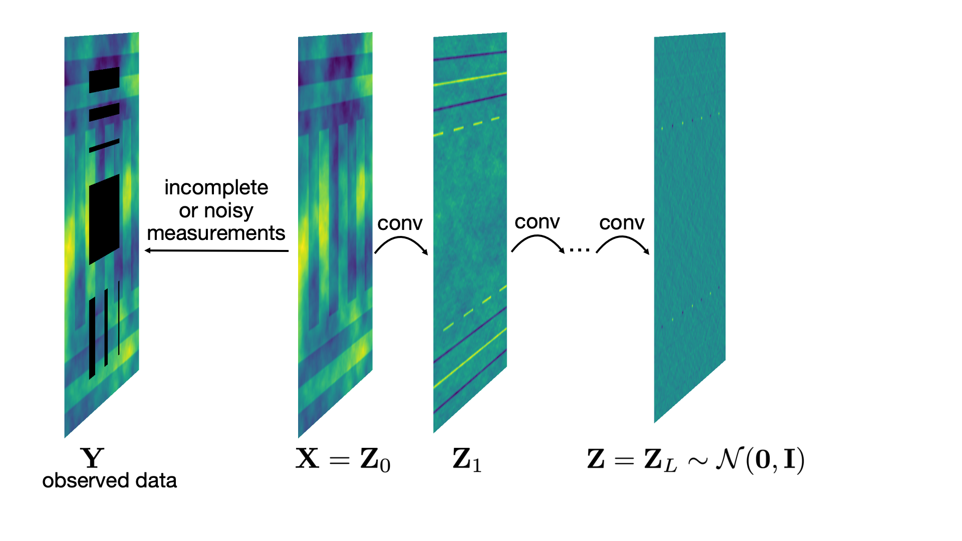
The reason for defining $\mathbf{x}$ through an inverse transform $\mathbf{z}=\mathbf{g}(\mathbf{x})$, rather than a forward transform, is twofold. Firstly, it establishes a formal connection to traditional GMRFs, see Proposition 1 below. Secondly, it gives an AR model with infinite receptive field, meaning that the output prediction at each pixel depends on all the pixels, rather than just on nearby pixels, even for a one-layer model. Compared to dilated CNNs (Yu & Koltun 2015, e.g.), which achieve long (yet finite) range dependencies through several layers of dilated filters, this is a simpler construction.

In this paper, we consider two special forms of convolutional filters: plus ($+$) filters and sequential (seq) filters, with forms

where $a_{1},\ldots,a_{5}\in\mathbb{R}$ are parameters to be learned, and the empty positions are fixed to zero. The benefit of filters with these special designs is that they correspond to transforms for which $\det(\mathbf{G}_{l})$ in Eq. (8) can be cheaply computed.

Defining a linear DGMRF through a sequence of convolutions using different small filters is of course equivalent to defining it using a single convolution with a larger filter, apart from at the boundary. The equivalent larger filter can be obtained by sequentially convolving the smaller filters with themselves. The main motivation for using the deep definition is that it has cheap determinant calculations, using Eq. (8) and the $+$- and seq-filters, which is not the case for a general larger filter. Also, a deep definition results in fewer parameters to learn. For example, four full $3\times 3$-filters has 36 parameters compared to 81 parameters for the corresponding $9\times 9$-filter. Finally, the deep convolutional architecture has proven successful in countless applications of neural networks, which makes it plausible that also GMRFs should benefit from the same inductive biases. The addition of non-linearities between the layers is discussed in Section 3.4. We now discuss the two filter types and their determinant computation for the singlechannel case and discuss the multichannel construction in Section 3.3.

When $C>1$, Eq. (6) can be written on vector form as

where $\mathbf{G}_{l,i,j}$ is the transition matrix of a single convolution from input channel $j$ to output channel $i$, and $b_{l,j}$ is the bias of output channel $j$. In order to make $\det(\mathbf{G}_{l})$ computationally tractable, we set $\mathbf{G}_{l,i,j}=\mathbf{0}$ for $i<j$, making $\mathbf{G}_{l}$ lower block triangular and

The ordering of channels could vary between different layers to allow information to flow back and forth between all channels. One could also add invertible $1\times 1$ convolutions (Kingma & Dhariwal 2018) between layers for this ordering to be dynamic and learnable. A multichannel DGMRF could learn more interesting representations by storing different features in different channels of the hidden layers. Even with singlechannel data, the hidden layers can be multichannel by using a multiscale architecture (Dinh et al. 2017).

The linear DGMRFs can be extended by adding non-linear activation functions between layers of the neural network $\mathbf{g}_{\bm{\theta}}(\mathbf{x})$. Formally, Eq. (6) is replaced by

where $\psi_{l}$ is a non-linear scalar function that operates element-wise. We restrict $\psi_{l}$ to be strictly increasing, to ensure that $\mathbf{g}_{\bm{\theta}}(\mathbf{x})$ is a bijection.

The distribution of $\mathbf{x}$ can now be computed by the change of variable rule

where $\mathbf{h}_{l}=\text{vec}(\text{conv}(\mathbf{Z}_{l-1},\mathbf{w}_{l})+\mathbf{b}_{l})$ is the input to $\psi_{l}$ and $\psi_{l}^{\prime}$ is the derivative. Just as in the linear case, the computational cost of this density is linear.

Per default we assume that $\psi_{l}$ are Parametric Rectified Linear Units (PReLUs), defined by

where $\alpha_{l}$ are learnable parameters with $\alpha_{l}>0$. We can now add $\alpha_{1},\ldots,\alpha_{L}$ to the parameters $\bm{\theta}$ and optimize them jointly.

For the linear DGMRF, the marginal likelihood can be written on closed form as

for arbitrary value of $\mathbf{x}^{*}$. Unfortunately, this expression requires the determinant of the posterior precision matrix $\det(\mathbf{G}^{\top}\mathbf{G}+\sigma^{-2}\mathbf{I}_{\mathbf{m}})$, which is computationally infeasible for large $N$. Instead, we focus on the variational evidence lower bound (ELBO) $\mathcal{L}\left(\bm{\theta},\bm{\phi},\mathbf{y}\right)\leq\log p(\mathbf{y}|\bm{\theta})$ which can be written as

where $q_{\bm{\phi}}(\mathbf{x})$ is the variational posterior approximation, which depends on variational parameters $\bm{\phi}$. We here only intend to use $q_{\bm{\phi}}(\mathbf{x})$ as a means for optimizing $\bm{\theta}$, and not for example to make posterior predictions. For simplicity, we choose $q_{\bm{\phi}}(\mathbf{x})=\mathcal{N}(\mathbf{x}|\bm{\nu},\mathbf{S})$ with diagonal covariance matrix, and $\bm{\phi}=\{\bm{\nu},\mathbf{S}\}$. After inserting the variational and model densities and simplifying, we can write the ELBO as

where constant terms have been omitted, and all parameters have been subscripted with $\bm{\theta}$ and $\bm{\phi}$ to clarify whether they are model or variational parameters. Additionally, we use the reparameterization trick (Kingma & Welling 2013) replacing the last expectation with a sum over $N_{q}$ standard random samples $\bm{\varepsilon}_{1},\ldots,\bm{\varepsilon}_{N_{q}}$, and set $\mathbf{x}_{i}=\bm{\nu}_{\bm{\phi}}+\mathbf{S}_{\bm{\phi}}^{1/2}\bm{\varepsilon}_{i}$ in the sum. This gives an unbiased estimator of the ELBO, which has low variance. Moreover, this estimator is differentiable with respect to $\bm{\theta}$ and $\bm{\phi}$ and can be used for stochastic gradient optimization with autodiff and backprop. Parameter learning will be fast, with a time complexity that is $\mathcal{O}(N)$ for a fixed number of iterations of optimization, since backprop in a CNN is linear and so are the determinant computations described in Section 3.2. This can be compared with $\mathcal{O}(N^{3})$ for standard GP and $\mathcal{O}(N^{3/2})$ for standard GMRF inference in 2D problems, based on the Cholesky-decomposition. The ELBO can be trivially extended to the non-linear model by replacing $\log|\det(\mathbf{G}_{\bm{\theta}})|$ in Eq. (10).

For a linear DGMRF, the conditional posterior $p(\mathbf{x}|\hat{\bm{\theta}},\mathbf{y})$ is also a GMRF, see Eq. (5). Even though computing this density is too costly in general, it is possible to compute the posterior mean and to draw samples from the posterior, which can be used for making predictions. Both require solving linear equation systems $\tilde{\mathbf{Q}}\mathbf{x}=\mathbf{c}$ involving the posterior precision matrix $\tilde{\mathbf{Q}}=\mathbf{G}^{\top}\mathbf{G}+\sigma^{-2}\mathbf{I}_{\mathbf{m}}$. For this we use the conjugate gradient (CG) method (see e.g. Barrett et al. 1994), which is an iterative method that, rather than exactly computing $\mathbf{x}=\tilde{\mathbf{Q}}^{-1}\mathbf{c}$, iteratively minimizes the relative residual $\|\tilde{\mathbf{Q}}\mathbf{x}-\mathbf{c}\|/\|\mathbf{c}\|$ until it falls below some threshold $\delta$, that can be set arbitrarily low. In practice, $\delta=10^{-7}$ gives solutions that visually appear to be identical to the exact solution. CG only requires matrix-vector-multiplications, which means that the multiplications with $\mathbf{G}$ and $\mathbf{G}^{\top}$ can be implemented in a matrix-free fashion using convolution.

Posterior sampling for $\mathbf{x}$ can be performed using the method of Papandreou & Yuille 2010 by computing

where $\mathbf{u}_{1}$ and $\mathbf{u}_{2}$ are standard Gaussian random vectors. It can be easily verified that $\mathbf{x}_{s}$ is Gaussian, with the same mean and covariance as the posterior.

Given a number of posterior samples, the posterior marginal variances $\text{Var}(x_{i}|\mathbf{y},\hat{\bm{\theta}})$ can be naively approximated using Monte Carlo estimation, but more efficiently approximated using the simple Rao-Blackwellized Monte Carlo (simple RBMC) method by Sidén et al. 2018. This provides a way to compute the posterior predictive uncertainty as

The time complexity is here mainly decided by the complexity of the CG method, which can be described as $\mathcal{O}(N\sqrt{\kappa})$, where $\kappa$ is the condition number of $\tilde{\mathbf{Q}}$ (Shewchuk 1994). It is difficult to say how $\kappa$ depends on $N$ for a general $\tilde{\mathbf{Q}}$, but for a two-dimensional, second-order elliptic boundary value problems, for example the SPDE approach with $\gamma=1$, $\kappa$ is linear in $N$ so the method is $\mathcal{O}(N^{3/2})$. Even though this is the same as for the sparse Cholesky method, we have observed CG to be a lot faster in practice. Also, the storage requirements for CG is $\mathcal{O}(N)$, versus $\mathcal{O}(N\log N)$ for Cholesky.

A drawback with non-linear DGMRFs is that they do not give a simple posterior $p(\mathbf{x}|\hat{\bm{\theta}},\mathbf{y})$. We could use the variational approximation $q_{\bm{\phi}}(\mathbf{x})$ instead, but the proposed Gaussian independent variational family is probably too simple to approximate the true posterior in a satisfying way. We discuss possible solutions to this limitation in Section 7.

The inference algorithm is summarized in Algorithm 1.

GMRFs have a long history in spatial and image analysis (see e.g. Woods 1972; Besag 1974 and Rue & Held 2005). The mentioned SPDE approach has been extended in numerous ways leading to flexible GMRF models, with for example non-stationarity (Fuglstad et al. 2015), oscillation (Lindgren et al. 2011) and non-Gaussianity (Bolin 2014). A nested (deep) SPDE is introduced by Bolin & Lindgren 2011, which results in a model similar to ours, but which lacks the connection to CNNs and some of the computational advantages that we provide.

Papandreou & Yuille 2010 use GMRFs for inpainting in natural images, in combination with CG to obtain posterior samples. They do not learn the form of the prior precision matrix, but instead rewrite the model as a product of Gaussian experts, and learn the mean and variance of the Gaussian factors. Papandreou & Yuille 2011 assume a heavy-tailed non-Gaussian prior for the latent pixel values, and use a variational GMRF approximation for the posterior.

GPs (Stein 1999; Williams & Rasmussen 2006) are commonplace for modelling spatially dependent data, not necessarily restricted to observations on the grid. The GP covariance kernel, which encodes the spatial dependencies, can be made flexible (Wilson & Adams 2013) and deep (Dunlop et al. 2018; Roininen et al. 2019). However, standard GPs are limited by $\mathcal{O}(N^{3})$ computational complexity (assuming the number of measurements $M\sim\mathcal{O}(N)$).

Inducing point methods (Quiñonero-Candela & Rasmussen 2005; Snelson & Ghahramani 2006) can reduce the complexity to $\mathcal{O}(P^{2}N+P^{3})$ or even $\mathcal{O}(P^{3})$ (Hensman et al. 2013), where $P$ is the number of inducing points. However, for grid data, these methods tend to over-smooth the data (Wilson & Nickisch 2015) unless $P$ is chosen in the same order of magnitude as $N$. When the data are on a regular grid and fully observed, Kronecker and Toeplitz methods can be used for fast computation (e.g. Saatçi 2011; Wilson 2014). Under certain assumptions about the interactions across the input dimensions, such as additivity and separability, this can reduce the complexity to $\mathcal{O}(N\log N)$. These methods can also be extended to when the data are not on the grid (Wilson & Nickisch 2015), or when the grid is incomplete (Stroud et al. 2016).

Deep generative models are normally trained on large datasets, and can then be used to generate new samples from the data distribution, or to explore learned latent representations. For example, generative adversarial networks (GANs, Goodfellow et al. 2014) have been used for inpainting problems in natural images (see e.g. Yu et al. 2018; Liu et al. 2018) with impressive results. Our model is mainly targeted at smaller datasets, as single images, where too complex models are likely to overfit. Instead, we achieve an infinite receptive field through the inverse definition $\mathbf{z}=\mathbf{g}(\mathbf{x})$, which require few parameters. Also, linear DGMRFs can readily provide uncertainty estimates, which is prohibitive for most deep generative models. Overall, deep generative models are difficult to use for typical spatial problems, but these models share ideas with our proposed model as we discuss below.

Flow-based or invertible generative models, e.g., NICE (Dinh et al. 2014), normalizing flows (Rezende & Mohamed 2015), IAF (Kingma et al. 2016), MAF (Papamakarios et al. 2017), real NVP (Dinh et al. 2017), Glow (Kingma & Dhariwal 2018) and i-ResNet (Behrmann et al. 2019), model $\mathbf{x}$ as a bijective function of a latent variable from a simple base distribution, just as our model. The likelihood can be optimized directly for parameter learning, but generally require all pixels to be non-missing, that is, these methods are not designed to handle the situation with incomplete or noisy observations that we are considering. One connection to our work is that a linear DGMRF with seq-filters can be seen as a fully linear MAF with masked convolutional MADE-layers. Dinh et al. 2014 use a learned model for inpainting with projected gradient ascent, which gives the posterior mode but no uncertainty quantification. Lu & Huang 2019 provide a conditional version of Glow for inpainting, but this requires missing pixels to be known during training, and the predictive distribution is modeled directly and not through a Bayesian inversion of the model.

Auto-regressive models, e.g. PixelRNN (Van den Oord et al. 2016a), PixelCNN (Van den Oord et al. 2016b) and PixelCNN++ (Salimans et al. 2017), model the pixel values sequentially similarly to our proposed seq-filters, but there are some major differences. The seq-filters use masked convolutions to obtain cheap determinant computations and the ordering of pixels can change between layers, whereas auto-regressive models have no latent variables and are trained using the same image as input and output. (Van den Oord et al. 2016a) consider image completion, but are limited to the e.g. the case where the bottom half of the image is missing, and can’t handle a general mask.

Variational autoencoders (Kingma & Welling 2013) differ from our model in that they use the deep transform of the latent variables for modeling the parameters of the distribution of the data, rather than for the data directly. This makes the recovery of the latent variables intractable, which is not the case for our model, however, we still use the same variational optimization algorithm for speedups.

Deep image prior (DIP, Ulyanov et al. 2018) uses CNNs, trained on single images, for denoising and inpainting, with promising results. However, this is not truly a probabilistic generative model, since the latent variables are not inferred, but fixed to some initial random values. Thus, it would be difficult to output predictive uncertainty from such a model.

We demonstrate the behaviour of our model for an inpainting problem on the two toy datasets in Figure 2, which have size 160$\times$120 pixels. The data in the first row are generated as a random sample from the Matérn GMRF in Eq. (4) with $\gamma=1$, $\tau=1$, and $\kappa^{2}=8/50^{2}$ corresponding to a spatial correlation range of 50 pixels. The data in the second row are the same, but we have added horizontal and vertical edges, to investigate the model’s ability to capture such patterns. Column 2 shows the posterior mean for $\mathbf{x}$ when the Matérn model with the same hyperparameters is used for prediction, which gives optimal results for the first row, but which over-smooths the edges in the second row. The corresponding results for different instances of the linear DGMRF, are shown in column 3-6. They all perform well in the simple case without edges, in which the $+$-filter models contain the true model according to Proposition 1. In the case with edges, the model with depth $L=1$ which corresponds to a standard GMRF is too simple to handle the more complex structure in the data, but for $L=3$, all the models give reasonable results, that preserve the edges.

Figure 3 displays the learned $+$-filters of the 3-layer model, and the values of valid pixels of the hidden layers, when original data, including missing pixels, are used as input. The first two filters learns differentiation in the vertical and horizontal direction, and the third filter is close to an identity function. Most spatial structure is removed in layer 3, that is assumed to be standard normal by the model.

We compare our method against some popular methods for large data sets in spatial statistics, by considering the satellite data of daytime land surface temperatures, used in the competition by Heaton et al. 2018. The data are on a 500$\times$300 grid, with 105,569 non-missing observations as training set. The test set consists of 42,740 observations and have been selected as the pixels that were missing due to cloud cover on a different date. The dataset and the missing pixels are shown in the supplement, together with the posterior output from our model. The data and code for some of the methods can be found at https://github.com/finnlindgren/heatoncomparison. The participants of the competition were instructed to use exponential correlation if applicable, and to add a constant mean and linear effects of the latitude and longitude. For this reason, we extend the measurement equation to include linear trends, so that

where $\mathbf{F}$ is a spatial covariate matrix with columns corresponding to (constant, longitude, latitude), and $\bm{\beta}$ is a 3-dimensional regression coefficient vector, which can be integrated out jointly with $\mathbf{x}$ for the predictions, see details in the supplement.

Table 1 compares different instances of our model with the methods in the competition, which are briefly described in the supplement, and in more detail in Heaton et al. 2018. One of the top competitors, SPDE, is essentially the same method as described in Section 2.3. For comparison with another deep method, we have also included results for DIP using the authors own implementation²² 2 https://github.com/DmitryUlyanov/deep-image-prior. For DIP, removal of linear trends and normalization to $[0,1]$ were done in preprocessing, and these steps were inverted before evaluation. As DIP does not give uncertainty estimates, we also compare with an ensemble of 10 DIP models, using the ensemble mean and standard deviation as predictive distribution. The scores used are mean absolute error (MAE), root-mean-squared-error (RMSE), mean continuous rank probability score (CRPS), mean interval score (INT), and prediction interval coverage (CVG). CRPS and INT are proper scoring rules, that also account for the predictive uncertainty (Gneiting & Raftery 2007). These are the same scores that were used in the competition.

For the DGMRFs, based on the first three scores, the seq-filters of size 5$\times$5 perform better compared to those of size 3$\times$3 and the $+$-filters, which may be due to the increased flexibility of larger filters. Moreover, deeper models tend to give better results. For the non-linear (NL) model, CG cannot be used to compute posterior mean and uncertainty, and the first two scores are instead computed based on the mean of the variational approximation. We note that the NL model performs worse than the linear. Our primary explanation for this disappointing result is that the variational posterior is insufficient in approximating the true posterior. An independent distribution naturally has limited ability to approximate a spatially dependent posterior, and empirically we have also seen that the variational approximation for the linear model performs much worse than the true posterior (results not shown). DGMRF outperforms all the methods from the competition on all criteria except CVG, where it is slightly worse than NNGP. In terms of MAE, RMSE and CRPS the improvement is substantial. It is difficult to compare computing times due to different hardware, but our method takes roughly 2.5h for the $\text{seq}_{5\times 5,L=5}$ model using a Tesla K40 GPU, out of which roughly 95% of the time is for parameter learning.

References

- Abadi et al. (2016) Abadi, M., Barham, P., Chen, J., Chen, Z., Davis, A., Dean, J., Devin, M., Ghemawat, S., Irving, G., Isard, M., et al. Tensorflow: A system for large-scale machine learning. In 12th USENIX Symposium on Operating Systems Design and Implementation (OSDI 16), pp. 265–283, 2016.
- Barrett et al. (1994) Barrett, R., Berry, M. W., Chan, T. F., Demmel, J., Donato, J., Dongarra, J., Eijkhout, V., Pozo, R., Romine, C., and Van der Vorst, H. Templates for the solution of linear systems: building blocks for iterative methods, volume 43. Siam, Philadelphia, PA, 1994.
- Behrmann et al. (2019) Behrmann, J., Grathwohl, W., Chen, R. T. Q., Duvenaud, D., and Jacobsen, J.-H. Invertible residual networks. In Chaudhuri, K. and Salakhutdinov, R. (eds.), Proceedings of the 36th International Conference on Machine Learning, volume 97 of Proceedings of Machine Learning Research, pp. 573–582, Long Beach, California, USA, 09–15 Jun 2019. PMLR. URL http://proceedings.mlr.press/v97/behrmann19a.html.
- Besag (1974) Besag, J. Spatial interaction and the statistical analysis of lattice systems. Journal of the Royal Statistical Society. Series B (Methodological), 36(2):192–236, 1974.
- Bolin (2014) Bolin, D. Spatial matérn fields driven by non-gaussian noise. Scandinavian Journal of Statistics, 41(3):557–579, 2014.
- Bolin & Lindgren (2011) Bolin, D. and Lindgren, F. Spatial models generated by nested stochastic partial differential equations, with an application to global ozone mapping. Annals of Applied Statistics, 5(1):523–550, 2011.
- Dinh et al. (2014) Dinh, L., Krueger, D., and Bengio, Y. Nice: Non-linear independent components estimation. arXiv preprint arXiv:1410.8516, 2014.
- Dinh et al. (2017) Dinh, L., Sohl-Dickstein, J., and Bengio, S. Density estimation using real NVP. arXiv preprint arXiv:1605.08803, 2017.
- Dunlop et al. (2018) Dunlop, M. M., Girolami, M. A., and Stuart, A. M. How Deep Are Deep Gaussian Processes? Journal of Machine Learning Research, 19:1–46, 2018.
- Fuglstad et al. (2015) Fuglstad, G.-A., Lindgren, F., Simpson, D., and Rue, H. Exploring a new class of non-stationary spatial Gaussian random fields with varying local anisotropy. Statistica Sinica, 25(1):115–133, 2015.
- Gneiting & Raftery (2007) Gneiting, T. and Raftery, A. E. Strictly proper scoring rules, prediction, and estimation. Journal of the American statistical Association, 102(477):359–378, 2007.
- Goodfellow et al. (2014) Goodfellow, I., Pouget-Abadie, J., Mirza, M., Xu, B., Warde-Farley, D., Ozair, S., Courville, A., and Bengio, Y. Generative adversarial nets. In Advances in neural information processing systems, pp. 2672–2680, 2014.
- Guinness & Fuentes (2017) Guinness, J. and Fuentes, M. Circulant embedding of approximate covariances for inference from gaussian data on large lattices. Journal of computational and Graphical Statistics, 26(1):88–97, 2017.
- Heaton et al. (2018) Heaton, M. J., Datta, A., Finley, A. O., Furrer, R., Guinness, J., Guhaniyogi, R., Gerber, F., Gramacy, R. B., Hammerling, D., Katzfuss, M., Lindgren, F., Nychka, D. W., Sun, F., and Zammit-mangion, A. A Case Study Competition Among Methods for Analyzing Large Spatial Data. Journal of Agricultural, Biological and Environmental Statistics, 24(3):398–425, 2018. doi: 10.1007/s13253-018-00348-w.
- Hensman et al. (2013) Hensman, J., Fusi, N., and Lawrence, N. D. Gaussian Processes for Big Data. In Uncertainty in Artificial Intelligence (UAI), 2013.
- Kingma & Dhariwal (2018) Kingma, D. P. and Dhariwal, P. Glow : Generative Flow with Invertible 1x1 Convolutions. In Advances in Neural Information Processing Systems, pp. 10215–10224, 2018.
- Kingma & Welling (2013) Kingma, D. P. and Welling, M. Auto-Encoding Variational Bayes. arXiv preprint arXiv:1312.6114, 2013.
- Kingma et al. (2016) Kingma, D. P., Salimans, T., Jozefowicz, R., Chen, X., Sutskever, I., and Welling, M. Improved variational inference with inverse autoregressive flow. In Advances in neural information processing systems, pp. 4743–4751, 2016.
- Lindgren et al. (2011) Lindgren, F., Rue, H., and Lindström, J. An explicit link between Gaussian fields and Gaussian Markov random fields: The SPDE approach. Journal of the Royal Statistical Society Series B, 73(4):423–498, 2011.
- Liu et al. (2018) Liu, G., Reda, F. A., Shih, K. J., Wang, T.-C., Tao, A., and Catanzaro, B. Image inpainting for irregular holes using partial convolutions. In Proceedings of the European Conference on Computer Vision (ECCV), pp. 85–100, 2018.
- Ljung (1999) Ljung, L. System identification, Theory for the user. System sciences series. Prentice Hall, Upper Saddle River, NJ, USA, second edition, 1999.
- Lu & Huang (2019) Lu, Y. and Huang, B. Structured Output Learning with Conditional Generative Flows. arXiv preprint arXiv:1905.13288, 2019.
- Papamakarios et al. (2017) Papamakarios, G., Pavlakou, T., and Murray, I. Masked autoregressive flow for density estimation. In Advances in Neural Information Processing Systems, pp. 2338–2347, 2017.
- Papandreou & Yuille (2010) Papandreou, G. and Yuille, A. Gaussian sampling by local perturbations. Advances in Neural Information Processing Systems 23, 90(8):1858–1866, 2010.
- Papandreou & Yuille (2011) Papandreou, G. and Yuille, A. L. Efficient variational inference in large-scale Bayesian compressed sensing. 2011 IEEE International Conference on Computer Vision Workshops (ICCV Workshops), pp. 1332–1339, 2011.
- Quiñonero-Candela & Rasmussen (2005) Quiñonero-Candela, J. and Rasmussen, C. E. A unifying view of sparse approximate gaussian process regression. Journal of Machine Learning Research, 6(Dec):1939–1959, 2005.
- Rezende & Mohamed (2015) Rezende, D. and Mohamed, S. Variational inference with normalizing flows. In Proceedings of the 32nd International Conference on Machine Learning, pp. 1530–1538, 2015.
- Roininen et al. (2019) Roininen, L., Girolami, M., Lasanen, S., and Markkanen, M. Hyperpriors for Matérn fields with applications in Bayesian inversion. Inverse Problems & Imaging, 13:1–29, 2019. URL http://aimsciences.org//article/id/d17bde6b-3e5f-438d-af0a-b712cf433748.
- Rue & Held (2005) Rue, H. and Held, L. Gaussian Markov random fields: theory and applications. CRC Press, 2005.
- Saatçi (2011) Saatçi, Y. Scalable Inference for Structured Gaussian Process Models. PhD thesis, University of Cambridge, 2011.
- Salimans et al. (2017) Salimans, T., Karpathy, A., Chen, X., and Kingma, D. P. Pixelcnn++: Improving the pixelcnn with discretized logistic mixture likelihood and other modifications. arXiv preprint arXiv:1701.05517, 2017.
- Shewchuk (1994) Shewchuk, J. R. An introduction to the conjugate gradient method without the agonizing pain. Technical Report CS-94-125, Carnegie Mellon University, 1994.
- Sidén et al. (2018) Sidén, P., Lindgren, F., Bolin, D., and Villani, M. Efficient covariance approximations for large sparse precision matrices. Journal of Computational and Graphical Statistics, 27(4):898–909, 2018.
- Snelson & Ghahramani (2006) Snelson, E. and Ghahramani, Z. Sparse gaussian processes using pseudo-inputs. In Advances in neural information processing systems, pp. 1257–1264, 2006.
- Stein (1999) Stein, M. L. Interpolation of spatial data: some theory for kriging. Springer, 1999.
- Stroud et al. (2016) Stroud, J. R., Stein, M. L., and Lysen, S. Bayesian and Maximum Likelihood Estimation for Gaussian Processes on an Incomplete Lattice. Journal of Computational and Graphical Statistics, 26(1):108–120, 2016.
- Ulyanov et al. (2018) Ulyanov, D., Vedaldi, A., and Lempitsky, V. Deep image prior. In Proceedings of the IEEE Conference on Computer Vision and Pattern Recognition, pp. 9446–9454, 2018.
- Van den Oord et al. (2016a) Van den Oord, A., Kalchbrenner, N., and Kavukcuoglu, K. Pixel Recurrent Neural Networks. arXiv preprint arXiv:1601.06759, 2016a.
- Van den Oord et al. (2016b) Van den Oord, A., Kalchbrenner, N., Vinyals, O., Espeholt, L., Graves, A., and Kavukcuoglu, K. Conditional Image Generation with PixelCNN Decoders. In Advances in neural information processing systems, 2016b.
- Whittle (1954) Whittle, P. On stationary processes in the plane. Biometrika, 41:434–449, 1954.
- Whittle (1963) Whittle, P. Stochastic processes in several dimensions. Bulletin of the International Statistical Institute, 40(2):974–994, 1963.
- Williams & Rasmussen (2006) Williams, C. K. and Rasmussen, C. E. Gaussian processes for machine learning. MIT press Cambridge, MA, 2006.
- Wilson & Adams (2013) Wilson, A. and Adams, R. Gaussian process kernels for pattern discovery and extrapolation. In International Conference on Machine Learning, pp. 1067–1075, 2013.
- Wilson & Nickisch (2015) Wilson, A. and Nickisch, H. Kernel interpolation for scalable structured gaussian processes (kiss-gp). In International Conference on Machine Learning, pp. 1775–1784, 2015.
- Wilson (2014) Wilson, A. G. Covariance kernels for fast automatic pattern discovery and extrapolation with Gaussian processes. PhD thesis, University of Cambridge, 2014.
- Woods (1972) Woods, J. W. Two-Dimensional Discrete Markovian Fields. IEEE Transactions on Information Theory, 18(2):232–240, 1972.
- Xu et al. (2019) Xu, K., Hu, W., Leskovec, J., and Jegelka, S. How powerful are graph neural networks? In International Conference on Learning Representations, 2019. URL https://openreview.net/forum?id=ryGs6iA5Km.
- Yu & Koltun (2015) Yu, F. and Koltun, V. Multi-scale context aggregation by dilated convolutions. arXiv preprint arXiv:1511.07122, 2015.
- Yu et al. (2018) Yu, J., Lin, Z., Yang, J., Shen, X., Lu, X., and Huang, T. S. Generative image inpainting with contextual attention. In Proceedings of the IEEE conference on computer vision and pattern recognition, pp. 5505–5514, 2018.
Supplementary material
Proof of Proposition 2
The transform matrix can be written as
where denotes the Kronecker sum and the Kronecker product, is a tridiagonal Toeplitz matrix, denoted , meaning that
and similarly . For the eigenvalues of a Kronecker sum, it holds that if is an eigenvalue of and is an eigenvalue of , then is an eigenvalue of (Graham 1981). Moreover, the eigenvalues of a tridiagonal Toeplitz matrix have a simple formula
which holds for real and complex , and (Smith 1985). Substituting this formula into the expression
gives the result in Proposition 2.
-Filter Reparameterization
The following reparameterization is used to ensure that has real positive eigenvalues
where are real numbers.
Implementation Details
The model parameters and variational parameters are trained with respect to the negative ELBO (Eq. (10)) divided by as loss function, using Adam optimization (Kingma & Ba 2014) with default settings, learning rate and k iterations. The parameters with the lowest loss value are then saved and conditioned on by our implementation of the CG algorithm, for computing the posterior mean and standard deviation of . We use samples from variational approximation to compute the expectation in each iteration. We can train the measurement error together with the other parameters , but we have used a fixed , which seems to give very similar results, but with somewhat faster convergence. For the DGMRFs with seq-filters, we randomly select among the eight possible orientations of the filters in each layer. As the toy data is centered around 0, the bias in each layer was fixed to 0 for this experiment. The satellite data was normalized to have maximum pixel value 1.
Competing Methods
We here briefly describe the methods that are compared against in Table 1, except DIP that is mentioned in Section 5.3. For more details we refer to Heaton et al. 2018.
FRK (Fixed rank kriging) (Zammit-Mangion & Cressie 2017) approximates a spatial process using a linear combination of spatial basis functions with .
Gapfill (Gerber et al. 2018) is an algorithmic, distribution free method that makes predictions using sorting and quantile regression based on closeby pixels.
LatticeKrig (Nychka et al. 2015) approximates a GP with a linear combination of multi-resolution basis function with weights that follow a certain GMRF.
LAGP (Local approximate Gaussian process) (Gramacy & Apley 2015) fits a GP, but only uses the subset of points in the training data that are closest to the points in the test data.
MetaKriging (Guhaniyogi et al. 2017) is an approximate Bayesian method that splits the training data into subsets, fits one model to each subset, and combines them all into a meta-posterior, here using GPs.
MRA (Multi-resolution approximation) (Katzfuss 2017) uses a multi-resolution approximation of a GP, similar to LatticeKrig, but uses compactly supported basis functions.
NNGP (Nearest-neighbor Gaussian process) (Datta et al. 2016) approximates a GP by rewriting the joint density of the data points as a product of conditional densities, and truncating the conditioning sets to only contain the nearest neighbors.
Partition makes a spatial partitioning (splits the domain into disjoint subsets) and fits spatial basis functions to each partition, similar to FRK, but with some parameters shared between partitions.
Pred. Proc. (Predictive processes) (Finley et al. 2009) approximates a GP using a set of knot locations, also known as inducing points, with which reduces the size of the covariance matrix that needs to be inverted.
SPDE (Stochastic partial differential equation) (Lindgren et al. 2011) represents a GP with a GMRF (see Section 2.3).
Tapering (Furrer et al. 2006) obtains an approximation of a GP with sparse covariance matrix by truncating small covariances in a way that preserves positive definiteness.
Peri. Embe. (Periodic embedding) (Guinness & Fuentes 2017) approximates a GP using the fast Fourier transform on a regular grid.
Linear Trend Model
For inference with the linear trend model in Eq. (11), we extend the vector of latents to include also the regression coefficients , and use (for linear DGMRFs) the prior
where can be interpreted as the prior inverse standard deviation of the elements of , which we fix at . The posterior for is a GMRF, similar to Eq. (5), with
and thus we can proceed with inference as before, with instead of , with slight modifications to the ELBO and to the CG method. We use an independent variational approximation for . Integrating out is important for the predictive performance. For reference, if linear trends are instead removed using the ordinary least squares estimates of in a preprocessing step, the row in Table 1 corresponding to instead reads (1.25, 1.74, 0.90, 8.45, 0.89). When the linear trend model is used, we compute posterior standard deviations using standard Monte Carlo estimates, instead of simple RBMC, using samples.