Multi-Objective Actor-Critics for Real-Time Bidding in Display AdvertisingThanks: This work was supported by the National Key R&D Program of China [2020YFB1707903]; the National Natural Science Foundation of China [61872238, 61972254]; Shanghai Municipal Science and Technology Major Project [2021SHZDZX0102]; the CCF-Tencent Open Fund [RAGR20200105] and the Tencent Marketing Solution Rhino-Bird Focused Research Program [FR202001]. Chaoqi Yang completed this work when he was an undergraduate student at Shanghai Jiao Tong University. Xiaofeng Gao is the corresponding author.
Abstract
Online Real-Time Bidding (RTB) is a complex auction game among which advertisers struggle to bid for ad impressions when a user request occurs. Considering display cost, Return on Investment (ROI), and other influential Key Performance Indicators (KPIs), large ad platforms try to balance the trade-off among various goals in dynamics. To address the challenge, we propose a Multi-ObjecTive Actor-Critics algorithm based on reinforcement learning (RL), named MoTiAC, for the problem of bidding optimization with various goals. In MoTiAC, objective-specific agents update the global network asynchronously with different goals and perspectives, leading to a robust bidding policy. Unlike previous RL models, the proposed MoTiAC can simultaneously fulfill multi-objective tasks in complicated bidding environments. In addition, we mathematically prove that our model will converge to Pareto optimality. Finally, experiments on a large-scale real-world commercial dataset from Tencent verify the effectiveness of MoTiAC versus a set of recent approaches.
Keywords:
Real-time Bidding Reinforcement Learning Display Advertising Multiple Objectives1 Introduction
The rapid development of the Internet and smart devices has created a decent environment for the advertisement industry. As a result, real-time bidding (RTB) has gained continuous attention in the past few decades [23]. A typical RTB setup consists of publishers, supply-side platforms (SSP), data management platforms (DMP), ad exchange (ADX), and demand-side platforms (DSP). When an online browsing activity triggers an ad request in one bidding round, the SSP sends this request to the DSP through the ADX, where eligible ads compete for the impression. The bidding agent, DSP, represents advertisers to come up with an optimal bid and transmits the bid back to the ADX (e.g., usually within less than 100ms [23]), where the winner is selected to be displayed and charged by a generalized second price (GSP).
In the RTB system, bidding optimization in DSP is regarded as the most critical problem [24]. Unlike Sponsored Search (SS) [25], where advertisers make keyword-level bidding decisions, DSP in the RTB setting needs to calculate the optimal impression-level bidding under the basis of user/customer data (e.g., income, occupation, purchase behavior, gender, etc.), target ad (e.g., content, click history, budget plan, etc.) and auction context (e.g., bidding history, time, etc.) in every single auction [24].
Thus, our work focuses on DSP, where bidding optimization happens. In real-time bidding, two fundamental challenges need to be addressed. Firstly, the RTB environment is highly dynamic. In [20, 24, 26], researchers make a strong assumption that the bidding process is stationary over time. However, the sequence of user queries (e.g., incurring impressions, clicks, or conversions) is time-dependent and mostly unpredictable [25], where the outcome influences the next auction round. Traditional algorithms usually learn an independent predictor and conduct fixed optimization that amounts to a greedy strategy, often not leading to the optimal return [3]. Agents with reinforcement learning (RL) address the aforementioned challenge to some extent [7, 12, 25]. RL-based methods can alleviate the instability by learning from immediate feedback and long-term reward. However, these methods are limited to either Revenue or ROI, which is only one part of the overall utility. In the problem of RTB, we assume that the utility is two-fold, as outlined: (i) the cumulative cost should be kept within the budget; (ii) the overall revenue should be maximized. Therefore, the second challenge is that the real-world RTB industry needs to consider multiple objectives, which are not adequately addressed in the existing literature.
To address the challenges mentioned above, we propose a Multi-Objective Actor-Critic model, named MoTiAC. We generalize the popular asynchronous advantage actor-critic (A3C) [13] reinforcement learning algorithm for multiple objectives in the RTB setting. Our model employs several local actor-critic networks with different objectives to interact with the same environment and then updates the global network asynchronously according to different reward signals. Instead of using a fixed linear combination of different objectives, MoTiAC can decide on adaptive weights over time according to how well the current situation conforms with the agent’s prior. We evaluate our model on click data collected from the Tencent ad bidding system. The experimental results verify the effectiveness of our approach versus a set of baselines.
The contributions in this paper can be summarized as follows:
- •
We identify two critical challenges in RTB and are well motivated to use multi-objective RL as the solution.
- •
We propose a novel multi-objective actor-critic model MoTiAC for optimal bidding and prove the superiority of our model from the perspective of Pareto optimality.
- •
Extensive experiments on a real industrial dataset collected from the Tencent ad system show that MoTiAC achieves state-of-the-art performance.
2 Preliminaries
2.1 Definition of oCPA and Bidding Process
In the online advertising scenario, there are three main ways of pricing. Cost-per-mille (CPM) [7] is the first standard, where revenue is proportional to impression. Cost-per-click (CPC) [24] is a performance-based model, i.e., only when users click the ad can the platform get paid. In the cost-per-acquisition (CPA) model, the payment is attached to each conversion event. Regardless of the pricing ways, ad platforms always try to maximize revenue while simultaneously maintaining the overall cost within the budget predefined by advertisers.
In this work, we focus on one pricing model that is currently used in Tencent online ad bidding systems, called optimized cost-per-acquisition (oCPA), in which advertisers are supposed to set a target CPA price, denoted by for each conversion while the charge is based on each click. The critical point for the bidding system is to make an optimal strategy to allocate overall impressions among ads properly, such that (i) the real click-based cost is close to the estimated cost calculated from , specifically,
| (1) |
where is the cost charged by the second highest price and is pre-defined for each conversion; (ii) more overall conversions. In the system, the goal of our bidding agent is to generate an optimal price, adjusting the winner of each impression. We denote as bidding iterations, as a set of all advertisements. For each iteration , , our bidding agent will decide on a to play auction. Then the ad with the highest wins the impression and then receives possible (charged by per click) and based on user engagements.
2.2 Optimization Goals in Real-Time Bidding
On the one hand, when is set higher, ads are more likely to win this impression to get clicks or later conversions, and vice versa. However, on the other hand, higher means lower opportunities for other ad impressions. Therefore, to determine the appropriate bidding price, we define the two optimization objectives as follows:
Objective 1: Minimize overall CPA.
The first objective in RTB bidding problem is to allocate impression-level bids in every auction round, so that each ad will get reasonble opportunities for display and later get clicks or conversions, which makes close to pre-defined by the advertisers:
| (2) |
To achieve the goal of minimizing overall CPA, i.e., be in line with the original budget, a lower ratio between and is desired. Precisely, when the ratio is smaller than 1, the agent will receive a positive feedback. On the contrary, when the ratio is greater than 1, it means that the actual expenditure exceeds the budget and the agent will be punished by a negative reward.
Objective 2: Maximize conversions.
The second objective is to enlarge conversions as much as possible under the condition of a reasonable , so that platform can stay competitive and run a sustainable business:
| (3) |
where is a cumulative value until the current bidding auction. Obviously, relatively high #conversions will receive a positive reward. When the policy network gives fewer conversions, the agent will be punished with a negative reward.
Note that in the real setting, optimization objectives used by advertising platforms can be adjusted based on actual business needs. In the implementation and evaluation of MoTiAC, we use ROI (Return on Investment) and Revenue, corresponding to the two objectives for optimization, i.e., minimizing overall CPA and maximizing the number of conversions. Their definition will be detailed in Sec. 4.1.
3 Methodology
As shown in Sec. 2.1, the RTB problem is a multi-objective optimization problem. We need to control advertisers’ budgets and make profitable decisions for the ad platform. Traditional RTB control policy or RL agent can hardly handle these challenges. In this work, we design MoTiAC to decouple the training procedure of multiple objectives into disentangled worker groups of actor-critics. We will elaborate on the technical details of MoTiAC in the following subsections.
3.1 Asynchronous Advantage Actor-Critic Model in RTB
An actor-critic reinforcement learning setting [8] in our RTB scenario consists of:
- •
state : each state is composed of anonymous feature embeddings extracted from the user profile and bidding environment, indicating the current bidding state.
- •
action : action is defined as the bidding price for each ad based on the input state. Instead of using discrete action space [20], our model outputs a distribution so that action can be sampled based on probability.
- •
reward : obviously, the reward is a feedback signal from the environment to evaluate how good the previous action is, which guides the RL agent towards a better policy. In our model, we design multiple rewards based on different optimization goals. Each actor-critic worker group deals with one type of reward from the environment and later achieves multiple objectives together.
- •
policy : policy is represented as , which denotes the probability to take action under state . In an actor-critic thread, actor works as a policy network, and critic stands for value function of each state. The parameters are updated according to the experience reward obtained during the training process.

For each policy , we define the utility function as
| (4) |
where denotes the distribution of trajectories under policy , and is a return function over trajectory , calculated by summing all the reward signals in the trajectory. The utility function is used to evaluate the quality of an action taken in a specific state. We also introduce value function from critic to reduce the varaition that may occur when updating parameters in real time. After collecting a number of tuples from each trajectory , the policy network is updated by
| (5) |
where represents the learning rate of policy network, is a preset maximum step size in a trajectory, denotes the cumulative discounted reward, and is a decaying factor. The critic network, , could also be updated by:
| (6) |
where represents the learning rate of value function.
3.2 Adaptive Reward Partition
In this subsection, we consider the general -objective case, where is the total number of objectives. As stated in Sec. 2.2, multiple objectives should be considered in modeling the RTB problem. One intuitive way [14] of handling multiple objectives is to integrate them into a single reward function linearly, and we call it Reward Combination: (i) A linear combination of rewards is firstly computed, where quantifies the relative importance of the corresponding objective :
| (7) |
(ii) A single-objective agent is then defined with the expected return equal to value function . However, a weighted combination is only valid when objectives do not compete [17]. In the RTB setting, the relationship between objectives can be complicated, and they usually conflict on different sides. The intuitive combination might flatten the gradient for each objective, and thus the agent is likely to limit itself within a narrow boundary of search space. Besides, a predefined combination may not be flexible in the dynamic bidding environment. Overall, such a Reward Combination method is unstable and inappropriate for the RTB problem, as we will show in the experiments.
Reward Partition.
We now propose the Reward Partition scheme in MoTiAC. Specifically, we design reward for each objective and employ one group of actor-critic networks with the corresponding reward. There is one global network with an actor and multiple critics in our model. At the start of one iteration, each local network copies parameters from a global network. Afterward, local networks from each group will begin to explore based on their objective and apply weighted gradients to the actor and one of the critics (partial update) in the global network asynchronously, as shown in Fig. 1. Formally, we denote the total utility and value function of the group () as and , respectively. Different from the original Eqn. (5), the parameter updating of policy network in one actor-critic group of MoTiAC is formulated as
| (8) |
where is an objective-aware customized weight for optimization in range (0,1) and is tailored for each . We can simply set as
| (9) |
while dynamically adjusting the value of by giving higher learning weights to the local network that contributes more to the total reward. Motivated by Bayesian RL [5], we can generalize the customized weight and parameterize by introducing a latent multinomial variable with under trajectory , named as agent’s prior. We set the initial prior as
| (10) |
where indicates that the trajectory just begins. When is up to state , i.e., , we update the posterior by
| (11) |
where tells how well the current trajectory agrees with the utility of objective . Based on priority factor , together with the strategy of running different exploration policies in different groups of workers, the overall changes being made to the global actor parameters are likely to be less correlated and more objective-specific in time, which means our model can make wide exploration and achieve a balance between multiple objectives with a global overview.
In addition, we present some analysis for the two reward aggregation methods in terms of parameters update and value function approximation. If we attach the weights of Reward Combination to the gradients in Reward Partition, the parameters updating strategy should be identical on average. For Reward Combination, global shared actor parameters is updated by
while in Reward Partition, the expected global gradient is given as
The difference between the two reward aggregating methods lies in the advantage part. Thus the effect of parameter updates heavily depends on how well and precisely the critic can learn from its reward. By learning in a decomposed manner, the proposed Reward Partition advances the Reward Combination by using easy-to-learn functions to approximate single rewards, thus yielding a better policy.
3.3 Optimzation and Training Procedure
In the framework of MoTiAC, the policy network explores continuous action space and outputs action distribution for inference. Therefore, loss for a single actor-critic worker (objective-) is gathered from actor , critic , and action distribution entropy to improve exploration by discouraging premature convergence to sub-optimal [13],
| (12) |
where represents the strength of entropy regularization.
After one iteration (e.g., 10-minute bidding simulation), we compute gradients for each actor-critic network and push the weighted gradients to the global network. With multiple actor-learners applying online updates in parallel, the global network could explore to achieve a robust balance between multiple objectives. The training procedure of MoTiAC is shown in Algorithm 1.
3.4 Convergence Analysis of MoTiAC
In this section, we use a toy demonstration to provide insights into the convergence property for the proposed MoTiAC. As illustrated in Fig. 2, the solid black line is the gradient contour of objective 1, and the black dash line is for objective 2. The yellow area within their intersection is the area of the optimal strategy, where both advertisers and publishers satisfy with their benefits. Due to the highly dynamic environment of RTB [3], the optimal bidding strategy will change dramatically.
Traditionally in a multi-objective setting, when people use linear combinations or other more complex transformations [11], like policy votes [18] of reward functions. They implicitly assume that the optimal solution is fixed, as shown in the upper part of Fig. 2. Consequently, their models can only learn the initial optimal and fail to characterize the dynamics. However, according to the dynamic environment in RTB, our MoTiAC adjusts the gradient w.r.t each possible situation towards a new optimal based on each objective separately and will easily be competent for real-world instability. Each gradient w.r.t the objectives forces the agent closer to the optimal for compensation rather than conflicts. Finally, the agent would reach the area of new optimal and tunes its position in the micro-level, called convergence.
We further prove that the global policy will converge to the Pareto optimality between these objectives. The utility expectation of the objective is denoted as . We begin the analysis with Theorem 3.1 [10],
Theorem 3.1
(Pareto Optimality). If is a Pareto optimal policy, then for any other policy , one can at least find one k, so that and,
| (13) |
The multi-objective setting assumes that the possible policy set spans a convex space (-simplices). The optimal policy of any affine interpolation of objective utility will be also optimal [4]. We restate in Theorem 3.2 by only considering the non-negative region.
Theorem 3.2
is Pareto optimal iff there exits such that,
| (14) |
Proof
We derive the gradient by aggregating Eqn. (8) as,
| (15) | ||||
By making (Note that ), we find that the overall gradient conform with the definition of Pareto optimality in Eqn. (14). Therefore, we conclude that MoTiAC converges to Pareto optimal, indicating that it can naturally balance different objectives.
4 Experiments
In the experiment, we use real-world industrial data to answer the following three research questions:
- •
RQ1: How does MoTiAC perform compared with other baseline methods?
- •
RQ2: What is the best way to aggregate multiple objectives?
- •
RQ3: How does MoTiAC balance the exploration of different objectives?
| Date | # of Ads | # of clicks | # of conversions |
|---|---|---|---|
| 20190107 | 10,201 | 176,523,089 | 3,886,155 |
| 20190108 | 10,416 | 165,676,734 | 3,661,060 |
| 20190109 | 10,251 | 178,150,666 | 3,656,714 |
| 20190110 | 9,445 | 157,084,102 | 3,287,254 |
| 20190111 | 10,035 | 181,868,321 | 3,768,247 |
4.1 Experiment Setup
Dataset. In the experiment, the dataset is collected from the real-time commercial ads bidding system of Tencent. There are nearly 10,000 ads daily with a huge volume of click and conversion logs. According to real-world business, the bidding interval is set to be 10 minutes (144 bidding sessions for a day), which is much shorter than one hour [7]. Basic statistics can be found in Table 1.
Compared Baselines. We carefully select related methods for comparison and adopt the same settings for all the compared methods with 200 iterations. Details about implementation can be seen in Appendix 0.A.2.
- •
Proportional-Integral-Derivative (PID): [2] is a widely used feedback control policy, which produces the control signal from a linear combination of proportional, integral, and derivative factors.
- •
- •
- •
Aggregated A3C (Agg-A3C): Agg-A3C [13] is proposed to disrupt the correlation of training data by introducing an asynchronous update mechanism.
We linearly combine multiple rewards (following Reward Combination) for all the baselines. Besides, we adopt two variants of our model: Objective1-A3C (O1-A3C) and Objective2-A3C (O2-A3C), by only considering one of the objectives. We use four days of data for training and another day for testing and then use the cross-validation strategy on the training set for hyper-parameter selection. Similar settings can be found in literature [20, 26].
Evaluation Metrics. We clarify the objectives of our problem based on the collected data. In Sec. 2.2, we claim that our two objectives are: (1) minimize overall CPA; (2) maximize conversions. We refer to the industrial convention and redefine our goals in the experiments. Revenue is a common indicator for platform earnings, which turns out to be proportional to conversions. Cost is the money paid by advertisers, which also appears to be a widely accepted factor in online advertising. Therefore, without loss of generality, we reclaim our two objectives to be:
| (16) |
| (17) |
which corresponds to the first objective: CPA goal, and
| (18) |
related to the second objective: Conversion goal.
For the two variants of MoTiAC, O1-A3C corresponds to maximizing ROI, while O2-A3C is related to maximizing Revenue. In addition to directly comparing these two metrics, we also use R-score proposed in [12] to evaluate the model performance. The higher the R-score, the more satisfactory the advertisers and platform will be. In the real-world online ad system, PID is currently used to control bidding. We employ it as a standard baseline, and most of the comparison results will be based on PID, i.e., , except for Sec. 4.4.
| Model | Relative Cost | Relative ROI | Relative Revenue | R-score |
|---|---|---|---|---|
| PID | 1.0000 | 1.0000 | 1.0000 | 1.0000 |
| A2C | 1.0366 (+3.66%) | 0.9665 (-3.35%) | 1.0019 (+0.19%) | 0.9742 |
| DQN | 0.9765 (-2.35%) | 1.0076 (+0.76%) | 0.9840 (-1.60%) | 0.9966 |
| Agg-A3C | 1.0952 (+9.52%) | 0.9802 (-1.98%) | 1.0625 (+6.25%) | 0.9929 |
| O1-A3C | 0.9580 (-4.20%) | 1.0170 (+1.70%) | 0.9744 (-2.56%) | 1.0070 |
| O2-A3C | 1.0891 (+8.91%) | 0.9774 (-2.26%) | 1.0645 (+6.45%) | 0.9893 |
| MoTiAC | 1.0150 (+1.50%) | 1.0267 (+2.67%) | 1.0421 (+4.21%) | 1.0203 |
4.2 RQ1: Comparison with Recent Baselines
We perform the comparison of MoTiAC with other approaches. The results are shown in Table 2. The values in the parentheses represent the percentage of improvement or reduction towards PID. An optimal method is expected to improve both metrics (ROI & Revenue) compared with the current PID baseline.
Objective Comparison.
We find that MoTiAC best balances the trade-off between two objectives (ROI & Revenue) based on the above considerations. Also, it has the highest R-score. Specifically, A2C is the worst since it gains a similar revenue (conversion goal) but a much lower ROI (CPA goal) than PID. The result proves that the A2C structure cannot fully capture the dynamics in the RTB environment. Based on a hybrid reward, DQN has a similar performance as O1-A3C, with relatively fewer conversions than other methods. We suspect the discrete action space may limit the policy to a local and unstable optimal. By solely applying the weighted sum in a standard A3C (Agg-A3C), the poor result towards ROI is not surprising. As the RTB environment varies continuously, fixing the formula of reward aggregation cannot capture the dynamic changes. It should be pointed out that two ablation models, O1-A3C and O2-A3C, present two extreme situations. O1-A3C performs well in the first ROI objective but performs poorly for the Revenue goal and vice versa for O2-A3C. By shifting the priority of different objectives over time, our proposed MoTiAC uses the agent’s prior as a reference to make the decision in the future, precisely capturing the dynamics of the RTB sequence. Therefore, it outperforms all the other baselines.
Comparing Reward Partition and Reward Combination, the advantages of MoTiAC over other baselines show that our proposed method of accumulating rewards overall reduces the difficulty of agent learning and makes it easier for the policy network to converge around the optimal value.
Bidding Quality Analysis.
To further verify the superiority of MoTiAC compared to other methods, we analyze the relative bidding quality of these methods over PID. We group all the ads into five categories based on their bidding results. The detailed evaluation metrics can be found in Appendix 0.A.1.

As shown in Fig. 3, both A2C and O2-A3C present more bad results compared than good ones, indicating that these two models could not provide a gain for the existing bidding system at a finer granularity. O1-A3C has a relatively similar performance as PID, as they both aims at minimizing real CPA. We also find that DQN tends to make bidding towards either very good or very bad, once again demonstrating the instability of the method. Agg-A3C shares the same distribution pattern with O1-A3C and vanilla PID, which indicates that the combined reward does not work in our scenario. The proposed MoTiAC turns out to have a desirable improvement over PID with more ads on the right good side and fewer ads on the left bad side. Note that the negative transfer of multi-objective tasks makes some bidding results inevitably worse. However, we can still consider that MoTiAC can achieve the best balance among all the compared methods.
4.3 RQ2: Variants of
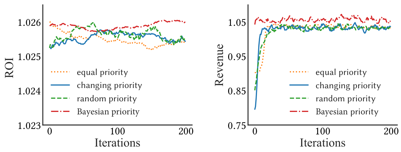
To give a comprehensive view of MoTiAC, we perform different ways to aggregate objectives. Four different variants of are considered in the experiment. Since we have two objectives, we use for the first objective and for the second:
- •
equal priority: ;
- •
changing priority: with a scalar ;
- •
random priority: ;
- •
Bayesian priority: One can refer to Eqn. (11).
As shown in Fig. 4, we present the training curves for ROI and Revenue. The first three strategies are designed before training and will not adjust to the changing environment. It turns out that they perform similarly in both objectives and could gain a decent improvement over the PID case by around +2.5% in ROI and +3% in Revenue. However, in equal priority, the curve of ROI generally drops when the iteration goes up, which stems from the fact that fixed equal weights cannot fit the dynamic environment. For changing priority, it is interesting that ROI first increases then decreases for priority shifting, as different priority leads to different optimal. In random priority, curves dramatically change in a small range since the priority function outputs the weight randomly. The Bayesian priority case, on the contrary, sets priority based on the conformity of the agent’s prior and current state. Reward partition with agent prior dominates the first three strategies by an increasingly higher ROI achievement by +2.7% and better Revenue by around +4.2%.
4.4 RQ3: Case Study
| Models | Revenue (CNY) | Cost (CNY) | ROI |
|---|---|---|---|
| PID | 0.8003 | ||
| MoTiAC | 0.8267 |
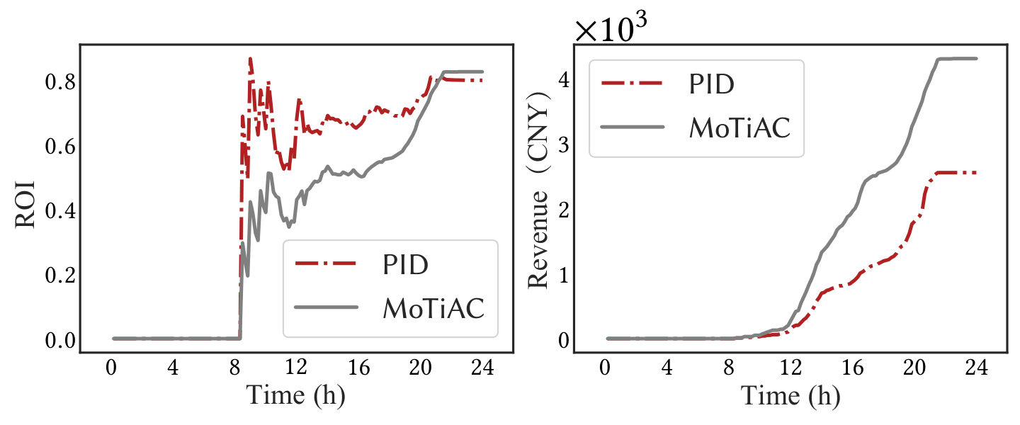
In this section, we try to investigate how MoTiAC balances the exploration of multiple objectives and achieves the optimal globally. We choose one typical ad with large conversions and show the bidding process within 24 hours. As PID is the current model in the real ad system, we use PID to compare with MoTiAC and draw the results of ROI and Revenue curve in Fig. 5. We also collect the final numerical results in Table 3.
Fig. 5 shows a pretty low ROI initially. For the target ad, both models first try to lift the ROI. Based on the figure presented on the left, the red dashed curve rises from 0 to about 0.7 sharply for PID at 8h. The potential process should be that PID has given up most of the bid chances and only concentrates on those with a high conversion rate (CVR) so that we have witnessed a low Revenue gain of the PID model in the right figure from 8h to around 21h. Though the ROI curve remains relatively low, our MoTiAC can select good impression-level chances while considering the other objective. At 24h, MoTiAC finally surpasses PID in ROI because of the high volume of pre-gained Revenue. With long-term consideration, MoTiAC beats PID on both the cumulative ROI and Revenue. We can conclude that PID is greedy out of the immediate feedback mechanism. It is always concerned with the current situation and never considers further benefits. When the current state is under control, PID will appear conservative and give a shortsighted strategy, resulting in a seemingly good ROI and poor Revenue (like the red curve in Fig. 5). However, MoTiAC has a better overall view. It foresees the long-run benefit and will keep exploration even temporarily deviating from the right direction or slowing down the rising pace (ROI curve for the target ad at 8h). Under a global overview, MoTiAC can finally reach better ROI and Revenue than PID.
5 Related Work
Real-time Bidding. Researchers have proposed static methods [15] for optimal biddings, such as constraint optimization [24], to perform an impression-level evaluation. However, traditional methods inevitably ignore that real-world situations in RTB are often dynamic [21] due to the unpredictability of user behavior [7] and different marketing plans [22] from advertisers. Furthermore, the auction process of optimal bidding is formulated as a Markov decision process (MDP) in recent study [7, 12]. Considering the various goals of different players in RTB, a robust framework is required to balance these multiple objectives. Therefore, we are motivated to propose a novel multi-objective RL model to maximize the overall utility of RTB.
Reinforcement Learning. Significant achievements have been made by the emergence of RL algorithms, such as policy gradient [19] and actor-critic [8]. With the advancement of GPU and deep learning (DL), more successfully deep RL algorithms [9, 13] have been proposed and applied to various domains. Meanwhile, there are previous attempts to address the multi-objective reinforcement learning (MORL) problem [6], where the objectives are combined mainly by static or adaptive linear weights [1, 14] or captured by a set of policies and evolving preferences [16].
6 Conclusion and Future Directions
In this paper, we propose Multi-ObjecTive Actor-Critics for real-time bidding in display advertising. MoTiAC utilizes objective-aware actor-critics to solve the problem of multi-objective bidding optimization. Our model can follow adaptive strategies in a dynamic RTB environment and outputs the optimal bidding policy by learning priors from historical data. We conduct extensive experiments on the real-world industrial dataset. Empirical results show that MoTiAC achieves state-of-the-art on the Tencent advertising dataset. One future direction could be extending multi-objective solutions with priors in the multi-agent reinforcement learning area.
References
- [1] A., A., M., D., L., T., N., A., S., D.: Dynamic weights in multi-objective deep reinforcement learning. In: International Conference on Machine Learning (ICML). pp. 11–20 (2019)
- [2] Bennett, S.: Development of the pid controller. IEEE control systems pp. 58–62 (1993)
- [3] Cai, H., Ren, K., Zhang, W., Malialis, K., Wang, J., Yu, Y., Guo, D.: Real-time bidding by reinforcement learning in display advertising. In: Proceedings of the 10th ACM International Conference on Web Search and Data Mining (WSDM). pp. 661–670 (2017)
- [4] Critch, A.: Toward negotiable reinforcement learning: shifting priorities in pareto optimal sequential decision-making. arXiv:1701.01302 (2017)
- [5] Ghavamzadeh, M., Mannor, S., Pineau, J., Tamar, A., et al.: Bayesian reinforcement learning: A survey. Foundations and Trends® in Machine Learning 8(5-6), 359–483 (2015)
- [6] Hayes, C.F., Rădulescu, R., Bargiacchi, E., Källström, J., Macfarlane, M., Reymond, M., Verstraeten, T., Zintgraf, L.M., Dazeley, R., Heintz, F., et al.: A practical guide to multi-objective reinforcement learning and planning. arXiv preprint arXiv:2103.09568 (2021)
- [7] Jin, J., Song, C., Li, H., Gai, K., Wang, J., Zhang, W.: Real-time bidding with multi-agent reinforcement learning in display advertising. In: Proceedings of the 27th ACM International Conference on Information and Knowledge Management (CIKM) (2018)
- [8] Konda, V.R., Tsitsiklis, J.N.: Actor-critic algorithms. In: Advances in Neural Information Processing Systems (NeurIPS). pp. 1008–1014 (2000)
- [9] Lillicrap, T.P., Hunt, J.J., Pritzel, A., Heess, N., Erez, T., Tassa, Y., Silver, D., Wierstra, D.: Continuous control with deep reinforcement learning. arXiv:1509.02971 (2015)
- [10] Lin, X., Zhen, H.L., Li, Z., Zhang, Q.F., Kwong, S.: Pareto multi-task learning. In: Advances in Neural Information Processing Systems (NeurIPS). pp. 12060–12070 (2019)
- [11] Lizotte, D.J., Bowling, M.H., Murphy, S.A.: Efficient reinforcement learning with multiple reward functions for randomized controlled trial analysis. In: International Conference on Machine Learning (ICML). pp. 695–702 (2010)
- [12] Lu, J., Yang, C., Gao, X., Wang, L., Li, C., Chen, G.: Reinforcement learning with sequential information clustering in real-time bidding. In: Proceedings of the 28th ACM International Conference on Information and Knowledge Management (CIKM). pp. 1633–1641 (2019)
- [13] Mnih, V., Badia, A.P., Mirza, M., Graves, A., Lillicrap, T., Harley, T., Silver, D., Kavukcuoglu, K.: Asynchronous methods for deep reinforcement learning. In: International Conference on Machine Learning (ICML). pp. 1928–1937 (2016)
- [14] Pasunuru, R., Bansal, M.: Multi-reward reinforced summarization with saliency and entailment. arXiv:1804.06451 (2018)
- [15] Perlich, C., Dalessandro, B., Hook, R., Stitelman, O., Raeder, T., Provost, F.: Bid optimizing and inventory scoring in targeted online advertising. In: Proceedings of the 18th ACM SIGKDD International Conference on Knowledge Discovery and Data Mining (KDD). pp. 804–812 (2012)
- [16] Pirotta, M., Parisi, S., Restelli, M.: Multi-objective reinforcement learning with continuous pareto frontier approximation. In: 29th AAAI Conference on Artificial Intelligence (AAAI) (2015)
- [17] Sener, O., Koltun, V.: Multi-task learning as multi-objective optimization. In: Advances in Neural Information Processing Systems (NeurIPS). pp. 525–536 (2018)
- [18] Shelton, C.R.: Balancing multiple sources of reward in reinforcement learning. In: Advances in Neural Information Processing Systems (NeurIPS). pp. 1082–1088 (2001)
- [19] Sutton, R.S., McAllester, D.A., Singh, S.P., Mansour, Y.: Policy gradient methods for reinforcement learning with function approximation. In: Advances in Neural Information Processing Systems (NeurIPS). pp. 1057–1063 (2000)
- [20] Wang, Y., Liu, J., Liu, Y., Hao, J., He, Y., Hu, J., Yan, W.P., Li, M.: Ladder: A human-level bidding agent for large-scale real-time online auctions. arXiv:1708.05565 (2017)
- [21] Wu, D., Chen, X., Yang, X., Wang, H., Tan, Q., Zhang, X., Xu, J., Gai, K.: Budget constrained bidding by model-free reinforcement learning in display advertising. In: Proceedings of the 27th ACM International Conference on Information and Knowledge Management (CIKM) (2018)
- [22] Xu, J., Lee, K.c., Li, W., Qi, H., Lu, Q.: Smart pacing for effective online ad campaign optimization. In: Proceedings of the 21th ACM SIGKDD International Conference on Knowledge Discovery and Data Mining (KDD). pp. 2217–2226 (2015)
- [23] Yuan, S., Wang, J., Zhao, X.: Real-time bidding for online advertising: measurement and analysis. In: Proceedings of the 7th International Workshop on Data Mining for Online Advertising (ADKDD). p. 3 (2013)
- [24] Zhang, W., Yuan, S., Wang, J.: Optimal real-time bidding for display advertising. In: Proceedings of the 20th ACM SIGKDD International Conference on Knowledge Discovery and Data Mining (KDD). pp. 1077–1086 (2014)
- [25] Zhao, J., Qiu, G., Guan, Z., Zhao, W., He, X.: Deep reinforcement learning for sponsored search real-time bidding. arXiv preprint arXiv:1803.00259 (2018)
- [26] Zhu, H., Jin, J., Tan, C., Pan, F., Zeng, Y., Li, H., Gai, K.: Optimized cost per click in taobao display advertising. In: Proceedings of the 23rd ACM SIGKDD International Conference on Knowledge Discovery and Data Mining (KDD). pp. 2191–2200 (2017)
Appendix 0.A Supplementary Material
0.A.1 Pricing Evaluation Metrics
We present our pricing evaluation metric below: Algorithm 2 is the pricing evaluation strategy based on our business, and in Algorithm 3 we specify the Score function.
0.A.2 Implementation Details
We shall present our implementation details for all baselines and our MoTiAC as follows:
- •
PID: control signal is given by difference across two intervals in our experiment, in order to making sure less fluctuation and stable result. Ratio for proportional factor is 0.04 , for the integral factor is 0.25 and for the derivative factor is 0.002.
- •
A2C, Agg-A3C: in A2C, we use two hidden layers with 256 and 128 dimensions. Output for Actor is one-dimension scalar and (Gaussian Distribution), and then actions will be sampled from the above-mentioned distribution with boundaries. Output for Critic is one-dimension scalar. State is a normalized 17-dimension feature vector. Agg-A3C has the same architecture, but is on extension of A2C with 5 workers running in parallel and updates global net asynchronously.
- •
DQN: all settings in DQN are the same as in A2C and Agg-A3C, except for Actor. The output of Actor has 100 dimension w.r.t 100 values ranging from 0 to 1, and 0.01 as its interval. Then based on values we choose the best , and gives as .
- •
O1-A3C, O2-A3C: all settings in O1-A3C and O2-A3C are the same as in A2C and Agg-A3C, except for reward. Reward in O1-A3C and O2-A3C is set according to their objectives.
- •
MoTiAC: we use two hidden layers with 256 and 128 dimensions for all nets in MoTiAC. However, the difference is that we have two critics in global nets with the same structures. And for each update period, one group of workers can only push their gradients to actor and one of the critics. We set 5 worker as an objective group. Also, MoTiAC is implemented with multiprocessing and shared memory.