Sampling Kaczmarz Motzkin Method for Linear Feasibility Problems: Generalization & Acceleration
Abstract
Randomized Kaczmarz (RK), Motzkin Method (MM) and Sampling Kaczmarz Motzkin (SKM) algorithms are commonly used iterative techniques for solving a system of linear inequalities (i.e., ). As linear systems of equations represent a modeling paradigm for solving many optimization problems, these randomized and iterative techniques are gaining popularity among researchers in different domains. In this work, we propose a Generalized Sampling Kaczmarz Motzkin (GSKM) method that unifies the iterative methods into a single framework. In addition to the general framework, we propose a Nesterov type acceleration scheme in the SKM method called as Probably Accelerated Sampling Kaczmarz Motzkin (PASKM). We prove the convergence theorems for both GSKM and PASKM algorithms in the norm perspective with respect to the proposed sampling distribution. Furthermore, we prove sub-linear convergence for the Cesaro average of iterates for the proposed GSKM and PASKM algorithms.From the convergence theorem of the GSKM algorithm, we find the convergence results of several well-known algorithms like the Kaczmarz method, Motzkin method and SKM algorithm. We perform thorough numerical experiments using both randomly generated and real-world (classification with support vector machine and Netlib LP) test instances to demonstrate the efficiency of the proposed methods. We compare the proposed algorithms with SKM, Interior Point Method (IPM) and Active Set Method (ASM) in terms of computation time and solution quality. In the majority of the problem instances, the proposed generalized and accelerated algorithms significantly outperform the state-of-the-art methods.
Keywords Kaczmarz Method Randomized Projection Sampling Kaczmarz Motzkin Linear Feasibility Nesterov’s Acceleration Iterative Methods
1 Introduction
We consider the following Linear Feasibility (LF) problem:
| (1) |
We confine the scope of our work in the regime of thin/tall coefficient matrix (), as iterative methods are more competitive for such problems. Note that, while almost all of the classical methods are deterministic in nature, recent advances [1, 2, 3, 4, 5, 6, 7, 8, 9, 10, 11, 12] suggest that randomized iterative methods can outperform existing deterministic methods for solving many computational problems including linear feasibility, linear systems and convex optimization problems. From an algorithmic point of view, our work generalizes the SKM method and furthermore explores the possibility of faster variants of these methods. Before we delve into the contributions of this work, we give brief descriptions of some of the classical and modern techniques related to solving LF problems with iterative methods.
Randomized Kaczmarz (RK)
Kaczmarz method is one of the popular methods for solving linear systems due to its algorithmic simplicity [13]. Originally proposed in 1937 by Kaczmarz [13], the Kaczmarz method remained hidden to the research community until the early 1980s, when Gordon et. al proposed Algebraic Reconstruction Techniques (ART) in the area of image reconstruction [14]. Later, it has found applications in several areas like computer tomography [15, 16], digital signal processing [17], distributed computing [18, 19] and many other engineering and physics problems. It has been rediscovered several times as a family of methods including component solution, successive projection, row-action and cyclic projection methods (see [20]). Given a current point , the Kaczmarz method generates new update based on the orthogonal projection of onto the hyper-plane ,
| (2) |
The differences between the old and modern Kaczmarz schemes are the choice of projection hyper-planes in the update formula of equation (2) at each iteration and the choice of projection parameter . The original Kaczmarz method chooses hyper-planes by with parameter . Strohmer et. al [1] showed that instead of using cyclic rules, convergence can be improved by choosing from at random with probability proportional to . This randomization scheme is very efficient for the linear system as well [2]. The projection parameter can be chosen any value in the range of [11].
Motzkin Method (MM)
Another classical method for solving LF problems is the Motzkin method (MM) discovered by Motzkin et. al in the early 1950s [21, 22]. The work of Motzkin was rediscovered several times by other researchers in the field of Machine Learning (ML). For instance, the so-called perceptron algorithm in ML [23, 24, 25] can be classified as a member of Motzkin type methods. Furthermore, MM can be sought as the Kaczmarz method with “maximal-residual control" or with “most violated constraint control" [20, 26, 27]. The MM starts with an initial point and finds the next update as the projection of onto the most violated hyper-plane defined in the equation (1). Given the current point , find the next projection hyper-plane as the maximum violated constraint (i.e., select ) and then update as follows
| (3) |
with the choice , where denotes the orthogonal projection of onto the hyper-plane . The analysis of the MM depends on the so-called Hoffman constant (see Lemma 3.1 and Table 1). The main drawback of the standard MM is that it fails to terminate when the LF problem of (1) is infeasible. In the late 1980s, MM resurfaced for its connection to the ellipsoid method [28]. For rational data, it’s proven that the system can detect infeasibility and for totally unimodular data, the scheme gives strong polynomial-time algorithms [29]. Recently, Chubanov [30, 31] developed a modified method compared to the traditional relaxation type methods [22], where instead of projecting on the original hyper-plane, one projects the new point to an induced hyper-plane.
In recent time, Kaczmarz type methods gained immense popularity in the research community. The work of Strohmer et. al [1] encouraged numerous extensions and variants of the RK method (see [2, 3, 5, 6, 7, 8, 32]). For instance, in [5, 33], authors analyzed variants of the Kaczmarz method for a least square setup. A significant breakthrough came from the work of Gower et. al when they developed a generalized framework namely the Gower-Richtarik (GR) sketch. The authors showed that several well-known algorithms like Randomized Kaczmarz (RK), Randomized Newton (RN) and Randomized Coordinate Descent methods can be sought as special cases of the GR algorithm. For different choices of sampling distribution and a positive definite matrix, one can recover all of the above algorithms as special cases (see [8, 34, 10, 35] for a detailed discussion).
Another area of research spurred when Gower et. al provided the extension of the GR sketching method to combine several Quasi-Newton methods into one framework [36]. They showed that almost all of the available Quasi-Newton algorithms like Bad Broyden (BB), Powell-Symmetric-Broyden (PSB), Good Broyden (GB), Broyden–Fletcher–Goldfarb–Shanno (BFGS) and Davidon–Fletcher–Powell (DFP) can be derived as special cases of the GR sketch. In another work, they extended the GR method for finding the pseudo-inverse of a matrix [37]. Several variants of acceleration have been explored recently for the GR sketch [38, 39]. Special block variants of RK methods have been analyzed by Needell et. al [40, 41, 42]. From a linear programming perspective, Chubanov developed a polynomial-time algorithm for solving the linear system [30, 43, 44] and LF problem [31]. In recent time, other variants of both RK and SKM algorithms have been developed that deal with various types of sampling strategies [45, 46, 10, 47, 48].
Moreover, a large number of scientific computing and machine learning tasks aim to solve the unconstrained minimization problem with a differentiable function [49]. Gradient Descent (GD) and its variants have been the de facto choice in the artificial intelligence and machine learning community to solve such problems [50]. However, GD suffers from slow convergence as soon as the current solution approaches . To achieve faster convergence, one of the major algorithmic development is the idea of momentum. The momentum method was first studied by Polyak [51] in the sense of rolling a heavy ball along with a well-defined cost function. However, despite its intuitiveness, Polyak’s heavy ball momentum was difficult to analyze mathematically. Nesterov’s acceleration method, proposed by Nesterov in his seminal work [52] for the GD provides the mathematical rigor that Polyak’s method lacks and exhibits the worst-case convergence rate of for minimizing smooth convex functions compared to the original convergence rate of . Since the introduction of Nesterov’s work, numerous work has been done on algorithmic development of the first-order accelerated methods (for a detailed discussion see [53, 54, 55, 56]). From then on, Nesterov and Polyak’s work has been integrated into several well-known projection-based algorithms like Coordinate Descent [56], Randomized Kaczmarz [32], Momentum Induced GR Sketching [57], Affine Scaling [58], Accelerated Quasi-Newton [39], Randomized Gossip [59], Sampling Kaczmarz Motzkin [60] and the references therein. Particularly, Morshed et. al [60] investigated the acceleration scheme of Nesterov in the SKM algorithm for .
In this work, we develop a generalized framework namely the GSKM method that extends the SKM algorithm and proves the existence of a family of SKM type methods for solving LF problems. This general framework will provide an ideal platform for the researchers to experiment with a wide range of iterative projection methods and to design efficient algorithms for solving optimization problems in areas like artificial intelligence, machine learning, data mining, and engineering. In addition to the general framework, we propose a Nesterov type acceleration scheme in the SKM method () that outperforms state-of-the-art methods in terms of computation time and solution quality. With the convergence analysis of the GSKM algorithm, we synthesize the convergence analysis of SKM type methods into one convergence theorem from which one can derive convergence results of RK, MM and SKM methods. We also prove convergence of the average iterate (i.e., Cesaro average) generated by both GSKM and PASKM method. We prove sub-linear convergence rate for the Cesaro average under somewhat weaker conditions. We carry out thorough numerical experiments to show the effectiveness of the proposed methods in comparison with state-of-the-art methods for solving a wide range of linear feasibility test instances. Although the proposed methods deal with the case of linear feasibility problem with systems of inequalities, it can be noted that with some modification, like the one stated in the work of Lewis et. al [2], one can apply this method to linear systems with both equality and inequality constraints.
The remainder of the paper is organized as follows. The proposed algorithms are discussed in section 2, and the convergence analysis of the proposed algorithms is given in section 3. In section 4, we perform extensive numerical experiments on artificial and real test instances for a better understanding of the behavior of the proposed generalized and accelerated schemes. Besides, we compared the effectiveness of the proposed acceleration schemes with state-of-the-art techniques (i.e., SKM, IPM and ASM). And finally, the paper is concluded in section 5 with concluding remarks and future research directions.
2 Preliminaries & Contributions
In this section, we discuss the SKM algorithm and some preliminary technical tools to analyze the SKM type methods. We first discuss the notations and assumptions that will be used throughout the paper. We then briefly discuss the SKM method along with the expectation induced by the sampling distribution of the SKM method. To make the analysis easier and more formal, we introduce the function . Finally, we conclude the section with the proposed GSKM method and the PASKM method and their geometric interpretations.
2.1 Notation
We follow the standard linear algebra notation in this work. denotes the dimensional real space, denotes the set of real-valued matrices. For any matrix , denotes the transpose matrix and for denotes the rows of matrix . Furthermore, denotes the feasible region of the feasibility problem and denotes the projection of onto the feasible region . The notation denotes the distance between and the feasible region , i.e., . For any matrix , the spectral norm and Frobenius norm are denoted by and , respectively. For any function , we use to represent the gradient of . Finally, denotes the standard inner product and as the euclidean () norm. The notation denotes the positive part of any real number (ie., ). For any two arbitrary matrices , the notation implies the positive definiteness of the matrix . The notation is used to denote the expectation with respect to the sampling distribution .
2.2 Assumptions
Throughout the paper, we assume that the system is consistent and the matrix has no zero rows. We also assumed that the rows of matrix are normalized (i.e., for all ). Note that, normalization simplifies the convergence analysis considerably. The normalization doesn’t impact the computational time significantly (we could simply normalize each row for the first time it occurs during the computation). Moreover, normalization simplifies the convergence analysis considerably. In the description of algorithms, we do not enforce the assumption. Furthermore, it can be noted that the proposed algorithms generate the same iterates irrespective of normalization.
2.3 Sampling Kaczmarz Motzkin
The SKM method (Algorithm 1) for solving LF problems, proposed by De Loera et. al [11], combines the ideas of both Kaczmarz and Motzkin method. The authors provided a generalized convergence Theorem and a certificate of feasibility which synthesizes the convergence analysis of the Kaczmarz method and Motzkin method for solving LF problems. The proposed method requires only memory storage and is much more efficient than the state-of-the-art techniques such as Kaczmarz type methods, IPMs and ASMs. The main advantage of SKM can be ascribed to its innovative way of projection plane selection. The hyper-plane selection goes as follows: at iteration the SKM algorithm selects a collection of rows namely uniformly at random out of rows of the constraint matrix , then out of these rows the row with maximum positive residual is selected (i.e., choose row as ) and finally the next point is updated as follows
| (4) |
For ease of analysis, we denote the above sampling distribution as at iteration , i.e., at each iteration choose and denote as .
The SKM method generalizes RK and MM, and it also combines their strength in choosing a constraint at each iteration. It has a cheaper per iteration cost compared to Motzkin’s method and converges faster compared to the Kaczmarz method. Several extensions of the SKM method in terms of acceleration [60], improved rate [61] have been proposed recently.
2.4 Expectation
For the convergence analysis of Algorithm 1 and its variations (any algorithm that uses that specific type of sampling distribution), we need to discuss a specific expectation calculation. First of all, let us sort the residual vector from smallest to largest for any iterate and denote as the entry on the sorted list 11 1 We use the notation throughout the paper to express the underlying expectation, where the indices represent the sampling process of 5., i.e.,
| (5) |
Now, consider the list with all of the entries of the residual vector , then we need to calculate the probability that particular entry of the residual vector is selected at any given iteration. Note that, the probability that any sample is selected is and each sample has an equal probability of selection. Another intersecting fact can be noted that the size of the residual list controls the order and frequency that each entry of the residual vector will be expected to be selected. From now on, we will denote this specific choice of sampling distribution as for any point 22 2 For ease of notation, throughout the paper, we will use to denote the sampling distribution corresponding to any random iterate . To calculate the resulting expectation with respect to the above-mentioned sampling distribution, let us first denote, as the set of sampled constraints and as 33 3 Similarly, we will use to denote the sampled set and for any iterate .
| (6) |
where, denotes the collection of rows of restricted to the index set and denotes the entry of . Using the above discussion with the list provided in equation (5), we have the following:
| (7) |
where, denotes the required expectation corresponding to the sampling distribution . The above expectation calculation was first used by De Loera et.al in their work [11] where they first introduced the SKM method.
2.5 Function
In this section, we formalize the definition of function . Throughout section 3, we will use the properties of function 44 4 Similar type of functions with uniform sampling have been studied in [10] [12] in the context of stochastic gradient descent and alternating projection algorithms respectively.. First, for any index , let us define the following function
| (8) |
Then to simplify the expectation expression of (7) further, we define the function and the gradient of as follows:
| (9) |
where, the index is selected by the rule provided in (6).
2.6 Contributions
Generalized Sampling Kaczmarz Method (GSKM). For obtaining a generalized version of the SKM method, we suggest using history information in updating the current update. In particular, we take two random iterates and generated by successive SKM iteration and then update the next iterate as an affine combination of the previous two updates. Starting with , for , we update
where is the update of the SKM algorithm. Note that, by taking , one can recover the original SKM algorithm. For simpler representation, we denote this method as a generalized SKM method or GSKM method. GSKM method is formally provided in Algorithm 2 and the convergence analysis is provided in subsection 3.2. Our convergence analysis suggests that for any , one could choose any such that 55 5 see (3.2)..
| (10) | ||||
| (11) |
|
|
Convergence Rate | Algorithm | |||
|---|---|---|---|---|---|---|
|
|
|
RK [1] | ||||
|
|
|
MM [22] | ||||
|
|
|
SKM [11] |
In Table 1, we list the algorithms and their respective convergence Theorems recovered from the GSKM algorithm with different parameter choices. To simplify the notation, we denote, .
Probably Accelerated Sampling Kaczmarz Method (PASKM). We propose an accelerated randomized projection method based on the SKM method and Nesterov accelerated gradient (NAG). Note that, NAG generates sequences and using the following update formulas:
| (12) |
In equation (2.6), is the gradient of the given function and are the step sequences. Nesterov used updated values for the sequences and obtained a better convergence rate for the acceleration of standard gradient descent. There are two available works directly involve applying Nesterov’s acceleration in Kaczmarz type methods 66 6 Recently, heavy ball momentum method has been proposed in the context of SKM method [62], first one is by Wright et. al [32] where the accelerated RK method is proposed for linear systems, the second one deals with applying acceleration in SKM for [60].
In this work, we consider the general case and develop a probably accelerated scheme for the SKM algorithm. The main difference between the proposed PASKM algorithm and the above-mentioned method is the choice of step sequences. We propose to use precomputed values for the parameters for every iterate compared to the iterative parameter selection process in [56, 32, 60]. Now, using the definition of function (see (8)) in (2.6), we derive the following scheme:
| (16) |
with chosen as , where . The PASKM method is formalized as Algorithm 3 and the detailed convergence analysis of the method is provided in Section 3. This method generally outperforms both the SKM and GSKM algorithms for almost all of the test instances considered in this work (see Section 4).
2.7 Geometric Interpretation
The goal of this section is to provide a geometric interpretation of the proposed GSKM and PASKM methods. We shed more lights on how the proposed algorithms work in practice and the difference among SKM, GSKM and PASKM methods.


In Figures 1 and 2, we illustrate the differences among SKM, GSKM and PASKM methods in an plane. Our goal is to show how each of the proposed algorithms progress at each iteration. For illustration purposes, We performed the experiment with only two hyper-planes and the selection of hyper-planes is done in an alternative fashion. The notation denotes the orthogonal projection of point onto the hyper-plane . For comparison purposes, we started with the same starting point and drew the figures with the same scaling. For any given starting point , each algorithm projects the point onto the most violated constraint from the sampled constraint set.
The projection step corresponds to the computation of the term , which means that the current update is projected onto the violated hyper-plane. The projection parameter defines the type of projection. When , the projection is exact, that is the point belongs to the hyper-plane . GSKM can be seen as a kind of convex projection update which is slower compared to SKM. From Figure 2, it can be seen that the GSKM method with proceeds faster compared to SKM and it requires an affine combination of the previous two successive projections (i.e., and ). Compared to SKM and GSKM, the PASKM method updates three different sequences . From Figure 2, it can be noted that GSKM with negative and PASKM moves faster to the feasible region compared to the SKM method (later in the numerical section this comparison will become much more apparent for larger test instances).
2.8 Connection between GSKM and PASKM
Assume, . Then, we can simplify the update formula of the GSKM method as
| (17) |
where the indices and are selected following the rule of (8) for the iterate and , respectively. Furthermore, take and such that the condition holds, then from the update formula of the PASKM method we get,
Similarly, from the definition of , we have
| (18) |
where the indices and are selected following the rule of (8) for the iterate and , respectively. Considering update formulas (17) and (2.8), we can conclude that if the conditions and hold, then the sequence generated by the GSKM algorithm and the sequence generated by the PASKM algorithm is the same sequence.
3 Main Results
In this section, we present the convergence analysis of the proposed algorithms. In the first subsection, we provided the necessary technical Lemmas Theorems that will be used later for our convergence analysis. In the second subsection, we provided the convergence Theorems of the GASKM algorithm. Finally, the last subsection deals with the convergence analysis of the PASKM method.
3.1 Technical Tools
In this subsection, we will discuss two types of results. Most of the results derived are related to the properties of the function . Lemma 3.1 is the famous result of Hoffman regarding the linear system of inequalities. Lemmas 3.6-3.9 discuss the strong convexity and existence of Lipschitz constant along some restricted segment. Finally, Theorems 3.12 and 3.13 deal with developing decay bounds for some non-negative sequences. We will use Lemmas 3.6-3.9 frequently in our convergence analysis. Theorems 3.12 and 3.13 will be used to derive the proposed convergence bounds of the quantities and .
Lemma 3.1.
(Hoffman [63], Theorem 4.4 in [2]) Let and be the feasible region, then there exists a constant such that the following identity holds:The constant is the so-called Hoffman constant. Note that, for a consistent system of equations (i.e., there exists a unique such that ), can be expressed in terms of the smallest singular value of matrix , i.e.,
Lemma 3.2.
(Lemma 2.1 in [11]) Let be real non-negative sequences such that and , thenLemma 3.3.
For any and , the following identity holds,Lemma 3.4.
Let be the eigenvalue of the matrix , then for all , the bound holds.Proof.
Since is positive semi-definite, we can write for all . Also as the mapping is convex, using Jensen’s inequality we have,
∎
Lemma 3.5.
For any , we have the following:Proof.
See Appendix 1. ∎
Lemma 3.6.
For any with , we have the following: with .Proof.
See Appendix 1. ∎
Lemma 3.6 states that the function is strongly convex with constant and has Lipschitz continuous gradient with constant when restricted along the segment . Let, , then it can be easily checked that . Here, is the optimal solution and it satisfies . Moreover, the point satisfies the condition . Then we rewrite the inequalities of Lemma 3.6 as follows
| (19) | ||||
| (20) |
Here, equation (19) and (20) represent the Lipschitz continuity condition and the strong convexity condition respectively along the line segment . For our convergence analysis of Algorithm 2 and 3, we will need inequalities like (19) and (20) along the segment for any . Following two Lemmas deal with the problem of finding such bounds.
Lemma 3.7.
For any , we have the following:Proof.
See Appendix 1. ∎
Remark 3.8.
We note that the condition of Lemma 3.7 is weaker than the traditional strong convexity, and it is also weaker than the essentially strong convexity condition defined in [64]. For instance, the essentially strong convexity requires the following identity:
for some . The above condition clearly implies (33). Moreover, the restricted secant inequality condition defined in [64] can be written as
| (21) |
Note that, with the choice in Lemma 3.7, we have the following:
Here, we used the fact . This implies that the function satisfies the restricted secant inequality condition of (21) with constant . Indeed it can be shown that the constant can be improved further (see the following Lemma).
Lemma 3.9.
For any and such that , we have the following:Proof.
See Appendix 1. ∎
Remark 3.10.
Substituting , in Lemma 3.9 we have,
Note that, similar types of results can be found in the literature. For instance, in [12], authors obtained similar result with respect to a different expectation, they used for any , which is commonly used to analyze randomized Kaczmarz type methods (see [1, 2]). Furthermore, we believe a better upper bound than the one obtained in Lemma 3.7 can be obtained considering some restrictions on the data matrix . To that end, one needs to obtain a better version of equation (33), i.e., one needs to show that the function is convex along the line segment .
Lemma 3.11.
For any and , we have the following: where, , and .Proof.
See Appendix 1. ∎
Before we delved into the main Theorems, for any , let us define the following parameters:
| (22) |
The following two Theorems deal with the growth of non-negative real sequences. We will use these results in our main analysis of GSKM and PASKM method.
Theorem 3.12.
Let be a non-negative real sequence satisfying the following relation: if and then the following bounds hold: 1. (Lemma 9 in [57]) Let, be the largest root of , then 2. Define , then we have the following: where, and .Proof.
See Appendix 1. ∎
Theorem 3.13.
Let the real sequences and satisfy the following recurrence relation: (23) where, such that the following relations (24) hold. Then the sequence and converges and the following result holds: where, (25) and and .Proof.
See Appendix 1. ∎
3.2 Convergence Analysis of the GSKM Method
In this subsection, we study convergence properties of the proposed GSKM method, i.e., we study the convergence behavior of the quantities of and . For any , let us define the sets as
| (26) |
We proved that whenever and , the proposed GSKM method enjoys a global linear rate. We also provided convergence analysis of the function values (i.e., ) with respect to the Cesaro average. Our results are global in nature and to the best of our knowledge, this is the first of its kind result for the SKM method.
Theorem 3.14.
Let be the sequence of random iterates generated by algorithm 2. With the choice of parameters, and , the sequence of iterates converges and the following results hold: 1. Take and as in equation (3.1), then 2. Take and , then where, the constants are defined in equation (3.1) and and . 3. Also the average iterate for all satisfies the followingProof.
See Appendix 2.
∎
In the above Theorem, we obtain a global linear rate for the GSKM method with . Note that, when , we have,
Since the maximum value of can be derived as , the above inequality attains equality when (see the next Corollary). This gives us . Since the rate of the SKM algorithm is given by , we can say that the theoretical convergence rate of Algorithm 2 is always worse or equal compared to SKM whenever .
Corollary 3.14.1.
(Theorem 1.3 in [11]) Let be the sequence of random iterates generated by the SKM method (algorithm 1) starting with . With , the sequence of iterates converges and the following result holds:Proof.
Note that, if we let in the GSKM method, then we have , which is precisely the SKM method. Now, take in Theorem 3.14, then considering the first part of the Theorem, we have . Furthermore, from the second part, we have . This proves the result of Corollary 3.14.1 which is precisely the convergence rate obtained in [11] for the SKM method. ∎
Our next Theorem, states that, for a range of negative values of the parameter , the GSKM method enjoys a global linear rate.
Theorem 3.15.
Let be the sequence of random iterates generated by algorithm 2 and let and . Define (27) and as in (24) with the parameter choice of (27). Then the sequence of iterates converges and the following result holds: where and .Proof.
See Appendix 2. ∎
Parameter Choice for GSKM
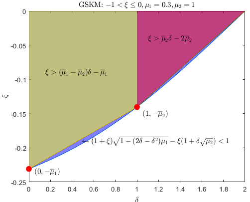
From Theorem 3.14, it can be noted that the GASKM method will converge for any . Whenever is negative (i.e., ), the allowable range for can be shown in the following figure. In Figure 3, we plot the feasible region for allowable values for . Denote, and . Then the feasible region of Figure 3 can be approximated piece-wise as for and for . Moreover, any pair that resides inside the region also resides inside the feasible region of Theorem 3.15.
Cesaro Average:
In the next Theorem, we propose the convergence analysis of the function values , with respect to the Cesaro average. Instead of bounding in terms of initial function value , we bound the decay in terms of a larger quantity that results in a better convergence rate. To the best of our knowledge, this is the first result that shows convergence of the Kaczmarz type methods for solving linear feasibility problems 77 7 Several works exits for the Kaczmarz type methods for solving linear systems [38, 57].. An interesting corollary of our method is the Cesaro average result for the SKM method. Furthermore, the result holds under weaker assumptions than the previous Theorems.
Theorem 3.16.
Let be the random sequence generated by Algorithm 2. Take, and . Define and as in (9), thenProof.
See Appendix. ∎
Corollary 3.16.1.
Let be the random sequence generated by SKM method (algorithm 1). Define and as in (9), then holds for any .Proof.
Take in Theorem 3.16, then the result follows. ∎
The next Theorem is an extension of the result obtained in [11] and to a certain extent, it can be taken as an extension of Telgen’s result [28]. The Theorem gives one a certificate of feasibility after a finite number of GSKM iterations. Before delving into the Theorem, we will provide some known Lemmas for the SKM algorithm which holds for the GSKM algorithm too. We refer interested readers to the work of De-Loera et. al [11] for detailed proof of these Lemmas (Lemma 3.17 to Lemma 3.19).
Lemma 3.17.
(Lemma 1 in [11]) Define, as the maximum violation of point and the length of the binary encoding of a linear feasibility problem with rational data-points as Then if the rational system is infeasible, for any , the maximum violation satisfies the following lower bound:Lemma 3.18.
(Lemma 4 in [11]) If is -dimensional (full-dimensional) then the sequence of iterates generated by the GSKM method converges to a point .Proof.
Since, by assumption, is full dimensional, then the rest of the proof follows the same argument as Lemma 4 in [11]. ∎
Lemma 3.19.
([65]) If the rational system is feasible, then there is a feasible solution whose coordinates satisfy for .Certificate of feasibility:
To detect feasibility of the rational system , one needs to find a point such that . Such a point if exists will be called a certificate of feasibility. When the system is feasible, one expects to find a certificate of feasibility after finitely many iterations, and that if one fails to find a certificate after finitely many iterations, one can obtain a lower bound on the probability that the system is infeasible. Moreover, as discussed in the next Theorem, if the system is feasible, one can bound the probability of finding a certificate of feasibility.
Theorem 3.20.
Suppose are rational matrices with binary encoding length, , and that we run the GSKM method (, ) on the system with . Suppose the number of iterations satisfies the following lower bound: If the system is feasible, then, where is the probability that the current iterate is not a certificate of feasibility. And , where and are defined in Theorem 3.14 and Theorem 3.15 for the choice and , respectively. Also note that the function is a decreasing function with respect to .Proof.
See Appendix.
∎
Remark 3.21.
Note that instead of a normalized system if we consider a non-normalized system for some , then suppose the number of iterations satisfies the following lower bound:
where is the binary encoding length for . If the system is feasible, then,
where probability that the current update is not a certificate of feasibility and .
Corollary 3.21.1.
(Theorem 1.5 in [11]) Suppose are rational matrices with binary encoding length, , and that we run the SKM method on the system for some and . Suppose the number of iterations satisfies the following lower bound: where is the binary encoding length for . If the system is feasible, then, where the probability that the current update is not a certificate of feasibility and .3.3 Convergence Analysis of the PASKM Method
In this subsection, we study convergence properties of the proposed PASKM algorithm, i.e., we study the convergence behavior of the quantities of , , and generated by the PASKM method. We proved that for a range of step parameters , the proposed PASKM method enjoys a global linear rate. We also provided convergence analysis of the function values , with respect to the Cesaro average. The next Theorem deals with the convergence of the sequences and as well as the function values generated by the PASKM algorithm.
Theorem 3.22.
Let be the sequence of random iterates generated by algorithm 3 and let and such that , and the following condition (28) holds. Define, , and as in (24). Then the sequence of iterates and converges and the following results hold: and where and .Proof.
See Appendix 3. ∎
The next Theorem deals with the convergence of the sequences and generated by the PASKM algorithm.
Theorem 3.23.
Let, and are generated by Algorithm 3. If we select the parameters as where, is chosen as if , otherwise choose any . Then, for any , the sequence of iterates converges and the following result holds: This theorem implies that the PASKM algorithm converges linearly with a rate of , which accumulates to a total of iterations to bring the given error below .Proof.
See Appendix 3. ∎
In the next Theorem, we present the convergence analysis of the function with respect to the Cesaro average for the PASKM algorithm. We showed that the Cesaro average of the PASKM iterates converges to the optimum at a rate of where is the number of iterations.
Theorem 3.24.
Let be the random sequence generated by Algorithm 3. Take, , and . Define and as in (9), thenProof.
See Appendix 3. ∎
Parameter selection for PASKM algorithm
In this section, we discuss allowable parameter selection for the PASKM algorithm based on Theorem 3.22. If the parameters and satisfies and the condition of (3.22) hold then the PASKM method will converge for any 88 8 When, , we have . In that case, we can simplify the condition of (3.22) as . In other words, for the PASKM algorithm will converge if we select the parameters as , , and .. To simplify the conditions for ease of implementation, let’s take and for some 99 9 Note that for the choice the condition (3.3) trivially holds as the right hand side of (3.3) is always greater than ..
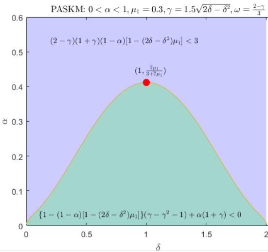
In Figure 4, we plot the feasible region considering the above parameter choice and the conditions of Theorem 3.22. Considering the choice of and , the condition simplifies to
where, we used the fact that the conditions and hold for any . That implies for any , the condition holds. Similarly, we can simplify the condition of (3.22) as follows:
| (29) |
Therefore, if we choose and as
| (30) | ||||
| (31) |
then the convergence result of Theorem 3.22 holds for the PASKM algorithm. We will use these two sets of parameter choices in our numerical experiments. Note that, our choice is empirical in nature. One can probably find a better combination of parameters than (30) and (31). Similarly, if we choose and as
| (32) |
then the convergence result of Theorem 3.23 holds for the PASKM algorithm. The choice of (32) is not of practical benefit as the value of is very small for most test cases. From (32), we have , which is very small for large test instances. Smaller slows down the convergence of the PASKM algorithm as can be seen as a projection parameter like .
4 Numerical Experiments
In this section, we discuss the numerical experiments performed to show the computational efficiency of the proposed algorithms (Algorithm 2 and 3). As mentioned before, we limit our focus on the over-determined systems regime (i.e., ) where iterative methods are competitive in general. However, from our experiments, we see similar computational behavior for the under-determined systems as well.
4.1 Experiment Specifications
We implemented the proposed GSKM and PASKM algorithms in MATLAB R2018b and performed the experiments in a Dell Precision 7510 workstation with 32GB RAM, Intel Core i7-6820HQ CPU, processor running at 2.70 GHz. To analyze computational performance, we perform the numerical experiments for a wide range of instances including both randomly generated and real-world test problems.
- •
Randomly generated problems: Gaussian and highly correlated systems
- •
Real-world test instances: Standard ML data sets and Sparse Netlib LP instances
We compare SKM with two versions of the proposed GSKM and PASKM algorithms for a better understanding of the algorithmic behavior. In Table 2, we provide the parameter choices for GSKM and PASKM algorithms. Throughout the numerical experiments section, we compared SKM with GSKM-1, GSKM-2 and PASKM-1, PASKM-2.
| Parameters |
|
| |||||||||
|---|---|---|---|---|---|---|---|---|---|---|---|
|
|
|
|
| |||||||
|
|
|
|
| ||||||||
Finally, we investigate the performance behavior of the proposed GSKM and PASKM methods with state-of-the-art methods such as Interior point methods (IPMs) and Active set methods (ASMs) for several Netlib LP instances. The total CPU time is calculated in seconds (s). For a fair comparison, we run the algorithms 10 times and report the averaged performance throughout the experiments. Moreover, all the algorithms start from the same initial point that is far away from the feasible region.
4.2 Experiments on Randomly Generated Instances
We considered the linear feasibility , where the entries of matrices and are chosen randomly from a certain distribution. To maintain the system consistency (i.e., ), we first generated vectors at random from the corresponding distributions, then set as the convex combination of vectors and (i.e., ). Two types of random data sets are considered: highly correlated, and Gaussian. For the correlated systems, data matrices and are chosen uniformly at random between (i.e., ). For the Gaussian system data matrices, and are chosen uniformly at random from standard normal distribution (i.e., ). Moreover, the vector is generated by following the above-mentioned procedure.
CPU time vs Sample size
We first compared the total CPU time of the proposed algorithms (GSKM-1, GSKM-2, PASKM-2, PASKM-2) with the original SKM algorithm. The comparison is carried out by varying the sample size from to the total row size . The positive residual error tolerance is chosen as (i.e., ). The comparison is carried out for and . In Figure 5, we compared the above-mentioned algorithms for two randomly generated highly correlated linear feasibility problems of size and . From Figure 5, we see that the proposed GSKM-1, PASKM-1, PASKM-2 algorithms outperform the SKM algorithm in terms of average CPU time when . For , the performance of SKM, PASKM-1 and PASKM-2 are fairly similar whereas, the performance of GSKM-1 and GSKM-2 are worse compared to all other algorithms.


We present the time versus sample size plot for two randomly generated Gaussian system of size and in Figure 6. All the algorithms show similar performance patterns as shown in the correlated systems (Figure 5) for the choice of . However, for the case of , SKM and PASKM-2 perform marginally better than the other algorithms. Since all of the considered methods perform significantly well whenever is small (i.e., ). For a better understanding, we compare the proposed algorithms for . In Figure 7, we plot the time vs graph for a Gaussian problem for smaller .

In a nutshell, we can conclude that for the choice of , PASKM-1, PASKM-2 and GSKM-1 outperform the original SKM method. And in that region, PASKM-2 is the best performing algorithm. Moreover, for , all of the proposed algorithms perform similarly as the SKM method. However, for the case of , the proposed algorithms significantly outperform the SKM method. Furthermore, we believe with correct parameter choice one can find better-performing variants of GSKM and PASKM compared to the SKM algorithm for the case of . Finally from Figure 7, we can deduce that the best sample size choice for all of the considered methods occurs at . This amplifies the importance of the special sampling distribution selection.
Positive residual error VS No. of iterations and Time
Now, we compare the respective convergence trend for the considered algorithms with respect to the number of iterations and CPU time.

We choose positive residual error as the convergence measure and considered Gaussian system. We carried out the analysis for several choices of sample sizes, and the choice of values remains the same as before. In Figures 8 and 9, we provide the respective positive residual decay results for different sample sizes and different projection parameters. We plot positive residual error VS iteration and positive residual error VS time in Figures 8 and 9, respectively. From Figures 8 and 9, we see that irrespective of sample size, converges to zero much faster for the proposed PASKM-1 and PASKM-2, GSKM-1 compared to SKM whenever . For the case of , SKM and PASKM-2 has a similar kind of performance whereas the GSKM-1 performs poorly compared to SKM and PASKM method. As expected, the choice produces the slowest rate and the choice produces the best convergence graph.

Fraction of satisfied constraints (FSC) VS No. of iterations and Time
To investigate the generated solution quality of the above-mentioned algorithms of Table 2, we measure the number of satisfied constraints at each iteration, for that we define,
Note that, at any particular iteration we have, .

In Figures 10 and 11, we plot the value of FSC with respect to No. of iterations and CPU time of each algorithm respectively. From Figures 10 and 11, we can see that the choice of is the worst choice for all algorithms as the improvement of FSC is much slower compared to other choices of . And for the choice , we get the best solution quality for each algorithm. Our proposed GSKM-1, PASKM-1 and PASKM-2 algorithms outperform the other methods significantly for but, for only PASKM-2 performs similar to SKM.

4.3 Experiments on real-world Instances
In this subsection, we consider some nonrandom, real-world test instances. For the sake of unbiased performance analysis, we consider the following two types of real-world data-sets: standard Machine Learning (ML) data-sets for Support Vector Machine (SVM) classifier [66, 67, 11], and sparse linear feasibility problems extracted from benchmark Netlib LP problems [68].
SVM classifier instances
We first consider two linear feasibility problems arising from binary classification with SVM. We compare the proposed algorithms with SKM to the linear classification problem using the SVM model for the following two data sets: 1) Wisconsin (diagnostic) breast cancer data set and 2) Credit card default data set. The Wisconsin breast cancer data set consists of data points whose features are calculated from images. There are two types of data points: 1) malignant and 2) benign cancer cells. As shown by the researchers [69, 11], the SVM classifier problem can be re-written as an equivalent homogeneous system of linear inequalities (), which represents the separating hyper-plane between malignant and benign data points. The constraint matrix has rows (data points) and columns (features). Since the data set is not perfectly separable, we allow tolerance for the positive residual . For our experiments, we fixed the tolerance as (i.e., we ran the algorithm until is satisfied).
Similarly, we consider the credit card default data set described in [66, 11]. This data set consists of features denoting the payment profile of a user and binary variables describing payment conditions in a certain billing cycle: 1 for payment made on time and 0 for late payment. The SVM classification problem for the data set can be transformed into an equivalent homogeneous system of inequalities () like before. The solution denotes the coefficients of the separating hyper-plane between on-time and default data points. The transformed data matrix has rows ( user profiles) and columns ( profile features). As the data set is not separable, like the previous problem we allow a tolerance error. In this case, we ran the algorithms until the condition: is satisfied.
CPU time vs Sample size
We plot the CPU time VS sample size graphs for SVM problems in Figure 12. To be consistent with our previous experiments, we choose . From Figure 12, we see that the proposed GSKM-1, PASKM-1 and PASKM-2 algorithms outperform the other algorithms including SKM for . However, for , GSKM-2 performs significantly well compared to the other methods. On the other hand, SKM, PASKM-1 and PASKM-2 follow a similar trend across different sample sizes. PASKM-1 and PASKM-2 marginally outperform SKM for this regime. Another interesting point can be noted that the comparison graphs for the credit card data set are not as smooth as the breast cancer data set graphs 1010 10 The credit card data matrix has rows. From our earlier experiments, we observe that the choice of , the proposed algorithms produce the best performance. For that reason, we plot the credit card graph up-to . The irregularity of the credit card graph occurs when ., which can be attributed to the irregularity of the constraint matrix .

Netlib LP instances
We also investigate the comparative performance of the proposed algorithms with SKM on real-world sparse data sets. For this experiment, we consider some Netlib LP [68] test instances. Each of these problems is formulated as a standard linear programming problem ( subject to ). To conduct the above-mentioned experiments, we transform each of these problems into an equivalent linear feasibility problem.
CPU time vs Sample size
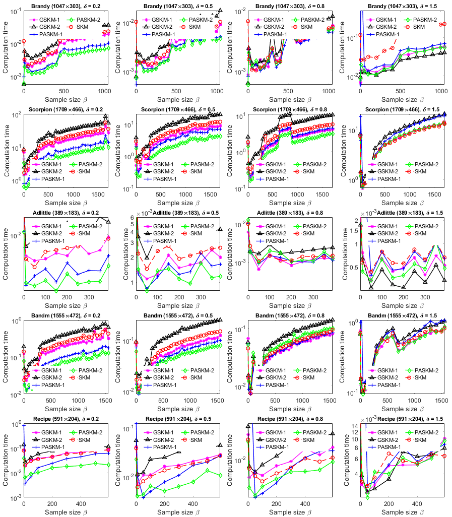
Now, we plot the CPU time VS sample size graphs for five Netlib LP instances in Figure 13. Later in subsection 4.4, we consider a total of ten Netlib LP instances including the five considered here. In Figure 13, we provide comparison graphs for the following Netlib LP test instances: lp-brandy, lp-addlittle, lp-scorpion, lp-bandm, lp-recipe. Furthermore, we consider different error tolerances for these problems (see Table 3 for details). From Figure 13, we see that the proposed GSKM-1, PASKM-1, PASKM-2 algorithms outperform the SKM algorithm for . In the case of , the performance of SKM, GSKM-1 and PASKM-2 are fairly similar for the problems lp-scorpion, lp-bandm and lp-recipe. For lp-brandy and lp-adlittle, all of the proposed variants of GSKM and PASKM outperform the original SKM.
4.4 Comparison with IPM and ASM for Netlib LP instances
In this subsection, we compare the performance of GSKM and PASKM variants with SKM and benchmark commercial solvers for solving Netlib LP test instances. We follow the standard framework used by De Loera et. al [11] and Morshed et. al [60] in their work for linear feasibility problems. The problem instances are transformed from standard LP problems (i.e., subject to with optimum value ) to an equivalent linear feasibility formulation (i.e.,, where and ). For all of the experiments, we compared the proposed algorithms for , since from our experiments in subsection 4.2 and 4.3, this is the domain where the proposed GSKM and PASKM variants significantly outperform the SKM method.
In Table 3, we list the total CPU time in seconds for each of the above-mentioned algorithms in Table 2. In addition to that, we provide the CPU time for Interior point method (IPM) and Active set method (ASM) algorithms for solving the selected Netlib LP problems. For a better and fair comparison, the pseudo-code of the proposed methods and SKM is written in MATLAB and Optimization Toolbox function fmincon is used to implement IPM and ASM methods. We first solve the linear feasibility problem () with SKM, GSKM and PASKM variants and record the CPU time in Table 3. Note that, we can’t use fmincon’s IPM and ASM algorithms directly to solve the linear feasibility problem () since both methods fail to solve the linear feasibility problems. The reason for that is, in IPM the Karush Kuhn Tucker (KKT) system at each iteration becomes singular, and ASM stops in the first step of finding a feasible solution.
Instance Dimensions GSKM PASKM SKM Interior Point Active set adlittle 0.027 0.173 0.032 2.16 4.96 150 0.1 agg 0.22 0.196 0.23 50 1 bandm 9.82 4.057 9.2 14.57 50 1 blend 1.48 0.581 1.28 2.28 4.62 50 0.1 brandy 0.53 0.491 14.06 16.97 63.11 1 1 degen2 26.26 10.139 20.73 7.13 21038 100 1 finnis 0.53 0.532 0.527 10 0.1 recipe 0.60 0.164 0.52 0.89 63.24 50 0.1 scorpion 156.9 42.712 125 17.68 8.02 50 1 stocfor1 1.05 0.553 0.95 2.13 2.52 50 0.1
For a fair comparison, in Table 3, we list the total CPU consumption time as follows: for the SKM method we solve the feasibility problem () for a certain and 1111 11 we note the best possible time from our previous experiments, for GSKM and PASKM variants we solve the same feasibility problem and report the best performing method from each of the two, and finally for fmincon algorithms, we use the original LPs (). Note that, this is not an ideal or obvious comparison, for a better suitable comparison we follow the framework used in [11, 60]. We set the stopping criterion for SKM, GSKM and PASKM variants as and the halting criterion for the fmincon’s algorithms (IPM, ASM) are set as and , where is the tolerance gap listed in Table 3. To avoid any biased conclusion, for each problem we set the initial update as far as possible from the feasible region.
From the comparison in Table 3, we can see that the proposed algorithms work much faster than IPM and ASM but work marginally better than the existing SKM method. Notice that the improvement of PASKM and GSKM algorithms over the SKM method for most problems are marginal as the proposed algorithms are designed explicitly for dense matrices. One can develop special algorithmic variants of the proposed PASKM and GSKM methods for sparse problems by following some standard aggregation techniques. A possible technique is to combine multiple steps by using the sparsity of the test instances. For instance, after iteration when we have and , instead of moving forward with the sequences and , for any we can skip iterations and update and using a generalized recurrence relation that can enhance the computational efficiency.
5 Conclusion
In this work, we propose a general algorithmic framework (GSKM) for solving linear feasibility problems that unify various SKM type algorithms with the addition of a relaxation parameter . From our convergence analysis of the GSKM method, one can recover convergence Theorems of several well-known algorithms such as Randomized Kaczmarz, Motzkin Method and Sampling Kaczmarz Motzkin method. In addition to the general framework, we propose a Nesterov type acceleration scheme in the SKM method called as PASKM. Our proposed PASKM method provides a bridge between Nesterov type acceleration of Machine Learning to sampling Kaczmarz methods for solving linear feasibility problems. To show the effectiveness of the proposed algorithms, we performed a wide range of numerical experiments on various types of random and standard benchmark data sets. For a better understanding of the behavior of the proposed algorithms, we numerically analyze two variants for both GSKM and PASKM algorithms in comparison with the original SKM method. Furthermore, we compare our proposed methods to commercially available methods such as IPM and ASM. In the majority of the test instances, the proposed algorithms significantly outperform the state-of-the-art methods. Furthermore, as shown in our numerical experiments, the correct choice of parameters can lead to much faster and accelerated methods for different types of test instances.
Future Research
In the future, the proposed algorithms and the technical analysis can be adopted effectively to various types of extensions such as sparse variants, optimally tuned PASKM, and GSKM, PASKM variants with greedy sampling strategies. First, we plan to extend our work to design efficient sparse variations of the proposed methods that can handle large-scale real-world problems with greater sparsity in the data matrix . Second, we intend to design a test instance dependent scheme for identifying optimal parameter selection (i.e., , , , , ) for both GSKM and PASKM. For the GSKM algorithm, adaptive parameter selection (i.e., , , ) policy can be a great area of future research. One can also derive connecting ideas between the proposed GSKM and induced projection plane generation of Chubanov [30, 31] which can produce faster algorithms. Finally, we aspire to develop adaptive sampling strategies and integrate the greedy Kaczmarz [48] type method into the GSKM framework to further speed up the convergence.
6 Acknowledgements
The authors are truly grateful to the anonymous referees and the editors for their valuable comments and suggestions in the earlier version of the paper. The comments helped immensely in the revision process and greatly improved the quality of this paper.
Appendix 1
Proof of Lemma 3.5
Proof of Lemma 3.6
Using the definition of the expectation from (7), we have,
Here, is the number of zero entries in the residual , which also corresponds to the number of satisfied constraints for . Since , we have the following:
Combining the above identities and using the expression for from (9) we get,
which proves the Lemma.
Proof of Lemma 3.7
From the definition of , it can be easily checked that is a convex function. Now, by the convexity property of , for any , we have the following:
| (33) |
Therefore, we have
This completes the proof.
Proof of Lemma 3.9
Since, , from the definition we have,
Here, we used the identity . This proves the Lemma.
Proof of Lemma 3.11
Proof of Theorem 3.12
Since, , the largest root of equation can written as
Then using the given recurrence we have,
This proves the first part. Also note that since , we have,
For the second part, notice that from the recurrence inequality, we can deduce the following matrix inequality:
| (34) |
The Jordan decomposition of the matrix in the above expression is given by,
| (35) |
Next, we discuss two possible cases of values of . Also, we substituted in the Jordan decomposition of equation (35).
Case 1: even
| (36) |
Here, we used .
Case 2: odd
| (37) |
Here, we used the inequality . Now combining the relations from equation (Case 1: even) and (Case 2: odd), we can prove the second part of Theorem 3.12.
Proof of Theorem 3.13
From the given recurrence relation, we have
| (38) |
Using the definitions of (3.13), we can write the Jordan decomposition of the above matrix as follows
| (39) |
Now, substituting the matrix decomposition into equation (38) and simplifying we have
| (40) |
Since , one can easily verify that . Now, it remains to show that . To show that, first note that
| (41) |
Now, we have,
Moreover, since , we have
As , considering (Proof of Theorem ) we can deduce that the sequence and converges.
Appendix 2
Proof of Theorem 3.14
From the update formula of Algorithm 2, we have where,
| (42) |
Similarly, the previous update formula can be written as, ; where,
| (43) |
Note that, the notation is consistent with the definition of (6). Since for any , we have,
| (44) |
We used the fact that the function is convex and . Now, taking expectation in both sides of the equation (44) and using Lemma 3.11, we get the following:
| (45) |
where, is defined in Lemma 3.11. Taking expectation again in equation (Proof of Theorem ) and letting , we get the following:
| (46) |
Since, , and , using first part of Theorem 3.12, we have the following:
| (47) |
Moreover, considering (47) with Lemma 3.6 we get the bound of which proves the first part of Theorem 3.14. Furthermore, using the second part of Theorem 3.12 and equation (46), we get the second part of Theorem 3.14. Now, to prove the third part first note that , using Lemma 3.3 we have
| (48) |
Furthermore, using a more simplifies version of (44) we have the following:
for any . Summing up the above identity for , we have the following:
| (49) |
where, . We used the non-negativity of the sequences and . We also used the upper bound from Lemma 3.6. Then, we get
This proves the second part of Theorem 3.14.
Proof of Theorem 3.16
For any natural number define, , and , then using the update formulas (10) and (11), we have
here, the index and are defined based on (6) respectively for the sequences and . Using the above relation, we can write
| (50) |
Taking expectation with respect to we have,
| (51) |
Similarly, we can simplify the third term of (Proof of Theorem ) as
| (52) |
Using the expressions of equation (51) and (Proof of Theorem ) in (Proof of Theorem ) and simplifying further, we have
| (53) |
here,
| (54) |
Now, taking expectation again in (53) and using the tower property, we get,
| (55) |
where, . Summing up (55) for we get
| (56) |
Now, using Jensen’s inequality, we have
Since, , we have . Furthermore,
| (57) |
Now, from our construction we get
Substituting the values of and in the expression of , we have the following:
Proof of Theorem 3.15
Since, the term is constant under From the update formula of the GSKM algorithm, we get,
| (58) |
We performed the two expectations in order, from the innermost to the outermost. Now, taking expectation in (Proof of Theorem ) and using the tower property of expectation we have,
| (59) |
Similarly, using the update formula for , we have
| (60) |
Taking expectation in (Proof of Theorem ) and using (59) along with the tower property, we have,
| (61) |
Combining both (59) and (Proof of Theorem ), we can deduce the following matrix inequality:
| (62) |
Now, from the definition, it can be easily checked that . Since, , we have
| (63) |
Also, we have
| (64) |
Here, in the last inequality we used the given condition. Considering (64), we can check that . Also from (63), we have , which is precisely the condition provided in (24). Let’s define the sequences and . Now, using Theorem 3.13, we have
| (65) |
where, can be derived from (3.13) using the parameter choice of (27). Note that, from the GSKM algorithm we have, and .Therefore we can easily check that, and . Now, substituting the values of and in (65), we have
| (66) |
Also from Theorem 3.13 we have, and . Which proves the Theorem.
Proof of Theorem 3.20
Note that, since is feasible, then from Lemma 3.19, we know that there is a feasible solution with for . Thus, we have,
| (67) |
as . Then if the system is infeasible, by using Lemma 3.17, we have,
This implies when GSKM runs on the system , the system is feasible when . Furthermore, since every point of the feasible region is inside the half-space defined by for all , we have the following:
| (68) |
Then, for whenever the system is feasible, we have,
| (69) |
Similarly for whenever the system is feasible, we have,
| (70) |
Take, 1212 12 Note that, since and , from Theorem 3.15 we have for any .. Now combining (69) and (70), for any , whenever the system is feasible, we have,
| (71) |
Here, we used Theorems 3.14 & 3.15 and the identities from equations (67) & (68). Now, for detecting feasibility we need to have, . That gives us,
Simplifying the above identity further we get the following lower bound for :
Moreover, if the system is feasible, then the probability of not having a certificate of feasibility is bounded as follows,
Here, we used the Markov’s inequality . This completes the proof of Theorem 3.20.
Appendix 3
Proof of Theorem 3.22
From the update formula of the PASKM algorithm, we get,
| (72) |
Here, we used the condition . Similarly, using the update formula for , we have
| (73) |
Following Theorem 3.13, let us define the sequences and . The goal is to prove that and satisfy the condition (24). Now, taking expectation in (Proof of Theorem ) and using the tower property of expectation we have,
| (74) |
Similarly, taking expectation in (Proof of Theorem ) and using (74) along with the tower property of expectation we have,
| (75) |
Combining both (74) and (Proof of Theorem ), we can deduce the following matrix inequality:
| (76) |
Here, we use the fact that . Now we will use Theorem 3.13 to simplify the expression of (76). Before we can use Theorem 3.13, we need to make sure the sequences and satisfy the condition of (24). From the definition, we have
| (77) |
Also, we have
| (78) |
Here, in the last inequality, we used the given condition. Considering (Proof of Theorem ), we can check that . Also from (Proof of Theorem ), we have , which is precisely the condition provided in (24). Now, using Theorem 3.13, we have
| (79) |
where, can be derived from (3.13) using the given parameter. Note that, from the PASKM algorithm we have, . Therefore we can easily check that, . Now, substituting the values of and in (79), we have
| (80) |
Also from Theorem 3.13 we have, and . Which proves the the first part of the Theorem. Now, considering Lemma 3.6, we get
| (81) |
Now, substituting the result of (80) in (81), we get the second part of the Theorem.
Proof of Theorem 3.23
Let us define, . Since , using the update formula of from equation (15), we have,
| (82) |
Since is a convex function and , we can bound the expected first term as follows,
| (83) |
Taking expectation with respect to the sampling distribution in the second term of equation (Proof of Theorem ) and using Lemma 3.11 with the choice and , we get,
| (84) |
Now, taking expectation in the third term of (Proof of Theorem ) we get,
| (85) |
Using Lemma 3.7 and Lemma 3.9 we can simplify equation (Proof of Theorem ) as follows,
| (86) |
Now, substituting the values of equation (Proof of Theorem ), (Proof of Theorem ) & (Proof of Theorem ) in equation (Proof of Theorem ) we get the following:
With further simplification, the above identity can be written as follows:
| (87) |
Now, let’s choose the parameters as in equation (32) along with . We can easily see that and . Also note that,
| (88) |
which implies . Similarly, whenever we have
| (89) |
which implies . Also, using the parameter choice of (32), we have,
| (90) |
Now, using all of the above relations (equation (32), (Proof of Theorem )) in equation (Proof of Theorem ), we get the following:
| (91) |
Finally, taking expectation again with tower rule and substituting we have,
This proves the Theorem. Furthermore, for faster convergence, we need to choose parameters such that, becomes as small as possible. In the proof, we assumed holds which is the most probable scenario. Whenever , we must have and Lemma 6 holds with both equality, i.e., . Therefore if we choose as , we can check that condition (89) holds and holds for any .
Proof of Theorem 3.24
For any natural number , using the update formula of , we have
| (92) |
Let . It can be easily checked that . Now, considering equation (13), we have
| (93) |
here, the index and are defined based on (6) respectively for the sequences and . Furthermore, with the choice of , the points and generated by the PASKM method (i.e, algorithm 3 with arbitrary parameter choice) can be calculated as
| (94) |
since . Now, let’s define, , and , then using the update formula (Proof of Theorem ), we have
Using the above relation, we can write
| (95) |
Taking expectation with respect to we have,
| (96) |
Similarly, we can simplify the third term of (Proof of Theorem ) as
| (97) |
Using the expressions of equation (96) and (Proof of Theorem ) in (Proof of Theorem ) and simplifying further, we have
| (98) |
here,
| (99) |
Now, taking expectation again in (98) and using the tower property, we get,
| (100) |
where, . Summing up (100) for we get
| (101) |
Now, using Jensen’s inequality, we have
From (Proof of Theorem ), and . Then,
| (102) |
Now, from our construction we get
Substituting the values of and in the expression of , we have the following:
References
- [1] Thomas Strohmer and Roman Vershynin. A randomized kaczmarz algorithm with exponential convergence. Journal of Fourier Analysis and Applications, 15(2):262, Apr 2008.
- [2] Dennis Leventhal and Adrian S. Lewis. Randomized methods for linear constraints: Convergence rates and conditioning. Mathematics of Operations Research, 35(3):641–654, 2010.
- [3] Deanna Needell. Randomized kaczmarz solver for noisy linear systems. BIT Numerical Mathematics, 50(2):395–403, Jun 2010.
- [4] Petros Drineas, Michael W. Mahoney, Shan Muthukrishnan, and Tamás Sarlós. Faster least squares approximation. Numerische Mathematik, 117(2):219–249, Feb 2011.
- [5] Anastasios Zouzias and Nikolaos M. Freris. Randomized extended kaczmarz for solving least squares. SIAM Journal on Matrix Analysis and Applications, 34(2):773–793, 2013.
- [6] Yin Tat Lee and Aaron Sidford. Efficient accelerated coordinate descent methods and faster algorithms for solving linear systems. In Proceedings of the 2013 IEEE 54th Annual Symposium on Foundations of Computer Science, FOCS ’13, pages 147–156, Washington, DC, USA, 2013. IEEE Computer Society.
- [7] Anna Ma, Deanna Needell, and Aaditya Ramdas. Convergence properties of the randomized extended gauss seidel and kaczmarz methods. SIAM Journal on Matrix Analysis and Applications, 36(4):1590–1604, Jan 2015.
- [8] Robert M. Gower and Peter Richtárik. Randomized iterative methods for linear systems. SIAM Journal on Matrix Analysis and Applications, 36(4):1660–1690, 2015.
- [9] Zheng Qu, Peter Richtarik, Martin Takac, and Olivier Fercoq. SDNA: Stochastic Dual Newton Ascent for Empirical Risk Minimization. In Proceedings of The 33rd International Conference on Machine Learning, volume 48, pages 1823–1832, New York, USA, 20–22 Jun 2016. PMLR.
- [10] Deanna Needell, Nathan Srebro, and Rachel Ward. Stochastic gradient descent, weighted sampling, and the randomized kaczmarz algorithm. Mathematical Programming, 155(1):549–573, Jan 2016.
- [11] Jesús De Loera, Jamie Haddock, and Deanna Needell. A sampling kaczmarz–motzkin algorithm for linear feasibility. SIAM Journal on Scientific Computing, 39(5):S66–S87, 2017.
- [12] Meisam Razaviyayn, Mingyi Hong, Navid Reyhanian, and Zhi-Quan Luo. A linearly convergent doubly stochastic gauss–seidel algorithm for solving linear equations and a certain class of over-parameterized optimization problems. Mathematical Programming, 176(1):465–496, Jul 2019.
- [13] Stefan Kaczmarz. Angenaherte auflsung von systemen linearer gleichungen. Bulletin International de l’Acadmie Polonaise des Sciences et des Letters, 35:355–357, 1937.
- [14] Richard Gordon, Robert Bender, and Gabor T. Herman. Algebraic reconstruction techniques (art) for three-dimensional electron microscopy and x-ray photography. Journal of Theoretical Biology, 29(3):471 – 481, 1970.
- [15] Yair Censor. Parallel application of block-iterative methods in medical imaging and radiation therapy. Mathematical Programming, 42(1):307–325, Apr 1988.
- [16] Gabor T. Herman. Fundamentals of Computerized Tomography: Image Reconstruction from Projections. Springer Publishing Company, Incorporated, 2nd edition, 2009.
- [17] D. A. Lorenz, S. Wenger, F. Schöpfer, and M. Magnor. A sparse kaczmarz solver and a linearized bregman method for online compressed sensing. In 2014 IEEE International Conference on Image Processing (ICIP), pages 1347–1351, Oct 2014.
- [18] Joseph M. Elble, Nikolaos V. Sahinidis, and Panagiotis Vouzis. Gpu computing with kaczmarz’s and other iterative algorithms for linear systems. Parallel Computing, 36(5):215 – 231, 2010. Parallel Matrix Algorithms and Applications.
- [19] Fabio Pasqualetti, Ruggero Carli, and Francesco Bullo. Distributed estimation via iterative projections with application to power network monitoring. Automatica, 48(5):747 – 758, 2012.
- [20] Yair Censor. Row-action methods for huge and sparse systems and their applications. SIAM Review, 23(4):444–466, 1981.
- [21] Shmuel Agamon. The relaxation method for linear inequalities. Canadian J. Math, pages 382–392, 1954.
- [22] Theodore S. Motzkin and Issac J. Schoenberg. The relaxation method for linear inequalities. Canadian J. Math, pages 393–404, 1954.
- [23] Frank Rosenblatt. The perceptron: A probabilistic model for information storage and organization in the brain. Psychological Review, pages 65–386, 1958.
- [24] Aaditya Ramdas and Javier Peña. Margins, kernels and non-linear smoothed perceptrons. In Proceedings of the 31st International Conference on Machine Learning, volume 32, pages 244–252, Bejing, China, 22–24 Jun 2014. PMLR.
- [25] Aaditya Ramdas and Javier Peña. Towards a deeper geometric, analytic and algorithmic understanding of margins. Optimization Methods and Software, 31(2):377–391, 2016.
- [26] Julie Nutini, Behrooz Sepehry, Issam Laradji, Mark Schmidt, Hoyt Koepke, and Alim Virani. Convergence rates for greedy kaczmarz algorithms, and faster randomized kaczmarz rules using the orthogonality graph. In Proceedings of the Thirty-Second Conference on Uncertainty in Artificial Intelligence, UAI’16, pages 547–556, Arlington, Virginia, United States, 2016. AUAI Press.
- [27] Stefania Petra and Constantin Popa. Single projection kaczmarz extended algorithms. Numerical Algorithms, 73(3):791–806, Nov 2016.
- [28] Jan Telgen. On relaxation methods for systems of linear inequalities. European Journal of Operational Research, 9(2):184 – 189, 1982.
- [29] J. F. Maurras, K. Truemper, and M. Akgül. Polynomial algorithms for a class of linear programs. Mathematical Programming, 21(1):121–136, Dec 1981.
- [30] Sergei Chubanov. A strongly polynomial algorithm for linear systems having a binary solution. Mathematical Programming, 134(2):533–570, Sep 2012.
- [31] Sergei Chubanov. A polynomial projection algorithm for linear feasibility problems. Mathematical Programming, 153(2):687–713, Nov 2015.
- [32] Ji Liu and Stephen J. Wright. An accelerated randomized kaczmarz algorithm. Math. Comput., 85(297):153–178, 2016.
- [33] Deanna Needell, Ran Zhao, and Anastasios Zouzias. Randomized block kaczmarz method with projection for solving least squares. Linear Algebra and its Applications, 484:322 – 343, 2015.
- [34] Anna. Ma, Deanna. Needell, and Aaditya. Ramdas. Convergence properties of the randomized extended gauss–seidel and kaczmarz methods. SIAM Journal on Matrix Analysis and Applications, 36(4):1590–1604, 2015.
- [35] Ahmed. Hefny, Deanna. Needell, and Aaditya. Ramdas. Rows versus columns: Randomized kaczmarz or gauss–seidel for ridge regression. SIAM Journal on Scientific Computing, 39(5):S528–S542, 2017.
- [36] Robert M. Gower and Peter Richtárik. Linearly convergent randomized iterative methods for computing the pseudoinverse, 2016.
- [37] Robert M. Gower and Peter. Richtárik. Randomized quasi-newton updates are linearly convergent matrix inversion algorithms. SIAM Journal on Matrix Analysis and Applications, 38(4):1380–1409, 2017.
- [38] Peter Richtárik and Martin Takáč. Stochastic reformulations of linear systems: Algorithms and convergence theory, 2017.
- [39] Robert Gower, Filip Hanzely, Peter Richtarik, and Sebastian U Stich. Accelerated stochastic matrix inversion: General theory and speeding up bfgs rules for faster second-order optimization. In S. Bengio, H. Wallach, H. Larochelle, K. Grauman, N. Cesa-Bianchi, and R. Garnett, editors, Advances in Neural Information Processing Systems 31, pages 1619–1629. Curran Associates, Inc., 2018.
- [40] Deanna Needell and Joel A. Tropp. Paved with good intentions: Analysis of a randomized block kaczmarz method. Linear Algebra and its Applications, 441:199 – 221, 2014. Special Issue on Sparse Approximate Solution of Linear Systems.
- [41] Jonathan Briskman and Deanna Needell. Block kaczmarz method with inequalities. J. Math. Imaging Vis., 52(3):385–396, July 2015.
- [42] Deanna Needell and Elizaveta Rebrova. On block gaussian sketching for the kaczmarz method, 2019.
- [43] Amitabh Basu, Jesús A. De Loera, and Mark Junod. On chubanov’s method for linear programming. INFORMS Journal on Computing, 26(2):336–350, 2014.
- [44] László A. Végh and Giacomo Zambelli. A polynomial projection-type algorithm for linear programming. Operations Research Letters, 42(1):91 – 96, 2014.
- [45] Yonina C. Eldar and Deanna Needell. Acceleration of randomized kaczmarz method via the johnson–lindenstrauss lemma. Numerical Algorithms, 58(2):163–177, Oct 2011.
- [46] A. Agaskar, C. Wang, and Y. M. Lu. Randomized kaczmarz algorithms: Exact mse analysis and optimal sampling probabilities. In 2014 IEEE Global Conference on Signal and Information Processing (GlobalSIP), pages 389–393, Dec 2014.
- [47] Zhong-Zhi Bai and Wen-Ting Wu. On relaxed greedy randomized kaczmarz methods for solving large sparse linear systems. Applied Mathematics Letters, 83:21 – 26, 2018.
- [48] Zhong-Zhi. Bai and Wen-Ting. Wu. On greedy randomized kaczmarz method for solving large sparse linear systems. SIAM Journal on Scientific Computing, 40(1):A592–A606, 2018.
- [49] Nikola B Kovachki and Andrew M Stuart. Analysis of momentum methods. arXiv preprint arXiv:1906.04285, 2019.
- [50] Sebastian Ruder. An overview of gradient descent optimization algorithms. arXiv preprint arXiv:1609.04747, 2016.
- [51] Boris T Polyak. Some methods of speeding up the convergence of iteration methods. USSR Computational Mathematics and Mathematical Physics, 4(5):1–17, 1964.
- [52] Yuri Nesterov. A method for solving the convex programming problem with convergence rate . Soviet Mathematics Doklady, Vol. 27:p(372–376), 1983.
- [53] Yuri Nesterov. Smooth minimization of non-smooth functions. Mathematical Programming, 103(1):127–152, May 2005.
- [54] Yuri Nesterov. Gradient methods for minimizing composite functions. Mathematical Programming, 140(1):125–161, Aug 2013.
- [55] Yuri Nesterov. Introductory Lectures on Convex Optimization: A Basic Course. Springer Publishing Company, Incorporated, 1 edition, 2014.
- [56] Yuri Nesterov. Efficiency of coordinate descent methods on huge-scale optimization problems. SIAM Journal on Optimization, 22(2):341–362, 2012.
- [57] Nicolas Loizou and Peter Richtárik. Momentum and stochastic momentum for stochastic gradient, newton, proximal point and subspace descent methods, 2017.
- [58] Md Sarowar Morshed and Md. Noor-E-Alam. Generalized affine scaling algorithms for linear programming problems. Computers & Operations Research, 114:104807, 2020.
- [59] Michael Rabbat Nicolas Loizou and Peter Richtárik. Provably accelerated randomized gossip algorithms. Arxiv, 2018.
- [60] Md Sarowar Morshed, Md Saiful Islam, and Md. Noor-E-Alam. Accelerated sampling kaczmarz motzkin algorithm for the linear feasibility problem. Journal of Global Optimization, Oct 2019.
- [61] Jamie Haddock and Anna Ma. Greed works: An improved analysis of sampling kaczmarz-motkzin, 2019.
- [62] Md Sarowar Morshed and Md. Noor-E-Alam. Heavy ball momentum induced sampling kaczmarz motzkin methods for linear feasibility problems. arXiv preprint arXiv:200908251, 2020.
- [63] Alan J Hoffman. On approximate solutions of systems of linear inequalities. In Selected Papers Of Alan J Hoffman: With Commentary, pages 174–176. World Scientific, 2003.
- [64] Hamed Karimi, Julie Nutini, and Mark Schmidt. Linear convergence of gradient and proximal-gradient methods under the polyak-łojasiewicz condition. In Paolo Frasconi, Niels Landwehr, Giuseppe Manco, and Jilles Vreeken, editors, Machine Learning and Knowledge Discovery in Databases, pages 795–811, Cham, 2016. Springer International Publishing.
- [65] L.G. Khachiyan. Polynomial algorithms in linear programming. USSR Computational Mathematics and Mathematical Physics, 20(1):53 – 72, 1980.
- [66] I-Cheng Yeh and Che-hui Lien. The comparisons of data mining techniques for the predictive accuracy of probability of default of credit card clients. Expert Syst. Appl., 36(2):2473–2480, Mar 2009.
- [67] Moshe Lichman. UCI machine learning repository, 2013.
- [68] Netlib. The netlib linear programming library.
- [69] Giuseppe Calafiore and Laurent El Ghaoui. Optimization Models. Control systems and optimization series. Cambridge University Press, October 2014.