A Stein Goodness-of-fit Test for Directional Distributions

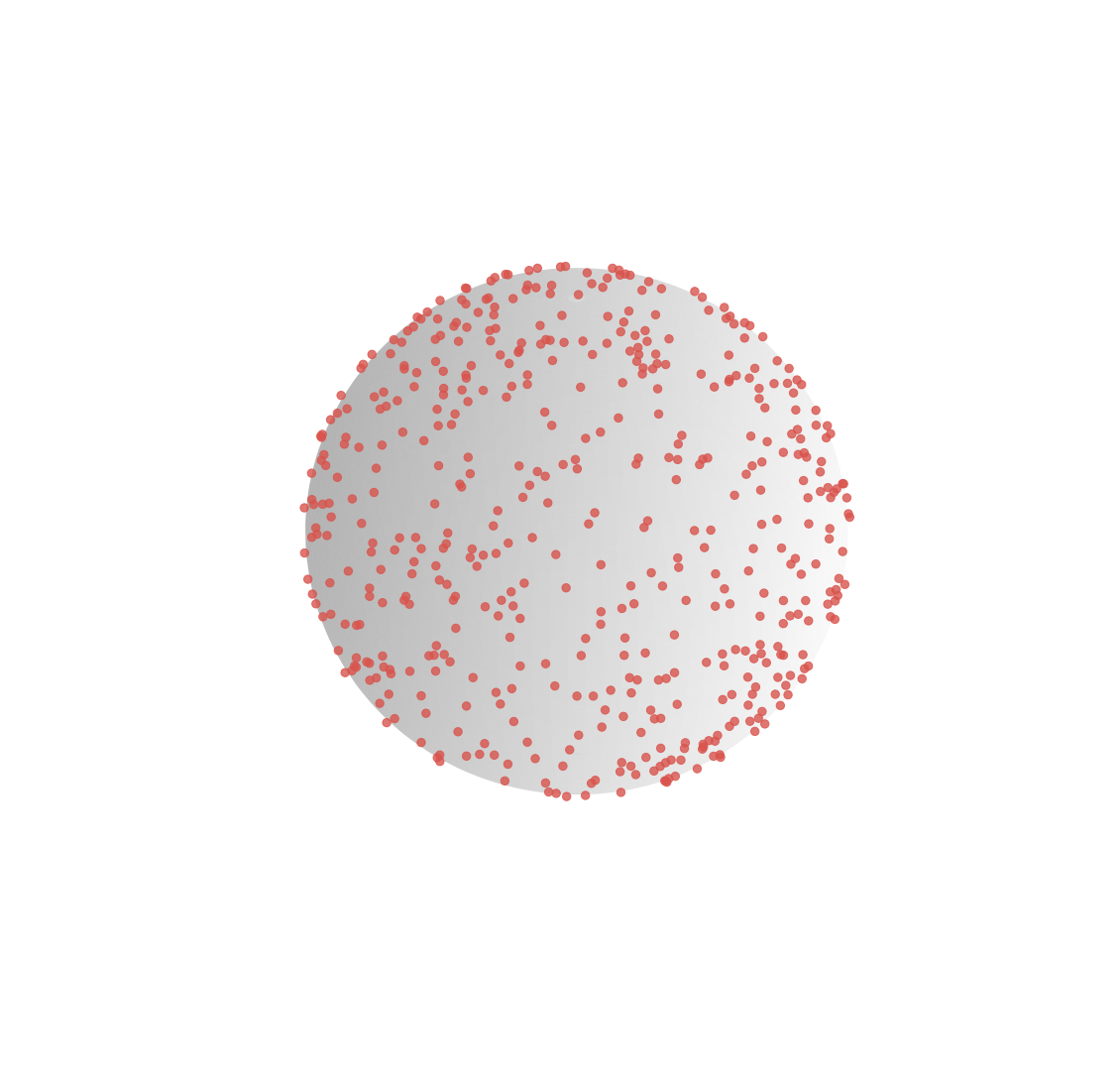
Several distributions have been proposed for describing directional data on the unit hypersphere $\mathcal{S}^{d-1}=\{x\in\mathbb{R}^{d}\mid\|x\|=1\}$. Here, we present two representative directional distributions: von Mises-Fisher and Fisher-Bingham. Figure 1 shows samples from these distributions on $\mathcal{S}^{2}$. See [37] for more detail.

In this paper, we define the probability density of directional distributions by taking the uniform distribution on $\mathcal{S}^{d-1}$ as base measure. Namely, the density of the uniform distribution is $p(x)\equiv 1$.

The von Mises-Fisher (or von Mises when $d=2$) distribution is a directional counterpart of the isotropic Gaussian distribution on $\mathbb{R}^{d}$. Its density is given by

for $x\in\mathcal{S}^{d-1}$, where $\mu\in\mathcal{S}^{d-1}$, $\kappa>0$,

and $I_{v}$ is the modified Bessel function of the first kind and order $v$. It is a unimodal distribution with peak at $\mu$ and degree of concentration specified by $\kappa$.

The Fisher-Bingham (or Kent) distribution is an extension of the von Mises-Fisher distribution [30]. Its density is given by

for $x\in\mathcal{S}^{d-1}$, where $A\in\mathbb{R}^{d\times d}$ is symmetric and $b\in\mathbb{R}^{d}$. The normalization constant $Z(A,b)$ is not represented in closed form in general.

The goodness-of-fit test for general directional distributions is not well established, to the best of our knowledge. Tests for specific distributions such as uniform [10, 15, 37] and von Mises-Fisher [11, 36] cannot be readily extended to general directional distributions. Although [5] proposed testing procedures based on the kernel density estimator, they are difficult to apply to unnormalized models such as the Fisher-Bingham distribution (2), because they require the normalization constant of the null model to calculate the $L^{p}$ test statistics.

Here, we briefly review the goodness-of-fit testing with kernel Stein discrepancy on $\mathbb{R}^{d}$ by [8, 35], which is inspired from [18, 33]. See [8, 35] for more detail.

Let $q$ be a smooth probability density on $\mathbb{R}^{d}$. For a smooth function $f=(f_{1},\dots,f_{d}):\mathbb{R}^{d}\to\mathbb{R}^{d}$, Stein’s operator $\mathcal{T}_{q}$ is defined by

From integration by parts on $\mathbb{R}^{d}$, we obtain the equality

under mild regularity conditions. Since Stein’s operator $\mathcal{T}_{q}$ depends on the density $q$ only through the derivatives of $\log q$, it does not involve the normalization constant of $q$, which is a useful property for dealing with unnormalized models [24].

Let $\mathcal{H}$ be a reproducing kernel Hilbert space (RKHS) on $\mathbb{R}^{d}$ and $\mathcal{H}^{d}$ be its product. By using Stein’s operator, kernel Stein discrepancy (KSD) [8, 35] between two densities $p$ and $q$ is defined as

It is shown that $\mathrm{KSD}(p,q)\geq 0$ and $\mathrm{KSD}(p,q)=0$ if and only if $p=q$ under mild regularity conditions [8]. Thus, KSD is a proper discrepancy measure between densities. After some calculation, $\mathrm{KSD}(p,q)$ is rewritten as

where $h_{q}$ does not involve $p$.

Now, suppose we have samples $x_{1},\dots,x_{n}$ from unknown density $p$ on $\mathbb{R}^{d}$. Based on (5), estimates of $\mathrm{KSD}^{2}(p,q)$ are obtained by using U-statistics or V-statistics. These estimates can be used to test the hypothesis $H_{0}:p=q$. The critical value is determined by bootstrap based on the theory of U-statistics or V-statistics. In this way, a general method of goodness-of-fit test on $\mathbb{R}^{d}$ is obtained, which is applicable to unnormalized models as well.

The original derivation of Stein’s operator for distributions on $\mathbb{R}^{d}$ was based on integration by parts, in which the boundary term vanishes due to the decaying property of the probability density. We need a different argument for spheres because its topology is different from $\mathbb{R}^{d}$. Specifically, differential forms and Stokes’ theorem are essential to discuss integration by parts on spheres. Here, we briefly review these concepts. See [12, 39] for more detail and rigorous treatments.

Let $M$ be a $d$-dimensional closed manifold and take its local coordinate system $x^{1},\dots,x^{d}$. We introduce symbols ${\rm d}x^{1},\dots,{\rm d}x^{d}$ and an associative and anti-symmetric operation $\wedge$ between them called the wedge product: ${\rm d}x^{i}\wedge{\rm d}x^{j}=-{\rm d}x^{j}\wedge{\rm d}x^{i}$. Note that ${\rm d}x^{i}\wedge{\rm d}x^{i}=0$. Then, a $p$-form $\omega$ on $M$ ($0\leq p\leq d$) is defined as

where the sum is taken over all $p$-tuples $\{i_{1},\cdots,i_{p}\}\subset\{1,\dots,d\}$ and each $f_{i_{1}\cdots i_{p}}$ is a smooth function on $M$. The exterior derivative ${\rm d}\omega$ of $\omega$ is defined as the $(p+1)$-form given by

For another coordinate system $y^{1},\dots,y^{d}$ on $M$, the differential form is transformed by

The integration of a $d$-form on a $d$-dimensional manifold is naturally defined like the usual integration on $\mathbb{R}^{d}$ and invariant with respect to the coordinate selection. Correspondingly, the integration by parts formula on $\mathbb{R}^{d}$ is generalized in the form of Stokes’ theorem.

In particular, since $\partial\mathcal{S}^{d-1}$ is empty, we obtain the following.

Corollary 1 plays an important role in the derivation of Stein’s operator on $\mathcal{S}^{d-1}$.

In this paper, we use the spherical coordinate system $\theta=(\theta^{1},\dots,\theta^{d-1})$ on $\mathcal{S}^{d-1}$ defined by

where $(\theta^{1},\dots,\theta^{d-2})\in[0,\pi)^{d-2}$ and $\theta^{d-1}\in[0,2\pi)$. In this coordinate system, the volume element [12] is given by

where

Note that $J(\theta^{1})=1$ when $d=2$. Since the surface area of $\mathcal{S}^{d-1}$ is $S_{d-1}=2\pi^{d/2}/\Gamma(d/2)$, the uniform distribution on $\mathcal{S}^{d-1}$ corresponds to the $(d-1)$-form $\eta$ on $\mathcal{S}^{d-1}$ given by

By using this, the directional distribution on $\mathcal{S}^{d-1}$ with density $p$ is represented by the $(d-1)$-form $\omega$ given by

Thus, expectation of a function $g$ with respect to $p$ is obtained by

Now, we derive Stein’s operator on $\mathcal{S}^{d-1}$ in the spherical coordinate.

Although Stein’s operator on $\mathcal{S}^{d-1}$ has a similar form to the original Stein’s operator on $\mathbb{R}^{d}$ in (3), its derivation is different from the original one due to the topology of spheres. Whereas the original derivation on $\mathbb{R}^{d}$ required vanishing density at the boundary, our derivation on $\mathcal{S}^{d-1}$ is free from such assumption. Also note that, although we use the spherical coordinate system in this paper, we can derive Stein’s operator in other coordinate systems as well.

From (10), an unbiased estimate of ${\rm dKSD}^{2}(p,q)$ is obtained in the form of U-statistics [32]:

From the U-statistics theory [32], the asymptotic distribution of $\textnormal{dKSD}_{u}^{2}(p,q)$ is explicitly obtained as follows. Here, $\overset{d}{\to}$ denotes the convergence in distribution.

The proof is essentially the same with Theorem 4.1 of [35]. We employ Theorem 5 for goodness-of-fit. Namely, we generate bootstrap samples from an approximation of the null distribution (13) of $n\cdot\textnormal{dKSD}_{u}^{2}(p,q)$ and compare their $(1-\alpha)$ quantile with the realized value of $n\cdot\textnormal{dKSD}_{u}^{2}(p,q)$. To approximate the null, we truncate the infinite sum in (13) following [20]: $\sum_{j=1}^{n}\hat{c}_{j}(Z_{j}^{2}-1)$, where $\hat{c}_{j}$ are eigenvalues of the $n\times n$ matrix ${H}$ with ${H}_{ij}=h(x_{i},x_{j})$ and $Z_{1},\dots,Z_{n}$ are independent standard Gaussian random variables. The testing procedure is outlined in Algorithm 1.

Here, we propose another testing procedure with wild bootstrap adapted from [8, Section 2.2], which is applicable even when observations $x_{1},\dots,x_{n}\sim p$ are not independent. It is based on the V-statistics

For each $t=1,\dots,B$, we sample uniform i.i.d. variables $U_{1},\dots,U_{n}\sim\mathrm{U}[0,1]$, let $W_{0,t}=1$ and define

for $i=1,\dots,n$, where $a_{t}$ is the probability of sign change, which is set to $0.5$ when $x_{1},\dots,x_{n}$ are independent.

Then, wild bootstrap samples are given by

We reject the null if the test statistic $\textnormal{dKSD}_{b}^{2}(p,q)$ in (14) exceeds the $(1-\alpha)$ quantile of $S_{1},\dots,S_{B}$. The testing procedure is outlined in Algorithm 2.

In kernel-based testing, the performance is sensitive to the choice of kernel parameters such as the bandwidth parameter in Gaussian kernels [21]. For the proposed dKSD tests with the von Mises-Fisher kernel $k(x,x^{\prime})=\exp(\kappa x^{\top}x^{\prime})$, the choice of concentration parameter $\kappa$ is crucial. Namely, if $\kappa$ is too small, the test magnifies any small difference between observed samples, and gives high type-I error. On the other hand, if $\kappa$ is too large, the test fails to detect the discrepancy between two different distributions. Previous works [8, 21, 26, 27, 28] proposed to choose the kernel parameter by maximizing the test power, which is defined as the probability of rejecting $H_{0}$ when it is false. Here, we provide a method for choosing the kernel parameter by maximizing the test power of dKSDu.

We employ an approximation formula for the test power of dKSDu under $H_{1}:p\neq q$. Since

from Theorem 5, we have

for large $n$ and fixed $r$, where $\Phi$ denotes the cumulative distribution function of the standard Gaussian distribution and $\sigma_{u}^{2}$ is defined in Theorem 5. Following the argument in [40], we use the approximation

Thus, to maximize the test power, we choose $\kappa$ by

In practice, we use part of the data to calculate ${{\textnormal{dKSD}_{u}^{2}}(p,q)}/{(\hat{\sigma}_{u}+\lambda)}$, where $\hat{\sigma}_{u}$ is an unbiased estimate of ${\sigma}_{u}$ and a regularization parameter $\lambda>0$ is added for numerical stability. Then, we select $\kappa^{\ast}$ by grid search and apply the dKSD tests to the rest of the data. In our experiments, this method had better testing performance than selecting the kernel parameter by the methods proposed in density estimation literature [14, 13, 41].

A proxy way to tackle the goodness-of-fit test on $\mathcal{S}^{d-1}$ is via the two-sample test with maximum mean discrepancy (MMD) [19]. Namely, to test whether $x_{1},\dots,x_{n}$ is from density $q$, we draw samples $y_{1},\dots,y_{m}$ from $q$ and determine whether $x_{1},\dots,x_{n}$ and $y_{1},\dots,y_{m}$ are from the same distribution. See [19] for details. We compare the performance of the proposed dKSD tests with the MMD two-sample test in Section 6. Note that the MMD two-sample test requires to sample from the null distribution $q$, which can be computationally intensive for directional distributions especially in high dimension. On the other hand, the proposed dKSD tests do not need samples from the null.

First, we consider the circular ($d=2$) uniform distribution, for which several goodness-of-fit tests have been proposed such as Rayleigh test and Kuiper test [37]. See Supplementary Material for details of Rayleigh test and Kuiper test. We compare the proposed dKSD tests with these existing tests and MMD two-sample test. We repeated 600 trials to calculate rejection rates.

Table 1 presents the rejection rate at the null. The type-I errors of all tests are well controlled to the significance level $\alpha=0.01$.

Tables 2 and 3 present the rejection rate under the von Mises distribution with concentration $\kappa=0.5$ and $\kappa=1$, respectively. The power of all tests increases with increasing $n$ or $\kappa$ and converges to one. The dKSDv has the largest power.

Next, we consider the von Mises-Fisher distribution ${\rm vMF}(\mu,\kappa)$ in (1). We compare the proposed dKSD tests with MMD two-sample test. We repeated 200 trials to calculate rejection rates.

We set the null and alternative distributions to ${\rm vMF}(\mu_{0},1)$ and ${\rm vMF}(\mu,1+\sigma)$, respectively, where $\mu_{0}=(1,0,\dots,0)\in\mathcal{S}^{d-1}$, $\mu\in\mathcal{S}^{d-1}$ and $\sigma\geq 0$. We generated samples from the von Mises-Fisher distribution by using the methods proposed in [25, 43].

Figure 2(a) plots the rejection rate under the null ($\mu=\mu_{0}$, $\sigma=0$) with respect to $n$ for $d=3$. The type-I errors of dKSD tests are well controlled to the significance level $\alpha=0.01$.

Figure 2(b) plots the rejection rate with respect to $n$ for $d=3$, $\mu=\mu_{0}$ and $\sigma=1$. Both dKSDu and dKSDv have larger power than MMD two-sample test.

Figure 2(c) plots the rejection rate with respect to $\sigma$ for $d=3$, $n=200$ and $\mu=\mu_{0}$. The dKSDu has the largest power and achieves almost 100% power around $\kappa=0.3$.

Figure 2(d) plots the rejection rate with respect to $d$ for $n=200$, $\mu=(1/\sqrt{d})\mathbf{1_{d}}$ and $\sigma=0.5$, where $\mathbf{1_{d}}$ denotes the all one vector. Although the test power decreases for higher dimension, dKSD tests have larger power than MMD two-sample test in all dimensions.

Finally, we consider the Fisher-Bingham distribution (2). Here, we focus on the Fisher-Bingham distribution ${\rm FB}(A)$ that only includes second order terms:

where $A\in\mathbb{R}^{d\times d}$ is symmetric. The normalization constant does not have closed form in general. We compare the proposed dKSD tests with MMD two-sample test. We repeated 200 trials to calculate rejection rates.

We set the null distribution to ${\rm FB}(A)$ with

and the alternative distribution to ${\rm FB}(A^{\prime})$ with $A^{\prime}=A+\sigma\textbf{1}_{d,d}$, where $\sigma\geq 0$ and $\textbf{1}_{d,d}$ denotes the $d\times d$ matrix with all entries one. We generated samples from the Fisher-Bingham distribution via rejection sampling with angular central Gaussian proposals [31, 9].

Figure 2(e) plots the rejection rate under the null ($\sigma=0$) with respect to $n$ for $d=3$. The type-I errors of dKSD tests are approximately controlled to the significance level $\alpha=0.01$.

Figure 2(f) plots the rejection rate with respect to $n$ for $d=3$ and $\sigma=1$. The dKSD tests have larger power and achieve almost 100% power around $n=100$.

Figure 2(g) plots the rejection rate with respect to $\sigma$ for $n=200$ and $d=3$. Again, the dKSD tests have larger power and capture small perturbation.

Figure 2(h) plots the rejection rate with respect to $d$ for $n=200$ and $\sigma=1$. The dKSD tests attain almost 80% power even when the dimension is as large as 15, whereas the power of the MMD two-sample test is smaller than 20% for all dimensions.

Table 4 presents the computational time for $d=3$. The dKSD tests are more computationally efficient than MMD two-sample test. The computational time of MMD two-sample test grows rapidly with the sample size $n$, because it requires to sample from the Fisher-Bingham distribution.

References

- [1] A. Banerjee, I. S. Dhillon, J. Ghosh, and S. Sra. Clustering on the unit hypersphere using von mises-fisher distributions. Journal of Machine Learning Research, 6:1345–1382, 2005.
- [2] Andrew D Barbour and Louis Hsiao Yun Chen. An introduction to Stein’s method, volume 4. World Scientific, 2005.
- [3] Alessandro Barp, Chris Oates, Emilio Porcu, and Mark Girolami. A riemannian-stein kernel method. arXiv preprint arXiv:1810.04946, 2018.
- [4] Alain Berlinet and Christine Thomas. Reproducing kernel Hilbert spaces in Probability and Statistics. Kluwer Academic Publishers, 2004.
- [5] Graciela Boente, Daniela Rodriguez, and Wenceslao González Manteiga. Goodness-of-fit test for directional data. Scandinavian Journal of Statistics, 41(1):259–275, 2014.
- [6] Claudio Carmeli, Ernesto De Vito, Alessandro Toigo, and Veronica Umanitá. Vector valued reproducing kernel hilbert spaces and universality. Analysis and Applications, 8(01):19–61, 2010.
- [7] L. H. Y. Chen, L. Goldstein, and Q. M. Shao. Normal approximation by Stein’s method. Springer, 2010.
- [8] Kacper Chwialkowski, Heiko Strathmann, and Arthur Gretton. A kernel test of goodness of fit. In International Conference on Machine Learning, pages 2606–2615, 2016.
- [9] Christopher J Fallaize and Theodore Kypraios. Exact bayesian inference for the bingham distribution. Statistics and Computing, 26(1-2):349–360, 2016.
- [10] Adelaide Figueiredo. Comparison of tests of uniformity defined on the hypersphere. Statistics & probability letters, 77(3):329–334, 2007.
- [11] Adelaide Maria Sousa Figueiredo. Goodness-of-fit for a concentrated von mises-fisher distribution. Computational Statistics, 27(1):69–82, 2012.
- [12] H. Flanders. Differential Forms with Applications to the Physical Sciences. Dover, 1963.
- [13] Eduardo García-Portugués, Rosa M Crujeiras, and Wenceslao González-Manteiga. Kernel density estimation for directional–linear data. Journal of Multivariate Analysis, 121:152–175, 2013.
- [14] Eduardo García-Portugués et al. Exact risk improvement of bandwidth selectors for kernel density estimation with directional data. Electronic Journal of Statistics, 7:1655–1685, 2013.
- [15] Eduardo García-Portugués and Thomas Verdebout. An overview of uniformity tests on the hypersphere. arXiv preprint arXiv:1804.00286, 2018.
- [16] Marc Genton and Amanda Hering. Blowing in the wind. Significance, 4(1):11–14, 2007.
- [17] Tilmann Gneiting et al. Strictly and non-strictly positive definite functions on spheres. Bernoulli, 19(4):1327–1349, 2013.
- [18] Jackson Gorham and Lester Mackey. Measuring sample quality with stein’s method. In Advances in Neural Information Processing Systems, pages 226–234, 2015.
- [19] Arthur Gretton, Karsten Borgwardt, Malte Rasch, Bernhard Schölkopf, and Alex J Smola. A kernel method for the two-sample-problem. In Advances in neural information processing systems, pages 513–520, 2007.
- [20] Arthur Gretton, Kenji Fukumizu, Zaid Harchaoui, and Bharath K Sriperumbudur. A fast, consistent kernel two-sample test. In Advances in neural information processing systems, pages 673–681, 2009.
- [21] Arthur Gretton, Dino Sejdinovic, Heiko Strathmann, Sivaraman Balakrishnan, Massimiliano Pontil, Kenji Fukumizu, and Bharath K Sriperumbudur. Optimal kernel choice for large-scale two-sample tests. In Advances in neural information processing systems, pages 1205–1213, 2012.
- [22] T. Hamelryck, J. T. Kent, and A. Krogh. Sampling realistic protein conformations using local structural bias. PLoS Comput. Biol., 2:e131, 2006.
- [23] Amanda S Hering and Marc G Genton. Powering up with space-time wind forecasting. Journal of the American Statistical Association, 105(489):92–104, 2010.
- [24] Aapo Hyvärinen. Estimation of non-normalized statistical models by score matching. Journal of Machine Learning Research, 6(Apr):695–709, 2005.
- [25] Wenzel Jakob. Numerically stable sampling of the von mises-fisher distribution on (and other tricks). Interactive Geometry Lab, ETH Zürich, Tech. Rep, 2012.
- [26] Wittawat Jitkrittum, Heishiro Kanagawa, Patsorn Sangkloy, James Hays, Bernhard Schölkopf, and Arthur Gretton. Informative features for model comparison. In Advances in Neural Information Processing Systems, pages 808–819, 2018.
- [27] Wittawat Jitkrittum, Zoltán Szabó, Kacper P Chwialkowski, and Arthur Gretton. Interpretable distribution features with maximum testing power. In Advances in Neural Information Processing Systems, pages 181–189, 2016.
- [28] Wittawat Jitkrittum, Wenkai Xu, Zoltán Szabó, Kenji Fukumizu, and Arthur Gretton. A linear-time kernel goodness-of-fit test. In Advances in Neural Information Processing Systems, pages 262–271, 2017.
- [29] Heishiro Kanagawa, Wittawat Jitkrittum, Lester Mackey, Kenji Fukumizu, and Arthur Gretton. A kernel stein test for comparing latent variable models. arXiv preprint arXiv:1907.00586, 2019.
- [30] J. T. Kent. The fisher–bingham distribution on the sphere. J. Royal. Stat. Soc. B, 44:71–80, 1982.
- [31] John T Kent, Asaad M Ganeiber, and Kanti V Mardia. A new method to simulate the bingham and related distributions in directional data analysis with applications. arXiv preprint arXiv:1310.8110, 2013.
- [32] A. J. Lee. U-Statistics: Theory and Practice. CRC Press, 1990.
- [33] Christophe Ley, Gesine Reinert, Yvik Swan, et al. Stein’s method for comparison of univariate distributions. Probability Surveys, 14:1–52, 2017.
- [34] Chang Liu and Jun Zhu. Riemannian stein variational gradient descent for bayesian inference. In Thirty-Second AAAI Conference on Artificial Intelligence, 2018.
- [35] Qiang Liu, Jason Lee, and Michael Jordan. A kernelized stein discrepancy for goodness-of-fit tests. In International Conference on Machine Learning, pages 276–284, 2016.
- [36] K. V. Mardia, D. Holmes, and J. Kent. A goodness-of-fit test for the von mises-fisher distribution. J. Royal. Stat. Soc. B, 46:72–78, 1984.
- [37] K. V. Mardia and P. E. Jupp. Directional Statistics. Wiley, New York, NY, 1999.
- [38] Krikamol Muandet, Kenji Fukumizu, Bharath Sriperumbudur, Bernhard Schölkopf, et al. Kernel mean embedding of distributions: A review and beyond. Foundations and Trends® in Machine Learning, 10(1-2):1–141, 2017.
- [39] Michael Spivak. Calculus on manifolds: a modern approach to classical theorems of advanced calculus. CRC press, 2018.
- [40] Dougal J Sutherland, Hsiao-Yu Tung, Heiko Strathmann, Soumyajit De, Aaditya Ramdas, Alex Smola, and Arthur Gretton. Generative models and model criticism via optimized maximum mean discrepancy. arXiv preprint arXiv:1611.04488, 2016.
- [41] Charles C Taylor. Automatic bandwidth selection for circular density estimation. Computational Statistics & Data Analysis, 52(7):3493–3500, 2008.
- [42] Feng Wang, Xiang Xiang, Jian Cheng, and Alan Loddon Yuille. Normface: hypersphere embedding for face verification. In Proceedings of the 25th ACM international conference on Multimedia, pages 1041–1049. ACM, 2017.
- [43] A. T. A. Wood. Simulation of the von mises fisher distribution. PLoS Comput. Biol., 23:157–164, 1994.
- [44] Jiasen Yang, Qiang Liu, Vinayak Rao, and Jennifer Neville. Goodness-of-fit testing for discrete distributions via stein discrepancy. In International Conference on Machine Learning, pages 5557–5566, 2018.
- [45] Jiasen Yang, Vinayak Rao, and Jennifer Neville. A stein–papangelou goodness-of-fit test for point processes. In The 22nd International Conference on Artificial Intelligence and Statistics, pages 226–235, 2019.
Appendix A Uniformity test
We present Rayleigh test and Kuiper test for uniformity.
A.1 Rayleigh Test
The test statistic of Rayleigh test is
Under the null, we have . Therefore, the critical value is given by the quantile of chi-square distribution. For example, if the significance level is set to , then the critical value is .
A.2 Kuiper Test
Kuiper test for uniformity is based on the cumulative distribution function (cdf). The cdf of the uniform distribution is
We sort the samples to and compute
where . Then, the test statistic is defined as
The critical value is found in the statistical table. For example, for the significance level , the critical value is .