跳到论文正文
W Papers独立论文阅读器 arXiv:2002.06840 论文正文 计算阅读时间 · 0%
引用这篇论文根据当前论文元数据生成,正式投稿前建议核对。


License: arXiv.org perpetual non-exclusive license
arXiv:2002.06840v3 [quant-ph] 26 Oct 2020

Communication cost of quantum processes

Yuxiang Yang    Giulio Chiribella    and Masahito Hayashi    Thanks: This work is supported by the National Natural Science Foundation of China through Grant No. 11675136, by the Swiss National Science Foundation via the National Center for Competence in Research “QSIT” as well as via project No. 200020_165843, by the AFOSR via grant No. FA9550-19-1-0202, by the Hong Kong Research Grant Council through Grant Nos. 17300317 and 17300918, and by the HKU Seed Funding for Basic Research, and by the Foundational Questions Institute through grant FQXi-RFP3-1325. MH was supported in part by Guangdong Provincial Key Laboratory (Grant No. 2019B121203002), a JSPS Grant-in-Aid for Scientific Research (A) No.17H01280, (B) No. 16KT0017, the Okawa Research Grant and Kayamori Foundation of Informational Science Advancement. YY gratefully acknowledges the hospitality of South University of Science and Technology of China during the completion of part of this work. Research at Perimeter Institute is supported by the Government of Canada through the Department of Innovation, Science and Economic Development Canada and by the Province of Ontario through the Ministry of Research, Innovation and Science. Thanks: Yuxiang Yang is with Institute for Theoretical Physics, ETH Zürich. (e-mail: yangyu@phys.ethz.ch) Thanks: Giulio Chiribella is with QICI Quantum Information and Computation Initiative, Department of Computer Science, The University of Hong Kong, Pokfulam Road, Hong Kong, Department of Computer Science, University of Oxford, Parks Road, Oxford, UK, HKU Shenzhen Institute of Research and Innovation, Kejizhong 2nd Road, Shenzhen, 518057, China, and Perimeter Institute For Theoretical Physics, 31 Caroline Street North, Waterloo N2L 2Y5, Ontario, Canada. (e-mail: giulio@cs.hku.hk) Thanks: Masahito Hayashi is with Shenzhen Institute for Quantum Science and Engineering, Southern University of Science and Technology, Shenzhen, 518055, China, Guangdong Provincial Key Laboratory of Quantum Science and Engineering, Southern University of Science and Technology, Shenzhen 518055, China, Shenzhen Key Laboratory of Quantum Science and Engineering, Southern University of Science and Technology, Shenzhen 518055, China, and the Graduate School of Mathematics, Nagoya University, Nagoya, 464-8602, Japan (e-mail: hayashi@sustech.edu.cn)
Abstract

A common scenario in distributed computing involves a client who asks a server to perform a computation on a remote computer. An important problem is to determine the minimum amount of communication needed to specify the desired computation. Here we extend this problem to the quantum domain, analyzing the total amount of (classical and quantum) communication needed by a server in order to accurately execute a quantum process chosen by a client from a parametric family of quantum processes. We derive a general lower bound on the communication cost, establishing a relation with the precision limits of quantum metrology: if a vv-dimensional family of processes can be estimated with mean squared error n−βn^{-\beta} by using nn parallel queries, then the communication cost for nn parallel executions of a process in the family is at least (β​v/2−ϵ)​log⁡n(\beta\,v/2-\epsilon)\,\log n qubits at the leading order in nn, for every ϵ>0\epsilon>0. For a class of quantum processes satisfying the standard quantum limit (β=1\beta=1), we show that the bound can be attained by transmitting an approximate classical description of the desired process. For quantum processes satisfying the Heisenberg limit (β=2\beta=2), our bound shows that the communication cost is at least twice as the cost of communicating standard quantum limited processes with the same number of parameters.

Index Terms: 
quantum communication, quantum channel, quantum metrology, Heisenberg limit, standard quantum limit

I Introduction

Quantifying the communication cost for the execution of a desired computation on a remote computer is a fundamental issue in classical distributed computing [1]. It informs the design of distributed algorithms [2] and wireless sensor networks [3]. Similar issues arise also in quantum computing, in particular in the tasks of quantum gate teleportation [4, 5] and delegated quantum computation [6, 7, 8, 9], when one party is asked to apply a sequence of quantum gates on an input state remotely provided by another party. More generally, determining the amount of communication needed to specify a desired quantum process is relevant to a number of information-theoretic tasks, including the design of programmable quantum devices [10, 11, 12, 13, 14, 15, 16, 17], the conversion of quantum gates [18, 19, 20, 21, 22, 23], quantum process tomography [24, 25, 26], and quantum reading [27, 28].

In this paper we analyze the scenario where a client uses a quantum communication link to specify a quantum process chosen from a given parametric family. The client sends out a (generally quantum) message that provides the server with a description of the desired process. The server then uses the client’s message as a program to approximately implement the desired process for n≥1n\geq 1 times in parallel on nn identical systems. The approximation error, the number of applications nn, and the parametric family containing the desired process are assumed to be known both to the client and the server, who use this knowledge to minimize the amount of communication needed to fulfil their task.

Our paper contains two main results. The first main result is a lower bound that relates the communication cost with the precision limits of quantum metrology [29, 30, 31, 32]. Precisely, we show that, if a family of processes can be estimated with mean squared error n−βn^{-\beta}, then such family has a communication cost of at least (β​v/2−ϵ)​log⁡n(\beta\,v/2-\epsilon)\,\log n qubits at the leading order in nn, where vv is the number of real parameters parametrizing the processes in the given family and ϵ\epsilon is an arbitrary positive number. Our lower bound also applies to a more general setting where the client executes a compressed version of the original process, and the server retrieves the original process by applying suitable pre- and post-processing operations.

The second main result is an achievability result. For a class of quantum processes satisfying the standard quantum limit (mean squared error vanishing as 1/n1/n), we show that our lower bound can be attained by transmitting an approximate classical description of the desired process. For quantum processes satisfying the Heisenberg limit (mean squared error vanishing as 1/n21/n^{2} [33, 34, 35, 36, 37, 31]), our lower bound shows that the communication cost is at least twice as the cost of communicating standard quantum limited processes with the same number of parameters.

II Notation

For a Hilbert space ℋ\mathcal{H} and a vector |ψ⟩∈ℋ|\psi\rangle\in\mathcal{H}, we will use the notation ψ:=|ψ⟩​⟨ψ|\psi:=|\psi\rangle\langle\psi| to denote the projector on the one-dimensional subspace spanned by |ψ⟩|\psi\rangle.

The space of linear operators from a Hilbert space ℋ\mathcal{H} to another Hilbert space 𝒦\mathcal{K} will be denoted by L⁡(ℋ,𝒦)L(\mathcal{H},\mathcal{K}). When the two Hilbert spaces coincide, we will use the shorthand L⁡(ℋ):=L⁡(ℋ,ℋ)L(\mathcal{H}):=L(\mathcal{H},\mathcal{H}). In this paper we will focus on finite-dimensional quantum systems, with dim(ℋ)<∞\dim(\mathcal{H})<\infty.

For a quantum system with Hilbert space ℋ\mathcal{H}, the set of quantum states will be denoted by St(ℋ):={ρ∈L(ℋ)|Tr[ρ]=1,⟨ψ|ρ|ψ⟩≥0∀|ψ⟩∈ℋ}\operatorname{St}(\mathcal{H}):=\{\rho\in L(\mathcal{H})~|~\operatorname{Tr}[\rho]=1\,,\,\langle\psi|\rho|\psi\rangle\geq 0\,\forall|\psi\rangle\in\mathcal{H}\}. The subset of pure states (rank-one projectors) will be denoted as PurSt(ℋ):={|ψ⟩⟨ψ|||ψ⟩∈ℋ,⟨ψ|ψ⟩=1}\operatorname{PurSt}(\mathcal{H}):=\{|\psi\rangle\langle\psi|~|~|\psi\rangle\in\mathcal{H}\,,\langle\psi|\psi\rangle=1\}.

A quantum process transforming an input system into a (possibly different) output system is called a quantum channel. A quantum channel transforming an input system with Hilbert space ℋin\mathcal{H}_{\rm in} into an output system with (possibly different) Hilbert space ℋout\mathcal{H}_{\rm out} is a completely positive trace-preserving map 𝒞:L⁡(ℋin)→L⁡(ℋout)\mathscr{C}:L(\mathcal{H}_{\rm in})\to L(\mathcal{H}_{\rm out}). The set of all quantum channels with input space ℋin\mathcal{H}_{\rm in} and output space ℋout\mathcal{H}_{\rm out} will be denoted by 𝖢𝗁𝖺𝗇⁡(ℋin,ℋout){\sf Chan}(\mathcal{H}_{\rm in},\mathcal{H}_{\rm out}).

We stress that “quantum channel” is a technical term, and it does not generally refer to a quantum communication channel placed between a sender and a receiver. In this paper, all the quantum communication channels between client and server will be assumed to be noiseless and will be left implicit. All the quantum channels explicitly described in the paper represent quantum processes happening either at the client’s or at server’s end.

The space of linear maps from L⁡(ℋin)L(\mathcal{H}_{\rm in}) to L⁡(ℋout)L(\mathcal{H}_{\rm out}) will be denoted as 𝖬𝖺𝗉⁡(ℋin,ℋout):=L⁡(L⁡(ℋin),L⁡(ℋout)){\sf Map}(\mathcal{H}_{\rm in},\mathcal{H}_{\rm out}):=L\big(L(\mathcal{H}_{\rm in})\,,L(\mathcal{H}_{\rm out})\big), again with the convention 𝖬𝖺𝗉⁡(ℋ):=𝖬𝖺𝗉⁡(ℋ,ℋ){\sf Map}(\mathcal{H}):={\sf Map}(\mathcal{H},\mathcal{H}).

The space of linear maps 𝖬𝖺𝗉⁡(ℋin,ℋout){\sf Map}(\mathcal{H}_{\rm in},\mathcal{H}_{\rm out}) is in one-to-one correspondence with the space of linear operators L⁡(ℋout⊗ℋin)L(\mathcal{H}_{\rm out}\otimes\mathcal{H}_{\rm in}) via the Choi correspondence [38]

𝖢𝗁𝗈𝗂:\displaystyle{\sf Choi}: 𝖬𝖺𝗉⁡(ℋin,ℋout)→L⁡(ℋout⊗ℋin)\displaystyle{\sf Map}(\mathcal{H}_{\rm in},\mathcal{H}_{\rm out})\to L(\mathcal{H}_{\rm out}\otimes\mathcal{H}_{\rm in})
ℳ↦Choi(ℳ):=(ℳ⊗ℐin)(|I⟩⟩⟨⟨I|)\displaystyle\mathscr{M}\mapsto\operatorname{Choi}({\mathscr{M}}):=(\mathscr{M}\otimes\mathscr{I}_{{\rm in}})(|I\rangle\!\rangle\langle\!\langle I|) (1)

where ℐin∈𝖬𝖺𝗉⁡(ℋin)\mathscr{I}_{\rm in}\in{\sf Map}(\mathcal{H}_{\rm in}) is the identity map, and |I⟩⟩∈ℋin⊗ℋin|I\rangle\!\rangle\in\mathcal{H}_{\rm in}\otimes\mathcal{H}_{\rm in} is the unnormalized maximally entangled state |I⟩⟩:=∑k|k⟩⊗|k⟩|I\rangle\!\rangle:=\sum_{k}|k\rangle\otimes|k\rangle, defined in terms of a fixed (but otherwise arbitrary) orthonormal basis {|k⟩}\{|k\rangle\} for ℋin\mathcal{H}_{\rm in}.

For a quantum channel 𝒞∈𝖢𝗁𝖺𝗇⁡(ℋin,ℋout)\mathscr{C}\in{\sf Chan}(\mathcal{H}_{\rm in},\mathcal{H}_{\rm out}), the Choi operator satisfies the normalization condition

Trout⁡[Choi⁡(𝒞)]=Iin,\displaystyle\operatorname{Tr}_{\rm out}[\operatorname{Choi}(\mathscr{C})]=I_{\rm in}\,, (2)

where Trout\operatorname{Tr}_{\rm out} denotes the partial trace over ℋout\mathcal{H}_{\rm out} and IinI_{\rm in} denotes the identity operator on ℋin\mathcal{H}_{\rm in}.

III The channel communication task

Refer to caption
Fig. 1: The channel communication task. A client requires a server to perform a quantum channel 𝒞𝐭\mathscr{C}_{\mathbf{t}} for nn times in parallel. To this purpose, the client sends a program η𝐭,n\eta_{\mathbf{t},n} (in blue) to the server. Then, the server decodes the program by performing a decoding channel 𝒟n\mathscr{D}_{n} (in gold), which approximates the target channel 𝒞𝐭⊗n\mathscr{C}^{\otimes n}_{\mathbf{t}} up to a given error.

The channel communication task studied in this paper is depicted in Figure 1. A client chooses a quantum channel 𝒞𝐭\mathscr{C}_{\mathbf{t}} from a parametric family {𝒞𝐭}𝐭∈𝒯⊆𝖢𝗁𝖺𝗇⁡(ℋin,ℋout)\{\mathscr{C}_{\mathbf{t}}\}_{\mathbf{t}\in\mathcal{T}}\subseteq{\sf Chan}(\mathcal{H}_{\rm in},\mathcal{H}_{\rm out}), where 𝐭\mathbf{t} is a vector of parameters and 𝒯\mathcal{T} is a suitable manifold, which we take to be a bounded subset of ℝv\mathbb{R}^{v} for some v∈ℕv\in\mathbb{N}. The client encodes the description of the channel 𝒞𝐭\mathscr{C}_{\mathbf{t}} into a quantum state η𝐭,n∈𝖲𝗍⁡(ℋprog,n)\eta_{\mathbf{t},n}\in{\sf St}(\mathcal{H}_{{\rm prog},n}) of a given finite-dimensional quantum system, called the program system. Then, the client sends the program system to the server via a noiseless quantum communication link, and the server uses a decoding channel 𝒟n∈𝖢𝗁𝖺𝗇⁡(ℋprog,n⊗ℋin⊗n,ℋout⊗n)\mathscr{D}_{n}\in{\sf Chan}(\mathcal{H}_{{\rm prog},n}\otimes\mathcal{H}_{\rm in}^{\otimes n}\,,\,\mathcal{H}_{\rm out}^{\otimes n}) to execute an approximation of the channel 𝒞𝐭⊗n\mathscr{C}_{\mathbf{t}}^{\otimes n}.

The state η𝐭,n\eta_{\mathbf{t},n} will be called a quantum program for the channel 𝒞𝐭⊗n\mathscr{C}_{\mathbf{t}}^{\otimes n}. A channel communication protocol is specified by a triple 𝖯n:=(dprog,n,{η𝐭,n},𝒟n){\sf P}_{n}:=(d_{{\rm prog},n},\{\eta_{\mathbf{t},n}\},\mathscr{D}_{n}), where dprog,n=dim(ℋprog,n)d_{{\rm prog},n}=\dim(\mathcal{H}_{{\rm prog},n}) is the dimension of the program system, {η𝐭,n}⊆𝖲𝗍⁡(ℋprog,n)\{\eta_{\mathbf{t},n}\}\subseteq{\sf St}(\mathcal{H}_{{\rm prog},n}) are the program states, and 𝒟n\mathscr{D}_{n} is the decoding channel.

The performance of a channel communication protocol can be measured by the distance between the desired channel 𝒞𝐭⊗n\mathscr{C}_{\mathbf{t}}^{\otimes n} and the channel 𝒞~𝐭,n\widetilde{\mathscr{C}}_{\mathbf{t},n} implemented by the server on the target systems. Explicitly, the action of the channel 𝒞~𝐭,n\widetilde{\mathscr{C}}_{\mathbf{t},n} is given by

𝒞~𝐭,n​(ρ):=𝒟n​(η𝐭,n⊗ρ)∀ρ∈L⁡(ℋin⊗n).\displaystyle\widetilde{\mathscr{C}}_{\mathbf{t},n}(\rho):=\mathscr{D}_{n}(\eta_{\mathbf{t},n}\otimes\rho)\qquad\forall\rho\in L(\mathcal{H}_{\rm in}^{\otimes n})\,. (3)

Its deviation from the desired channel 𝒞𝐭⊗n\mathscr{C}_{\mathbf{t}}^{\otimes n} will be measured by the diamond norm

‖𝒞~𝐭,n−𝒞𝐭⊗n‖⋄\displaystyle\left\|\widetilde{\mathscr{C}}_{\mathbf{t},n}-\mathscr{C}_{\mathbf{t}}^{\otimes n}\right\|_{\diamond}
:⁣=\displaystyle:= supψ∈𝖯𝗎𝗋𝖲𝗍⁡(ℋin⊗n⊗ℋin⊗n)‖[(𝒞~𝐭,n−𝒞𝐭⊗n)⊗ℐin⊗n]​(ψ)‖1,\displaystyle\sup_{\psi\in{\sf PurSt}\left(\mathcal{H}_{{\rm in}}^{\otimes n}\otimes\mathcal{H}_{\rm in}^{\otimes n}\right)}\quad\left\|\,\left[\left(\widetilde{\mathscr{C}}_{{\mathbf{t}},n}-\mathscr{C}_{\mathbf{t}}^{\otimes n}\right)\otimes\mathscr{I}_{\rm in}^{\otimes n}\right]\,\Big(\psi\Big)\right\|_{1}\,, (4)

where ℐin∈𝖬𝖺𝗉⁡(ℋin)\mathscr{I}_{\rm in}\in{\sf Map}(\mathcal{H}_{\rm in}) is the identity map, and ‖A‖1:=Tr⁡A†​A\|A\|_{1}:=\operatorname{Tr}{\sqrt{A^{\dagger}A}} is the trace-norm of a generic linear operator AA. The error of a channel communication protocol 𝖯n{\sf P}_{n} is defined as

ϵprog​(𝖯n):=sup𝐭∈𝒯‖𝒞~𝐭,n−𝒞𝐭⊗n‖⋄.\displaystyle\epsilon_{{\rm prog}}({\sf P}_{n}):=\sup_{\mathbf{t}\in\mathcal{T}}\left\|\widetilde{\mathscr{C}}_{\mathbf{t},n}-\mathscr{C}_{\mathbf{t}}^{\otimes n}\right\|_{\diamond}\,. (5)

For a sequence of channel communication protocols {𝖯n}n∈ℕ\{{\sf P}_{n}\}_{n\in\mathbb{N}}, we define the error as

ϵprog​({𝖯n}):=lim supn→∞ϵprog​(𝖯𝗇).\displaystyle\epsilon_{\rm prog}(\{{\sf P}_{n}\}):=\limsup_{n\to\infty}\epsilon_{{\rm prog}}({\sf P_{n}})\,. (6)

If the error satisfies the condition ϵprog​({𝖯n})≤ϵprog\epsilon_{\rm prog}(\{{\sf P}_{n}\})\leq\epsilon_{\rm prog} for some non-negative number ϵprog\epsilon_{\rm prog}, then we say that the sequence has error threshold ϵprog\epsilon_{\rm prog}. If ϵprog\epsilon_{\rm prog} is zero, we say that the sequence of protocols {𝖯𝗇}\{{\sf P_{n}}\} has asymptotically vanishing error.

Given an error threshold ϵprog\epsilon_{\rm prog}, the goal is to minimize the dimension of the program system needed to achieve such error threshold. The dimension of the program system determines the communication cost, that is, the number of qubits that have to be transmitted from the client to the server. Explicitly, the communication cost is given by log⁡dprog,n\log d_{{\rm prog},n} where log\log denotes the base-2 logarithm.

For a sequence of channel communication protocols {𝖯n}n∈ℕ\{{\sf P}_{n}\}_{n\in\mathbb{N}} we will define the regularized communication cost

γ⁡({𝖯𝗇}):=lim supn→∞log⁡dprog,nlog⁡n.\displaystyle\gamma(\{{\sf P_{n}}\}):=\limsup_{n\to\infty}\frac{\log d_{{\rm prog},n}}{\log n}\,. (7)

The reason for dividing by log⁡n\log n will become clear later in the paper, where we will show that the leading order of the communication cost scales as log⁡n\log n.

The infimum of γ⁡({𝖯𝗇})\gamma(\{{\sf P_{n}}\}) over all possible sequences of channel communication protocols with error threshold ϵprog\epsilon_{\rm prog} will be called the regularized communication cost with error threshold ϵprog\epsilon_{\rm prog}.

For n=1n=1, our channel communication task coincides with the task of programming quantum channels [10, 11, 12, 13, 14, 15, 16, 17], and has been recently used for studying communication capacities [39, 40]. Our channel communication task can be described as the task of programming the channels {𝒞𝐭⊗n}\{\mathscr{C}_{\mathbf{t}}^{\otimes n}\}. We will focus on the large nn limit, studying how the communication cost grows with nn.

IV Remote channel simulation

A lower bound on the communication cost of a family of channels can be obtained from a more general task, which we call remote channel simulation.
Refer to caption
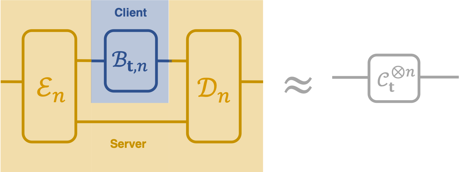
Fig. 2: Remote channel simulation. A client, equipped with a small quantum computer, executes a channel ℬ𝐭,n\mathscr{B}_{\mathbf{t},n}, which enables a server to reproduce nn uses of a target channel 𝒞𝐭\mathscr{C}_{\mathbf{t}}. The part in gold, i.e. the channels ℰn\mathscr{E}_{n} and 𝒟n\mathscr{D}_{n}, are the encoder and the decoder of used by the server to interact with the client, while the part in blue, i.e. the channel ℬ𝐭,n\mathscr{B}_{\mathbf{t},n}, is the channel performed by the client. The protocol is designed so that the overall transformation at the server’s end approximates the target channel 𝒞𝐭⊗n\mathscr{C}_{\mathbf{t}}^{\otimes n} for every choice of 𝐭\mathbf{t} in a given parameter set 𝒯\mathcal{T}.

The remote channel simulation task is depicted in Figure 2. A client, equipped with a small quantum computer, wants a server to execute nn parallel uses of a quantum channel 𝒞𝐭\mathscr{C}_{\mathbf{t}}, chosen from a parametric family {𝒞𝐭}𝐭∈𝒯\{\mathscr{C}_{\mathbf{t}}\}_{\mathbf{t}\in\mathcal{T}}. To this purpose, the server encodes the input of the desired channel 𝒞𝐭⊗n\mathscr{C}_{\mathbf{t}}^{\otimes n} using a quantum channel ℰn∈𝖢𝗁𝖺𝗇⁡(ℋin⊗n,ℋin,n⊗ℳn)\mathscr{E}_{n}\in{\sf Chan}(\mathcal{H}_{\rm in}^{\otimes n},\mathcal{H}_{{\rm in},n}\otimes\mathcal{M}_{n}), called the encoder. The encoder outputs two systems: a small system with Hilbert space ℋin,n\mathcal{H}_{{\rm in},n}, which is sent to the client through a noiseless quantum communication link, and a larger system with Hilbert space ℳn\mathcal{M}_{n}, which is stored in a quantum memory at the server’s end. Then, the client uses its quantum computer to execute a channel ℬ𝐭,n∈𝖢𝗁𝖺𝗇⁡(ℋin,n,ℋout,n)\mathscr{B}_{\mathbf{t},n}\in{\sf Chan}(\mathcal{H}_{{\rm in},n},\mathcal{H}_{{\rm out},n}), producing a small output system with Hilbert space ℋout,n\mathcal{H}_{{\rm out},n}. After the channel ℬ𝐭,n\mathscr{B}_{\mathbf{t},n} has acted, the client sends the output system to the server. Finally, the server applies a decoder 𝒟n∈𝖢𝗁𝖺𝗇⁡(ℋout,n⊗ℳn,ℋout⊗n)\mathscr{D}_{n}\in{\sf Chan}(\mathcal{H}_{{\rm out},n}\otimes\mathcal{M}_{n},\mathcal{H}_{\rm out}^{\otimes n}). The protocol is designed in such a way that the overall transformation 𝒞~𝐭,n:=𝒟n​(ℬ𝐭,n⊗ℐℳn)​ℰn\widetilde{\mathscr{C}}_{\mathbf{t},n}:=\mathscr{D}_{n}(\mathscr{B}_{\mathbf{t},n}\otimes\mathscr{I}_{\mathcal{M}_{n}})\mathscr{E}_{n} is close to the desired channel 𝒞𝐭⊗n\mathscr{C}_{\mathbf{t}}^{\otimes n}.

A remote channel simulation protocol is described by a quadruple 𝖯𝗇:={din,n,dout,n,ℰn,𝒟n}{\sf P_{n}}:=\{d_{{\rm in},n},d_{{\rm out},n},\mathscr{E}_{n},\mathscr{D}_{n}\}. As an error measure, we will use the diamond norm ‖𝒞~𝐭,n−𝒞𝐭⊗n‖⋄\|\widetilde{\mathscr{C}}_{\mathbf{t},n}-\mathscr{C}_{\mathbf{t}}^{\otimes n}\|_{\diamond}. For a remote channel simulation protocol 𝖯n{\sf P}_{n}, we define the simulation error as

ϵsim​(𝖯n):=sup𝐭∈𝒯‖𝒞~𝐭,n−𝒞𝐭⊗n‖⋄.\displaystyle\epsilon_{{\rm sim}}({\sf P}_{n}):=\sup_{\mathbf{t}\in\mathcal{T}}\|\widetilde{\mathscr{C}}_{\mathbf{t},n}-\mathscr{C}_{\mathbf{t}}^{\otimes n}\|_{\diamond}\,. (8)

For a sequence of remote channel simulation protocols {𝖯n}n∈ℕ\{{\sf P}_{n}\}_{n\in\mathbb{N}}, we define the simulation error as ϵsim​({𝖯n}):=lim supn→∞ϵsim​(𝖯n)\epsilon_{\rm sim}(\{{\sf P}_{n}\}):=\limsup_{n\to\infty}\epsilon_{{\rm sim}}({\sf P}_{n}). If the error satisfies the condition ϵsim​({𝖯n})≤ϵsim\epsilon_{\rm sim}(\{{\sf P}_{n}\})\leq\epsilon_{\rm sim} for some non-negative number ϵsim\epsilon_{\rm sim}, then we say that the sequence {𝖯n}\{{\sf P}_{n}\} has error threshold ϵsim\epsilon_{\rm sim}. If ϵsim\epsilon_{\rm sim} is zero, we say that the sequence of protocols {𝖯𝗇}\{{\sf P_{n}}\} has asymptotically vanishing error.

To quantify the communication cost of remote channel simulation, we will use the total number of qubits exchanged between the client and the server, namely Qtot​(n):=log⁡din,n+log⁡dout,nQ_{\rm tot}(n):=\log d_{{\rm in},n}+\log d_{{\rm out},n}, where din,nd_{{\rm in},n} and dout,nd_{{\rm out},n} are the dimensions of the input and output systems of channel ℬ𝐭,n\mathscr{B}_{\mathbf{t},n}. For a sequence of remote channel simulation protocols {𝖯n}n∈ℕ\{{\sf P}_{n}\}_{n\in\mathbb{N}} we will define the regularized simulation cost

σ⁡({𝖯𝗇}):=lim supn→∞Qtot​(n)log⁡n.\displaystyle\sigma(\{{\sf P_{n}}\}):=\limsup_{n\to\infty}\frac{Q_{\rm tot}(n)}{\log n}\,. (9)

The reason for dividing by log⁡n\log n will become clear later in the paper, where we will show that the total number of qubits Qtot​(n)Q_{\rm tot}(n) grows as log⁡n\log n at the leading order.

The infimum of σ⁡({𝖯𝗇})\sigma(\{{\sf P_{n}}\}) over all possible sequences of remote channel simulation protocols with error threshold ϵsim\epsilon_{\rm sim} will be called the regularized simulation cost with error threshold ϵsim\epsilon_{\rm sim}.

The insertion of a quantum channel between an encoder and a decoder, using a quantum memory as in Figure 2, represents the most general transformation from quantum channels to quantum channels. Such transformations are known as a quantum supermap [41, 42, 43]. In our setting, the supermap implemented by the client and server represents the “transmission of a quantum channel” from the client to the server. We stress that the quantum channel 𝒞𝐭⊗n\mathscr{C}_{\mathbf{t}}^{\otimes n} implemented in the protocol is not a communication channel between the client and the server: here, the term “quantum channel” is used as a technical term for a generic quantum process.

We also stress that channel simulation task considered in this paper is different from the task considered in the quantum reverse Shannon theorem [44, 45, 46, 47, 48], which sometimes is also referred to as “channel simulation”. The quantum reverse Shannon theorem concerns the entanglement-assisted classical communication cost of converting an identity channel into a desired channel, in a scenario where the input of the channel is held by one party, and the output of the channel is held by the other party. In contrast, our channel simulation problem concerns the total (classical and quantum) communication cost in a scenario where the input and output of the simulating channel are held by one party, while the input and output of the simulated channel are held by the other party.

The channel communication task described in Section III is a special case of the channel simulation where the input of the channel ℬ𝐭,n\mathscr{B}_{\mathbf{t},n} is trivial, and therefore the channel ℬ𝐭,n\mathscr{B}_{\mathbf{t},n} is simply the preparation of a state η𝐭,n\eta_{\mathbf{t},n}. Hence, every lower bound on the total amount of communication required in the channel simulation scenario is also a lower bound on the amount of communication required in the channel communication scenario.

V Basic notions from quantum metrology

Quantum metrology [29, 30, 31, 32, 31, 33, 34, 35, 36, 37] investigates the use of quantum resources, such as entanglement and coherence, to enhance the precision of parameter estimation.

Refer to caption
Fig. 3: Quantum metrology scheme. A typical scenario in quantum metrology concerns estimation of the channel 𝒞𝐭\mathscr{C}_{\mathbf{t}}, parametrised by unknown parameters 𝐭\mathbf{t}, from nn parallel uses. An experimenter prepares a probe state ψn\psi_{n} and sends part of it through 𝒞𝐭⊗n\mathscr{C}_{\mathbf{t}}^{\otimes n}, keeping the remaining part in a memory. The experimenter then measures jointly the output of 𝒞𝐭⊗n\mathscr{C}_{\mathbf{t}}^{\otimes n} and the state of the memory with a quantum measurement, which, combined with classical data-processing, yields an estimate 𝐭^\hat{\mathbf{t}} of 𝐭\mathbf{t}. The measurement and the classical data-processing are jointly described by a POVM Mn​(d⁡𝐭^)M_{n}(\operatorname{d}\hat{\mathbf{t}}).

In the typical setting, an experimenter is given access to nn parallel uses of a channel 𝒞𝐭\mathscr{C}_{\mathbf{t}} that depends on some unknown parameters 𝐭∈𝒯⊂ℝv\mathbf{t}\in\mathcal{T}\subset\mathbb{R}^{v}. The experimenter then probes the channel in order to obtain an estimate 𝐭^\hat{\mathbf{t}} of the parameters 𝐭\mathbf{t}. The estimation setup consists of the following recipe, illustrated in Figure 3:

  1. 1.

    Prepare a state ψn∈St⁡(ℋin⊗n⊗ℛn)\psi_{n}\in\operatorname{St}\left(\mathcal{H}_{\rm in}^{\otimes n}\otimes\mathcal{R}_{~n}\right), where ℋin\mathcal{H}_{\rm in} is the input Hilbert space of 𝒞𝐭\mathscr{C}_{\mathbf{t}} and ℛn{\mathcal{R}}_{~n} is the Hilbert space of a reference system, unaffected by the action of the channel.

  2. 2.

    Send the nn input systems through 𝒞𝐭⊗n\mathscr{C}_{\mathbf{t}}^{\otimes n}.

  3. 3.

    Measure the nn output systems together with the reference.

  4. 4.

    Use the measurement outcome to produce an estimate 𝐭^\hat{\mathbf{t}}.

The last two steps can be concisely represented by using a positive operator-valued measure (POVM) Mn​(d⁡𝐭^)M_{n}(\operatorname{d}\hat{\mathbf{t}}), which incorporates both the experimental setup used to measure the system and the classical algorithm that produces the estimate 𝐭^\hat{\mathbf{t}} from the measurement outcome.

The error of the estimation procedure can be quantified in terms of the mean squared error (MSE) matrix, defined as

Vi​j​(ψn,𝒞𝐭⊗n,Mn​(d⁡𝐭^))\displaystyle V_{ij}\big(\psi_{n},\mathscr{C}^{\otimes n}_{\mathbf{t}},M_{n}(\operatorname{d}\hat{\mathbf{t}})\big)
:⁣=\displaystyle:= ∫(ti−t^i)​(tj−t^j)​Tr⁡[Mn​(d⁡𝐭^)​𝒞𝐭⊗n​(ψn)].\displaystyle\int\,(t_{i}-\hat{t}_{i})(t_{j}-\hat{t}_{j})\,\operatorname{Tr}\left[M_{n}(\operatorname{d}\hat{\mathbf{t}})\,\mathscr{C}^{\otimes n}_{\mathbf{t}}(\psi_{n})\right]\,. (10)

In the following, we will refer to the trace of the MSE matrix as to the mean squared error (MSE), denoted as

𝖬𝖲𝖤⁡(ψn,𝒞𝐭⊗n,Mn​(d⁡𝐭^)):=Tr⁡[V⁡(ψn,𝒞𝐭⊗n,Mn​(d⁡𝐭^))]\displaystyle{\sf MSE}\big(\psi_{n},\mathscr{C}^{\otimes n}_{\mathbf{t}},M_{n}(\operatorname{d}\hat{\mathbf{t}})\big):=\operatorname{Tr}\Big[V\big(\psi_{n},\mathscr{C}^{\otimes n}_{\mathbf{t}},M_{n}(\operatorname{d}\hat{\mathbf{t}})\big)\Big] (11)

Note that the MSE depends on the value of the true parameter 𝐭\mathbf{t}, which is unknown to the experimenter. To account for this fact, we consider the worst-case over all possible values of 𝐭\mathbf{t}. Minimizing the worst-case MSE over all choices of ψn\psi_{n} and Mn​(d⁡𝐭^)M_{n}(\operatorname{d}\hat{\mathbf{t}}), we obtain the quantity

𝖬𝖲𝖤⁡({𝒞𝐭⊗n}):=min⁡sup𝐭∈𝒯ψ,Mn​(d⁡𝐭^)⁡𝖬𝖲𝖤⁡(ψn,𝒞𝐭⊗n,Mn​(d⁡𝐭^)),\displaystyle{\sf MSE}(\{\mathscr{C}^{\otimes n}_{\mathbf{t}}\}):=\min_{\psi,\,M_{n}(\operatorname{d}\hat{\mathbf{t}})}\,\sup_{\mathbf{t}\in\mathcal{T}}~{\sf MSE}\big(\psi_{n},\mathscr{C}^{\otimes n}_{\mathbf{t}},M_{n}(\operatorname{d}\hat{\mathbf{t}})\big)\,, (12)

which we call the MSE of the channel family {𝒞𝐭⊗n}𝐭∈𝒯\{\mathscr{C}_{\mathbf{t}}^{\otimes n}\}_{\mathbf{t}\in\mathcal{T}}.

The MSE of the channel family {𝒞𝐭⊗n}\{\mathscr{C}_{\mathbf{t}}^{\otimes n}\} vanishes as a function of nn, at a rate that depends on the family. For many channel families, the MSE scales as 1/n1/n, a scaling known as the standard quantum limit [31]. As an example of families with this scaling, we can list families of constant channels, that is, channels of the form 𝒞𝐭​(ρ)=ρ𝐭\mathscr{C}_{\mathbf{t}}(\rho)=\rho_{\mathbf{t}} for some state ρ𝐭\rho_{\mathbf{t}} independent of ρ\rho. For unitary channels, of the form 𝒞𝐭​(ρ)=U𝐭​ρ​U𝐭†\mathscr{C}_{\mathbf{t}}(\rho)=U_{\mathbf{t}}\rho U_{\mathbf{t}}^{\dagger} for some unitary operator U𝐭U_{\mathbf{t}}, the MSE scales as 1/n21/n^{2} [34, 35, 36, 37, 49]. The (1/n2)(1/n^{2})-scaling is referred to as the Heisenberg limit [31].

We say that the channel family {𝒞𝐭⊗n}𝐭∈𝒯\{\mathscr{C}^{\otimes n}_{\mathbf{t}}\}_{\mathbf{t}\in\mathcal{T}} is Heisenberg limited (respectively, standard quantum limited) if its MSE scales as

𝖬𝖲𝖤⁡({𝒞𝐭⊗n})=Θ⁡(n−2)​(respectively,Θ⁡(n−1)),\displaystyle{\sf MSE}\left(\{\mathscr{C}^{\otimes n}_{\mathbf{t}}\}\right)=\Theta\left(n^{-2}\right)\,\left({\rm respectively,}~\Theta\left(n^{-1}\right)\right)\,, (13)

where the notation g⁡(n)=Θ⁡(f⁡(n))g(n)=\Theta\left(f(n)\right) means that g⁡(n)g(n) and f⁡(n)f(n) have the same asymptotic behavior for large enough nn. More precisely, there exists an integer n0n_{0} and two constants c1c_{1} and c2c_{2} such that c1⋅f⁡(n)≤g⁡(n)≤c2⋅f⁡(n)c_{1}\cdot f(n)\leq g(n)\leq c_{2}\cdot f(n) for every n>n0n>n_{0}.

An important tool for deriving bounds on the precision of quantum metrology is the quantum Fisher information matrix, or more precisely, the quantum Fisher information matrices, for there exist multiple quantum versions of the classical Fisher information matrix. In this paper we will mostly use the quantum Fisher information matrix defined in terms of the right logarithmic derivatives (RLDs). For a C1C^{1}-continuous family of quantum states {ρ𝐭}t∈𝒯\{\rho_{\mathbf{t}}\}_{t\in\mathcal{T}}, the RLDs are the operators {LiR}i=1v\{L^{\rm R}_{i}\}_{i=1}^{v} defined via the equation ∂ρ𝐭/∂ti=ρ𝐭​LiR\partial\rho_{\mathbf{t}}/\partial t_{i}=\rho_{\mathbf{t}}L^{\rm R}_{i}. The RLD quantum Fisher information matrix is then defined as

JR​(ρ𝐭):=[Tr⁡((LiR)†​∂ρ𝐭∂tj)]i​j\displaystyle J^{\rm R}(\rho_{\mathbf{t}}):=\left[\operatorname{Tr}\left(\left(L_{i}^{\rm R}\right)^{\dagger}\frac{\partial\rho_{\mathbf{t}}}{\partial t_{j}}\right)\right]_{ij} (14)

For a C1C^{1}-continuous family of quantum channels {𝒞𝐭}⊆𝖢𝗁𝖺𝗇⁡(ℋin,ℋout)\{\mathscr{C}_{\mathbf{t}}\}\subseteq{\sf Chan}(\mathcal{H}_{\rm in},\mathcal{H}_{\rm out}), we define the maximum RLD Fisher information norm as

J𝒞𝐭R:=maxψ∈St⁡(ℋin⊗ℋin)⁡‖JR​((𝒞𝐭⊗ℐin)​(ψ))‖∞,\displaystyle J^{\rm R}_{\mathscr{C}_{\mathbf{t}}}:=\max_{\psi\in\operatorname{St}(\mathcal{H}_{\rm in}\otimes\mathcal{H}_{\rm in})}\left\|J^{\rm R}\Big((\mathscr{C}_{\mathbf{t}}\otimes\mathscr{I}_{\rm in})\,(\psi)\Big)\right\|_{\infty}\,, (15)

where ‖M‖∞:=sup𝐬∈ℝv,‖𝐬‖=1‖M​𝐬‖\|M\|_{\infty}:=\sup_{\mathbf{s}\in\mathbb{R}^{v},\|\mathbf{s}\|=1}\,\|M\mathbf{s}\| denotes the Schatten ∞\infty-norm of a generic real v×vv\times v matrix MM, M​𝐬∈ℝvM\mathbf{s}\in\mathbb{R}^{v} is the vector with components (M​𝐬)i=∑jMi​j​sj(M\mathbf{s})_{i}=\sum_{j}M_{ij}\,s_{j}, and ‖s‖:=∑i=1vsi2\|s\|:=\sqrt{\sum_{i=1}^{v}s_{i}^{2}} is the Euclidean norm.

When the channels {𝒞𝐭}\{\mathscr{C}_{\mathbf{t}}\} satisfy a suitable condition, the RLD Fisher information norm can be computed through a simple analytical expression. The condition is expressed in terms of the Choi operator C𝐭:=Choi⁡(𝒞𝐭)C_{\mathbf{t}}:=\operatorname{Choi}(\mathscr{C}_{\mathbf{t}}) and reads as follows:

Condition 1.

For every vector 𝐬∈ℝv\mathbf{s}\in\mathbb{R}^{v}, the support of the directional derivative (∂C𝐭+x​𝐬/∂x)x=0\left(\partial C_{\mathbf{t}+x\,\mathbf{s}}/\partial x\right)_{x=0} is contained in the support of C𝐭C_{\mathbf{t}}.

When Condition 1 is satisfied, the RLD Fisher information norm has the following expression:

Proposition 1.

If the channel family {𝒞𝐭}𝐭∈𝒯\{\mathscr{C}_{\mathbf{t}}\}_{\mathbf{t}\in\mathcal{T}} satisfies Condition 1 at point 𝐭\mathbf{t}, then its RLD Fisher information norm at 𝐭\mathbf{t} is given by

J𝒞𝐭R=max𝐬∈ℝv,‖𝐬‖=1⁡‖Trout⁡[(∂C𝐭+x​𝐬∂x)x=0​C𝐭−1​(∂C𝐭+x​𝐬∂x)x=0]‖∞.\displaystyle J^{\rm R}_{\mathscr{C}_{\mathbf{t}}}=\max_{\mathbf{s}\in\mathbb{R}^{v},\,\|\mathbf{s}\|=1}\left\|\operatorname{Tr}_{\rm out}\left[\Big(\frac{\partial C_{\mathbf{t}+x\,\mathbf{s}}}{\partial x}\Big)_{x=0}C_{\mathbf{t}}^{-1}\Big(\frac{\partial C_{\mathbf{t}+x\,\mathbf{s}}}{\partial x}\Big)_{x=0}\right]\right\|_{\infty}\,. (16)

The proof is provided in Appendix A.

We note that every channel family satisfying Condition 1 is necessarily standard quantum limited, as proven in Appendix B. The converse is not true: there exist channel families that are standard quantum limited, and yet violate Condition 1. For example, consider a family consisting of constant channels of the form 𝒞𝐭​(⋅):=Tr⁡[⋅]​ψ𝐭\mathscr{C}_{\mathbf{t}}(\cdot):=\operatorname{Tr}[\cdot]\,\psi_{\mathbf{t}}, where {ψ𝐭}⊆𝖯𝗎𝗋𝖲𝗍⁡(ℋout)\{\psi_{\mathbf{t}}\}\subseteq{\sf PurSt}(\mathcal{H}_{\rm out}) is a family of pure states. In this case, the support of the Choi operator C𝐭C_{\mathbf{t}} is 𝖲𝗉𝖺𝗇⁡{|ψ𝐭⟩}⊗ℋin\mathsf{Span}\{|\psi_{\mathbf{t}}\rangle\}\otimes\mathcal{H}_{\rm in}, while the support of its directional derivative is 𝖲𝗉𝖺𝗇⁡{∂|ψ𝐭+x​𝐬⟩/∂x}⊗ℋin\mathsf{Span}\{\partial|\psi_{{\mathbf{t}}+x\,{\mathbf{s}}}\rangle/\partial x\}\otimes\mathcal{H}_{\rm in}, and the two supports are different for some direction 𝐬\mathbf{s}, except in the trivial case where the pure state ψ𝐭\psi_{\mathbf{t}} is independent of 𝐭\mathbf{t}.

VI Main results

Here we summarize the main results of the paper. The standing assumptions for these results are that the channel family under consideration is C1C^{1}-continuous, and that the parameter manifold 𝒯\mathcal{T} is the Cartesian product of vv intervals, namely 𝒯=𝒯1×⋯×𝒯v\mathcal{T}=\mathcal{T}_{1}\times\cdots\times\mathcal{T}_{v}, with 𝒯i=[t0,i,t1,i]\mathcal{T}_{i}=[t_{0,i},t_{1,i}] for i∈{1,…,v}i\in\{1,\dots,v\}.

The first result is a lower bound on the communication cost of remote channel simulation protocols (cf. Figure 2). The cost of remote channel simulation was determined by Fang et al. [50] in terms of the channel’s maximum output mutual information. Our result establishes a connection between the simulation cost and the precision limits of quantum metrology.

Theorem 1 (Quantum metrology lower bound on remote channel simulation).

If the channels {𝒞𝐭⊗n}𝐭∈𝒯\{\mathscr{C}^{\otimes n}_{\mathbf{t}}\}_{\mathbf{t}\in\mathcal{T}} can be estimated with MSE O⁡(n−β)O(n^{-\beta}), then their regularized simulation cost with error threshold ϵsim\epsilon_{{\rm sim}} is lower bounded by (1−ϵsim)​(v​β/2)(1-\epsilon_{{\rm sim}})\,(v\beta/2), where vv is the dimension of the parameter manifold 𝒯\mathcal{T}. In particular, the regularized simulation cost is lower bounded by v​β/2v\beta/2 for all sequences of channel simulation protocols with asymptotically vanishing error.

Theorem 1 implies that the simulation cost of standard quantum limited (respectively, Heisenberg limited) channels grows at least (1−ϵ′)​v/2​log⁡n(1-\epsilon^{\prime})\,v/2\,\log n (respectively, (1−ϵ′)​v​log⁡n(1-\epsilon^{\prime})v\log n) for every ϵ′>ϵsim\epsilon^{\prime}>\epsilon_{\rm sim}. More generally, any intermediate MSE scaling n−βn^{-\beta} will result in a simulation cost of at least (1−ϵ′)​(v​β/2)​log⁡n(1-\epsilon^{\prime})\,(v\beta/2)\,\log n at the leading order in nn.

Theorem 1 also yields a lower bound on the communication cost of quantum channels. Indeed, a protocol that communicates 𝒞𝐭⊗n\mathscr{C}_{\mathbf{t}}^{\otimes n} from the server to the client can be regarded as a special case of remote simulation protocol, with din,n=1d_{{\rm in},n}=1. This argument leads to the following corollary:

Corollary 1.

If the quantum channels {𝒞𝐭⊗n}𝐭∈𝒯\{\mathscr{C}^{\otimes n}_{\mathbf{t}}\}_{\mathbf{t}\in\mathcal{T}} can be estimated with MSE O⁡(n−β)O(n^{-\beta}), then their regularized communication cost with error threshold ϵprog\epsilon_{\rm prog} is lower bounded by (1−ϵprog)​(v​β/2)(1-\epsilon_{{\rm prog}})\,(v\beta/2). In particular, the regularized communication n cost is lower bounded by v​β/2v\beta/2 for all sequences of channel communication protocols with asymptotically vanishing error.

Corollary 1 can be applied to the problem of programming quantum channels. A set of quantum channels {𝒞𝐭}𝐭∈𝒯\{\mathscr{C}_{\mathbf{t}}\}_{\mathbf{t}\in\mathcal{T}} is called programmable if there exist a set of quantum states {η𝐭}𝐭∈𝒯\{\eta_{\mathbf{t}}\}_{\mathbf{t}\in\mathcal{T}} and a quantum channel 𝒲\mathscr{W} so that 𝒞𝐭​(ρ)=𝒲⁡(ρ⊗η𝐭)\mathscr{C}_{\mathbf{t}}(\rho)=\mathscr{W}(\rho\otimes\eta_{\mathbf{t}}) holds for every 𝐭∈𝒯\mathbf{t}\in\mathcal{T}. It is known that programmable quantum channels are standard quantum limited [51, 52, 53, 54]. Corollary 1 implies that the communication cost of programmable channels is at least (1−ϵ′)​v/2​log⁡n(1-\epsilon^{\prime})v/2\,\log n at the leading order in nn, for every ϵ′>ϵsim\epsilon^{\prime}>\epsilon_{\rm sim}.

Our second main result is an achievability result. We provide an explicit channel communication protocol working for a special class of standard quantum limited channels. The protocol is “classical”, in the sense that it can be implemented using only a classical communication channel between the client and the server. The main idea is that the client and the server choose a suitable discretization of the parameter manifold, and the client communicates to the server the point in the discretization that is closest to the label of the desired channel.

The protocol works for channel families {𝒞𝐭}𝐭∈𝒯\{\mathscr{C}_{\mathbf{t}}\}_{\mathbf{t}\in\mathcal{T}} satisfying the following conditions:

Condition 2.

The supremum of the RLD Fisher information norm over the channel family is non-zero, i. e. sup𝐭∈𝒯J𝒞𝐭R>0\sup_{\mathbf{t}\in\mathcal{T}}J^{\rm R}_{\mathscr{C}_{\mathbf{t}}}>0.

Condition 3.

The support of the Choi operator Choi⁡(𝒞𝐭)\operatorname{Choi}({\mathscr{C}_{\mathbf{t}}}) is independent of 𝐭\mathbf{t}.

Condition 2 is rather weak: it simply states that the channel family {𝒞𝐭}\{\mathscr{C}_{\mathbf{t}}\} has a non-trivial dependence on 𝐭\mathbf{t}. In a sense, Condition 3 is also rather weak, in that it is satisfied by all the channels in the interior of the convex set of quantum channels. Such channels have Choi operators with full rank, and therefore satisfy Condition 3. Hence, any quantum channel is arbitrarily close to a channel satisfying Condition 3. On the other hand, Condition 3 rules out some interesting families of quantum channels, such as the families of unitary channels. It is easy to see that Condition 3 is stronger than Condition 1 in Section V. As a consequence, a channel family {𝒞𝐭⊗n}\{\mathscr{C}^{\otimes n}_{\mathbf{t}}\} satisfying Condition 3 is standard quantum limited, cf. Appendix B. The channels satisfying Condition 3 form a strict subset of the standard quantum limited channels: for example, constant channels of the form 𝒞𝐭​(ρ)=|ψ𝐭⟩​⟨ψ𝐭|\mathscr{C}_{\mathbf{t}}(\rho)=|\psi_{\mathbf{t}}\rangle\langle\psi_{\mathbf{t}}| are standard quantum limited, but the support of their Choi operator depends on 𝐭\mathbf{t}. Still, the set of channel families satisfying Condition 3 is large enough to contain interesting examples. For example, it contains all families of Pauli channels of the form 𝒞𝐭:=p0,𝐭​ℐ+px,𝐭​𝒳+py,𝐭​𝒴+pz,𝐭​𝒵\mathscr{C}_{\mathbf{t}}:=p_{0,\mathbf{t}}\,\mathscr{I}+p_{x,\mathbf{t}}\,\mathscr{X}+p_{y,\mathbf{t}}\,\mathscr{Y}+p_{z,\mathbf{t}}\,\mathscr{Z}, where 𝒳,𝒴,𝒵\mathscr{X},\mathscr{Y},\mathscr{Z} are the unitary channels corresponding to the three Pauli matrices, and p𝐭=(p0,𝐭,px,𝐭,py,𝐭,pz,𝐭)p_{\mathbf{t}}=(p_{0,\mathbf{t}},p_{x,\mathbf{t}},p_{y,\mathbf{t}},p_{z,\mathbf{t}}) is a probability distribution with support independent of 𝐭\mathbf{t}.

The details of the channel communication protocols are as follows:

Protocol 1 Communicating nn uses of channel in a family {𝒞𝐭⊗n}𝐭∈𝒯\{\mathscr{C}^{\otimes n}_{\mathbf{t}}\}_{\mathbf{t}\in\mathcal{T}} satisfying Conditions 2 and 3.
1: (Preparation) The client and the server use a discretization of 𝒯\mathcal{T}, denoted by 𝒯n\mathcal{T}_{n} and defined as
𝒯n:={n−α−12v​JmaxR​𝐳|𝐳∈ℤv}∩𝒯,withJmaxR:=sup𝐭∈𝒯J𝒞𝐭R.\displaystyle\mathcal{T}_{n}:=\Bigg\{\frac{n^{-\alpha-\frac{1}{2}}}{\sqrt{vJ^{\rm R}_{\max}}}\mathbf{z}\Bigg|\mathbf{z}\in\mathbb{Z}^{v}\Bigg\}\cap\mathcal{T}\,,\quad{\rm with}\quad J^{\rm R}_{\max}:=\sup_{\mathbf{t}\in\mathcal{T}}J^{\rm R}_{\mathscr{C}_{\mathbf{t}}}\,. (17)
Note that the discretization 𝒯n\mathcal{T}_{n} is well-defined, thanks to Condition 2.
2: (Encoding.) To communicate the channel 𝒞𝐭⊗n\mathscr{C}_{\mathbf{t}}^{\otimes n}, the client finds an element 𝐭n∈𝒯n\mathbf{t}_{n}\in\mathcal{T}_{n} that satisfies
‖𝐭n−𝐭‖<n−α−12JmaxR\displaystyle\|\mathbf{t}_{n}-\mathbf{t}\|<\frac{n^{-\alpha-\frac{1}{2}}}{\sqrt{J^{\rm R}_{\max}}} (18)
in terms of the Euclidean distance. Note that such 𝐭n\mathbf{t}_{n} always exists thanks to Eq. (17). The client encodes the discretized vector 𝐭n\mathbf{t}_{n} into a pure quantum state η𝐭,n=|𝐭n⟩​⟨𝐭n|\eta_{\mathbf{t},n}=|\mathbf{t}_{n}\rangle\langle\mathbf{t}_{n}|, where {|𝐭n⟩}\{|\mathbf{t}_{n}\rangle\} is an orthonormal basis for the Hilbert space of the program system.
3: (Transmission) The client sends the program system to the server.
4: (Decoding.) The server implements 𝒞𝐭n⊗n\mathscr{C}_{\mathbf{t}_{n}}^{\otimes n} on the input state via the following measure-and-operate decoder
𝒟⁡(A⊗B):=∑𝐭n∈𝒯nTr⁡[|𝐭n⟩​⟨𝐭n|​A]​𝒞𝐭n⊗n​(B),\displaystyle\mathscr{D}(A\otimes B):=\sum_{\mathbf{t}_{n}\in\mathcal{T}_{n}}\operatorname{Tr}[|\mathbf{t}_{n}\rangle\langle\mathbf{t}_{n}|A]\,\mathscr{C}_{\mathbf{t}_{n}}^{\otimes n}(B), (19)
where AA and BB are arbitrary operators on the Hilbert space of the program and the Hilbert space of the input, respectively.

The cost and the error rate of the above protocol are quantified in the following theorem, whose proof is provided in Section VIII.

Theorem 2.

Under Conditions 2 and 3, Protocol 1 has an error O⁡(n−α)O(n^{-\alpha}) and costs (1/2+α)​v​log⁡n(1/2+\alpha)v\log n bits of communication at the leading order in nn, where vv is the dimension of the parameter manifold 𝒯\mathcal{T} and α>0\alpha>0 is an arbitrary positive number.

Theorem 2, combined with Corollary 1 implies the optimality of Protocol 1 for communicating channels satisfying Conditions 2 and 3 in the case of asymptotically vanishing error. Indeed, the infimum of the regularized communication cost over all channel communication protocols with ϵprog=0\epsilon_{\rm prog}=0 is exactly v/2​log⁡nv/2\log n, matching the lower bound in Corollary 1.

VII Proof of Theorem 1

VII-A Preliminaries on the inaccuracy of state estimation

The proof of Theorem 1 is based on the notion of inaccuracy of an estimate of a state family [55]. In the following, we will first review a few basic facts about the inaccuracy in state estimation and then we will provide the proof of Theorem 1.

For the estimation of a family of quantum states {ρ𝐭}𝐭∈𝒯\{\rho_{\mathbf{t}}\}_{\mathbf{t}\in\mathcal{T}}, the estimate 𝐭^\hat{\mathbf{t}} is generated by a POVM {M⁡(d⁡𝐭^)}\{M(\operatorname{d}\hat{\mathbf{t}})\}, and its conditional probability distribution is p⁡(d⁡𝐭^|𝐭)=Tr⁡[M⁡(d⁡𝐭^)​ρ𝐭]p(\operatorname{d}\hat{\mathbf{t}}|\mathbf{t})=\operatorname{Tr}[M(\operatorname{d}\hat{\mathbf{t}})\,\rho_{\mathbf{t}}]. We regard the estimate 𝐭^\hat{\mathbf{t}} as the value of a random variable 𝐓^\widehat{\mathbf{T}}, distributed with probability p⁡(d⁡𝐭^|𝐭)p(\operatorname{d}\hat{\mathbf{t}}|\mathbf{t}). The random variable 𝐓^\widehat{\mathbf{T}} will also be called the estimate of the parameter 𝐭\mathbf{t}.

The inaccuracy of the estimate 𝐓^\widehat{\mathbf{T}} quantifies the radius of the smallest Euclidean ball in which the estimate has confidence p∈(0,1)p\in(0,1). Explicitly, the inaccuracy of the estimate 𝐓^\widehat{\mathbf{T}} at the true value 𝐭\mathbf{t} is defined as [55]

δ(p,𝐭,𝐓^):=inf{δ∈ℝ|𝐏𝐫𝐓^|𝐭[∥𝐓^−𝐭∥≤δ]≥p},\displaystyle\delta(p,\mathbf{t},\widehat{\mathbf{T}}):=\inf\Big\{\delta\in\mathbb{R}~\Big|~{{\mathbf{Pr}_{\widehat{\mathbf{T}}|\mathbf{t}}}}\left[\|\widehat{\mathbf{T}}-\mathbf{t}\|\leq\delta\right]\geq p\Big\}, (20)

where 𝐏𝐫𝐓^|𝐭[∥𝐓^−𝐭∥≤δ]\mathbf{Pr}_{\widehat{\mathbf{T}}|\mathbf{t}}\left[\|\widehat{\mathbf{T}}-\mathbf{t}\|\leq\delta\right] is the conditional probability that the random variable 𝐓^\widehat{\mathbf{T}} takes a value 𝐭^\hat{\mathbf{t}} such that the Euclidean distance ‖𝐭^−𝐭‖\|\hat{\mathbf{t}}-\mathbf{t}\| is no larger than δ\delta.

For an arbitrary estimate, the inaccuracy is related to the MSE by the following inequality

δ⁡(p,𝐭,𝐓^)≤𝖬𝖲𝖤⁡(𝐭,𝐓^)1−p∀p∈(0,1),∀𝐭∈𝒯,\displaystyle\delta(p,\mathbf{t},\widehat{\mathbf{T}})\leq\sqrt{\frac{{\sf MSE}(\mathbf{t},\widehat{\mathbf{T}})}{1-p}}\qquad\forall p\in(0,1)\,,\forall\mathbf{t}\in\mathcal{T}\,, (21)

where 𝖬𝖲𝖤⁡(𝐭,𝐓^):=∑i=1v∫p⁡(d⁡𝐭^|𝐭)​(t^i−ti)2{\sf MSE}({\mathbf{t}},\widehat{\mathbf{T}}):=\sum_{i=1}^{v}\int p(\operatorname{d}\hat{\mathbf{t}}|\mathbf{t})\,(\hat{t}_{i}-t_{i})^{2} is the MSE of the estimate 𝐓^\widehat{\mathbf{T}} at the true value 𝐭\mathbf{t} (see Appendix C for a proof). We remind the readers that 𝐓^\hat{\mathbf{T}} in the above definition is a random variable, which takes value 𝐭^\hat{\mathbf{t}} with probability p⁡(d⁡𝐭^|𝐭)p(\operatorname{d}\hat{\mathbf{t}}|\mathbf{t}).

For another state family {ρ𝐭′}𝐭∈𝒯\{\rho_{\mathbf{t}}^{\prime}\}_{\mathbf{t}\in\mathcal{T}}, we have another conditional distribution p′​(d⁡𝐭^|𝐭):=Tr⁡[M⁡(d⁡𝐭^)​ρ𝐭′]p^{\prime}(\operatorname{d}\hat{\mathbf{t}}|\mathbf{t}):=\operatorname{Tr}[M(\operatorname{d}\hat{\mathbf{t}})\,\rho^{\prime}_{\mathbf{t}}]. In the following, we denote the variable subject to the above conditional distribution by 𝐓^′\widehat{\mathbf{T}}^{\prime}, i.e., 𝐏𝐫𝐓^′|𝐭​(d⁡𝐭^)=p′​(d⁡𝐭^|𝐭)\mathbf{Pr}_{\widehat{\mathbf{T}}^{\prime}|\mathbf{t}}(\operatorname{d}\hat{\mathbf{t}})=p^{\prime}(\operatorname{d}\hat{\mathbf{t}}|\mathbf{t}). Hence, we denote the inaccuracy defined (20) with the conditional distribution 𝐏𝐫𝐓^′|𝐭\mathbf{Pr}_{\widehat{\mathbf{T}}^{\prime}|\mathbf{t}} by δ⁡(p,𝐭,𝐓^′)\delta(p,\mathbf{t},\widehat{\mathbf{T}}^{\prime}). If two quantum states ρ𝐭\rho_{\mathbf{t}} and ρ𝐭′\rho_{\mathbf{t}}^{\prime} satisfy the condition ‖ρ𝐭′−ρ𝐭‖1<ϵ\|\rho_{\mathbf{t}}^{\prime}-\rho_{\mathbf{t}}\|_{1}<\epsilon, then the above inaccuracies δ⁡(p,𝐭,𝐓^)\delta(p,\mathbf{t},\widehat{\mathbf{T}}) and δ⁡(p,𝐭,𝐓^′)\delta(p,\mathbf{t},\widehat{\mathbf{T}}^{\prime}) obey the continuity property [55, Eq. (7.1)]

δ⁡(p−ϵ,𝐭,𝐓^)≤δ⁡(p,𝐭,𝐓^′)≤δ⁡(p+ϵ,𝐭,𝐓^).\displaystyle\delta(p-\epsilon,\mathbf{t},\widehat{\mathbf{T}})\leq\delta(p,\mathbf{t},\widehat{\mathbf{T}}^{\prime})\leq\delta(p+\epsilon,\mathbf{t},\widehat{\mathbf{T}})\,. (22)

The inaccuracy is also related to the mutual information between the estimate 𝐭^\hat{\mathbf{t}} and the true parameter 𝐭\mathbf{t}. To establish the relation, one has to assign a prior probability distribution to the true parameter 𝐭\mathbf{t}. Denoting by 𝐓^\hat{\mathbf{T}} the corresponding random variable, one has the following

Lemma 1.

Let 𝐓\mathbf{T} be a vv-dimensional continuous random variable with domain 𝒯=∏i=1v[t0,i,t1,i]\mathcal{T}=\prod_{i=1}^{v}[t_{0,i},t_{1,i}], and let 𝐓^\widehat{\mathbf{T}} be an estimate subject to a conditional distribution 𝐏𝐫𝐓^|𝐭\mathbf{Pr}_{\widehat{\mathbf{T}}|\mathbf{t}} when 𝐓\mathbf{T} takes value 𝐭\mathbf{t}. We define the worst-case inaccuracy δp:=sup𝐭∈𝒯δ⁡(p,𝐭,𝐓^)\delta_{p}:=\sup_{\mathbf{t}\in\mathcal{T}}\delta(p,\mathbf{t},\widehat{\mathbf{T}}), the volume |𝒯|:=∏i=1v(t1,i−t0,i)|\mathcal{T}|:=\prod_{i=1}^{v}(t_{1,i}-t_{0,i}) of the domain, and the volume Bv,δp:=(π​δp)vΓ⁡(v/2+1)B_{v,\delta_{p}}:=\frac{(\sqrt{\pi}\delta_{p})^{v}}{\Gamma(v/2+1)} of a vv-dimensional Euclidean ball with radius δp\delta_{p}, where Γ⁡(y)\Gamma(y) denotes the Gamma function. When the condition

log⁡(1−pp)≤log⁡(2v​|𝒯|−Bv,δpBv,δp)\displaystyle\log\left(\frac{1-p}{p}\right)\leq\log\left(\frac{2^{v}|\mathcal{T}|-B_{v,\delta_{p}}}{B_{v,\delta_{p}}}\right) (23)

holds, the mutual information between 𝐓^\widehat{\mathbf{T}} and 𝐓\mathbf{T}, denoted by I⁡(𝐓^:𝐓)I(\widehat{\mathbf{T}}:{\mathbf{T}}), satisfies the bound

I⁡(𝐓^:𝐓)\displaystyle I(\widehat{\mathbf{T}}:{\mathbf{T}})
≥\displaystyle\geq H⁡(𝐓)−p​log⁡(Bv,δpp)−(1−p)​log⁡(2v​|𝒯|−Bv,δp1−p),\displaystyle H({\mathbf{T}})-p\log\left(\frac{B_{v,\delta_{p}}}{p}\right)-(1-p)\log\left(\frac{2^{v}|\mathcal{T}|-B_{v,\delta_{p}}}{1-p}\right)\,, (24)

where H⁡(𝐓)H({\mathbf{T}}) denotes the differential entropy of the random variable 𝐓\mathbf{T}. The bound can be further weakened to

I⁡(𝐓^:𝐓)≥\displaystyle I(\widehat{\mathbf{T}}:{\mathbf{T}})\geq H⁡(𝐓)−p​v​log⁡(π​δp)+p​log⁡Γ⁡(v2+1)\displaystyle H(\mathbf{T})-pv\log(\sqrt{\pi}\delta_{p})+p\log\Gamma\left(\frac{v}{2}+1\right)
−(1−p)​log⁡(2v​|𝒯|)−h⁡(p).\displaystyle-(1-p)\log(2^{v}|\mathcal{T}|)-h(p)\,. (25)

The proof is provided in Appendix D.

Refer to caption
Fig. 4: Parameter estimation in the remote channel simulation scenario. The estimation of the channel 𝒞𝐭\mathscr{C}_{\mathbf{t}} from nn parallel uses is (approximately) related to the estimation of the channel ℬ𝐭,n\mathscr{B}_{\mathbf{t},n} acting on lower-dimensional quantum systems. In particular, every protocol for estimating 𝒞𝐭\mathscr{C}_{\mathbf{t}} from nn parallel uses can be used as a protocol for estimating channel ℬ𝐭,n\mathscr{B}_{\mathbf{t},n}, by replacing the channel 𝒞𝐭⊗n\mathscr{C}_{\mathbf{t}}^{\otimes n} with the channel 𝒞~𝐭,n:=𝒟n​(ℬ𝐭,n⊗ℐℳ)​ℰn\widetilde{\mathscr{C}}_{\mathbf{t},n}:=\mathscr{D}_{n}(\mathscr{B}_{\mathbf{t},n}\otimes\mathscr{I}_{\mathcal{M}})\mathscr{E}_{n} resulting from a remote channel simulation protocol. The figure shows the general form of such a protocol, consisting in transforming the channel ℬ𝐭,n\mathscr{B}_{\mathbf{t},n} into (an approximation of) channel 𝒞𝐭⊗n\mathscr{C}_{\mathbf{t}}^{\otimes n}, by using an encoder ℰn\mathscr{E}_{n}, and a decoder 𝒟n\mathscr{D}_{n}. The parameter 𝐭\mathbf{t} is then estimated by preparing an input state ψn\psi_{n} for (the approximation of) channel 𝒞𝐭⊗n\mathscr{C}_{\mathbf{t}}^{\otimes n}, and implementing a POVM Mn​(d⁡𝐭^)M_{n}(\operatorname{d}\hat{\mathbf{t}}) on the output.

VII-B Proof of Theorem 1

For the whole proof, pp will denote an arbitrary number in the open interval (0,1−ϵsim)(0,1-\epsilon_{{\rm sim}}). By assumption, the parametric family {𝒞𝐭⊗n}𝐭∈𝒯\{\mathscr{C}^{\otimes n}_{\mathbf{t}}\}_{\mathbf{t}\in\mathcal{T}} can be estimated with MSE O⁡(n−β)O(n^{-\beta}). This means that, for sufficiently large nn, there exist a reference system ℛn\mathcal{R}_{~n}, an input state ψn∈𝖲𝗍⁡(ℋin⊗n⊗ℛn)\psi_{n}\in{\sf St}(\mathcal{H}_{\rm in}^{\otimes n}\otimes\mathcal{R}_{~n}), and a POVM Mn​(d⁡𝐭^)M_{n}(\operatorname{d}\hat{\mathbf{t}}) such that the MSE satisfies the bound

𝖬𝖲𝖤⁡(ψn,𝒞𝐭⊗n,Mn​(d⁡𝐭^))≤c⋅n−β∀𝐭∈𝒯,\displaystyle{\sf MSE}\big(\psi_{n},\mathscr{C}^{\otimes n}_{\mathbf{t}},M_{n}(\operatorname{d}\hat{\mathbf{t}})\big)\leq c\cdot n^{-\beta}\qquad\forall\mathbf{t}\in\mathcal{T}\,, (26)

where c>0c>0 is a suitable constant, and 𝖬𝖲𝖤⁡(ψn,𝒞𝐭⊗n,Mn​(d⁡𝐭^)){\sf MSE}\big(\psi_{n},\mathscr{C}^{\otimes n}_{\mathbf{t}},M_{n}(\operatorname{d}\hat{\mathbf{t}})\big) is the mean squared error defined in Eq. (12).

In this protocol, the output states ρ𝐭,n:=(𝒞𝐭⊗n⊗ℐℛn)​(ψn)\rho_{{\mathbf{t}},n}:=(\mathscr{C}_{\mathbf{t}}^{\otimes n}\otimes\mathscr{I}_{{\mathscr{R}}_{n}})(\psi_{n}) are measured with the POVM Mn​(d⁡𝐭^)M_{n}(\operatorname{d}\hat{\mathbf{t}}). Let 𝐓^n\widehat{\mathbf{T}}_{n} be the estimate with the conditional probability distribution pn​(d⁡𝐭^|𝐭):=Tr⁡[Mn​(d⁡𝐭^)​ρ𝐭,n]p_{n}(\operatorname{d}\hat{\mathbf{t}}|\mathbf{t}):=\operatorname{Tr}[M_{n}(\operatorname{d}\hat{\mathbf{t}})\,\rho_{{\mathbf{t}},n}], and let δ⁡(p,𝐭,𝐓^n)\delta(p,\mathbf{t},\widehat{\mathbf{T}}_{n}) be the corresponding inaccuracy defined in Eq. (20). By inserting Eq. (26) into the bound (21), we obtain the bound

δ⁡(p,𝐭,𝐓^n)≤c(1−p)​nβ∀𝐭∈𝒯.\displaystyle\delta(p,\mathbf{t},\widehat{\mathbf{T}}_{n})\leq\sqrt{\frac{c}{(1-p)n^{\beta}}}\qquad\forall\mathbf{t}\in\mathcal{T}. (27)

Now, let {𝖯n}n∈ℕ\{{\sf P}_{n}\}_{n\in\mathbb{N}} be an arbitrary sequence of remote simulation protocols with error threshold ϵsim\epsilon_{\rm sim}. For each protocol 𝖯n=(din,n,dout,n,ℰn,𝒟n){\sf P}_{n}=(d_{{\rm in},n},d_{{\rm out},n},\mathscr{E}_{n},\mathscr{D}_{n}), consider the channel simulation 𝒞~𝐭,n:=𝒟n​(ℬ𝐭,n⊗ℐℳn)​ℰn\widetilde{\mathscr{C}}_{\mathbf{t},n}:=\mathscr{D}_{n}(\mathscr{B}_{\mathbf{t},n}\otimes\mathscr{I}_{\mathcal{M}_{n}})\mathscr{E}_{n}, and let ϵsim,n:=ϵsim​(𝖯n)\epsilon_{{\rm sim},n}:=\epsilon_{\rm sim}({\sf P}_{n}) be the error defined in Eq. (8). Since the error threshold satisfies the condition ϵsim≥ϵ⁡({𝖯n}):=lim supn→∞ϵsim,n\epsilon_{\rm sim}\geq\epsilon(\{{\sf P}_{n}\}):=\limsup_{n\to\infty}\epsilon_{{\rm sim},n}, and since pp satisfies the condition p<1−ϵsimp<1-\epsilon_{\rm sim}, there exists an integer n0n_{0} such that the condition p<1−ϵsim,np<1-\epsilon_{{\rm sim},n} holds for every n≥n0n\geq n_{0}.

By construction, the output states ρ𝐭,n\rho_{{\mathbf{t}},n} and ρ𝐭,n′:=(𝒞~𝐭,n⊗ℐℛ)​(ψ)\rho_{{\mathbf{t}},n}^{\prime}:=(\widetilde{\mathscr{C}}_{{\mathbf{t}},n}\otimes\mathscr{I}_{\mathscr{R}})(\psi) are at most ϵsim,n\epsilon_{{\rm sim},n} apart from each other in trace norm. Let us denote by 𝐓^n′\widehat{\mathbf{T}}_{n}^{\prime} the variable with the conditional probability distribution 𝐏𝐫𝐓^n′|𝐭​(d​𝐭^)\mathbf{Pr}_{\widehat{\mathbf{T}}_{n}^{\prime}|\mathbf{t}}(d\hat{\mathbf{t}}) given by pn′​(d⁡𝐭^|𝐭):=Tr⁡[Mn​(d⁡𝐭^)​ρ𝐭,n′]p_{n}^{\prime}(\operatorname{d}\hat{\mathbf{t}}|\mathbf{t}):=\operatorname{Tr}[M_{n}(\operatorname{d}\hat{\mathbf{t}})\,\rho_{{\mathbf{t}},n}^{\prime}], and by δ⁡(p,𝐭,𝐓^n′)\delta(p,\mathbf{t},\widehat{\mathbf{T}}_{n}^{\prime}) the corresponding inaccuracy defined in (20). The continuity of the inaccuracy (22) yields the bound

δ⁡(p,𝐭,𝐓^n′)≤δ⁡(p+ϵsim,n,𝐭,𝐓^n)≤c(1−p−ϵsim,n)​nβ\displaystyle\delta(p,\mathbf{t},\widehat{\mathbf{T}}_{n}^{\prime})\leq\delta(p+\epsilon_{{\rm sim},n},\mathbf{t},\widehat{\mathbf{T}}_{n})\leq\sqrt{\frac{c}{(1-p-\epsilon_{{\rm sim},n})n^{\beta}}} (28)

valid for every 𝐭∈𝒯\mathbf{t}\in\mathcal{T} and n≥n0n\geq n_{0}. Since the bound holds for every 𝐭∈𝒯\mathbf{t}\in\mathcal{T}, it also holds for the worst-case inaccuracy δp,n:=max𝐭∈𝒯⁡δ⁡(p,𝐭,𝐓^n′)\delta_{p,n}:=\max_{\mathbf{t}\in\mathcal{T}}\delta(p,\mathbf{t},\widehat{\mathbf{T}}_{n}^{\prime}), which satisfies the inequality

δp,n′≤c(1−p−ϵsim,n)​nβ.\displaystyle\delta_{p,n}^{\prime}\leq\sqrt{\frac{c}{(1-p-\epsilon_{{\rm sim},n})n^{\beta}}}\,. (29)

We now use the relation between the inaccuracy and the mutual information (Lemma 1). Referring to Figure 4 for the labelling of the Hilbert spaces, we have that the total number of transmitted qubits satisfies the bound

Qtot​(n)\displaystyle Q_{\rm tot}(n) :=log⁡d4+log⁡d6≥H⁡(4)+H⁡(6)\displaystyle:=\log d_{4}+\log d_{6}\geq H(4)+H(6)
=H⁡(3,5)+H⁡(6)≥H⁡(3,5,6)\displaystyle=H(3,5)+H(6)\geq H(3,5,6)
≥I(1:3,5,6)≥I(1:8)≡I(𝐓^n′:𝐓),\displaystyle\geq I(1:3,5,6)\geq I(1:8)\equiv I(\widehat{\mathbf{T}}_{n}^{\prime}:\mathbf{T})\,, (30)

where dkd_{k} is the dimension of the Hilbert space of system kk, H⁡(k)H(k) is the von Neumann entropy of the reduced state of system k∈{1,…,8}k\in\{1,\dots,8\}, H⁡(3,5)H(3,5) (respectively, H⁡(3,5,6)H(3,5,6)) is the von Neumann entropy of the composite system made of systems 33 and 55 (respectively, 33, 55, and 66), I(1:3,5,6)I(1:3,5,6) is the mutual information between system 11 and the composite system made of systems 33, 55, and 66, and I⁡(1,8)I(1;8) is the mutual information between systems 11 and 88. The first inequality comes from the maximum value of the von Neumann entropy. The first equality holds since the encoder of the client, i.e. ℰA\mathscr{E}_{A}, can be assumed w.l.o.g. to be isometric. Indeed, for any protocol with a non-isometric ℰA\mathscr{E}_{A}, one can construct a protocol in which ℰA\mathscr{E}_{A} is replaced by its Stinespring dilation with its purifying system traced out at the decoder stage. Such a protocol would have the same error and the same communication cost as the original protocol. The second inequality is the subadditivity of the von Neumann entropy. The third inequality holds since the system labeled by 11 is a classical system, and therefore the conditional entropy is non-negative. The fourth inequality is the data processing inequality of the mutual information.

Now, for p>0p>0 and for large enough nn, the condition (23) holds with the conditional distribution 𝐏𝐫𝐓^n′|𝐭\mathbf{Pr}_{\widehat{\mathbf{T}}_{n}^{\prime}|\mathbf{t}}: indeed, for large enough nn, δp,n′\delta_{p,n}^{\prime} is close to zero (due to Eq. (29)), which implies that Bv,δp,n′B_{v,\delta_{p,n}^{\prime}} is sufficiently small compared to 2v​|𝒯|2^{v}|\mathcal{T}|, and therefore the condition 2v​|𝒯|−Bv,δp,n′Bv,δp,n′≥1−pp\frac{2^{v}|\mathcal{T}|-B_{v,\delta_{p,n}^{\prime}}}{B_{v,\delta_{p,n}^{\prime}}}\geq\frac{1-p}{p} holds, thus implying log⁡2v​|𝒯|−Bv,δp,n′Bv,δp′≥log⁡1−pp\log\frac{2^{v}|\mathcal{T}|-B_{v,\delta_{p,n}^{\prime}}}{B_{v,\delta_{p}^{\prime}}}\geq\log\frac{1-p}{p}.

Since condition (23) holds, we can apply Lemma 1 to the conditional distribution 𝐏𝐫𝐓^n′|𝐭\mathbf{Pr}_{\widehat{\mathbf{T}}_{n}^{\prime}|\mathbf{t}}. Using Eq. (25), we then get

I⁡(𝐓^n′:𝐓)≥\displaystyle I(\widehat{\mathbf{T}}_{n}^{\prime}:\mathbf{T})\geq H⁡(𝐓)−p​v​log⁡(π​δp,n′)−(1−p)​log⁡(2v​|𝒯|)\displaystyle H(\mathbf{T})-pv\log\left(\sqrt{\pi}\,\delta_{p,n}^{\prime}\right)-(1-p)\log\big(2^{v}\,|\mathcal{T}|\big)
+p​log⁡Γ⁡(v2+1)−h⁡(p).\displaystyle+p\log\Gamma\left(\frac{v}{2}+1\right)-h(p)\,. (31)

Since the distribution of 𝐭\mathbf{t} is arbitrary, we can choose it to be uniform, and therefore with entropy H⁡(𝐓)=log⁡|𝒯|H(\mathbf{T})=\log|\mathcal{T}|. The above inequality becomes

I⁡(𝐓^n′:𝐓)≥\displaystyle I(\widehat{\mathbf{T}}_{n}^{\prime}:\mathbf{T})\geq −p​v​log⁡(π​δp,n′)−(1−p)​v\displaystyle-pv\log\left(\sqrt{\pi}\,\delta_{p,n}^{\prime}\right)-(1-p)v
+p​log⁡(|𝒯|​Γ​(v2+1))−h⁡(p).\displaystyle+p\log\left(|\mathcal{T}|\Gamma\left(\frac{v}{2}+1\right)\right)-h(p). (32)

Combining Eq. (VII-B) and Eq. (30), one gets that

Qtot​(n)≥\displaystyle Q_{\rm tot}(n)\geq −p​v​log⁡(π​δp,n′)−(1−p)​v\displaystyle-pv\log\left(\sqrt{\pi}\,\delta_{p,n}^{\prime}\right)-(1-p)v
+p​log⁡(|𝒯|​Γ​(v2+1))−h⁡(p).\displaystyle+p\log\left(|\mathcal{T}|\Gamma\left(\frac{v}{2}+1\right)\right)-h(p). (33)

Inserting Eq. (29) into the above bound, we finally obtain

Qtot​(n)≥\displaystyle Q_{\rm tot}(n)\geq −p​v​log⁡π​c/[(1−p−ϵsim,n)​nβ]−(1−p)​v\displaystyle-pv\log\sqrt{\pi\,c/[(1-p-\epsilon_{{\rm sim},n})n^{\beta}]}-(1-p)v
+p​log⁡(|𝒯|​Γ​(v2+1))−h⁡(p)\displaystyle+p\log\left(|\mathcal{T}|\Gamma\left(\frac{v}{2}+1\right)\right)-h(p)
≥\displaystyle\geq −p​v​log⁡π​c/[(1−p−ϵsim,n)​nβ]−(1−p)​v\displaystyle-pv\log\sqrt{\pi\,c/[(1-p-\epsilon_{{\rm sim},n})n^{\beta}]}-(1-p)v
+p​log⁡(|𝒯|​Γ​(v2+1))−h⁡(p)\displaystyle+p\log\left(|\mathcal{T}|\Gamma\left(\frac{v}{2}+1\right)\right)-h(p)
=\displaystyle= p​v​β2​log⁡n−p​v​log⁡π​c/[(1−p−ϵsim,n)]\displaystyle\frac{pv\beta}{2}\,\log n-pv\log\sqrt{\pi\,c/[(1-p-\epsilon_{{\rm sim},n})]}
−(1−p)​v+p​log⁡(|𝒯|​Γ​(v2+1))−h⁡(p).\displaystyle-(1-p)v+p\log\left(|\mathcal{T}|\Gamma\left(\frac{v}{2}+1\right)\right)-h(p)\,. (34)

Dividing both sides by log⁡n\log n and taking the limit superior, we obtain

lim supn→∞Qtot​(n)log⁡n≥p​v​β2.\displaystyle\limsup_{n\to\infty}\frac{Q_{\rm tot}(n)}{\log n}\geq\frac{pv\beta}{2}. (35)

Since pp is an arbitrary real number in (0,1−ϵsim)(0,1-\epsilon_{{\rm sim}}), the statement in Theorem 1 follows by taking the supremum over pp. ∎

The quantity on the left hand side of Eq. (VII-B) is the mutual information between the true value 𝐭\mathbf{t} and its estimate 𝐭^\hat{\mathbf{t}} in the setting of channel estimation, which amounts to the number of digits of 𝐭\mathbf{t} that can be specified in quantum metrology [56]. When the channel is Heisenberg limited, it is immediate from Eq. (VII-B) that this quantity scales as log⁡n\log n, which was called the “information theoretic Heisenberg limit” in [56], which focussed on the case of ideal phase estimation. Our Eq. (VII-B) establishes a general lower bound on the digitization of estimation precision, which extends the result in [56] from ideal phase estimation to the general noisy and multi-parameter metrology.

VIII Proof of Theorem 2

VIII-A Preliminaries on the RLD Fisher information norm and the 22-Rényi divergence

The proof uses a relation between the RLD Fisher information norm and the 22-Rényi divergence [57, 58, 59, 60].

The 22-Rényi divergence for two states ρ\rho and σ\sigma is defined as D2(ρ||σ)=logTr[ρ2σ−1]D_{2}(\rho||\sigma)=\log\operatorname{Tr}[\rho^{2}\sigma^{-1}] for supp⁡(ρ)⊂supp⁡(σ)\operatorname{supp}(\rho)\subset\operatorname{supp}(\sigma) [57, 58]. The 22-Rényi divergence for states can be extended to a 22-Rényi divergence for quantum channels in the straightforward way: for two channels 𝒜\mathscr{A} and ℬ\mathscr{B}, the 22-Rényi divergence is defined by applying them to an input state (possibly including a reference system), and by maximizing the 22-Rényi divergence of the resulting output states. Explicitly, one has

D2(𝒜||ℬ)\displaystyle D_{2}(\mathscr{A}||\mathscr{B})
:⁣=\displaystyle:= supψ∈PurSt⁡(ℋin⊗ℋin)D2((𝒜⊗ℐin)(ψ)∥(ℬ⊗ℐin)(ψ)).\displaystyle\sup_{\psi\in\operatorname{PurSt}(\mathcal{H}_{\rm in}\otimes\mathcal{H}_{\rm in})}\quad D_{2}\Big(\,(\mathscr{A}\otimes\mathscr{I}_{\rm in})\,(\psi)\Big\|\,(\mathscr{B}\otimes\mathscr{I}_{\rm in})\,(\psi)\Big). (36)

The 22-Rényi divergence of quantum channels is an example of generalized divergence for channels, in the sense of [59, Definition II.2]. Properties of the α\alpha-Rényi divergence for α≥0\alpha\geq 0 have been studied in [60].

Locally, the 22-Rényi divergence is related to the RLD Fisher information norm by the following relation:

Lemma 2.

Let {𝒞𝐭}𝐭∈𝒯\{\mathscr{C}_{\mathbf{t}}\}_{\mathbf{t}\in\mathcal{T}} be a parametric family of quantum channels with the property that all the corresponding Choi operators have the same support. Then, the 2-Rényi divergence has the Taylor expansion

D2(𝒞𝐭′||𝒞𝐭)\displaystyle D_{2}\left(\mathscr{C}_{\mathbf{t}^{\prime}}||\mathscr{C}_{\mathbf{t}}\right) ≤‖𝐭′−𝐭‖2​J𝒞𝐭R+O⁡(‖𝐭′−𝐭‖3)\displaystyle\leq\|\mathbf{t}^{\prime}-\mathbf{t}\|^{2}J^{\rm R}_{\mathscr{C}_{\mathbf{t}}}+O\left(\|\mathbf{t}^{\prime}-\mathbf{t}\|^{3}\right) (37)

for every 𝐭∈𝒯\mathbf{t}\in\mathcal{T} and 𝐭′∈𝒯\mathbf{t}^{\prime}\in\mathcal{T}, where J𝒞𝐭RJ^{\rm R}_{\mathscr{C}_{\mathbf{t}}} is the RLD Fisher information norm defined in Eq. (15).

The proof of Lemma 2 is provided in Appendix E.

VIII-B Proof of Theorem 2

It is not hard to see that the Protocol 1 demands (1/2+α)​v​log⁡n(1/2+\alpha)v\log n bits of communication at the leading order of nn. Indeed, the communication cost is the cost of transmitting an element in the set 𝒯n\mathcal{T}_{n} [cf. Eq. (17)], which can be upper bounded as

log|𝒯n|≤log∏i=1v(t1,i−t0,in−α−12/v​JmaxR+1).\displaystyle\log|\mathcal{T}_{n}|\leq\log\prod_{i=1}^{v}\left(\frac{t_{1,i}-t_{0,i}}{n^{-\alpha-\frac{1}{2}}/\sqrt{vJ^{\rm R}_{\max}}}+1\right)\,. (38)

It is clear from the above bound that the communication cost is (1/2+α)​v​log⁡n(1/2+\alpha)v\log n bits at the leading order of nn.

We now show that the error vanishes as n−αn^{-\alpha}. Recall that the error is ϵprog,n:=sup𝐭∈𝒯ϵprog,n​(𝐭)\epsilon_{{\rm prog},n}:=\sup_{\mathbf{t}\in\mathcal{T}}\epsilon_{{\rm prog},n}(\mathbf{t}) with ϵprog,n​(𝐭):=‖𝒞𝐭n⊗n−𝒞𝐭⊗n‖⋄\epsilon_{{\rm prog},n}(\mathbf{t}):=\left\|\mathscr{C}_{\mathbf{t}_{n}}^{\otimes n}-\mathscr{C}_{\mathbf{t}}^{\otimes n}\right\|_{\diamond}. Let ψ𝐭wc∈PurSt⁡(ℋin⊗n⊗ℋin⊗n)\psi^{\rm wc}_{\mathbf{t}}\in\operatorname{PurSt}\left(\mathcal{H}_{\rm in}^{\otimes n}\otimes\mathcal{H}_{\rm in}^{\otimes n}\right) be the input state such that

‖𝒞𝐭n⊗n−𝒞𝐭⊗n‖⋄\displaystyle\left\|\mathscr{C}_{\mathbf{t}_{n}}^{\otimes n}-\mathscr{C}_{\mathbf{t}}^{\otimes n}\right\|_{\diamond}
=\displaystyle= ‖(𝒞𝐭n⊗n⊗ℐin⊗n)​(ψ𝐭wc)−(𝒞𝐭⊗n⊗ℐin⊗n)​(ψ𝐭wc)‖1.\displaystyle\left\|\,(\mathscr{C}_{\mathbf{t}_{n}}^{\otimes n}\otimes\mathscr{I}_{\rm in}^{\otimes n})\,(\psi^{\rm wc}_{\mathbf{t}})-\,(\mathscr{C}_{\mathbf{t}}^{\otimes n}\otimes\mathscr{I}_{\rm in}^{\otimes n})\,(\psi^{\rm wc}_{\mathbf{t}})\right\|_{1}\,. (39)

Applying Pinsker’s inequality [61], one has

ϵprog,n​(𝐭)\displaystyle\epsilon_{{\rm prog},n}(\mathbf{t})
≤\displaystyle\leq 2log⁡eD1((𝒞𝐭n⊗n⊗ℐin⊗n)(ψwc𝐭)∥(𝒞𝐭⊗n⊗ℐin⊗n)(ψwc𝐭)),\displaystyle\sqrt{\frac{2}{\log e}D_{1}\Big((\mathscr{C}_{\mathbf{t}_{n}}^{\otimes n}\otimes\mathscr{I}_{\rm in}^{\otimes n})(\psi^{\rm wc}_{\mathbf{t}})\Big\|(\mathscr{C}_{\mathbf{t}}^{\otimes n}\otimes\mathscr{I}_{\rm in}^{\otimes n})(\psi^{\rm wc}_{\mathbf{t}})\Big)}\,,

where D1(ρ∥σ):=limα→1Dα(ρ∥σ)=Tr[ρ(logρ−logσ)]D_{1}(\rho\|\sigma):=\lim_{\alpha\to 1}D_{\alpha}(\rho\|\sigma)=\operatorname{Tr}[\rho(\log\rho-\log\sigma)] is the quantum relative entropy, and coincides with the α\alpha-Rényi divergence in the limit α→1\alpha\to 1. Using the monotonicity of the α\alpha-Rényi divergence with respect to α\alpha [62], we then obtain the bound

ϵprog,n​(𝐭)\displaystyle\epsilon_{{\rm prog},n}(\mathbf{t})
≤\displaystyle\leq 2log⁡eD2((𝒞𝐭n⊗n⊗ℐin⊗n)(ψwc𝐭)∥(𝒞𝐭⊗n⊗ℐin⊗n)(ψwc𝐭)).\displaystyle\sqrt{\frac{2}{\log e}D_{2}\Big((\mathscr{C}_{\mathbf{t}_{n}}^{\otimes n}\otimes\mathscr{I}_{\rm in}^{\otimes n})(\psi^{\rm wc}_{\mathbf{t}})\Big\|(\mathscr{C}_{\mathbf{t}}^{\otimes n}\otimes\mathscr{I}_{\rm in}^{\otimes n})(\psi^{\rm wc}_{\mathbf{t}})\Big)}\,. (40)

By definition, of the 22-Rényi divergence for channels, one has

D2((𝒞𝐭n⊗n⊗ℐin⊗n)(ψ𝐭wc)∥(𝒞𝐭⊗n⊗ℐin⊗n)(ψ𝐭wc))\displaystyle D_{2}\Big(\,(\mathscr{C}_{\mathbf{t}_{n}}^{\otimes n}\otimes\mathscr{I}_{\rm in}^{\otimes n})\,(\psi^{\rm wc}_{\mathbf{t}})\Big\|\,(\mathscr{C}_{\mathbf{t}}^{\otimes n}\otimes\mathscr{I}_{\rm in}^{\otimes n})\,(\psi^{\rm wc}_{\mathbf{t}})\Big)
≤\displaystyle\leq D2(𝒞𝐭n⊗n∥𝒞𝐭⊗n).\displaystyle D_{2}\Big(\mathscr{C}^{\otimes n}_{\mathbf{t}_{n}}\Big\|\mathscr{C}^{\otimes n}_{\mathbf{t}}\Big). (41)

Now, we use the fact that the 22-Rényi divergence is additive (see [60, Item 3 of Theorem 3] and Corollary 2 in Appendix E), meaning that we have

D2(𝒞𝐭n⊗n||𝒞𝐭⊗n)=nD2(𝒞𝐭n||𝒞𝐭).\displaystyle D_{2}\left(\mathscr{C}^{\otimes n}_{\mathbf{t}_{n}}||\mathscr{C}^{\otimes n}_{\mathbf{t}}\right)=n\,D_{2}\left(\mathscr{C}_{\mathbf{t}_{n}}||\mathscr{C}_{\mathbf{t}}\right). (42)

Inserting Eqs. (41) and (42) into Eq. (40), we obtain

ϵprog,n​(𝐭)≤2​nlog⁡eD2(𝒞𝐭n||𝒞𝐭).\displaystyle\epsilon_{{\rm prog},n}(\mathbf{t})\leq\sqrt{\frac{2n}{\log e}D_{2}\left(\mathscr{C}_{\mathbf{t}_{n}}||\mathscr{C}_{\mathbf{t}}\right)}. (43)

Finally, we express the 2-Renyi divergence in terms of the RLD Fisher information norm, using Lemma 2. Inserting Eq. (37) into Eq. (43), we obtain the bound

ϵprog,n​(𝐭)\displaystyle\epsilon_{{\rm prog},n}(\mathbf{t}) ≤2​nlog⁡e​[‖𝐭n−𝐭‖2​J𝒞𝐭R+O⁡(‖𝐭n−𝐭‖3)]\displaystyle\leq\sqrt{\frac{2n}{\log e}\,\left[\|\mathbf{t}_{n}-\mathbf{t}\|^{2}J^{\rm R}_{\mathscr{C}_{\mathbf{t}}}+O\left(\|\mathbf{t}_{n}-\mathbf{t}\|^{3}\right)\right]}
≤2​nlog⁡e​[n−2​α−1JmaxR​J𝒞𝐭R+O⁡(‖𝐭n−𝐭‖3)]\displaystyle\leq\sqrt{\frac{2n}{\log e}\,\left[\frac{n^{-2\alpha-1}}{J^{\rm R}_{\max}}\,J^{\rm R}_{\mathscr{C}_{\mathbf{t}}}+O\left(\|\mathbf{t}_{n}-\mathbf{t}\|^{3}\right)\right]}
≤2log⁡e​[n−2​α+O⁡(n−3​α−1/2)]\displaystyle\leq\sqrt{\frac{2}{\log e}\left[n^{-2\alpha}+O(n^{-3\alpha-1/2})\right]}
=2log⁡e​n−α+O⁡(n−2​α−1/2),\displaystyle=\sqrt{\frac{2}{\log e}}\,n^{-\alpha}+O\left(n^{-2\alpha-1/2}\right)\,, (44)

where the second inequality follows from Eq. (18). Since the bound holds for every 𝐭\mathbf{t}, we have proven the error vanishes as n−αn^{-\alpha}. ∎

IX Conclusion

We studied the cost of communicating nn parallel uses of an unknown quantum channel, chosen from a given parametric family. In the direct part, we proposed a protocol for sending the classical description of the channel. In the converse part, we derived a lower bound for the more general task of remote channel simulation, where a client, equipped with a small quantum computer, enables a server to execute a desired quantum channel on a large quantum system. The bound on remote channel simulation yields the desired bound for communicating quantum channels as a corollary. The bound is achieved by our concrete protocol for channels satisfying certain conditions. The bound captures the measurement sensitivity of quantum channels from an information-theoretic point of view and is therefore a step towards the unification of quantum metrology and quantum Shannon theory [56, 63, 55]. Potentially, the bound may have applications in various directions of delegate quantum computation [6], where a server is asked to execute a computation on the state held by a remote client. It can also, for example, be used to determine the bandwidth of a quantum sensor network [64] and to hint on how quantum programs can be conceived. These applications will become more desired as quantum devices are assembled into a network in the near future.

An interesting problem for future research is the compression of multiple-use channels, where the goal is to encode nn uses of an unknown quantum channel 𝒞𝐭\mathscr{C}_{\mathbf{t}} into another quantum channel ℬ𝐭,n\mathscr{B}_{\mathbf{t},n} acting on a smaller system. This task is very similar to the simulation task considered in this paper, except that the parameter 𝐭\mathbf{t} is now invisible. The counterpart of this task for states is the task of compressing multicopy states, recently studied both theoretically [65, 66, 67, 68, 55] and experimentally [69]. The task of channel compression is more involved since the input of the channel is not necessary in the many-copy form, and these compression protocols for states cannot be applied directly. Our bound on remote channel simulation (cf. Theorem 1) applies also to compression, since it is harder. However, it remains open whether a concrete protocol achieving the bound exists.

Appendix A Proof of Proposition 1

In the scalar case v=1v=1, Eq. (16) was shown in [70, Theorem 1]. The extension to the multi-parameter case v>1v>1 can be derived as follows. First, note that one has

J𝒞𝐭R\displaystyle J^{\rm R}_{\mathscr{C}_{\mathbf{t}}}
=\displaystyle= maxψ∈PurSt⁡(ℋin⊗ℋin)max𝐬∈ℝv,‖𝐬‖=1∑i,jsi[JR((𝒞𝐭⊗ℐ)(ψ)]i​jsj\displaystyle\max_{\psi\in\operatorname{PurSt}(\mathcal{H}_{\rm in}\otimes\mathcal{H}_{\rm in})}\,\max_{\mathbf{s}\in\mathbb{R}^{v}\,,\|\mathbf{s}\|=1}\sum_{i,j}\,s_{i}\,\left[J^{\rm R}\Big(\,(\mathscr{C}_{\mathbf{t}}\otimes\mathscr{I})(\psi)\right]_{ij}\,s_{j}
=\displaystyle= max𝐬∈ℝv,‖𝐬‖=1maxψ∈PurSt⁡(ℋin⊗ℋin)∑i,jsi[JR((𝒞𝐭⊗ℐ)(ψ)]i​jsj\displaystyle\max_{\mathbf{s}\in\mathbb{R}^{v}\,,\|\mathbf{s}\|=1}\,\max_{\psi\in\operatorname{PurSt}(\mathcal{H}_{\rm in}\otimes\mathcal{H}_{\rm in})}\,\sum_{i,j}\,s_{i}\,\left[J^{\rm R}\Big(\,(\mathscr{C}_{\mathbf{t}}\otimes\mathscr{I})(\psi)\right]_{ij}\,s_{j}
=\displaystyle= max𝐬∈ℝv,‖𝐬‖=1⁡maxψ∈PurSt⁡(ℋin⊗ℋin)​JR​((𝒟𝐬,x⊗ℐ)​(ψ))\displaystyle\max_{\mathbf{s}\in\mathbb{R}^{v}\,,\|\mathbf{s}\|=1}\,\max_{\psi\in\operatorname{PurSt}(\mathcal{H}_{\rm in}\otimes\mathcal{H}_{\rm in})}\,J^{\rm R}\Big(\,(\mathscr{D}_{\mathbf{s}\,,x}\otimes\mathscr{I})(\psi)\Big)
=\displaystyle= max𝐬∈ℝv,‖𝐬‖=1⁡J𝒟𝐬,xR,\displaystyle\max_{\mathbf{s}\in\mathbb{R}^{v}\,,\|\mathbf{s}\|=1}\,J^{\rm R}_{\mathscr{D}_{\mathbf{s}\,,x}}\,, (45)

where JR​((𝒟𝐬,x⊗ℐ)​(ψ))J^{\rm R}\Big(\,(\mathscr{D}_{\mathbf{s}\,,x}\otimes\mathscr{I})(\psi)\Big) is the RLD Fisher information for the one-parameter family {(𝒟𝐬,x⊗ℐ)​(ψ)}x\{(\mathscr{D}_{\mathbf{s}\,,x}\otimes\mathscr{I})(\psi)\}_{x}, with 𝒟𝐬,x:=𝒞𝐭+x​𝐬\mathscr{D}_{\mathbf{s},x}:=\mathscr{C}_{\mathbf{t}+x\,\mathbf{s}}. Then, [70, Theorem 1] guarantees the equality

J𝒟𝐬,xR=‖Trout⁡[(∂C𝐭+x​𝐬∂x)x=0​C𝐭−1​(∂C𝐭+x​𝐬∂x)x=0]‖∞,\displaystyle J^{\rm R}_{\mathscr{D}_{\mathbf{s}\,,x}}=\left\|\operatorname{Tr}_{\rm out}\left[\left(\frac{\partial C_{\mathbf{t}+x\,\mathbf{s}}}{\partial x}\right)_{x=0}\,C_{\mathbf{t}}^{-1}\,\left(\frac{\partial C_{\mathbf{t}+x\,\mathbf{s}}}{\partial x}\right)_{x=0}\right]\right\|_{\infty}\,, (46)

which, inserted in Eq. (45) yields the desired result.

Appendix B Proof that channels satisfying Condition 1 are standard quantum limited

To prove the desired result, we consider the quantity

K⁡({𝒞𝐭}):=lim supn→∞n​𝖬𝖲𝖤​({𝒞𝐭⊗n})\displaystyle K(\{\mathscr{C}_{\mathbf{t}}\}):=\limsup_{n\to\infty}\,n\,{\sf MSE}(\{\mathscr{C}_{\mathbf{t}}^{\otimes n}\})
=\displaystyle= lim supn→∞min⁡sup𝐭∈𝒯ψn,Mn​(d⁡𝐭^)⁡n​𝖬𝖲𝖤​(ψn,𝒞𝐭⊗n,Mn​(d⁡𝐭^)).\displaystyle\limsup_{n\to\infty}\min_{\psi_{n},M_{n}(\operatorname{d}\hat{\mathbf{t}})}\,\sup_{\mathbf{t}\in\mathcal{T}}~n\,{\sf MSE}\left(\psi_{n},\mathscr{C}^{\otimes n}_{\mathbf{t}},M_{n}(\operatorname{d}\hat{\mathbf{t}})\right)\,. (47)

Note that K⁡({𝒞𝐭})K(\{\mathscr{C}_{\mathbf{t}}\}) is a non-zero constant if and only if the channels {𝒞𝐭}\{\mathscr{C}_{\mathbf{t}}\} are standard quantum limited.

We now show that K⁡({𝒞𝐭})K(\{\mathscr{C}_{\mathbf{t}}\}) is strictly positive for channel families satisfying Condition 1.

Lemma 3.

For a channel family {𝒞𝐭}\{\mathscr{C}_{\mathbf{t}}\} satisfying Condition 1, one has the bound

K⁡({𝒞𝐭})≥1J𝒞𝐭R.\displaystyle K(\{\mathscr{C}_{\mathbf{t}}\})\geq\frac{1}{J^{\rm R}_{\mathscr{C}_{\mathbf{t}}}}. (48)

Proof. First of all, note that one has the bound

K⁡({𝒞𝐭})≥Kla​(𝒞𝐭0)∀t0∈𝒯,\displaystyle K(\{\mathscr{C}_{\mathbf{t}}\})\geq K_{\rm la}(\mathscr{C}_{\mathbf{t}_{0}})\qquad\forall t_{0}\in\mathcal{T}\,, (49)

where Kla​(𝒞𝐭0)K_{\rm la}(\mathscr{C}_{\mathbf{t}_{0}}) is the local asymptotic minimax risk [71], defined as

Kla(𝒞𝐭0):=inf{(ψn,Mn​(d⁡𝐭^))}n∈ℕlimϵ→0\displaystyle K_{\rm la}(\mathscr{C}_{\mathbf{t}_{0}}):=\inf_{\{(\psi_{n},M_{n}(\operatorname{d}\hat{\mathbf{t}}))\}_{n\in\mathbb{N}}}~\lim_{\epsilon\to 0}~
lim supn→∞[sup𝐭∈U⁡(𝐭0,ϵ)n​𝖬𝖲𝖤​(ψn,𝒞𝐭⊗n,Mn​(d⁡𝐭^))],\displaystyle\qquad\limsup_{n\to\infty}\Bigg[\sup_{\mathbf{t}\in U(\mathbf{t}_{0},\epsilon)}\,n\,{\sf MSE}\big(\psi_{n},\mathscr{C}^{\otimes n}_{\mathbf{t}},M_{n}(\operatorname{d}\hat{\mathbf{t}})\big)\Bigg], (50)

where {(ψn,Mn​(d⁡𝐭^))}n∈ℕ\big\{\big(\psi_{n},M_{n}(\operatorname{d}\hat{\mathbf{t}})\big)\big\}_{n\in\mathbb{N}} is a sequence of estimation strategies, consisting of a state ψn\psi_{n} and of a POVM Mn​(d⁡𝐭^)M_{n}(\operatorname{d}\hat{\mathbf{t}}), and U⁡(𝐭0,ϵ)U(\mathbf{t}_{0},\epsilon) is the Euclidean ball of radius ϵ\epsilon centred around 𝐭0\mathbf{t}_{0}. The key difference between Kla​(𝒞𝐭0)K_{\rm la}(\mathscr{C}_{\mathbf{t}_{0}}) and K⁡(𝒞𝐭)K(\mathscr{C}_{\mathbf{t}}) is that Kla​(𝒞𝐭0)K_{\rm la}(\mathscr{C}_{\mathbf{t}_{0}}) focuses on the estimation error in a neighbourhood of a fixed 𝐭0\mathbf{t}_{0}, while K⁡(𝒞𝐭)K(\mathscr{C}_{\mathbf{t}}) concerns the worst-case error over every 𝐭∈𝒯\mathbf{t}\in\mathcal{T}.

Let 𝐬∈Rv\mathbf{s}\in R^{v} be an arbitrary unit vector. By definition, one has

Kla​(𝒞𝐭0)\displaystyle K_{\rm la}(\mathscr{C}_{\mathbf{t}_{0}})
≥\displaystyle\geq limϵ→0inf{(ψn,Mn​(d⁡𝐭^))}n∈ℕ\displaystyle\lim_{\epsilon\to 0}\inf_{\{(\psi_{n},M_{n}(\operatorname{d}\hat{\mathbf{t}}))\}_{n\in\mathbb{N}}}
lim supn→∞[sup𝐭∈U⁡(𝐭0,ϵ)n​𝖬𝖲𝖤​(ψn,𝒞𝐭⊗n,Mn​(d⁡𝐭^))]\displaystyle\qquad\limsup_{n\to\infty}\Bigg[\sup_{\mathbf{t}\in U(\mathbf{t}_{0},\epsilon)}\,n\,{\sf MSE}\big(\psi_{n},\mathscr{C}^{\otimes n}_{\mathbf{t}},M_{n}(\operatorname{d}\hat{\mathbf{t}})\big)\Bigg]
≥\displaystyle\geq limϵ→0lim supn→∞min⁡sup𝐭∈U⁡(𝐭0,ϵ)ψn,Mn​(d⁡𝐭^)⁡n​Tr​[V⁡(ψn,𝒞𝐭⊗n,Mn​(d⁡𝐭^))]\displaystyle\lim_{\epsilon\to 0}\,\limsup_{n\to\infty}\min_{\psi_{n},\,M_{n}(\operatorname{d}\hat{\mathbf{t}})}\,\sup_{\mathbf{t}\in U(\mathbf{t}_{0},\epsilon)}\,n\,\operatorname{Tr}\left[V\big(\psi_{n},\mathscr{C}^{\otimes n}_{\mathbf{t}},M_{n}(\operatorname{d}\hat{\mathbf{t}})\big)\right]
≥\displaystyle\geq limϵ→0lim supn→∞\displaystyle\lim_{\epsilon\to 0}\,\limsup_{n\to\infty}
minψn,Mn​(d⁡𝐭^)⁡[sup𝐭∈U⁡(𝐭0,ϵ)n⁡(∑i,jsi​[V⁡(ψn,𝒞𝐭⊗n,Mn​(d⁡𝐭^))]i​j​sj)]\displaystyle\quad\min_{\psi_{n},\,M_{n}(\operatorname{d}\hat{\mathbf{t}})}\Bigg[\sup_{\mathbf{t}\in U(\mathbf{t}_{0},\epsilon)}\,n\,\left(\sum_{i,j}s_{i}\,\Big[V\big(\psi_{n},\mathscr{C}^{\otimes n}_{\mathbf{t}},M_{n}(\operatorname{d}\hat{\mathbf{t}})\big)\Big]_{ij}\,s_{j}\right)\Bigg]
=\displaystyle= Kla​(𝒟𝐬,x)x=0,\displaystyle K_{\rm la}({\mathscr{D}}_{\mathbf{s},x})_{x=0}\,, (51)

where {𝒟𝐬,x}x\{\mathscr{D}_{\mathbf{s},x}\}_{x} is the one-parameter family defined by 𝒟𝐬,x:=𝒞𝐭0+x​𝐬\mathscr{D}_{\mathbf{s},x}:=\mathscr{C}_{\mathbf{t}_{0}+x\,\mathbf{s}}.

Since the family {𝒞𝐭}\{\mathscr{C}_{\mathbf{t}}\} satisfies Condition 1 at tt, the one-parameter family {𝒟𝐬,x}\{\mathscr{D}_{\mathbf{s},x}\} satisfies Condition 1 at x=0x=0. Hence, [70, Proposition 2] guarantees the condition

Kla​(𝒟𝐬,x)x=0=limn→∞nJ𝒟𝐬,x=0⊗nS,\displaystyle K_{\rm la}(\mathscr{D}_{\mathbf{s},x})_{x=0}=\lim_{n\to\infty}\frac{n}{J^{\rm S}_{{\mathscr{D}}^{\otimes n}_{\mathbf{s},x=0}}}\,, (52)

where J𝒟𝐬,x⊗nS{J^{\rm S}_{{\mathscr{D}}^{\otimes n}_{\mathbf{s},x}}} is the quantum version of the Fisher information based on the symmetric logarithmic derivative (SLD). We omit the definition of the SLD quantum Fisher information because it is not directly relevant here. What is relevant, instead, is the fact that the SLD quantum Fisher information is always upper bounded by the RLD quantum Fisher information [29]. Hence, one has the bound

J𝒟𝐬,x⊗nS≤J𝒟𝐬,x⊗nR=n​J𝒟𝐬,xR,\displaystyle J^{\rm S}_{{\mathscr{D}}^{\otimes n}_{\mathbf{s},x}}\leq J^{\rm R}_{{\mathscr{D}}^{\otimes n}_{\mathbf{s},x}}=n\,J^{\rm R}_{{\mathscr{D}}_{\mathbf{s},x}}, (53)

where the equality follows from the additivity of the RLD quantum Fisher information in the one-parameter case [70, Corollary 1].

Combining this inequality with Equations (51) and (52), we obtain the bound

K⁡({𝒞𝐭})≥1J𝒟𝐬,x=0R∀𝐬∈ℝv​s.t.‖𝐬‖=1.\displaystyle K(\{\mathscr{C}_{\mathbf{t}}\})\geq\frac{1}{J^{\rm R}_{{\mathscr{D}}_{\mathbf{s},x=0}}}\qquad\forall\mathbf{s}\in\mathbb{R}^{v}\,{\rm s.t.}\ \|\mathbf{s}\|=1\,. (54)

Since J𝒞𝐭0R=max𝐬⁡J𝒟𝐬,x=0RJ^{\rm R}_{{\mathscr{C}}_{\mathbf{t}_{0}}}=\max_{\mathbf{s}}\,J^{\rm R}_{{\mathscr{D}}_{\mathbf{s},x=0}} (Equation (45)), this concludes the proof. ∎

In passing, we observe that the inequality (48) yields a necessary condition for the Heisenberg limit scaling (and more generally, for faster-than-standard-quantum-limit scalings): in order to have such scaling, the RLD Fisher information norm must be infinite. This condition can be used to identify families of quantum channels beating the standard quantum limit.

Appendix C Proof of Equation (21)

The proof follows the same steps of the proof of Chebyshev’s inequality. By definition, one has

𝖬𝖲𝖤⁡(𝐭,𝐓^)=∫d⁡𝐭^​‖𝐭^−𝐭‖2​p​(𝐭^|𝐭)\displaystyle{\sf MSE}(\mathbf{t},\widehat{\mathbf{T}})=\int\operatorname{d}\hat{\mathbf{t}}\,\|\hat{\mathbf{t}}-\mathbf{t}\|^{2}\,p(\hat{\mathbf{t}}|\mathbf{t})
=\displaystyle= ∫‖𝐭^−𝐭‖>δd⁡𝐭^​‖𝐭^−𝐭‖2​p​(𝐭^|𝐭)+∫‖𝐭^−𝐭‖≤δd⁡𝐭^​‖𝐭^−𝐭‖2​p​(𝐭^|𝐭)\displaystyle\int_{\|\hat{\mathbf{t}}-\mathbf{t}\|>\delta}\operatorname{d}\hat{\mathbf{t}}\,\|\hat{\mathbf{t}}-\mathbf{t}\|^{2}\,p(\hat{\mathbf{t}}|\mathbf{t})+\int_{\|\hat{\mathbf{t}}-\mathbf{t}\|\leq\delta}\operatorname{d}\hat{\mathbf{t}}\,\|\hat{\mathbf{t}}-\mathbf{t}\|^{2}\,p(\hat{\mathbf{t}}|\mathbf{t})
≥\displaystyle\geq δ2​𝐏𝐫​(‖𝐓^−𝐭‖>δ),\displaystyle\delta^{2}\,\mathbf{Pr}\left(\|\widehat{\mathbf{T}}-\mathbf{t}\|>\delta\right)\,, (55)

and therefore

𝐏𝐫⁡(‖𝐓^−𝐭‖>δ)≤𝖬𝖲𝖤⁡(𝐭,𝐓^)δ2.\displaystyle\mathbf{Pr}\left(\|\widehat{\mathbf{T}}-\mathbf{t}\|>\delta\right)\leq\frac{{\sf MSE}(\mathbf{t},\widehat{\mathbf{T}})}{\delta^{2}}\,. (56)

Thanks to this inequality, every choice of δ\delta satisfying the condition

δ>𝖬𝖲𝖤⁡(𝐭,𝐓^)1−p\displaystyle\delta>\sqrt{\frac{{\sf MSE}(\mathbf{t},\widehat{\mathbf{T}})}{1-p}} (57)

will necessarily satisfy the condition 𝐏𝐫[∥𝐓^−𝐭∥>δ]<1−p\mathbf{Pr}\left[\|\widehat{\mathbf{T}}-\mathbf{t}\|>\delta\right]<1-p. Hence, we obtain

δ(p,𝐭,𝐓^)=inf{δ∈ℝ|𝐏𝐫[∥𝐓^−𝐭∥≤δ]≥p}\displaystyle\delta(p,\mathbf{t},\widehat{\mathbf{T}})=\inf\Big\{\delta\in\mathbb{R}~\Big|~\mathbf{Pr}\left[\|\widehat{\mathbf{T}}-\mathbf{t}\|\leq\delta\right]\geq p\Big\}
≤\displaystyle\leq inf{δ∈ℝ|δ>𝖬𝖲𝖤⁡(𝐭,𝐓^)1−p}=𝖬𝖲𝖤⁡(𝐭,𝐓^)1−p.\displaystyle\inf\left\{\delta\in\mathbb{R}~\left|~\delta>\sqrt{\frac{{\sf MSE}(\mathbf{t},\widehat{\mathbf{T}})}{1-p}}\right\}\right.=\sqrt{\frac{{\sf MSE}(\mathbf{t},\widehat{\mathbf{T}})}{1-p}}\,. (58)

Appendix D Proof of Lemma 1

D-A Preparation

The proof of Lemma 1 uses an auxiliary result, provided in the following:

Lemma 4.

For every estimate 𝐓^\widehat{\mathbf{T}} of a given parameter 𝐭∈𝒯\mathbf{t}\in\mathcal{T}, the worst-case inaccuracy δp:=sup𝐭∈𝒯δ⁡(p,𝐭,𝐓^)\delta_{p}:=\sup_{\mathbf{t}\in\mathcal{T}}\delta(p,\mathbf{t},\widehat{\mathbf{T}}) satisfies the condition

𝐏𝐫[∥𝐓^−𝐭∥≤δp]≥p∀t∈𝒯.\displaystyle\mathbf{Pr}\left[\|\widehat{\mathbf{T}}-\mathbf{t}\|\leq\delta_{p}\right]\geq p\qquad\forall t\in\mathcal{T}\,. (59)

Proof. Let Bδ,𝐭:={𝐭^∈𝒯|‖𝐭^−𝐭‖≤δ}B_{\delta,\mathbf{t}}:=\{\hat{\mathbf{t}}\in\mathcal{T}~|~\|\hat{\mathbf{t}}-\mathbf{t}\|\leq\delta\} the Euclidean ball of radius δ\delta centred at 𝐭\mathbf{t}, and let χδ,𝐭\chi_{\delta,\mathbf{t}} the characteristic function of Bδ,𝐭B_{\delta,\mathbf{t}}. By definition of δ⁡(p,𝐭,𝐓^)\delta(p,\mathbf{t},\widehat{\mathbf{T}}), there exists a sequence {δk}k∈ℕ\{\delta_{k}\}_{k\in\mathbb{N}} such that limk→∞δk=δ⁡(p,𝐭,𝐓^)\lim_{k\to\infty}\delta_{k}=\delta(p,\mathbf{t},\widehat{\mathbf{T}}), and

∫p(d𝐭^|𝐭)χδk,𝐭(𝐭^)=𝐏𝐫[∥𝐓^−𝐭∥≤δk]≥p∀k∈ℕ\displaystyle\int p(\operatorname{d}\hat{\mathbf{t}}|\mathbf{t})\,\chi_{\delta_{k},\mathbf{t}}(\hat{\mathbf{t}})\,=\mathbf{Pr}\left[\|\widehat{\mathbf{T}}-\mathbf{t}\|\leq\delta_{k}\right]\geq p\qquad\forall k\in\mathbb{N} (60)

Note that the sequence {δk}k∈ℕ\{\delta_{k}\}_{k\in\mathbb{N}} can be chosen without loss of generality to be monotonically decreasing, that is, satisfying the condition δk+1≤δk\delta_{k+1}\leq\delta_{k} for every k∈ℕk\in\mathbb{N}. Since the sequence {χδk,𝐭}k∈ℕ\{\chi_{\delta_{k},\mathbf{t}}\}_{k\in\mathbb{N}} converges pointwise to χδ⁡(p,𝐭,𝐓^),𝐭\chi_{\delta(p,\mathbf{t},\widehat{\mathbf{T}}),\mathbf{t}}, and is dominated by the integrable function χδ1,𝐭\chi_{\delta_{1},\mathbf{t}}, the dominated convergence theorem implies

limk→∞∫p⁡(d⁡𝐭^|𝐭)​χδk,𝐭​(𝐭^)=\displaystyle\lim_{k\to\infty}\,\int p(\operatorname{d}\hat{\mathbf{t}}|\mathbf{t})\,\chi_{\delta_{k},\mathbf{t}}(\hat{\mathbf{t}})= ∫p⁡(d⁡𝐭^|𝐭)​χδ⁡(p,𝐭,𝐓^)​𝐭​(𝐭^)\displaystyle\int p(\operatorname{d}\hat{\mathbf{t}}|\mathbf{t})\,\chi_{\delta(p,\mathbf{t},\widehat{\mathbf{T}})\mathbf{t}}(\hat{\mathbf{t}})
=\displaystyle= 𝐏𝐫[∥𝐓^−𝐭∥≤δ(p,𝐭,𝐓^)]\displaystyle\mathbf{Pr}\left[\|\widehat{\mathbf{T}}-\mathbf{t}\|\leq\delta(p,\mathbf{t},\widehat{\mathbf{T}})\right] (61)

Combining Eqs. (62) and (61), we obtain

𝐏𝐫[∥𝐓^−𝐭∥≤δ(p,𝐭,𝐓^)]≥p.\displaystyle\mathbf{Pr}\left[\|\widehat{\mathbf{T}}-\mathbf{t}\|\leq\delta(p,\mathbf{t},\widehat{\mathbf{T}})\right]\geq p\,. (62)

Finally, recall that, by definition, one has δp≥δ⁡(p,𝐭,𝐓^)\delta_{p}\geq\delta(p,\mathbf{t},\widehat{\mathbf{T}}) for every 𝐭∈𝒯\mathbf{t}\in\mathcal{T}. Hence, we have

𝐏𝐫[∥𝐓^−𝐭∥≤δp]≥𝐏𝐫[∥𝐓^−𝐭∥≤δ(p,𝐭,𝐓^)]≥p.\displaystyle\mathbf{Pr}\left[\|\widehat{\mathbf{T}}-\mathbf{t}\|\leq\delta_{p}\right]\geq\mathbf{Pr}\left[\|\widehat{\mathbf{T}}-\mathbf{t}\|\leq\delta(p,\mathbf{t},\widehat{\mathbf{T}})\right]\geq p\,. (63)

∎

We are now ready to provide the proof of Lemma 1.

D-B Proof of Lemma 1

Consider an estimate 𝐓^\widehat{\mathbf{T}} for a vv-dimensional random variable 𝐓\mathbf{T}. The mutual information between the two variables satisfies the bound

I⁡(𝐓^:𝐓)\displaystyle I(\widehat{\mathbf{T}}:\mathbf{T}) =H⁡(𝐓)−H⁡(𝐓|𝐓^)=H⁡(𝐓)−H⁡(𝐓−𝐓^|𝐓^)\displaystyle=H(\mathbf{T})-H(\mathbf{T}|\widehat{\mathbf{T}})=H(\mathbf{T})-H(\mathbf{T}-\widehat{\mathbf{T}}|\widehat{\mathbf{T}})
≥H⁡(𝐓)−H⁡(𝐓−𝐓^),\displaystyle\geq H(\mathbf{T})-H(\mathbf{T}-\widehat{\mathbf{T}}), (64)

where H⁡(𝐗)H(\mathbf{X}) and H⁡(𝐗|𝐘)H(\mathbf{X}|\mathbf{Y}) denote the differential entropy and the conditional differential entropy of two generic random variables 𝐗\mathbf{X} and 𝐘\mathbf{Y}, respectively, and the inequality holds because conditioning of classical random variables does not increase the entropy.

An upper bound on the differential entropy H⁡(𝐓−𝐓^)H({\mathbf{T}}-\widehat{\mathbf{T}}) can be obtained by maximizing it over the probability distributions for the random variable 𝐓−𝐓^\mathbf{T}-\widehat{\mathbf{T}}, under the constraint

𝐏𝐫[∥𝐓^−𝐓∥≤δp]≥p.\displaystyle\mathbf{Pr}\left[\|\widehat{\mathbf{T}}-\mathbf{T}\|\leq\delta_{p}\right]\geq p. (65)

Recall that the domain of the random variable 𝐓\mathbf{T} has the form 𝒯=∏i=1v[t0,i,t1,i]\mathcal{T}=\prod_{i=1}^{v}[t_{0,i},t_{1,i}], and so does 𝐓^\hat{\mathbf{T}}. Therefore, the domain of the random variable 𝐓−𝐓^\mathbf{T}-\widehat{\mathbf{T}} is always contained in the set 𝒯′=∏i=1v[t0,i−t1,i,t1,i−t0,i]\mathcal{T}^{\prime}=\prod_{i=1}^{v}[t_{0,i}-t_{1,i},t_{1,i}-t_{0,i}], whose size is |𝒯′|=2v​|𝒯||\mathcal{T}^{\prime}|=2^{v}|\mathcal{T}|.

Now, let us consider maximizing the differential entropy H⁡(𝐗)H(\mathbf{X}) under the constraint

𝐏𝐫[∥𝐗∥≤δp]≥p\displaystyle\mathbf{Pr}\left[\|\mathbf{X}\|\leq\delta_{p}\right]\geq p (66)

over any random variable 𝐗\mathbf{X} on 𝒯′\mathcal{T}^{\prime}. We choose an additional parameter s≥0s\geq 0 as the following way;

𝐏𝐫[∥𝐗∥≤δp]=p+s.\displaystyle\mathbf{Pr}\left[\|\mathbf{X}\|\leq\delta_{p}\right]=p+s. (67)

Since we are potentially considering a broader class of distributions, the maximum of H⁡(𝐗)H(\mathbf{X}) is an upper bound on H⁡(𝐓−𝐓^)H({\mathbf{T}}-\widehat{\mathbf{T}}). Using Lagrange multipliers, one can show that H⁡(𝐗)H(\mathbf{X}) is maximized when 𝐗\mathbf{X} has a piecewise-constant probability density function. Differentiating the Lagrangian ℒ=−∫p(𝐱)logp(𝐱)+λ0(∫p(𝐱)−1)+λ1(∫|𝐱|≤δp(𝐱)−p−s)\mathcal{L}=-\int p(\mathbf{x})\log p(\mathbf{x})+\lambda_{0}(\int p(\mathbf{x})-1)+\lambda_{1}(\int_{|\mathbf{x}|\leq\delta}p(\mathbf{x})-p-s) shows that p⁡(𝐱)=2λ0+λ1−1/ln⁡2p(\mathbf{x})=2^{\lambda_{0}+\lambda_{1}-1/\ln 2} for |𝐱|≤δ|\mathbf{x}|\leq\delta and p⁡(𝐱)=2λ0−1/ln⁡2p(\mathbf{x})=2^{\lambda_{0}-1/\ln 2} for |𝐱|>δ|\mathbf{x}|>\delta. H⁡(𝐗)H(\mathbf{X}) is then maximized by distributions of the piecewise-constant form:

p(𝐱)={p+sBv,δp|𝐱|≤δp1−p−s2v​|𝒯|−Bv,δp|𝐱|>δp,\displaystyle p(\mathbf{x})=\left\{\begin{matrix}\frac{p+s}{B_{v,\delta_{p}}}&\quad&|\mathbf{x}|\leq\delta_{p}\\ \\ \frac{1-p-s}{2^{v}|\mathcal{T}|-B_{v,\delta_{p}}}&&|\mathbf{x}|>\delta_{p},\end{matrix}\right. (68)

where Bv,δp=(π​δp)vΓ⁡(v/2+1)B_{v,\delta_{p}}=\frac{(\sqrt{\pi}\delta_{p})^{v}}{\Gamma(v/2+1)} denotes the volume of a vv-ball with radius δp\delta_{p}. Hence, the condition (67) implies the inequality;

H⁡(𝐗)≤f⁡(s):=\displaystyle H(\mathbf{X})\leq f(s):= (p+s)​log⁡(Bv,δpp+s)\displaystyle(p+s)\log\left(\frac{B_{v,\delta_{p}}}{p+s}\right)
+(1−p−s)​log⁡(2v​|𝒯|−Bv,δp1−p−s).\displaystyle+(1-p-s)\log\left(\frac{2^{v}|\mathcal{T}|-B_{v,\delta_{p}}}{1-p-s}\right)\,. (69)

Since the condition (23) implies log⁡(1−p−sp+s)≤log⁡(1−pp)≤log⁡(2v​|𝒯|−Bv,δpBv,δp)\log\left(\frac{1-p-s}{p+s}\right)\leq\log\left(\frac{1-p}{p}\right)\leq\log\left(\frac{2^{v}|\mathcal{T}|-B_{v,\delta_{p}}}{B_{v,\delta_{p}}}\right), we have

d​f​(s)d​s=log⁡(Bv,δpp+s)−log⁡(2v​|𝒯|−Bv,δp1−p−s)\displaystyle\frac{df(s)}{ds}=\log\left(\frac{B_{v,\delta_{p}}}{p+s}\right)-\log\left(\frac{2^{v}|\mathcal{T}|-B_{v,\delta_{p}}}{1-p-s}\right)
=\displaystyle= log⁡(1−p−sp+s)−log⁡(2v​|𝒯|−Bv,δpBv,δp)≥0.\displaystyle\log\left(\frac{1-p-s}{p+s}\right)-\log\left(\frac{2^{v}|\mathcal{T}|-B_{v,\delta_{p}}}{B_{v,\delta_{p}}}\right)\geq 0. (70)

Thus, the maximum of the RHS is achieved when s=0s=0. Therefore, due to the condition (65), H⁡(𝐓−𝐓^)H(\mathbf{T}-\widehat{\mathbf{T}}) can be bounded as

H⁡(𝐓−𝐓^)≤p​log⁡(Bv,δpp)+(1−p)​log⁡(2v​|𝒯|−Bv,δp1−p).\displaystyle H(\mathbf{T}-\widehat{\mathbf{T}})\leq p\log\left(\frac{B_{v,\delta_{p}}}{p}\right)+(1-p)\log\left(\frac{2^{v}|\mathcal{T}|-B_{v,\delta_{p}}}{1-p}\right)\,. (71)

Combining Eq. (64) and Eq. (71) we get

I⁡(𝐓^:𝐓)≥\displaystyle I(\widehat{\mathbf{T}}:\mathbf{T})\geq H⁡(𝐓)−p​log⁡(Bv,δpp)\displaystyle H(\mathbf{T})-p\log\left(\frac{B_{v,\delta_{p}}}{p}\right)
−(1−p)​log⁡(2v​|𝒯|−Bv,δp1−p),\displaystyle-(1-p)\log\left(\frac{2^{v}|\mathcal{T}|-B_{v,\delta_{p}}}{1-p}\right)\,, (72)

which coincides with Eq. (24) in the main text.

Furthermore, substituting the expression Bv,δp=(π​δp)vΓ⁡(v/2+1)B_{v,\delta_{p}}=\frac{(\sqrt{\pi}\delta_{p})^{v}}{\Gamma(v/2+1)} into Equation (D-B), we get:

I⁡(𝐓^:𝐓)≥\displaystyle I(\hat{\mathbf{T}}:\mathbf{T})\geq −p​v​log⁡(π​δp)+H⁡(𝐓)+p​log⁡Γ⁡(v2+1)\displaystyle-pv\log(\sqrt{\pi}\delta_{p})+H(\mathbf{T})+p\log\Gamma\left(\frac{v}{2}+1\right)
−h⁡(p)−(1−p)​log⁡(2v​|𝒯|−Bv,δp)\displaystyle-h(p)-(1-p)\log(2^{v}|\mathcal{T}|-B_{v,\delta_{p}})
≥\displaystyle\geq −p​v​log⁡(π​δp)+H⁡(𝐓)+p​log⁡Γ⁡(v2+1)\displaystyle-pv\log(\sqrt{\pi}\delta_{p})+H(\mathbf{T})+p\log\Gamma\left(\frac{v}{2}+1\right)
−h⁡(p)−(1−p)​log⁡(2v​|𝒯|),\displaystyle-h(p)-(1-p)\log(2^{v}|\mathcal{T}|)\,, (73)

where h⁡(p)=−p​log⁡p−(1−p)​log⁡(1−p)h(p)=-p\log p-(1-p)\log(1-p) denotes the binary entropy. The second inequality comes from the monotonicity of logarithm.

Appendix E Proof of Lemma 2

E-A 2-Rényi divergence for quantum channels

The proof of Lemma 2 uses a few properties of the 2-Rényi divergence for quantum channels, reviewed in the following.

First, the 2-Rényi divergence of two quantum channels 𝒜\mathscr{A} and ℬ\mathscr{B} has a finite value if and only if the following condition holds:

Condition 4.

The support of Choi⁡(ℬ)\operatorname{Choi}({\mathscr{B}}) contains the support of Choi⁡(𝒜)\operatorname{Choi}({\mathscr{A}}).

When Condition 4 is satisfied, the 2-Rényi divergence has an explicit expression provided by the following lemma:

Lemma 5.

Let 𝒜\mathscr{A} and ℬ\mathscr{B} be two quantum channels satisfying Condition 4, and let A:=Choi⁡(𝒜)A:=\operatorname{Choi}({\mathscr{A}}) and B:=Choi⁡(ℬ)B:=\operatorname{Choi}({\mathscr{B}}) be their Choi operators. Then, one has

D2(𝒜||ℬ)=log‖Trℋout[AB−1A]‖∞,\displaystyle{D_{2}(\mathscr{A}||\mathscr{B})}=\log\left\|\operatorname{Tr}_{\mathcal{H}_{\rm out}}\,\left[AB^{-1}A\right]\right\|_{\infty}, (74)

where ‖X‖∞:=sup|ψ⟩∈ℋ,|ψ⟩≠0‖X⁡|ψ⟩‖/‖|ψ⟩‖\|X\|_{\infty}:=\sup_{|\psi\rangle\in\mathcal{H},|\psi\rangle\not=0}\,\|X|\psi\rangle\|/\||\psi\rangle\| denotes the operator norm of a generic operator X∈L⁡(ℋ)X\in L(\mathcal{H}).

Proof. Lemma 5 is as a special case of [60, Item 2 of Theorem 3] with α=2\alpha=2. For the reader’s convenience, we provide here a self-contained proof using only elementary techniques.

Let |ψ⟩=∑m=1rpm​|αm⟩⊗|βm⟩|\psi\rangle=\sum_{m=1}^{r}\,\sqrt{p_{m}}\,|\alpha_{m}\rangle\otimes|\beta_{m}\rangle be a Schmidt representation of the state |ψ⟩|\psi\rangle in Equation (36). For 𝒞∈{𝒜,ℬ}\mathscr{C}\in\{\mathscr{A},\mathscr{B}\}, one has (𝒞⊗ℐ)​(ψ)=(Iout⊗F)​Choi⁡(𝒞)​(Iout⊗F)†(\mathscr{C}\otimes\mathscr{I})(\psi)=(I_{\rm out}\otimes F)\operatorname{Choi}(\mathscr{C})(I_{\rm out}\otimes F)^{\dagger}, with F:=∑mpm​|βm⟩​⟨α¯m|F:=\sum_{m}\,\sqrt{p_{m}}\,|\beta_{m}\rangle\langle\overline{\alpha}_{m}|. When FF is invertible, the 22-Rényi divergence between the output states is well-defined thanks to Condition 4, and can be written as

D2((𝒜⊗ℐ)(ψ)∥(ℬ⊗ℐ)(ψ))\displaystyle D_{2}\Big(\,(\mathscr{A}\otimes\mathscr{I})\,(\psi)\Big\|\,(\mathscr{B}\otimes\mathscr{I})\,(\psi)\Big)
=\displaystyle= log{Tr[((Iout⊗F)A(Iout⊗F)†)2\displaystyle\log\Bigg\{\operatorname{Tr}\Bigg[\Big((I_{\rm out}\otimes F)A(I_{\rm out}\otimes F)^{\dagger}\Big)^{2}
⋅((Iout⊗F)B(Iout⊗F)†)−1]}\displaystyle\hskip 77.49976pt\cdot\Big((I_{\rm out}\otimes F)B(I_{\rm out}\otimes F)^{\dagger}\Big)^{-1}\Bigg]\Bigg\}
=\displaystyle= log⁡{Tr⁡[A⁡(Iout⊗F†​F)​A​B−1]}\displaystyle\log\left\{\operatorname{Tr}\left[A(I_{\rm out}\otimes F^{\dagger}F)AB^{-1}\right]\right\}
=\displaystyle= log⁡{Tr⁡[(Iout⊗F†​F)​A​B−1​A]}\displaystyle\log\left\{\operatorname{Tr}\left[(I_{\rm out}\otimes F^{\dagger}F)AB^{-1}A\right]\right\}
=\displaystyle= log⁡{Tr⁡[F†​F​Trout​[A​B−1​A]]}.\displaystyle\log\left\{\operatorname{Tr}\left[F^{\dagger}F\,\operatorname{Tr}_{\rm out}[AB^{-1}A]\,\right]\right\}\,. (75)

When FF is not invertible, one can represent FF as a limit of a sequence of invertible operators, and Equation (75) still holds by continuity.

Note that, for a generic pure state |ψ⟩=∑mpm​|αm⟩​|βm⟩|\psi\rangle=\sum_{m}\,\sqrt{p_{m}}\,|\alpha_{m}\rangle|\beta_{m}\rangle, the operator F†​F=∑mpm​|α¯m⟩​⟨α¯m|F^{\dagger}F=\sum_{m}\,p_{m}\,|\overline{\alpha}_{m}\rangle\langle\overline{\alpha}_{m}| is a generic mixed state. Hence, one has

D2(𝒜||ℬ)\displaystyle D_{2}(\mathscr{A}||\mathscr{B})
=\displaystyle= supψ∈PurSt⁡(ℋin⊗ℋin)D2((𝒜⊗ℐ)(ψ)∥(ℬ⊗ℐ)(ψ))\displaystyle\sup_{\psi\in\operatorname{PurSt}(\mathcal{H}_{\rm in}\otimes\mathcal{H}_{\rm in})}\quad D_{2}\Big(\,(\mathscr{A}\otimes\mathscr{I})\,(\psi)\Big\|\,(\mathscr{B}\otimes\mathscr{I})\,(\psi)\Big)
=\displaystyle= supρ∈St⁡(ℋin)log{Tr[ρTrout[AB−1A]}=log‖Trout[AB−1A]‖∞.\displaystyle\sup_{\rho\in\operatorname{St}(\mathcal{H}_{\rm in})}\,\log\left\{\operatorname{Tr}\left[\rho\,\operatorname{Tr}_{\rm out}[AB^{-1}A\,\right]\right\}=\log\left\|\,\operatorname{Tr}_{\rm out}[AB^{-1}A]\,\right\|_{\infty}\,.

∎

Corollary 2.

If channels 𝒜i\mathscr{A}_{i} and ℬi\mathscr{B}_{i} satisfy Condition 4 for i∈{1,2}i\in\{1,2\}, then the 22-Rényi divergence has the additivity property

D2(𝒜1⊗ℬ1||𝒜2⊗ℬ2)=D2(𝒜1||𝒜2)+D2(ℬ1||ℬ2).\displaystyle D_{2}\left(\mathscr{A}_{1}\otimes\mathscr{B}_{1}||\mathscr{A}_{2}\otimes\mathscr{B}_{2}\right)=D_{2}\left(\mathscr{A}_{1}||\mathscr{A}_{2}\right)+D_{2}\left(\mathscr{B}_{1}||\mathscr{B}_{2}\right)\,. (76)

Proof. Immediate from Equation (74). Corollary 2 is a special case of [60, Item 3 of Theorem 3] with α=2\alpha=2. It can also be derived in a similar way as Theorem 2 of [70]. ∎

Lemma 6.

Let 𝒜\mathscr{A} and ℬ\mathscr{B} be two quantum channels satisfying Condition 4, and let A:=Choi⁡(𝒜)A:=\operatorname{Choi}({\mathscr{A}}) and B:=Choi⁡(ℬ)B:=\operatorname{Choi}({\mathscr{B}}) be their Choi operators. Then, one has

Trout⁡[A​B−1​A]≥Iin\displaystyle\operatorname{Tr}_{{\rm out}}\left[AB^{-1}A\right]\geq I_{\rm in} (77)

and

2D2(𝒜||ℬ)−1=‖Trℋout[(A−B)B−1(A−B)]‖∞.\displaystyle 2^{D_{2}(\mathscr{A}||\mathscr{B})}-1=\left\|\operatorname{Tr}_{\mathcal{H}_{\rm out}}\,\left[(A-B)\,B^{-1}(A-B)\right]\,\right\|_{\infty}\,. (78)

Proof. For a generic unit vector |α⟩∈ℋin|\alpha\rangle\in\mathcal{H}_{\rm in}, one has

⟨α|Trout⁡[A​B−1​A]|α⟩=Tr⁡[|α⟩​⟨α|​Trout​[A​B−1​A]]\displaystyle\langle\alpha|\,\operatorname{Tr}_{{\rm out}}\left[AB^{-1}A\right]\,|\alpha\rangle=\operatorname{Tr}\left[|\alpha\rangle\langle\alpha|\,\operatorname{Tr}_{\rm out}\,\left[AB^{-1}A\right]\right]
=\displaystyle= 2D2((𝒜⊗ℐ)(ψ)∥(ℬ⊗ℐ)(ψ))≥1,\displaystyle 2^{D_{2}\Big(\,(\mathscr{A}\otimes\mathscr{I})\,(\psi)\Big\|\,(\mathscr{B}\otimes\mathscr{I})\,(\psi)\Big)}\geq 1\,, (79)

where |ψ⟩:=|α¯⟩​|α⟩|\psi\rangle:=|\overline{\alpha}\rangle|\alpha\rangle and the second equality follows from Equation (75) with F=|α⟩​⟨α|F=|\alpha\rangle\langle\alpha|, while the inequality follows from the fact that the 2-Rényi divergence of quantum states is non-negative. Since the vector |α⟩|\alpha\rangle is generic, Equation (79) proves Equation (77).

To prove Equation (78), consider first the case where Choi⁡(𝒜)\operatorname{Choi}(\mathscr{A}) and Choi⁡(ℬ)\operatorname{Choi}(\mathscr{B}) are invertible. In this case, one has

Trout⁡[(A−B)​B−1​(A−B)]\displaystyle\operatorname{Tr}_{\rm out}\left[(A-B)\,B^{-1}\,(A-B)\right] =Trout⁡[A​B−1​A+B−2​A]\displaystyle=\operatorname{Tr}_{\rm out}\left[AB^{-1}A+B-2A\right]
=Trout⁡[A​B−1​A]−Iin,\displaystyle=\operatorname{Tr}_{\rm out}\left[AB^{-1}A\right]-I_{\rm in}\,, (80)

having used the relation Trout⁡[A]=Trout⁡[B]=Iin\operatorname{Tr}_{\rm out}[A]=\operatorname{Tr}_{\rm out}[B]=I_{\rm in}.

Hence, one has

∥Trℋout[(Choi(𝒜)−Choi(ℬ))Choi−1(ℬ)\displaystyle\Bigg\|\operatorname{Tr}_{\mathcal{H}_{\rm out}}\,\Bigg[\big(\operatorname{Choi}({\mathscr{A}})-\operatorname{Choi}(\mathscr{B})\big)\operatorname{Choi}^{-1}({\mathscr{B}})
⋅(Choi(𝒜)−Choi(ℬ))]∥∞\displaystyle\hskip 86.11084pt\cdot\big(\operatorname{Choi}({\mathscr{A}})-\operatorname{Choi}(\mathscr{B})\big)\Bigg]\,\Bigg\|_{\infty}
=\displaystyle= ‖Trout⁡[A​B−1​A]−Iin‖∞\displaystyle\left\|\operatorname{Tr}_{\rm out}\left[AB^{-1}A\right]-I_{\rm in}\right\|_{\infty}
=\displaystyle= ‖Trout[AB−1A]‖∞−1=2D2(𝒜||ℬ)−1,\displaystyle\left\|\operatorname{Tr}_{\rm out}\left[AB^{-1}A\right]\right\|_{\infty}-1=2^{D_{2}(\mathscr{A}||\mathscr{B})}-1\,, (81)

the second equality following from Equation (77), and the third equation following from Equation (74). ∎

E-B Proof of Lemma 2

Since the support of the Choi operator of the channels {𝒞𝐭}\{\mathscr{C}_{\mathbf{t}}\} is independent of 𝐭\mathbf{t}, we can apply Lemma 6 with 𝒜=𝒞𝐭′\mathscr{A}=\mathscr{C}_{\mathbf{t}^{\prime}} and ℬ=𝒞𝐭\mathscr{B}=\mathscr{C}_{\mathbf{t}}, obtaining

2D2(𝒞𝐭′||𝒞𝐭)−1\displaystyle 2^{D_{2}(\mathscr{C}_{\mathbf{t}^{\prime}}||\mathscr{C}_{\mathbf{t}})}-1 =‖Trout⁡[(C𝐭′−C𝐭)​C𝐭−1​(C𝐭′−C𝐭)]‖∞,\displaystyle=\left\|\operatorname{Tr}_{{\rm out}}[\,(C_{\mathbf{t}^{\prime}}-C_{\mathbf{t}})\,C_{\mathbf{t}}^{-1}\,(C_{\mathbf{t}^{\prime}}-C_{\mathbf{t}})\,]\,\right\|_{\infty}\,,

where C𝐭C_{\mathbf{t}} and C𝐭′C_{\mathbf{t}^{\prime}} are the Choi operators of channels 𝒞𝐭\mathscr{C}_{\mathbf{t}} and 𝒞𝐭′\mathscr{C}_{\mathbf{t}^{\prime}}, respectively.

Defining ϵ:=‖𝐭′−𝐭‖\epsilon:=\|\mathbf{t}^{\prime}-\mathbf{t}\| and 𝐬:=(𝐭′−𝐭)/‖𝐭′−𝐭‖\mathbf{s}:=(\mathbf{t}^{\prime}-\mathbf{t})/\|\mathbf{t}^{\prime}-\mathbf{t}\|, the Taylor expansion of the operator C𝐭′C_{\mathbf{t}^{\prime}}

2D2(𝒞𝐭′||𝒞𝐭)−1\displaystyle 2^{D_{2}(\mathscr{C}_{\mathbf{t}^{\prime}}||\mathscr{C}_{\mathbf{t}})}-1
=\displaystyle= ‖Trℋout⁡(ϵ​∑i∂C𝐭∂ti​si+O⁡(ϵ2))​C𝐭−1​(ϵ​∑j∂C𝐭∂tj​sj+O⁡(ϵ2))‖∞\displaystyle\Big\|\operatorname{Tr}_{\mathcal{H}_{\rm out}}\Big(\epsilon\,\sum_{i}\frac{\partial C_{\mathbf{t}}}{\partial t_{i}}\,s_{i}+O(\epsilon^{2})\Big)C_{\mathbf{t}}^{-1}\,\Big(\epsilon\,\sum_{j}\frac{\partial C_{\mathbf{t}}}{\partial t_{j}}\,s_{j}+O(\epsilon^{2})\Big)\Big\|_{\infty}
=\displaystyle= ϵ2​‖∑i,jsi​sj​Trℋout⁡(∂C𝐭∂ti​C𝐭−1​∂C𝐭∂tj)‖∞+O⁡(ϵ3),\displaystyle\epsilon^{2}\left\|\sum_{i,j}s_{i}s_{j}\operatorname{Tr}_{\mathcal{H}_{\rm out}}\left(\frac{\partial C_{\mathbf{t}}}{\partial t_{i}}C_{\mathbf{t}}^{-1}\,\frac{\partial C_{\mathbf{t}}}{\partial t_{j}}\right)\right\|_{\infty}+O\left(\epsilon^{3}\right)\,, (82)

where the O⁡(ϵ3)O\left(\epsilon^{3}\right) can be uniformly bounded with respect to 𝐬\mathbf{s}.

Substituting Eq. (16) into Eq. (82), one gets

2D2(𝒞𝐭+ϵ​𝐬||𝒞𝐭)−1≤ϵ2J𝒞𝐭R+O(ϵ3),\displaystyle 2^{D_{2}(\mathscr{C}_{\mathbf{t}+\epsilon\mathbf{s}}||\mathscr{C}_{\mathbf{t}})}-1\leq\epsilon^{2}J^{\rm R}_{\mathscr{C}_{\mathbf{t}}}+O\left(\epsilon^{3}\right)\,, (83)

which proves the desired result. ∎

References

  • [1] A. C.-C. Yao, “Some complexity questions related to distributive computing(preliminary report),” in Proceedings of the Eleventh Annual ACM Symposium on Theory of Computing, ser. STOC ’79. New York, NY, USA: ACM, 1979, pp. 209–213. [Online]. Available: http://doi.acm.org/10.1145/800135.804414
  • [2] N. A. Lynch, Distributed algorithms. Elsevier, 1996.
  • [3] W. Dargie and C. Poellabauer, Fundamentals of wireless sensor networks: theory and practice. John Wiley & Sons, 2010.
  • [4] D. Gottesman and I. L. Chuang, “Demonstrating the viability of universal quantum computation using teleportation and single-qubit operations,” Nature, vol. 402, no. 6760, pp. 390–393, 1999.
  • [5] A. Sørensen and K. Mølmer, “Error-free quantum communication through noisy channels,” Physical Review A, vol. 58, pp. 2745–2749, Oct 1998. [Online]. Available: https://link.aps.org/doi/10.1103/PhysRevA.58.2745
  • [6] A. M. Childs, “Secure assisted quantum computation,” Quantum Information & Computation, vol. 5, no. 6, pp. 456–466, 2005.
  • [7] A. Broadbent, J. Fitzsimons, and E. Kashefi, “Universal blind quantum computation,” in 2009 50th Annual IEEE Symposium on Foundations of Computer Science. IEEE, 2009, pp. 517–526.
  • [8] J. F. Fitzsimons and E. Kashefi, “Unconditionally verifiable blind quantum computation,” Physical Review A, vol. 96, no. 1, p. 012303, 2017.
  • [9] E. Kashefi and A. Pappa, “Multiparty delegated quantum computing,” Cryptography, vol. 1, no. 2, p. 12, 2017.
  • [10] M. A. Nielsen and I. L. Chuang, “Programmable quantum gate arrays,” Physical Review Letters, vol. 79, no. 2, p. 321, 1997.
  • [11] J. Fiurášek, M. Dušek, and R. Filip, “Universal measurement apparatus controlled by quantum software,” Physical Review Letters, vol. 89, no. 19, p. 190401, 2002.
  • [12] J. A. Bergou and M. Hillery, “Universal programmable quantum state discriminator that is optimal for unambiguously distinguishing between unknown states,” Physical Review Letters, vol. 94, no. 16, p. 160501, 2005.
  • [13] M. Hillery, M. Ziman, and V. Bužek, “Approximate programmable quantum processors,” Physical Review A, vol. 73, no. 2, p. 022345, 2006.
  • [14] G. M. D’Ariano and P. Perinotti, “Efficient universal programmable quantum measurements,” Physical Review Letters, vol. 94, no. 9, p. 090401, 2005.
  • [15] S. Ishizaka and T. Hiroshima, “Asymptotic teleportation scheme as a universal programmable quantum processor,” Physical Review Letters, vol. 101, no. 24, p. 240501, 2008.
  • [16] M. Sedlák, A. Bisio, and M. Ziman, “Optimal probabilistic storage and retrieval of unitary channels,” Physical Review Letters, vol. 122, no. 17, p. 170502, 2019.
  • [17] A. M. Kubicki, C. Palazuelos, and D. Pérez-García, “Resource quantification for the no-programing theorem,” Physical Review Letters, vol. 122, no. 8, p. 080505, 2019.
  • [18] G. Chiribella, G. M. D’Ariano, and P. Perinotti, “Optimal cloning of unitary transformation,” Physical Review Letters, vol. 101, no. 18, p. 180504, 2008.
  • [19] W. Dür, P. Sekatski, and M. Skotiniotis, “Deterministic superreplication of one-parameter unitary transformations,” Physical Review Letters, vol. 114, no. 12, p. 120503, 2015.
  • [20] G. Chiribella, Y. Yang, and C. Huang, “Universal superreplication of unitary gates,” Physical Review Letters, vol. 114, no. 12, p. 120504, 2015.
  • [21] G. Chiribella and D. Ebler, “Optimal quantum networks and one-shot entropies,” New Journal of Physics, vol. 18, no. 9, p. 093053, 2016.
  • [22] J. Miyazaki, A. Soeda, and M. Murao, “Universal quantum algorithm to complex conjugate unitary gates and implications,” arXiv preprint arXiv:1706.03481, 2017.
  • [23] Y. Yang, G. Chiribella, and Q. Hu, “Units of rotational information,” New Journal of Physics, vol. 19, no. 12, p. 123003, 2017.
  • [24] I. L. Chuang and M. A. Nielsen, “Prescription for experimental determination of the dynamics of a quantum black box,” Journal of Modern Optics, vol. 44, no. 11-12, pp. 2455–2467, 1997.
  • [25] J. Poyatos, J. I. Cirac, and P. Zoller, “Complete characterization of a quantum process: the two-bit quantum gate,” Physical Review Letters, vol. 78, no. 2, p. 390, 1997.
  • [26] J. B. Altepeter, D. Branning, E. Jeffrey, T. Wei, P. G. Kwiat, R. T. Thew, J. L. O’Brien, M. A. Nielsen, and A. G. White, “Ancilla-assisted quantum process tomography,” Physical Review Letters, vol. 90, no. 19, p. 193601, 2003.
  • [27] S. Pirandola, “Quantum reading of a classical digital memory,” Physical Review Letters, vol. 106, no. 9, p. 090504, 2011.
  • [28] S. Pirandola, C. Lupo, V. Giovannetti, S. Mancini, and S. L. Braunstein, “Quantum reading capacity,” New Journal of Physics, vol. 13, no. 11, p. 113012, 2011.
  • [29] A. Holevo, Probabilistic and statistical aspects of quantum theory. North-Holland, 1982.
  • [30] C. W. Helstrom, Quantum detection and estimation theory. Academic press, 1976.
  • [31] V. Giovannetti, S. Lloyd, and L. Maccone, “Quantum metrology,” Physical Review Letters, vol. 96, no. 1, p. 010401, 2006.
  • [32] ——, “Advances in quantum metrology,” Nature photonics, vol. 5, no. 4, p. 222, 2011.
  • [33] A. Luis and J. Peřina, “Optimum phase-shift estimation and the quantum description of the phase difference,” Physical Review A, vol. 54, no. 5, p. 4564, 1996.
  • [34] V. Bužek, R. Derka, and S. Massar, “Optimal quantum clocks,” Physical Review Letters, vol. 82, no. 10, p. 2207, 1999.
  • [35] G. Chiribella, G. M. D’Ariano, P. Perinotti, and M. F. Sacchi, “Efficient use of quantum resources for the transmission of a reference frame,” Physical Review Letters, vol. 93, no. 18, p. 180503, 2004.
  • [36] E. Bagan, M. Baig, and R. Munoz-Tapia, “Quantum reverse engineering and reference-frame alignment without nonlocal correlations,” Physical Review A, vol. 70, no. 3, p. 030301, 2004.
  • [37] M. Hayashi, “Parallel treatment of estimation of su (2) and phase estimation,” Physics Letters A, vol. 354, no. 3, pp. 183–189, 2006.
  • [38] M.-D. Choi, “Completely positive linear maps on complex matrices,” Linear algebra and its applications, vol. 10, no. 3, pp. 285–290, 1975.
  • [39] S. Pirandola, R. Laurenza, C. Ottaviani, and L. Banchi, “Fundamental limits of repeaterless quantum communications,” Nature Communications, vol. 8, p. 15043, 2017.
  • [40] S. Das and M. M. Wilde, “Quantum reading capacity: General definition and bounds,” IEEE Transactions on Information Theory, vol. 65, no. 11, pp. 7566–7583, 2019.
  • [41] G. Chiribella, G. M. D’Ariano, and P. Perinotti, “Transforming quantum operations: Quantum supermaps,” EPL (Europhysics Letters), vol. 83, no. 3, p. 30004, 2008.
  • [42] ——, “Theoretical framework for quantum networks,” Physical Review A, vol. 80, no. 2, p. 022339, 2009.
  • [43] G. Chiribella, G. M. D’Ariano, P. Perinotti, and B. Valiron, “Quantum computations without definite causal structure,” Physical Review A, vol. 88, no. 2, p. 022318, 2013.
  • [44] C. H. Bennett, P. W. Shor, J. A. Smolin, and A. V. Thapliyal, “Entanglement-assisted capacity of a quantum channel and the reverse shannon theorem,” IEEE Transactions on Information Theory, vol. 48, no. 10, pp. 2637–2655, 2002.
  • [45] M. Berta, M. Christandl, and R. Renner, “A conceptually simple proof of the quantum reverse shannon theorem,” in Conference on Quantum Computation, Communication, and Cryptography. Springer, 2010, pp. 131–140.
  • [46] ——, “The quantum reverse shannon theorem based on one-shot information theory,” Communications in Mathematical Physics, vol. 306, no. 3, p. 579, 2011.
  • [47] N. Datta, M.-H. Hsieh, and M. M. Wilde, “Quantum rate distortion, reverse shannon theorems, and source-channel separation,” IEEE Transactions on Information Theory, vol. 59, no. 1, pp. 615–630, 2012.
  • [48] C. H. Bennett, I. Devetak, A. W. Harrow, P. W. Shor, and A. Winter, “The quantum reverse shannon theorem and resource tradeoffs for simulating quantum channels,” IEEE Transactions on Information Theory, vol. 60, no. 5, pp. 2926–2959, 2014.
  • [49] J. Kahn, “Fast rate estimation of a unitary operation in su (d),” Physical Review A, vol. 75, no. 2, p. 022326, 2007.
  • [50] K. Fang, X. Wang, M. Tomamichel, and M. Berta, “Quantum channel simulation and the channel’s smooth max-information,” IEEE Transactions on Information Theory, pp. 1–1, 2019.
  • [51] Z. Ji, G. Wang, R. Duan, Y. Feng, and M. Ying, “Parameter estimation of quantum channels,” IEEE Transactions on Information Theory, vol. 54, no. 11, pp. 5172–5185, 2008.
  • [52] S. Pirandola and C. Lupo, “Ultimate precision of adaptive noise estimation,” Physical Review Letters, vol. 118, no. 10, p. 100502, 2017.
  • [53] ——, “Erratum: Ultimate precision of adaptive noise estimation [phys. rev. lett. 118, 100502 (2017)],” Physical Review Letters, vol. 119, no. 12, p. 129901, 2017.
  • [54] M. Takeoka and M. M. Wilde, “Optimal estimation and discrimination of excess noise in thermal and amplifier channels,” arXiv preprint arXiv:1611.09165, 2016.
  • [55] Y. Yang, G. Chiribella, and M. Hayashi, “Quantum stopwatch: how to store time in a quantum memory,” Proceedings of the Royal Society A, vol. 474, no. 2213, p. 20170773, 2018.
  • [56] M. Hassani, C. Macchiavello, and L. Maccone, “Digital quantum estimation,” Physical Review Letters, vol. 119, no. 20, p. 200502, 2017.
  • [57] N. Sharma and N. A. Warsi, “Fundamental bound on the reliability of quantum information transmission,” Physical Review Letters, vol. 110, no. 8, p. 080501, 2013.
  • [58] M. M. Wilde, A. Winter, and D. Yang, “Strong converse for the classical capacity of entanglement-breaking and hadamard channels via a sandwiched rényi relative entropy,” Communications in Mathematical Physics, vol. 331, no. 2, pp. 593–622, 2014.
  • [59] F. Leditzky, E. Kaur, N. Datta, and M. M. Wilde, “Approaches for approximate additivity of the Holevo information of quantum channels,” Physical Review A, vol. 97, no. 1, p. 012332, 2018.
  • [60] K. Fang and H. Fawzi, “Geometric Rényi divergence and its applications in quantum channel capacities,” arXiv preprint arXiv:1909.05758, 2019.
  • [61] M. Ohya and D. Petz, Quantum entropy and its use. Springer Science & Business Media, 2004.
  • [62] M. Müller-Lennert, F. Dupuis, O. Szehr, S. Fehr, and M. Tomamichel, “On quantum rényi entropies: A new generalization and some properties,” Journal of Mathematical Physics, vol. 54, no. 12, p. 122203, 2013.
  • [63] J. Czajkowski, M. Jarzyna, and R. Demkowicz-Dobrzański, “Super-additivity in communication of classical information through quantum channels from a quantum parameter estimation perspective,” New Journal of Physics, vol. 19, no. 7, p. 073034, 2017.
  • [64] P. Komar, E. M. Kessler, M. Bishof, L. Jiang, A. S. Sørensen, J. Ye, and M. D. Lukin, “A quantum network of clocks,” Nature Physics, vol. 10, no. 8, p. 582, 2014.
  • [65] M. Plesch and V. Bužek, “Efficient compression of quantum information,” Physical Review A, vol. 81, no. 3, p. 032317, 2010.
  • [66] Y. Yang, G. Chiribella, and D. Ebler, “Efficient quantum compression for ensembles of identically prepared mixed states,” Physical Review Letters, vol. 116, no. 8, p. 080501, 2016.
  • [67] Y. Yang, G. Chiribella, and M. Hayashi, “Optimal compression for identically prepared qubit states,” Physical Review Letters, vol. 117, no. 9, p. 090502, 2016.
  • [68] Y. Yang, G. Bai, G. Chiribella, and M. Hayashi, “Compression for quantum population coding,” IEEE Transactions on Information Theory (Early Access), 2018.
  • [69] L. A. Rozema, D. H. Mahler, A. Hayat, P. S. Turner, and A. M. Steinberg, “Quantum data compression of a qubit ensemble,” Physical Review Letters, vol. 113, no. 16, p. 160504, 2014.
  • [70] M. Hayashi, “Comparison between the cramer-rao and the mini-max approaches in quantum channel estimation,” Communications in Mathematical Physics, vol. 304, no. 3, pp. 689–709, 2011.
  • [71] J. Hájek, “Local asymptotic minimax and admissibility in estimation,” in Proceedings of the sixth Berkeley symposium on mathematical statistics and probability, vol. 1, 1972, pp. 175–194.